Spatial Analysis of Regional Income Inequality

SERGIO J. REY

Department of GeographySan Diego State University

and

Regional Economics Applications Laboratory

University of Illinois

October 15, 2001

Abstract

Questions surrounding regional economic convergence have commanded a greatdeal of recent attention in economics literature. As in other recent cases in the so-cial sciences, the application of spatially explicit methods of data analysis to theconvergence question has yielded important insights on regional economic growth.

By contrast, the literature on regional income inequality, although somewhatolder than the convergence literature, has been slower to adopt new spatially ex-plicit methods of data analysis. This chapter helps to speed that adoption by in-vestigating the role of spatial dependence and spatial scale in the analysis of re-gional income inequality in the US over the 1929-2000 period. The findings re-veal a strong positive relationship between measures of inequality in state incomesand the degree of spatial autocorrelation. Additionally, a geographically baseddecomposition of inequality highlights a strong positive relationship between theinterregional inequality share (as opposed to intraregional inequality) and spatialclustering. Finally, a new approach to inference in regional inequality analysisis suggested and demonstrated as providing a formal explanatory framework tocomplement the broad, but descriptive approaches in the existing literature.

1 Introduction

Just over a decade ago, Barro and Sala-i-Martin (1991) reintroduced mainstream macroe-conomics to the concept of a region. That introduction set off an explosion of researchon the question of regional economic convergence. 1 Much of this research representeda shift in focus from studying the dynamics of international income disparities to theanalysis of intranational dynamics. That is, whether incomes between regions within agiven nation state become more, or less, similar over time.

Despite the rich geographical dimensions underlying the data used in regional in-come convergence analysis, the role of spatial effects has only recently begun to attract

1For a recent survey of empirical work on convergence see Durlauf and Quah (1999).

1

attention (Armstrong and Vickerman, 1995; Chatterji and Dewhurst, 1996; Cuadrado-Roura et al., 1999; Fingleton, 1999). These studies demonstrate how the analysis ofspatial dependence and spatial heterogeneity can add to a richer understanding of re-gional economic growth processes (Goodchild et al., 2000).

The study of regional inequality offers interesting contrasts to, as well as similari-ties with, the literature on regional convergence. Regional income inequality analysishas its origins in the study of personal income inequality. The latter is “a scalar nu-merical representation of the interpersonal differences in income within a given popu-lation” (Cowell, 1995, pg 12). Kuznets (1955) hypothesized an inverted-U relationshipbetween the level of development and personal income inequality. In early stages ofdevelopment, the concentration of income generating wealth in the hands of a subsetof individuals in the population was seen as a required condition for the accumulationof capital that fueled the expansion of industrial activity. In subsequent stages of de-velopment, benefits of growth were passed on to other members of society as higherwages and increased income. Personal income inequality would then begin to slow andeventually decline.

Williamson (1965) applied the inverted-U pattern to the question of unequal re-gional development. Here the focus is on the distribution of regional incomes, andnot the incomes of individuals. Initial concentrations of income in certain geographicregions were attributed to unequal natural resource endowments. Williamson arguedthat these concentrations attracted selective skilled labor migration from the peripheralregions and generated rapid income growth in the core regions. This led to wideningdifferentials in per-capita incomes between the core and peripheral regions. Over timehowever, a diffusion of income generating factors leads to the subsequent slowing andeventual decline in regional income inequality.

There has been a great deal of work investigating the inverted-U pattern of regionalincome inequality in national systems.2 Most of this work relies on descriptive analysisusing measures of dispersion in regional income distributions and relates these to ameasure of development. This stands in marked contrast to work on regional economicconvergence where there has been a tight linkage between model specification and oneor more growth theories. As a result, the empirical analysis of regional inequalityrelies more heavily on exploratory and descriptive methods in contrast to the moreconfirmatory and inferential approaches in regional convergence studies.

An important similarity that the inequality literature shares with the convergenceliterature, is a general neglect of the spatial dimensions of the data underlying the em-pirical analysis. More specifically, a number of issues associated with spatial effectsin regional income inequality analysis remain overlooked by previous studies. Thesesurround the relationship between regional inequality and spatial dependence and thesensitivity of inferences on regional inequality to the choice of spatial scale. More-over, applications of inequality analysis at the regional scale are currently lacking aninferential basis.

These neglected issues are important for both analytical and substantive reasons.Analytically, the extension of regional convergence analysis to fully consider spatial

2Alonso (1980); Amos (1983); Maxwell and Peter (1988); Tsui (1993); Fan and Casetti (1994); Kanburand Zhang (1999); Nissan and Carter (1999); Azzoni (2001); Zhang and Kanbur (2001).

2

effects has provided important insights to regional growth processes. It remains to beseen if a similar result will hold for regional inequality analysis.

From a substantive perspective spatial inequalities in income have been identifiedas a destabilizing force in societies throughout human history. 3 Space can also mattera great deal to policies targeted at reducing regional income disparities. As the workof Baker and Grosh (1994) has shown, not only is the question of the delineation ofregional boundaries important, but the level of geographic unit chosen can have an in-fluence on targeting outcomes. At the same time, the spatial distribution of regional in-comes as well as the degree of inequality need to be considered jointly. This is becausesocial tensions arising from income inequalities may be heightened by geographicalconcentration of poorer social groups.

As Zhang and Kanbur (2001) have argued, it is important to move beyond singlescalar measures of inequality to consider more disaggregate movements within theincome distribution. For example, it is possible that incomes become polarized acrossgroups in a society. If incomes within each of these groups become similar, yet thedifferences among the mean incomes from each group increase, then an overall indexof inequality can in fact decline while polarization increases. Although Zhang andKanbur (2001) focus on personal income distributions, their concerns can be extendedto the case of regional income distributions. A focus on the evolution of the overallmeasure of regional inequality could mask very important developments within thedistribution. Some of these developments could have spatially explicit manifestationsreflecting poverty traps, convergence clubs and other forms of geographical clusteringthat are not captured by an overall regional inequality measure.

This chapter aims to contribute to the regional inequality literature by investigatingseveral spatial dimensions that have been largely ignored. It focuses on three extensionsof regional inequality analysis:

� an exploration of the relationship between regional inequality and spatial depen-dence,

� the analysis of the role of spatial scale and its impact on inequality measurement,

� alternative inferential strategies for regional inequality analysis.

The plan of this chapter is as follows. Section 2 provides an overview of recentwork on regional inequality measurement. This is followed by a discussion of severalissues related to the spatial characteristics of the data that have been largely overlookedin existing studies. Section 4 presents an empirical investigation of some of these issuesusing data for the United States over the 1929-2000 period. The chapter concludes witha summary of the key findings.

3“Large income and wealth differences between countries and regions generated acts of aggression whichinflicted considerable human suffering, loss of resources and knowledge, destruction of civilizations andenvironmental damage.” (Levy and Chowdhury, 1995, pg 17).

3

2 Regional Inequality Analysis

2.1 Measurement

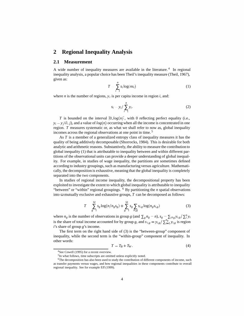
A wide number of inequality measures are available in the literature. 4 In regionalinequality analysis, a popular choice has been Theil’s inequality measure (Theil, 1967),given as:

T =n

∑i=1

si log(nsi) (1)

where n is the number of regions, yi is per capita income in region i, and:

si = yi=n

∑i=1

yi: (2)

T is bounded on the interval [0; log(n)], with 0 reflecting perfect equality (i.e.,yi = y j8i; j), and a value of log(n) occurring when all the income is concentrated in oneregion. T measures systematic or, as what we shall refer to now as, global inequalityincomes across the regional observations at one point in time. 5

As T is a member of a generalized entropy class of inequality measures it has thequality of being additively decomposable (Shorrocks, 1984). This is desirable for bothanalytic and arithmetic reasons. Substantively, the ability to measure the contribution toglobal inequality (1) that is attributable to inequality between and within different par-titions of the observational units can provide a deeper understanding of global inequal-ity. For example, in studies of wage inequality, the partitions are sometimes definedaccording to industry groupings, such as manufacturing versus agriculture. Mathemati-cally, the decomposition is exhaustive, meaning that the global inequality is completelyseparated into the two components.

In studies of regional income inequality, the decompositional property has beenexploited to investigate the extent to which global inequality is attributable to inequality“between” or “within” regional groupings. 6 By partitioning the n spatial observationsinto ω mutually exclusive and exhaustive groups, T can be decomposed as follows:

T =ω

∑g=1

sg log(n=ngsg)+ω

∑g=1

sg ∑i2g

si;g log(ngsi;g) (3)

where ng is the number of observations in group g (and ∑g ng = n), sg = ∑i2g yi;g=∑ni yi

is the share of total income accounted for by group g, and s i;g = yi;g=∑ngi=1 yi;g is region

i’s share of group g’s income.The first term on the right hand side of (3) is the “between-group” component of

inequality, while the second term is the “within-group” component of inequality. Inother words:

T = TB +TW : (4)4See Cowell (1995) for a recent overview.5In what follows, time subscripts are omitted unless explicitly noted.6The decomposition has also been used to study the contribution of different components of income, such

as transfer payments versus wages, and how regional inequalities in these components contribute to overallregional inequality. See for example Eff (1999).

4

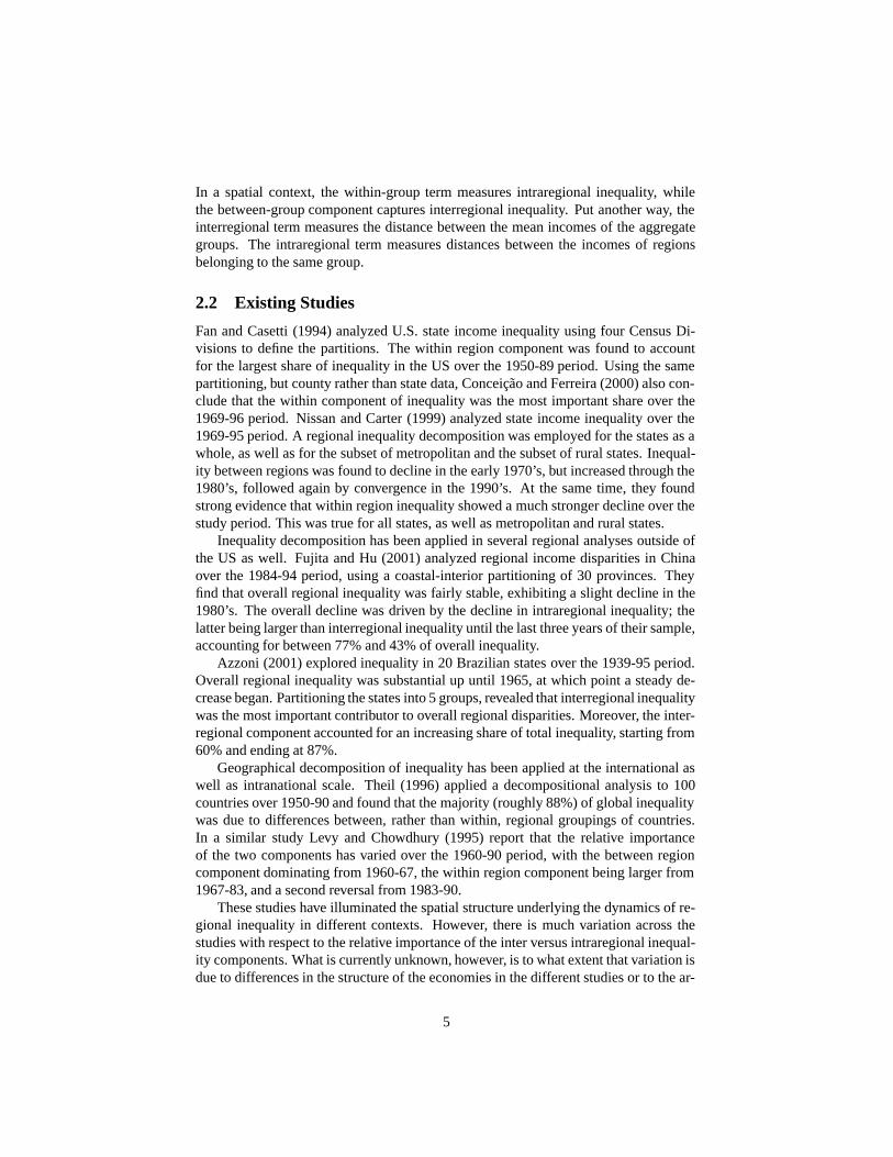
In a spatial context, the within-group term measures intraregional inequality, whilethe between-group component captures interregional inequality. Put another way, theinterregional term measures the distance between the mean incomes of the aggregategroups. The intraregional term measures distances between the incomes of regionsbelonging to the same group.

2.2 Existing Studies

Fan and Casetti (1994) analyzed U.S. state income inequality using four Census Di-visions to define the partitions. The within region component was found to accountfor the largest share of inequality in the US over the 1950-89 period. Using the samepartitioning, but county rather than state data, Conceicao and Ferreira (2000) also con-clude that the within component of inequality was the most important share over the1969-96 period. Nissan and Carter (1999) analyzed state income inequality over the1969-95 period. A regional inequality decomposition was employed for the states as awhole, as well as for the subset of metropolitan and the subset of rural states. Inequal-ity between regions was found to decline in the early 1970’s, but increased through the1980’s, followed again by convergence in the 1990’s. At the same time, they foundstrong evidence that within region inequality showed a much stronger decline over thestudy period. This was true for all states, as well as metropolitan and rural states.

Inequality decomposition has been applied in several regional analyses outside ofthe US as well. Fujita and Hu (2001) analyzed regional income disparities in Chinaover the 1984-94 period, using a coastal-interior partitioning of 30 provinces. Theyfind that overall regional inequality was fairly stable, exhibiting a slight decline in the1980’s. The overall decline was driven by the decline in intraregional inequality; thelatter being larger than interregional inequality until the last three years of their sample,accounting for between 77% and 43% of overall inequality.

Azzoni (2001) explored inequality in 20 Brazilian states over the 1939-95 period.Overall regional inequality was substantial up until 1965, at which point a steady de-crease began. Partitioning the states into 5 groups, revealed that interregional inequalitywas the most important contributor to overall regional disparities. Moreover, the inter-regional component accounted for an increasing share of total inequality, starting from60% and ending at 87%.

Geographical decomposition of inequality has been applied at the international aswell as intranational scale. Theil (1996) applied a decompositional analysis to 100countries over 1950-90 and found that the majority (roughly 88%) of global inequalitywas due to differences between, rather than within, regional groupings of countries.In a similar study Levy and Chowdhury (1995) report that the relative importanceof the two components has varied over the 1960-90 period, with the between regioncomponent dominating from 1960-67, the within region component being larger from1967-83, and a second reversal from 1983-90.

These studies have illuminated the spatial structure underlying the dynamics of re-gional inequality in different contexts. However, there is much variation across thestudies with respect to the relative importance of the inter versus intraregional inequal-ity components. What is currently unknown, however, is to what extent that variation isdue to differences in the structure of the economies in the different studies or to the ar-

5

ticulation of methodological issues across the studies. These issues include the choiceof regional partitioning and the spatial scale of the observational units.

At the same time, there are several limitations in these studies having to do with alack of an inferential basis that require additional attention. Moreover, it is possible thatmuch more can be said about the geographical dimensions of regional inequality. Inthe remainder of the paper, these issues are more fully discussed and an initial attemptat addressing these concerns is presented.

3 Spatial Effects in Regional Inequality Analysis

3.1 Spatial Dependence

Spatial dependence occurs when the values for some phenomenon measured at onelocation are associated with the values measured at other locations (Anselin, 1988).The issues that spatial dependence raise for econometric analysis of regional incomeconvergence have received recent attention (Fingleton, 2001; Rey and Montouri, 1999),yet the role of spatial dependence in studies of regional inequality has been largelyignored.

The issues associated with spatial dependence may be conveniently split into twogroups. From a substantive perspective, spatial dependence can play an important rolein shaping the geographical distribution of incomes. From a nuisance perspective,spatial dependence can complicate the application of traditional statistical methods de-signed to analyze regional inequality.

Lucas (1993) suggests a model that allows for cross-economy interactions in theform of human capital spillovers. The presence of these spillovers (i.e., learning bydoing) can radically alter the patterns of cross-economy growth from those suggestedby a traditional neoclassical growth model. The basic idea is that if economies interactvia human capital spillovers, and if the interacting economies become grouped, it islikely that within group spillovers will be stronger than between group spillovers. Thiswould result in within group convergence but, potentially, divergence between groups.

From a nuisance perspective, the presence of spatial dependence presents a chal-lenge to the use of statistical inference in inequality analysis. This is because the exist-ing approaches to inference are based on an assumption of random sampling which isviolated by the presence of spatial dependence. This issue is taken up further below.

Spatial dependence of a nuisance form can also arise from a mismatch between theregional boundaries used to organize the data and the boundaries of the actual socioe-conomic process under study. In regional inequality analysis, this could be reflected ina misspecified partitioning, whereby the partitioning imposed by the researcher fails tomatch the natural groupings of the regional observations.

Interestingly, global inequality measures are insensitive to the underlying spatialdistribution of the income values. This reflects a focus on the dispersion of the distribu-tion only. This also brings up an intriguing question regarding the relationship betweenthe level of spatial dependence in regional incomes and spatial income inequality. Atfirst glance, it would appear that strong positive spatial autocorrelation would lead toincreasing global inequality, given that we would be able to see clusters of similar

6

incomes on a map. However, the analysis of spatial autocorrelation rests on the as-sumption of spatial stationarity. Loosely speaking, this requires the mean and varianceof the distribution to be constant over space. At the same time, it is well known, thatthe presence of spatial dependence can induce a form of heteroskedasticity in the er-ror terms of spatial econometric models (Anselin, 1988). The question then becomesone of being able to disentangle any apparent spatial heterogeneity induced by the de-pendence, from true heterogeneity reflecting a lack of spatial stationarity. This wouldallow one to distinguish between increasing inequality owing to increasing variance ina distribution versus inequality attributable to the mixing of different distributions.

3.2 Spatial Scale in Regional Convergence Analysis

As is well known in other areas of spatial analysis, the modifiable areal unit problem(MAUP) arises when the inferences drawn about the process under study are sensitiveto the spatial scale and partitioning of the data at hand (Opensaw and Alvanides, 1999).Given the wide scope for selecting a spatial partitioning as well as the unit of observa-tion in regional inequality analysis, it would appear that the MAUP would attract muchattention. This, however, has not been the case.

That inequality measures will be subject to the MAUP can be seen by an exami-nation of the bounds for the the global T . The theoretical upper bound of T is log(n).Any change in spatial scale, say from the state level to the county level, will changethe number of observational units and affect the upper bound of the statistic. The ques-tion of how this affects the comparison of inferences drawn about inequality at the twodifferent scales has gone unexamined in the literature.

In addition to affecting the upper bound of the global T , a change in spatial scalemay also impact the decomposition of the global measure into its intra and interregionalcomponents. Here again, this issue has been neglected in previous regional studies.These issues are taken up in the empirical analysis in section 4.

3.3 Inferential Issues

In regional applications of inequality measures the focus is typically on a descriptiveanalysis, either reporting the value of the measure at one point in time, tracking thestatistic over time, or decomposing global regional inequality into its intra and interre-gional shares. An important omission in the regional literature is the use of inferentialmethods that allow for formal hypotheses testing regarding inequality measures. Sev-eral interesting hypotheses regarding regional inequality that could be examined froman inferential perspective:

� Is the coefficient different from what would be expected under perfect regionalequality

� Is any empirical change in an inequality measure over time significantly differentfrom zero?

� Is the share of intraregional inequality significantly different from some hypoth-esized value?

7

� In comparing two (or more) economic systems over time (i.e., the U.S. vs. theEU) is the difference in regional inequality significant?

� Are the within and between regional inequality components significantly differ-ent between the two systems?

In the wider inequality literature, two general approaches towards inference havebeen used. The first rests on theoretical results regarding the asymptotic distributionsof different inequality statistics (Maasoumi, 1997). Application of these results to thesmall samples used in most regional settings is problematic for two main reasons. First,the inequality statistics are typically truncated at 0. Use of asymptotic standard errors toconstruct confidence intervals around the empirical value for the statistic may produceinadmissible interval bounds. The second problem is that the small sample propertiesof these statistics are unknown, and as such the usefulness of asymptotic results is alsounknown.

The second approach to inference in inequality analysis rests on computationalprocedures. Mills and Zandvakili (1997) suggest the use of a bootstrap to constructempirical sampling distributions for inequality measures. At first glance, this mayappear to offer a way to introduce an inferential component into regional inequalityanalysis. Unfortunately, regional income data often displays a high degree of spatialautocorrelation (Rey and Montouri, 1999). The presence of such dependence violatesthe random sampling assumption at the heart of the bootstrap methodology. A similardifficulty applies to the asymptotic results.7

Because the presence of spatial dependence rules out the use of asymptotics orbootstrapping, an alternative approach to inference is required. The approach suggestedhere is based on random spatial permutations of the actual incomes for a given mappattern. This can be used to test hypotheses regarding the decomposition of globalinequality into its interregional and intraregional components. This is accomplishedwith the following steps:

1. Calculate decomposition:T � = T �

W +T �

B (5)

2. Randomly reassign incomes to new locations

3. Calculate decomposition for permutated map:

T P = T PW +T P

B (6)

4. Repeat steps 2 and 3, K times.

The values for the global inequality measure T P will be the same for any permu-tation in a given time period. Because the observations are being randomly reassigned

7In testing for changes in personal income inequality indices overtime the two temporal samples may bedependent, since the same individuals may be included in both periods. The focus here is on testing a singleregional distribution at one point in time, so this issue is not addressed. For further details see Zheng andCushing (2001).

8

to different regional groupings in each permutation, however, the values for the in-traregional (T P

W ) and interregional (T PB ) are likely to vary across the permutations. The

actual inequality measure T �

W can then be compared against the value it would havebeen expected to take on if regional incomes were randomly distributed in space. Thelatter would be obtained as the average of the empirically generated measures fromstep 3:

TW =1K

K

∑P=1

T PW (7)

Differences between the actual statistic and its expected value could be comparedagainst the empirical sampling distribution in one of two ways. The first would bebased on the assumption that the empirical sampling distribution is approximately nor-mal, in which case the standard deviation for that distribution, given as:

sTW =1K

K

∑P=1

�T P

W � TW�2

(8)

could be used to define a confidence interval.The second approach to inference using the random spatial permutations is to use

a percentile approach. This simply sorts the empirically generated T PW values and then

develops a pseudo significance level by calculating the share of the empirical valuesthat are more extreme than the actual value:

p(TW ) =1K

K

∑P=1

ψP (9)

where ψP = 1 if T PW is more extreme than TW , ψP = 0 otherwise. The advantage of this

approach over the first is that the problem of inadmissible interval bounds is avoided.Because the global inequality measure is invariant to the spatial arrangement of

regional incomes, the random permutation approach cannot be used to test inferencesregarding the global measure. Future work will focus on developing methods of infer-ence for the global measure in the presence of spatial dependence.

4 Empirical Illustration

To explore some of these issues we focus on US per capita income over the 1929-2000 period for the 48 lower states.8 Attention is first directed towards the relationshipbetween regional income inequality and spatial dependence. This is followed by ananalysis of how changes in spatial scale may affect the measures of regional inequality.Finally, approaches to statistical inference in regional inequality analysis are exam-ined.9

8The state and county income data used in this study were obtained from the May 3, 2001 release of theBEA state and local personal income series.

9The empirical analysis was carried out using the package STARS (Rey, 2001).

9

4.1 Inequality and Spatial Dependence

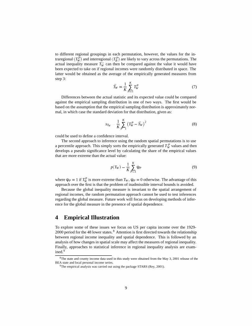
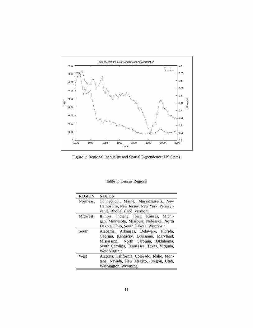
Figure 1 portrays the relationship between regional inequality and spatial autocorrela-tion. Inequality is measured using the global T from (1). Clearly, the long term trendhas been one of declining regional income inequality in the U.S., with the majorityof the decline coming during the war years in the early 1940’s. A slight turn aroundtowards increasing regional inequality is seen through the 1980’s, for which numerousexplanations have been put forth (Amos, 1988; Fan and Casetti, 1994). However, theseexplanations focus on US specific causes and ignore presence of a similar turn aroundin other national systems occurring during the same period. (Paci and Pigliaru, 1997).

Spatial autocorrelation is measured using Moran’s I, defined as:

I =n

∑i ∑ j wi; j

∑i ∑ j (yi� y)(y j� y)

∑i (yi� y)2 (10)

where wi; j is an element of a binary spatial contiguity matrix with elements taking onthe value of 1 if states i and j are first order neighbors (i.e., share a border), 0 otherwise.yi is per capita income in state i and y is the average per capita income for the 48 states.

Moran’s I has an expected value and variance that are function of the structure of thespatial weights matrix only, and are not influenced by the value of the variate in ques-tion. As such the moments of I are constant each year: E[I] =�0:213, V [I] = 0:009. 10

Basing inference regarding I on a normality assumption results in the statistic beingsignificant in each year in this sample. Thus, personal incomes are highly autocorre-lated across the states.

Figure 1 also reveals a strong positive relationship between the inequality measureand the autocorrelation index. The sample correlation between these two statistics overthe 72 years is 0.798. It should be noted, however, that a simple re-shuffling of the ac-tual income values about the map for a given year would leave the measure of inequal-ity unchanged, while Moran’s I would vary. This highlights the difference in emphasisbetween the two statistics and suggests that their joint application to the analysis ofregional income growth might produce important complementarities offering insightsnot obtainable when either is used in isolation.

Figure 2 displays the global T and its decomposition into the interregional andintraregional components. The partitioning of the 48 states is based on the US CensusRegions which are defined in Table 1. This is the same partitioning as used in Fan andCasetti (1994), although our sample includes a larger number of years. In each of the72 years, the intraregional component exceeds that of the interregional share. Theseresults are in agreement with those reported by Fan and Casetti (1994).

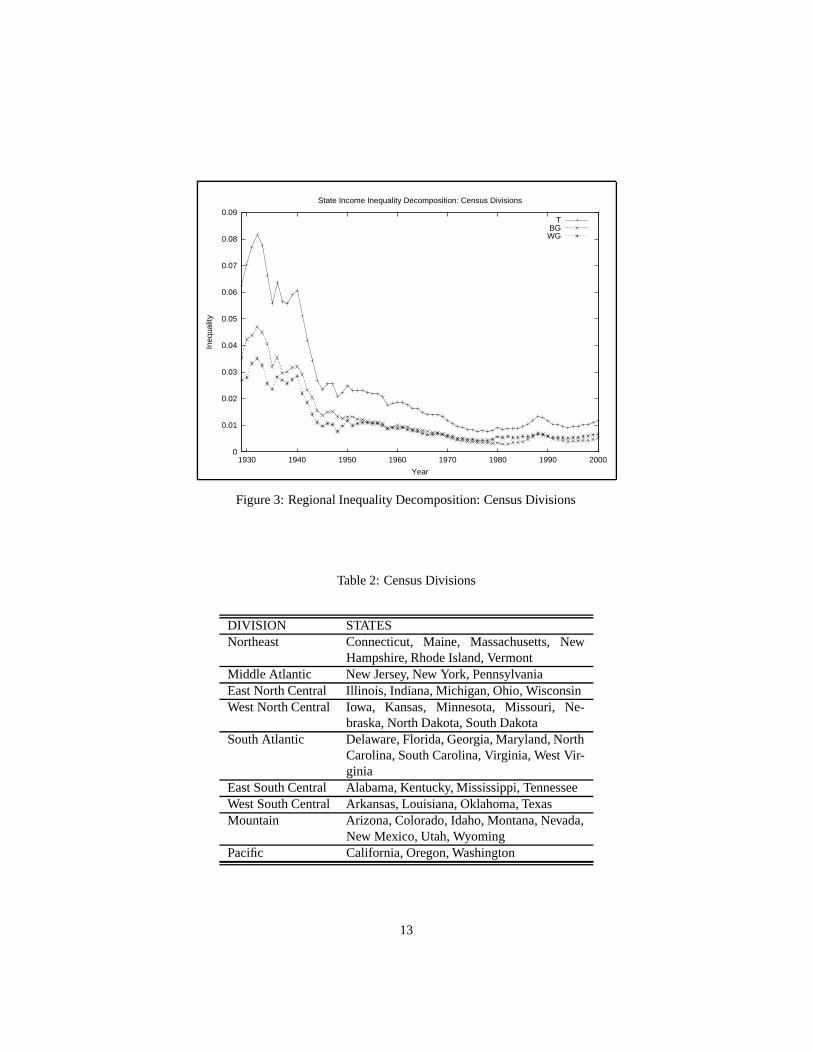
Figure 3 shows the effect of changing the partitioning scheme from the four Censusregions to the nine Census Divisions, as defined in Table 2. The relative importanceof the two components of inequality is reversed, with the interregional component nowdominating. This reflects an increase in the internal homogeneity of the regions, largelydue to the decrease in the number of states found in each region.

10For the detailed expressions for the moments of I under the normality assumption see Cliff and Ord(1973).

10

0

0.01

0.02

0.03

0.04

0.05

0.06

0.07

0.08

0.09

1930 1940 1950 1960 1970 1980 1990 20000.2

0.25

0.3

0.35

0.4

0.45

0.5

0.55

0.6

0.65

0.7T

heil

T

Mor

an’s

I

Year

State Income Inequality and Spatial Autocorrelation

TI

Figure 1: Regional Inequality and Spatial Dependence: US States

Table 1: Census Regions

REGION STATESNortheast Connecticut, Maine, Massachusetts, New

Hampshire, New Jersey, New York, Pennsyl-vania, Rhode Island, Vermont

Midwest Illinois, Indiana, Iowa, Kansas, Michi-gan, Minnesota, Missouri, Nebraska, NorthDakota, Ohio, South Dakota, Wisconsin

South Alabama, Arkansas, Delaware, Florida,Georgia, Kentucky, Louisiana, Maryland,Mississippi, North Carolina, Oklahoma,South Carolina, Tennessee, Texas, Virginia,West Virginia

West Arizona, California, Colorado, Idaho, Mon-tana, Nevada, New Mexico, Oregon, Utah,Washington, Wyoming

11

0

0.01

0.02

0.03

0.04

0.05

0.06

0.07

0.08

0.09

1930 1940 1950 1960 1970 1980 1990 2000

Ineq

ualit

y

Year

State Income Inequality Decomposition: Census Regions

TBGWG

Figure 2: Regional Inequality Decomposition: Census Regions

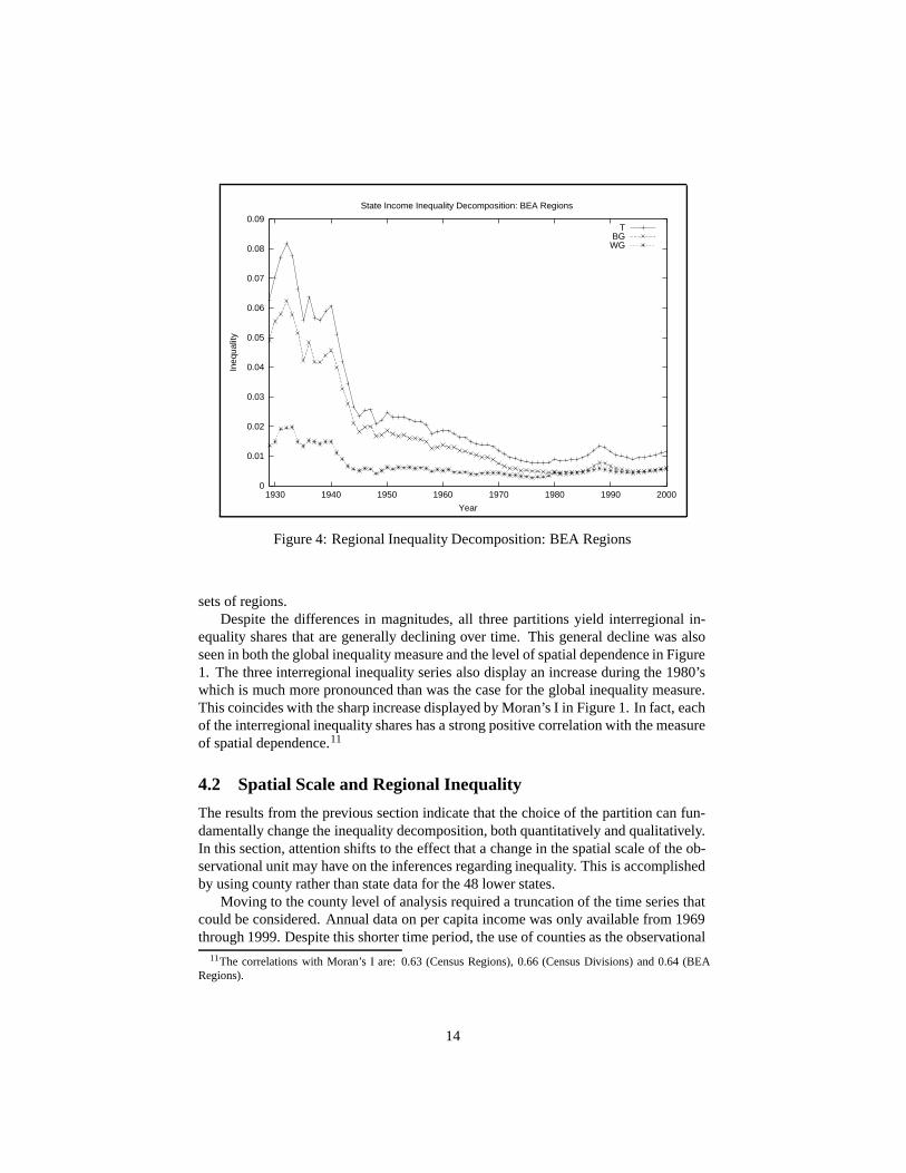
Figure 4 shows the effect of changing the partitioning scheme to the eight regionsdefined by the Bureau of Economic Analysis (BEA) and listed in Table 3. The rever-sal in the relative importance of the two components of inequality is even more pro-nounced. Although there is a high degree of similarity between the Census Divisionsand the BEA Regions, the interregional inequality component is substantially higherin the latter partitioning. Moreover, the share claimed by the interregional componentusing the BEA Regions in the first half of the study period is higher than that claimedby the intraregional component during the same period when the Census Divisions areused.

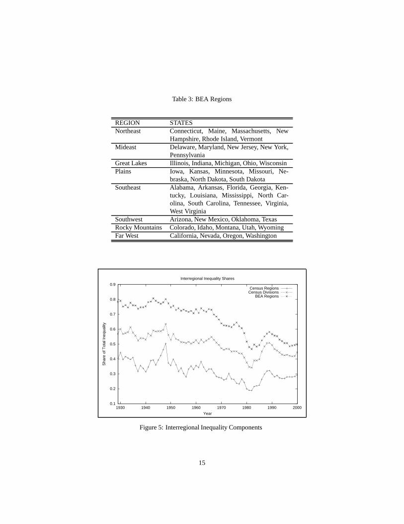
These interregional components are isolated in Figure 5 revealing the much higherinterregional share each year in the sample when the partitioning is based on the BEAregions. The larger number of groups in the BEA Regions and Census Divisions rela-tive to the Census Regions explains why the former have larger interregional compo-nents than the latter. However, the BEA Regions have higher interregional inequalitythan the Census Divisions, despite having a smaller number of groups of states. Con-sequently, the interregional share is not a simple function of the number of regionalgroupings used.

The rankings of the three partitions with respect to the share of total inequalityclaimed by the interregional component is consistent across the entire 72 year period,with the BEA scheme at the top and the Census Region partition at the bottom. Becausean increase in the interregional inequality is due to differences in the mean valuesbecoming more important than intraregional differences, the patterns in figure 5 suggestthat the homogeneity of the BEA regions is stronger than that found in the other two

12

0

0.01

0.02

0.03

0.04

0.05

0.06

0.07

0.08

0.09

1930 1940 1950 1960 1970 1980 1990 2000

Ineq

ualit

y

Year

State Income Inequality Decomposition: Census Divisions

TBGWG

Figure 3: Regional Inequality Decomposition: Census Divisions

Table 2: Census Divisions

DIVISION STATESNortheast Connecticut, Maine, Massachusetts, New

Hampshire, Rhode Island, VermontMiddle Atlantic New Jersey, New York, PennsylvaniaEast North Central Illinois, Indiana, Michigan, Ohio, WisconsinWest North Central Iowa, Kansas, Minnesota, Missouri, Ne-

braska, North Dakota, South DakotaSouth Atlantic Delaware, Florida, Georgia, Maryland, North

Carolina, South Carolina, Virginia, West Vir-ginia

East South Central Alabama, Kentucky, Mississippi, TennesseeWest South Central Arkansas, Louisiana, Oklahoma, TexasMountain Arizona, Colorado, Idaho, Montana, Nevada,

New Mexico, Utah, WyomingPacific California, Oregon, Washington

13

0

0.01

0.02

0.03

0.04

0.05

0.06

0.07

0.08

0.09

1930 1940 1950 1960 1970 1980 1990 2000

Ineq

ualit

y

Year

State Income Inequality Decomposition: BEA Regions

TBGWG

Figure 4: Regional Inequality Decomposition: BEA Regions

sets of regions.Despite the differences in magnitudes, all three partitions yield interregional in-

equality shares that are generally declining over time. This general decline was alsoseen in both the global inequality measure and the level of spatial dependence in Figure1. The three interregional inequality series also display an increase during the 1980’swhich is much more pronounced than was the case for the global inequality measure.This coincides with the sharp increase displayed by Moran’s I in Figure 1. In fact, eachof the interregional inequality shares has a strong positive correlation with the measureof spatial dependence.11

4.2 Spatial Scale and Regional Inequality

The results from the previous section indicate that the choice of the partition can fun-damentally change the inequality decomposition, both quantitatively and qualitatively.In this section, attention shifts to the effect that a change in the spatial scale of the ob-servational unit may have on the inferences regarding inequality. This is accomplishedby using county rather than state data for the 48 lower states.

Moving to the county level of analysis required a truncation of the time series thatcould be considered. Annual data on per capita income was only available from 1969through 1999. Despite this shorter time period, the use of counties as the observational

11The correlations with Moran’s I are: 0.63 (Census Regions), 0.66 (Census Divisions) and 0.64 (BEARegions).

14

Table 3: BEA Regions

REGION STATESNortheast Connecticut, Maine, Massachusetts, New

Hampshire, Rhode Island, VermontMideast Delaware, Maryland, New Jersey, New York,

PennsylvaniaGreat Lakes Illinois, Indiana, Michigan, Ohio, WisconsinPlains Iowa, Kansas, Minnesota, Missouri, Ne-

braska, North Dakota, South DakotaSoutheast Alabama, Arkansas, Florida, Georgia, Ken-

tucky, Louisiana, Mississippi, North Car-olina, South Carolina, Tennessee, Virginia,West Virginia

Southwest Arizona, New Mexico, Oklahoma, TexasRocky Mountains Colorado, Idaho, Montana, Utah, WyomingFar West California, Nevada, Oregon, Washington

0.1

0.2

0.3

0.4

0.5

0.6

0.7

0.8

0.9

1930 1940 1950 1960 1970 1980 1990 2000

Sha

re o

f Tot

al In

equa

lity

Year

Interregional Inequality Shares

Census RegionsCensus Divisions

BEA Regions

Figure 5: Interregional Inequality Components

15

0.05

0.1

0.15

0.2

0.25

0.3

0.35

0.4

0.45

1970 1975 1980 1985 1990 1995

Sha

re o

f Tot

al In

equa

lity

year

Interregional Inequality : Counties

StatesBEA

Census DivsionsCensus Regions

Figure 6: Interregional Inequality: County Unit of Observation

units has two important benefits. First, it vastly increases the number of spatial units,from 48 states to 3079 counties. The second benefit is that a fourth level of partitioningcan now be used, as the counties can be assigned to their states, while the states arenested in the three partitions examined in the previous section.

Figure 6 plots the interregional inequality shares for the counties using these fourpartitions. The most striking pattern is the substantially higher share found for the statepartition compared to those for the other three. Intuitively, this reflects the strongerhomogeneity of the states. The relative ranking of the three other partition is in gen-eral agreement with that found when the states were the unit of analysis, although thepattern is less clear from 1995 onward.

An important difference between the state and county level analysis is that the in-traregional inequality component dominates the global decomposition at the countyscale. This is true for all of the four partitions. When using the states as the unit of ob-servation, the only partition for which the intraregional component was the largest eachyear was the Census Regions (see Figure 5). For the BEA regions and Census Divi-sions, the interregional share was the largest for the majority of the years, again usingstates. If the focus is on the post-1969 period, the interregional component remainsdominant for the states only for the BEA regions partition.

4.3 Inference

The final issue examined is the role of inference in regional inequality analysis. Thisis an important issue as often interests centers on how much inequality the particular

16

decomposition accounts for. Cowell and Jenkins (1995) suggest a simple measure toget at this question:

R(B) = TB=T (11)

where TB and T are as defined above, and R(B) is the share of inequality accountedfor by the between group component. This is similar to the polarization index recentlysuggested by Zhang and Kanbur (2001):

P = TB=TW (12)

Unfortunately, neither of these studies developed an inferential basis against which themeasures could be evaluated, and instead used their measure in a descriptive fashion.

At this point, it could be asked why inference is needed, since the dominance of onecomponent over the other is sometimes readily apparent; for example the interregionalcomponent for the states using the Census Region partition is dominated by the in-traregional share (See Figure 2). The response is that this question misses an importantpoint. Finding that the interregional component accounts for a smaller share of globalinequality should not be taken to mean that the interregional component is irrelevant,or that the partition that it is based upon is somehow erroneous. The question shouldinstead be rephrased as follows: “For a given partition and spatial scale of observation,is the interregional share observed different from what could be expected by randomchance?”

Figure 7 provides an answer to this question. It depicts the actual value of the inter-regional inequality component for the states using the Census Regions as the partition.Also shown are the error bars associated with �2 standard deviations around the aver-age values for the shares from 1,000 random spatial permutations of the incomes foreach year. In each year of the sample, the interregional share is significantly greaterthan what would be expected if incomes were randomly distributed in space. This re-sult is of particularly interest, as it was the Census Regions partition that had a smallerinterregional share relative to its intraregional share. By extending the traditional de-compositional analysis to include an inferential component we find that, although thisinterregional inequality component is relatively small, the Census Regions do capturesome aspect of spatial structure. Without the inferential test, this partition might havebeen viewed as irrelevant or misspecified given that the interregional share was foundto be stronger in the other partitions.

5 Conclusion

In their overview of recent empirical work on economic growth Durlauf and Quah(1999) conclude that the field remains in its infancy (pg. 295). One sign of increas-ing maturity is the recent attention given to the geographical dimensions of economicgrowth (Barro and Sala-i-Martin, 1991; Krugman, 1991; Nijkamp and Poot, 1998).Application of recently developed methods of spatial econometrics to the question ofregional convergence has yielded a more comprehensive and multidimensional view ofregional economic growth (Goodchild et al., 2000).

17

-0.1

0

0.1

0.2

0.3

0.4

0.5

0.6

1930 1940 1950 1960 1970 1980 1990 2000

Ineq

ualit

y S

hare

Year

Simulated Versus Actual Interregional Inequality: Census Regions

Actual ShareSimulated

Figure 7: Simulated Versus Actual Interregional Inequality, Census Regions: StateUnit of Observation

The literature on regional income inequality, although somewhat older than theconvergence literature, has been slower to adopt new spatially explicit methods of dataanalysis. This chapter has attempted to contribute to such an adoption by investigatingthe role of spatial dependence and spatial scale in the analysis of regional income in-equality in the US over the 1929-2000 period. The key findings include with regard tospatial dependence include:

� A strong positive relationship between measures of inequality in state incomesand the degree of spatial autocorrelation.

� A strong positive relationship between the interregional inequality share (as op-posed to intraregional inequality) and spatial clustering.

The analysis of the role of the spatial scale of the observational unit and the choiceof regional partitioning of the units revealed the following:

� The qualitative and quantitative results of inequality decomposition are highlysensitive to the scale of the observational unit. Interregional inequality is dom-inant when state data are used, yet intraregional inequality is most importantwhen county level data are used.

� The relative importance of the interregional inequality component is not a simplefunction of the number of groups used in a partitioning of the regional observa-tions.

18

Finally, the study also suggested an approach to inference in the decompositionalanalysis of regional income inequality, offering an important complement to the exist-ing literature that has relied exclusively on descriptive methods.

19

References

Alonso, W. (1980). Five bell shapes in regional development. Papers of the RegionalScience Association, 45:5–16.

Amos, Jr, O. (1983). The relationship betwen personal income inequality, regionalincome inequality, and development. Regional Science Perspectives, 13:3–14.

Amos, Jr, O. (1988). Unbalanced regional growth and regional income inequality in thelatter stages of development. Regional Science and Urban Economics, 18:549–566.

Anselin, L. (1988). Spatial Econometrics: Methods and Models. Kluwer, Boston.

Armstrong, H. and Vickerman, R. (1995). Convergence and Divergence Among Euro-pean Regions. Pion, London.

Azzoni, C. R. (2001). Economic growth and income inequality in Brazil. Annals ofRegional Science, 31(1):133–152.

Baker, J. L. and Grosh, M. E. (1994). Measuring the effects of geographic targeting onpoverty reduction. World Bank Living Standards Measurement Study.

Barro, R. and Sala-i-Martin, X. (1991). Convergence across states and regions. Brook-ings papers on Economic Activity, 1:107–182.

Chatterji, M. and Dewhurst, J. (1996). Convergence clubs and relative economic per-formance in Great Britan. Regional Studies, 30:31–40.

Cliff, A. and Ord, J. (1973). Spatial Autocorrelation. Pion, London.

Conceicao, P. and Ferreira, P. (2000). The young person’s guide to the Theil index:suggesting intuitive interpretations and exploring analytical applications. Universityof Texas Inequality Project Working Paper 14.

Cowell, F. A. (1995). Measuring Inequality. Prentice Hall, London.

Cowell, F. A. and Jenkins, S. P. (1995). How much inequality can we explain? Method-ology and an application to the United States. The Economic Journal, 105(429):421–430.

Cuadrado-Roura, J., Garcia-Greciano, B., and Raymond, J. (1999). Regional conver-gence in productivity and productivity structure: The Spanish case. InternationalRegional Science Review, 22:35–53.

Durlauf, S. N. and Quah, D. T. (1999). The new empirics of economic growth. InTaylor, J. B. and Woodford, M., editors, Handbook of Macroeconomics: Volume 1A,pages 235–308. Elsevier, Amsterdam.

Eff, E. A. (1999). Myrdal contra Ohlin: Accounting for sources of U.S. county percapita income convergence using a flexible decomposition approach. Review of Re-gional Studies, 29(1):13–36.

20

Fan, C. C. and Casetti, E. (1994). The spatial and temporal dynamics of US regionalincome inequality, 1950-1989. Annals of Regional Science, 28:177–196.

Fingleton, B. (1999). Estimates of time to economic convergence: An analysis ofregions of the Eurpean Union. International Regional Science Review, 22:5–35.

Fingleton, B. (2001). Regional economic growth and convergence: insights from aspatial econometric perspective. In Anselin, L. and Florax, R., editors, Advances inSpatial Econometrics. Springer-Verlag, Berlin.

Fujita, M. and Hu, D. (2001). Regional disparity in China 1985-1994: The effects ofglobalization and economic liberalization. Annals of Regional Science, 35:3–37.

Goodchild, M., Anselin, L., Applebaum, R., and Harthorn, B. H. (2000). Towards aspatially integrated social science. International Regional Science Review, 23:139–159.

Kanbur, R. and Zhang, X. (1999). Which regional inequality? The evolution of rural-urban and inland-coastal inequality in China, 1983-1995. Journal of ComparativeEconomics, 27:686–701.

Krugman, P. (1991). Geography and Trade. MIT Press, Cambridge.

Kuznets, S. (1955). Economic growth and income equality. American Economic Re-view, 45:1–28.

Levy, A. and Chowdhury, K. (1995). A geographical decomposition of intercountryincome inequality. Comparative Economic Studies, 37:1–17.

Lucas, R. E. (1993). Making a miracle. Econometrica, 61(2):251–271.

Maasoumi, E. (1997). Empirical analysis of inequality and welfare. In Pesaran, M.and Schmnidt, P., editors, Handbook of Applied Econometrics, Volume II, Microeco-nomics, pages 202–245. Blackwell Publishers Ltd., London.

Maxwell, P. and Peter, M. (1988). Income inequality in small regions: A study ofAustralian statistical divisions. The Review of Regional Studies, 18:19–27.

Mills, J. A. and Zandvakili, S. (1997). Statistical inference via bootstrapping for mea-sures of inequality. Journal of Applied Econometrics, 12(2):133–150.

Nijkamp, P. and Poot, J. (1998). Spatial perspectives on new theories of economicgrowth. Annals of Regional Science, 32:407–437.

Nissan, E. and Carter, G. (1999). Spatial and temporal metropolitan and nonmetropoli-tan trends in income inequality. Growth and Change, 30(3):407–415.

Opensaw, S. and Alvanides, S. (1999). Applying geocomputation to the anaylsis ofspatial distributions. In Longley, P., Goodchild, M., Maguire, D., and Rhind, D.,editors, Geographic Information Systems Volume I: Principles and Technical Issues,pages 267–282, New York. John Wiley.

21

Paci, F. and Pigliaru, F. (1997). Structural change and convergence: an Italian perspec-tive. Structural Change and Economic Dynamics, 8:297–318.

Rey, S. J. (2001). Space-time analysis of regional systems: STARS. Technical report,Department of Geography, San Diego State University.

Rey, S. J. and Montouri, B. D. (1999). U.S. regional income convergence: A spatialeconometric perspective. Regional Studies, 33:143–156.

Shorrocks, A. F. (1984). Inequality decomposition by population subgroups. Econo-metrica, 52(6):1369–1385.

Theil, H. (1967). Economics and Information Theory. North Holland, Amsterdam.

Theil, H. (1996). Studies in Global Econometrics. Kluwer Academic Publishers, Dor-drecht.

Tsui, K. Y. (1993). Decomposition of China’s regional inequalities. Journal of Com-parative Economics, 17:600–627.

Williamson, J. (1965). Regional inequality and the process of national development.Economic Development and Cultural Change, 4:3–47.

Zhang, X. and Kanbur, R. (2001). What difference do polarisation measures make? Anapplication to China. Journal of Development Studies, Forthcoming.

Zheng, B. and Cushing, B. J. (2001). Statistical inference for testing inequality indiceswith dependent samples. Journal of Econometrics, 101:315–335.

22