51
Spatial Data Mining in the Era of Big Data Dr. Jin Soung Yoo Associate Professor Department of Computer Science Indiana University-Purdue University Fort Wayne
| Date post: | 20-May-2018 |
| Category: |
Documents |
| Upload: | nguyenkhue |
| View: | 215 times |
| Download: | 2 times |

Spatial Data Mining in the Era of Big Data
Dr. Jin Soung Yoo Associate Professor Department of Computer Science Indiana University-Purdue University Fort Wayne

Outline
Introduction to Data Mining Works in Data Mining

What is Data Mining
A computer-assisted process of discovering interesting, previously unknown, implicit, potentially useful, and non-trivial patterns or knowledge from large databases Non-trivial search
Large (e.g., exponential) search space of plausible hypothesis Interesting
Useful in certain application domain Unexpected
Patterns is not common knowledge May provide a new understanding of world

With rapid advances in data collection and storage technology, the explosive growth of data from
many data sources Purchases at grocery stores,
customer services from call centers Web logs from e-commerce Web sties Bank/Credit card transactions Mobile phone contents Social networks World Wide Web: online news, digital
images, YouTube
Why Data Mining - Commercial Viewpoint
Source: various web sites

Why Data Mining (Conti.)
Competitive pressure
Today business environment requires critical data analysis Market analysis: targeted marketing, cross-selling,
market segments, etc. Risk management: forecasting, customer retention Fraud detection and detection of unusual behavior
Business questions “Who are the most profitable customers?” “What products can be cross-sold?” “How change if a new local store is added?”

Example: Target’s Finding
“Women on the baby registry were buying larger quantities of unscented lotion around the beginning of their second trimester. ”
Target has figured out whether you have a baby on the way long before you need to start buying diapers
“When someone suddenly starts buying lots of scent-free soap and extra-big bags of cotton balls, in addition to hand sanitizers and washcloths, it signals they could be getting close to their delivery date.”
Source: http://www.forbes.com/sites/kashmirhill/2012/02/16/how-target-figured-out-a-teen-girl-was-pregnant-before-her-father-did/

Why Data Mining - Scientific Viewpoint
Many science areas are collecting data for their new important discovery Earth observations from satellites
Climate measurement
Sloan Digital Sky Survey (SDDS)
Cancer/epidemic data (SEER)
Microarrays generating gene expression data
Scientific simulations
Animal behavior observation
Source: various web sites

Scale of Data
Organization Scale of Data
Walmart ~ 1 million customer transactions / hr Facebook ~ 50 billion photos
Yahoo ~48 GB Web log data/hr Falcon Credit Card Fraud Detection System (FICO)
2.1 billion active accounts world-wide
Business data worldwide, across all companies
Doubles every 1.2 years
NASA satellites ~ 1.2 TB/day Sloan Digital Sky Survey
(SDSS) ~140 TB
(200GB /night) NCBI GenBank ~ 22 million genetic sequences
Source: http://en.wikipedia.org/wiki/Big_data

Big Data but No Clue
There is often information “hidden” in the data that is not readily evident
Much of the data is never analyzed at all.
9
“The great strength of computers is that they can reliably manipulate vast amounts of data very quickly. Their great weakness is that they don’t have a clue as to what any of that data actually means” (Cass, IEEE Spectrum, Jan 2004)
source: http://shawnwhatley.com/

Picture source: www.exelanx.com
Data mining is the art of finding treasures in the sea of data when you don't know what you're looking for or what you might find.

Confluence of Multiple Disciplines
Data Mining
Database Technology
Statistics
Machine Learning
Pattern Recognition
Algorithm
Other Disciplines
Visualization
Artificial Intelligence

Data Mining for Many Other Disciplines
Picture source: amazon.com

Outline
Introduction to Data Mining Works in Data Mining Spatial Data Mining Spatial Association Mining in Cloud
Computing Environment Temporal Data Mining Spatiotemporal Data Mining Biological Data Mining Educational Data Mining

Spatial Data – Everywhere
Environmental Science
Earth Science
Public Health
Business (Location-Based Services)
Transportation
Evolution of Location aware devices, Mobile computing, Wireless network
Military, Homeland security
Criminology
*Pictures from various sources

Spatial Data Mining
The process of discovering interesting, useful, non-trivial (as “automatized” as possible) patterns from large spatial or spatiotemporal data.
Classification Clustering
Prediction
Association, Outlier
Interaction Hot spots
Prediction Colocation detection
Spatial Pattern Families vs. Techniques
* Pictures from various sources

Examples of Spatial Patterns
Spatial relationships (location, region, frontier, neighborhood, obstruction, field, basin, communication, diffusion, propagation) are importantly considered for the pattern discovery
Historic Examples 1855 Asiatic Cholera in London:
A water pump identified as the source
Fluoride and health gums near Colorado river (with originally insufficient amount of fluoride) * Street map of cholera
deaths in London Soho from John Snow in 1855
Source: http://en.wikipedia.org/wiki/1854_Broad_Street_cholera_outbreak

Examples of Spatial Patterns
Modern Examples Cancer clusters to locate hazardous environments Nile virus spreading from north east USA to south and west Crime hotspots for planning police patrol routes Colocation of a business with another franchise (such as
colocation of a Pizza Hut restaurant with a Blockbuster video store)
Best locations for opening new hospitals based on the population of patients who live in each neighborhood.
Spatial region-based personalization Unusual warming of Pacific ocean (El Niño) effects weather
in USA

Outline
Introduction to Data Mining Works in Data Mining Spatial Data Mining Spatial Association Mining
Spatial Association Mining in Cloud Computing Environment
Summary

Spatial Association, Co-location, Correlation
Spatial association mining discovers interesting spatial relationships and correlations among spatial objects. Spatial correlation (or, neighborhood influence) refers
to the phenomenon of the location of a specific object in an area affecting some nonspatial attribute of the object.
For example, the value (nonspatial attribute) of a house at a given address (geocoded to give a spatial attribute) is largely determined by the value of other houses in the neighborhood.

Spatial Co-location
M R
M
M R
R
M
R R
P
P
W
P R
P
R
N W
N
{ , }, Answer: Movie
Parking Restaurant { , } Restaurant
A co-location represents the presence of two or more spatial objects at the same location or at significantly close distances from each other.
Co-location mining finds all subsets of spatial events (/ features) which are frequently observed in nearby areas.
In the case of including non-spatial information For example, sales at franchises
of a specific pizza restaurant chain were higher at restaurants colocated with video stores than at restaurants not colocated with video stores.
Find patterns from the above sample dataset?

Co-location Examples
Domain Example Features Example Co-location Patterns
Which spatial events are related to each other? Which spatial phenomena depend on other phenomenon?
Epidemiology Disease types,
environmental events {West Nile disease, stagnant water sources, dead birds, mosquitoes}
Location-based services
Service type requests {tow truck, police, ambulance}
Business Local store types {Burger King, MacDonald’s}
Transportation Delivery service tracks {US Postal Service, UPS, newspaper delivery}
Military Critical points, events {weapons Caches, IED factories} Economics Industry types {suppliers, producers, consultants} Ecology Species {Nile crocodile, Egyptian plover} Earth Science
Climate and disturbance events
{wild fire, hot, dry, lightning}
Weather Fronts, precipitation {cold front, warm front, snow fall}
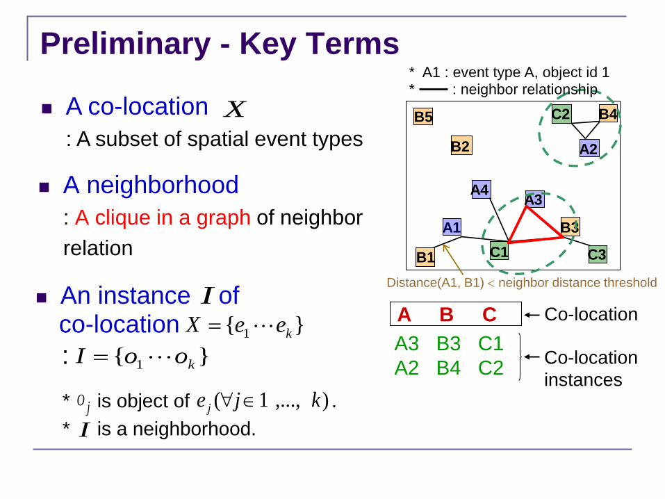
Preliminary - Key Terms
A neighborhood : A clique in a graph of neighbor relation
A co-location : A subset of spatial event types
X
A1
A3
B3
C3 C1
A4
B4
A2
B5
B2
B1
C2
A B C Co-location A3 B3 C1 A2 B4 C2 Co-location
instances
* : neighbor relationship * A1 : event type A, object id 1
Distance(A1, B1) < neighbor distance threshold An instance of
}{ 1 keeX =I
* is object of . ),...,1( kje j ∈∀jO
I * is a neighborhood.
co-location }{ 1 kooI =:

Preliminary - Interest Measures
A1
A3
B3
C3 C1
A4
B4
A2
B5
B2
B1
C2
A B C Co-location A3 B3 C1 A2 B4 C2
Co-location instances
Participation Ratio
i
i
eXe
ofobjectsof#ofinstancesinofobjectsof#
),( XePR i
2/4 2/5 PI
min( )
}{ 1 keeX =
)},({min)( XePRXPI iXei∈=
PI of co-location
If PI > prev_threshold, {A, B,C} is a frequent co-location.
* Strength of prevalence of co-location
* Strength of each event type in a co-location
Participation Index
PRs 2/5 2/3 : Participation ratio of A
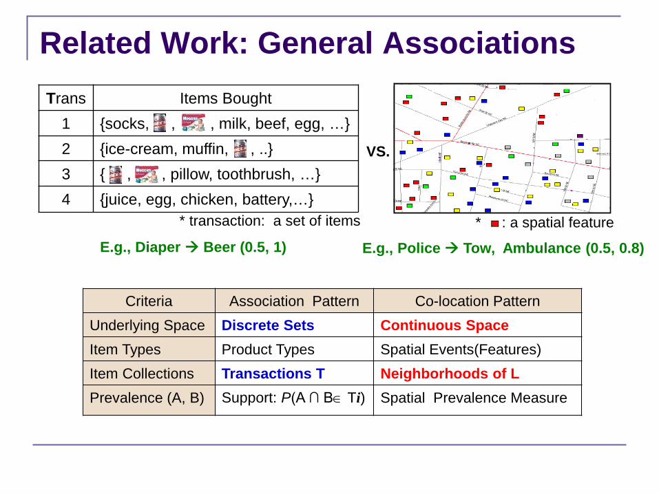
Related Work: General Associations
VS.
Trans Items Bought 1 {socks, , , milk, beef, egg, …} 2 {ice-cream, muffin, , ..} 3 { , , pillow, toothbrush, …} 4 {juice, egg, chicken, battery,…}
* transaction: a set of items
Criteria Association Pattern Co-location Pattern Underlying Space Discrete Sets Continuous Space Item Types Product Types Spatial Events(Features) Item Collections Transactions T Neighborhoods of L Prevalence (A, B) Support: P(A ∩ B∈ Ti) Spatial Prevalence Measure
* : a spatial feature
E.g., Diaper Beer (0.5, 1) E.g., Police Tow, Ambulance (0.5, 0.8)

M W S R KSR(d)
KMW(d)
Related Work: Statistical Approach
Limitations Not proper for analysis of features of size 3 e.g., triple features (K,T,R)
Not efficient in computation
≥
λ Ripley’s Cross K-Function [Cressie]
Kij(d) = j-1E [number of type j feature within distance d of a randomly chosen type i feature] .
Spatially correlated
Spatial complete randomness

Related Work: Colocation in Oracle

Challenges
No explicit transaction concept in spatial data Non-trivial to reuse association mining algorithms
Continuous neighbor relationship Especially, clique relations
Very large search space Given n features, there are
around 2n possible candidate feature sets
Other workload Density, neighbor distance,
prevalence threshold, etc.
Inherently too demanding of both processing time and memory requirements
null
AB AC AD AE BC BD BE CD CE DE
A B C D E
ABC ABD ABE ACD ACE ADE BCD BCE BDE CDE
ABCD ABCE ABDE ACDE BCDE
ABCDE

Why Not Use Modern Computational Framework Standard architecture emerging:
Cluster of commodity Linux nodes Gigabit Ethernet interconnect
Popular modern computational framework: Cloud computing (distributed computing over a
network) Hadoop (MapReduce), a software framework for
large-scale processing of data on clusters of commodity hardware.
How to organize the mining computations on this architecture?

Problem Formulation
Given A spatial event dataset, <id, event type, location> A spatial neighbor relationship (e.g., distance threshold) A prev_threshold
Objectives Develop a parallel/distributed co-location mining
algorithm for spatial association analysis in cloud computing environment.
Find Co-location patterns with participation index > prev_threshold

Outline
Introduction to Data Mining My Works in Data Mining Spatial Data Mining Spatial Association Mining in Cloud
Computing Environment Background: Hadoop and MapReduce Proposed Approach Experimental Evaluation
Summary

Background: Hadoop
Execution framework for running applications on large clusters of commodity hardware Includes Storage: HDFS Processing: MapReduce
Support the Map/Reduce programming model
Characteristics Economy: use cluster of commodity computers Easy to use
Users: no need to deal with the complexity of distributed computing
Reliable: can handle node failures automatically

Background: MapReduce
The hart of Hadoop A programming model for processing large data sets
with a parallel, distributed algorithm on a cluster. The term MapReduce actually refers to two separate and
distinct tasks that Hadoop programs perform. The first is the map job, which
takes a set of input data and converts it into another set of data.
The reduce job takes the output from a map as input and combines those data tuples into a smaller set of tuples.
Animation: http://www.systems-deployment.com/animation.html
Figure source: http://blog.sqlauthority.com/2013/10/09/big-data-buzz-words-what-is-mapreduce-day-7-of-21/

Example: Word Count on MapReduce A map function process a key/value pair to generate a set of
intermediate key/value pairs map(key=null, val=record):
For each word w in contents, emit (w, “1”) The shuffling step merges all intermediate values associated with the
same intermediate key and feed the key/values pairs to a reduce function. The reducer generates a set of result key/value pairs. reduce(key=word w, values=[1, 1, …,1]):
Sum all “1”s in values list Emit result (word, sum)
Figure source: http://www.alex-hanna.com/tworkshops/lesson-5-hadoop-and-mapreduce/

MapReduce Model is Widely Applicable
Example uses: distributed grep distributed sort web link-graph reversal term-vector / host web access log stats inverted index construction document clustering machine learning statistical machine translation ... ... ...
Source: http://research.google.com/archive/mapreduce-osdi04-slides/index-auto-0005.html/

Outline
Introduction to Data Mining My Works in Data Mining Spatial Data Mining Spatial Association Mining in Cloud
Computing Environment Background: Hadoop and MapReduce Proposed Approach Experimental Evaluation
Summary

Co-location Mining on MapReduce
<o_i, N(o_i)>
<o_i, N(o_i)>
Job1: Neighboring object search
<null, (o_i, o_j)> <grid no, o>
Job 2: Spatial neighborhood materialization
<o_i, o_j> <null, (o_i, o_j)>
<null, o>
Job 4: Co-located event set search
<eventset, instance>
<eventer, [instance]>
<co-located event set, prevalence> <o_i, N(o_i)>
Map
Collect size k candidate instance
Reduce
Filter true instance
Compute prevalence measures
Find prevalent co-located event sets
Neighborhood records
INPUT A spatial dataset
Map Reduce
Map
OUTPUT
Neighbor distance
prevalence threshold
Check neighbor constraints
Reduce
Search all neighboring pairs
Assign a grid no to data object
Neighbor pairs
Generate the neighborhood record
Shuffle and S
ort
<grid no, [o]>
<o_i, [o_j]>
{eventset, instance}
k=2 k=k+1
{size, prev event}
Job 3: Event object count
<event, 1 > <event, count> Map event=type of o_i
Reduce Count event objects
<event, [1]>
{event type, count} k=1
Shuffle and S
ort S
huffle and.. S
huffle and Sort
Drop unprevalent event objects in N
Preprocess
Co-location pattern mining
<o_i, N(o_i)>
Neighborhood records

Job1: Neighbor object search
Job1: Neighboring object search
<null, (o_i, o_j)> <grid no, o> <null, o>
INPUT A spatial dataset
Map Reduce
Neighbor distance
Search all neighboring
pairs
Assign a grid no to data object
Shuffle and Sort
<grid no, [o]>
Partition D
C4
B4
A3
C2 B2
B3
B5
C1
A2 A4
A1 B1 C3 d
d
d
Partition C
Partition A Partition B
Partition D
d d
1 A -85.1113430 41.1016631 2 A -85.1085207 41.1026886 1 B -85.1036761 41.1018515
… 4 C -85.1084791 41.1017347
(null, A1 B1) (null, A1 C1) (null, A2 B4) (null, A2 C2) …
Overlapping space partition Plane-sweep algorithm
O(nlogn)
(PartionD, 1 A -85.113430 41.1016631)
(PartionD, [1 A -85.113430 41.1016631, 2 A -85.1085207 41.1026886 …] )

Job2: Neighbor object search
<o_i, N(o_i)>
Job 2: Spatial neighborhood materialization
<o_i, o_j> <null, (o_i, o_j)> Map Check the neighbor
constraint o_i’s type < o_j’s type
Reduce Neighbor pairs
Generate the neighborhood
record
<o_i, [o_j]>
(null, A1 B1) (null, A1 C1) (null, A2 B4) (null, A2 C2) …
Job 1 Output
A3 B3 A3
C1
C1 B3
C3
A1
B3
B1 A1
C1
A4 A4 C1
A2 B4 A2
C2
B1
A1
C1 C3
B3
A3 A4
A2
B4 C2 B5
B2
B4 B4 C2
Pivot object Sub-star
(A1, (A1, B1, C1)) (A2, (A2, B4, C2)) (A3, (A3, B3, C1)) (A4, (A4, C1))
(B1, (B1)) (B2, (B2)) (B3, (B3, C1, C3)) (B4, (B4, C2)) (B5, (B4)) (C1, (C1)) (C2, (C2)) (C3, (C3))
Disjoint neighborhood partition
Conditional neighborhood transactions
Shuffle and Sort
CONCEPTUAL FIGURE for Job1 and Job2

Job3: Event Object Count (Optional)
Job 3: Event object count <event type,
1 > <event type, count> Map event=type of o_i
Reduce Count event objects
<event type, [1]>
{event type, count}
Shuffle and.. (A1, (A1, B1, C1))
(A2, (A2, B4, C2)) (A3, (A3, B3, C1)) (A4, (A4, C1))
(B1, (B1)) (B2, (B2)) (B3, (B3, C1, C3)) (B4, (B4, C2)) (B5, (B5))
(C1, (C1)) (C2, (C2)) (C3, (C3))
Job 2 Output
<o_i, N(o_i)>
Neighborhood records
(A , 4) (B , 5) (C , 3)

Job4: Prevalent Co-located Event Set Search
(A1, (A1, B1, C1)) (A2, (A2, B4, C2)) (A3, (A3, B3, C1)) (A4, (A4, C1))
(B1, (B1)) (B2, (B2)) (B3, (B3, C1, C3)) (B4, (B4, C2)) (B5, (B5)) (C1, (C1)) (C2, (C2)) (C3, (C3))
Job 2 Output
<o_i, N(o_i)>
Neighborhood records
<o_i, N(o_i)> Job 4: Co-located event set search
<eventset, instance>
<eventset, [instance]>
<co-located event set, prevalence>
Map
Collect size k candidate instance
Reduce
Filter true instance
Compute prevalence measures
Find prevalent co-located event sets
OUTPUT
prevalence threshold
{eventset, instance} A given pattern size K Or k=2 k=k+1
{size, prev event}
{event type, count}
Shuffle and S
ort
Drop unprevalent event objects in N
<{A, B, C}, [{A3, B3, C1}, {A2, B4, C2}]>
<{A, B, C}, {A3, B3, C1}, >
<{A, B}, 3/5> <{A, C}, 2/3> … <{A, B, C}, 2/5> …

Outline
Introduction to Data Mining My Works in Data Mining Spatial Data Mining Spatial Association Mining in Cloud
Computing Environment Background: Hadoop and MapReduce Proposed Approach Experimental Evaluation
Summary

Experimental Environment
For real resizable clusters, Amazon Web Services (AWS) Elastic MapReduce (EMR) platform
• Clusters with 1 ~ 20 nodes • Node type: m1.small (1 CPU, 1.7GB memory, 160GB storage), m1.large • Software: Hadoop 1.0.3, Hbase • Programming language:
Java, MapReduce API, Hbase API
* Source: Amazon AWS

0
200
400
600
800
1000
1200
1 3 6 12
Exec
utio
n tim
e (s
ec)
Number of of cluster nodes
EXP1-2 (30K points)EXP1-3 (50K points)EXP1-4 (70K points)
0
200
400
600
800
1000
1200
1 3 6 12
EXP1-4: f100p70K
Job3(Frequent set search)
Job2(Neigh. trans. generation)
Job1(Neighbor search)
Results with Synthetic Datasets
* For other results, please refer the paper in http://users.ipfw.edu/yooj/publication.html

050
100150200250300350400450500
1 3 6 12
Exec
utio
n tim
e (s
ec)
Number of cluster nodes
EXP5-1-2( Frequent set mining)EXP5-1-1(Preprocess)
Results with Real-world Datasets Theft incidents (5218 points) and
Point of interests (765 points, 16 types) in Fort Wayne area, and 1km for neighbor distance
Point of Interests in Washington D.C. (17000 points, 87 types)
0500
100015002000250030003500
1 5 10 20Number of nodes
distance=0.1 miledistance=0.15 miledistance=0.2 mile

Finding from Washington DC POI Data
Point of Interests in Washington D.C. (17000 points, 87 types), 0.2 mile for neighbor distance
{Bank, Pub, Restaurant} (0.4) {Bank, Café, Pub} (0.4) {Bank, Café, Fast Food Restaurant} (0.43) {Bank, Pub, Public pieces of art} (0.41) {Bank, Café, Hotel} (0.41) {Building, Café, Restaurant} (0.44) {Building, Café, Fast Food Restaurant}
(0.42) {Building, Restaurant, Fast Food
Restaurant} (0.42) …
{Pitch, Tennis} (0.7) {Museum, Public pieces of art} (0.55) {Park, Parking}(0.54) {Hostel, Recreation ground} (0.5) {Bicycle rental, Public pieces of art} (0.49) {Building, Parking} (0.48) {Attraction, Waste disposal} (0.46) {Bus Stop, Fast Food Restaurant} (0.44) {10-pin Blowing, Court house} (0.42) {Basketball, Tennis}(0.42) …

Visualization
Visualization of data points of selected 27 types Visualization of data points of some co-located types

Outline
Introduction to Data Mining My Works in Data Mining Spatial Data Mining Spatial Association Mining in Cloud
Computing Environment Background: Hadoop and MapReduce Proposed Approach Experimental Evaluation
Summary

Summary of Our Contributions Develop computational efficient methods to discover spatial
association patterns Parallel/distributed approaches in cloud computing environment (IEEE BigData’13, IEEE BigData’14, Int’l Conf. in Adv. In Big Data Anlytics’14 ) Incremental update approach (PATTERN’14) Join-less approach (ICDM’05, TKDE’06) Partial join approach (ACM-GIS’04)
Propose variant co-location patterns Reduce sets of co-locations (DMKD’13 accepted) Different framework of co-location mining (DMKD’12) Top-k closed co-location patterns (ICSDM’11) Maximal co-location patterns (DaWak’11) N-most prevalent co-location patterns (DaWak’09) Co-location mining for extended objects such as line and polygon (SDM’04)

Acknowledgement
The recent work is supported by Air Force Research Laboratory (AFRL), Griffiss Business and Technology Park, and SUNY Research Foundation.

Thank you

Questions Email to [email protected] Homepage: http://users.ipfw.edu/yooj


