1 Spectral element method Spectral Elements Introduction ¾ recalling the elastic wave equation The spectral-element method: General concept ¾ domain mapping ¾ from space-continuous to space-discrete ¾ time extrapolation ¾ Gauss-Lobatto-Legendre interpolation and integration A special flavour of the spectral-element method: SES3D ¾ programme code description ¾ computation of synthetic seismograms ¾ long-wavelength equivalent models Scope: Understand the principles of the spectral element method and why it is currently maybe the most important method for wave propagation. This lecture based on notes by Andreas Fichtner.
Transcript
1Spectral element method
Spectral
Elements
Introductionrecalling the elastic wave equation
The
spectral-element
method: General conceptdomain mappingfrom space-continuous to space-discretetime extrapolationGauss-Lobatto-Legendre interpolation and integration
A special
flavour
of the
spectral-element
method: SES3Dprogramme code descriptioncomputation of synthetic seismogramslong-wavelength equivalent models
Scope: Understand
the
principles
of the
spectral
element
method
and why
it
is
currently
maybe
the
most
important
method
for
wave
propagation.
This
lecture
based
on notes
by
Andreas Fichtner.
2Spectral element method
∫∞
∞−τ∇τ−⋅∇−∂= dt),(:)t,(t),()ρ()ρ,,( 2
t xuxCxuxCuL &
0== 0tt|t),(xu 0=∂ = 0ttt |t),(xu ∫ ∞− ∈ =ττ∇τ−⋅t
Γ|d),(:)t,( 0xxuxCn &
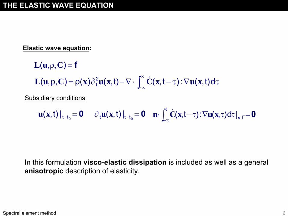
Elastic wave equation:
Subsidiary conditions:
f=),( CuL ρ,
THE ELASTIC WAVE EQUATION
In this
formulation
visco-elastic
dissipation
is
included
as well as a general anisotropic
description
of elasticity.
3Spectral element method
SPECTRAL-ELEMENT METHOD: General Concept
Subdivision of the
computational
domain
into
hexahedral
elements:
(a) 2D subdivision
that
honours
layer
boundaries
(b) Subdivision of the
globe
(cubed
sphere) (c) Subdivision with
topography
4Spectral element method
SPECTRAL-ELEMENT METHOD: General Concept
Mapping
to the
unit
cube:
5Spectral element method
SPECTRAL-ELEMENT METHOD: General Concept
Choice
of the
collocation
points:
Interpolation of Runge‘s
function
R(x)
using
6th-order
polynomials
and equidistant
collocation
points
211)(ax
xR+
=
interpolant
Runge‘s
phenomenon
6Spectral element method
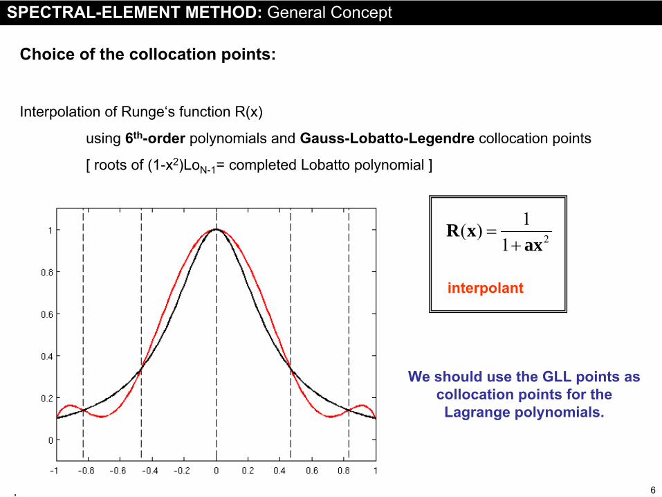
SPECTRAL-ELEMENT METHOD: General Concept
Choice
of the
collocation
points:
Interpolation of Runge‘s
function
R(x)
using
6th-order
polynomials
and Gauss-Lobatto-Legendre
collocation
points
[ roots
of (1-x2)LoN-1
= completed
Lobatto
polynomial
]
211)(ax
xR+
=
interpolant
We
should
use
the
GLL points
as collocation
points
for
the Lagrange
polynomials.
7Spectral element method
SPECTRAL-ELEMENT METHOD: General Concept
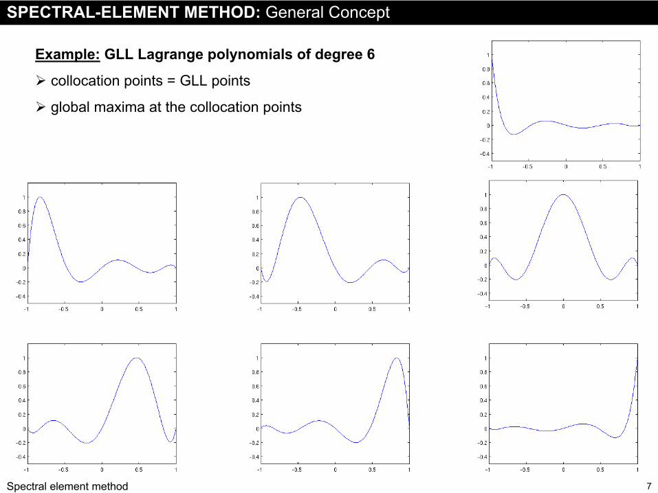
Example:
GLL Lagrange
polynomials
of degree
6
collocation points = GLL points
global maxima at the collocation points
8Spectral element method
The
SE system
Diagonal mass matrix
M
9Spectral element method
SPECTRAL-ELEMENT METHOD: General Concept
Numerical
quadrature
to determine
mass
and stiffness
matrices:
Quadrature
node
points
= GLL points
→ The
mass
matrix
is
diagonal, i.e., trivial to invert.
→ This
is
THE advantage
of the
spectral-element
method.
Time extrapolation:
2
)()(2)()(t
ttututtutuΔ
Δ−+−Δ+≈&&
[ ])()()()(2)( 12 tKutfMtttututtu −Δ+Δ−−=Δ+ −
10Spectral element method
SPECTRAL-ELEMENT METHOD: General Concept
Representation
in terms
of polynomials:
∑=
≈N
i
Nii xtutxu
0
)( )()(),( l
:)()( xNil Nth-degree
Lagrange
polynomials
→ We
can
transform
the
partial differential equation
into
an ordinary
differential equation
where
we
solve
for
the
polynomial
coefficients:
(within
the
unit
interval
[-1 1])
kikiiki fuKuM =−&&
::
ki
ki
KM mass
matrix
stiffness
matrix
11Spectral element method
SES3D: General Concept
Simulation of elastic wave propagation in a spherical section.
Spectral-element discretisation.
Computation of Fréchet kernels using the adjoint method.
Operates in natural spherical coordinates!
3D heterogeneous, radially anisotropic, visco-elastic.
PML as absorbing boundaries.
Programme philosophy:
Puritanism [easy to modify and
adapt to different problems, easy
implementation of 3D models,
simple code]
12Spectral element method
SES3D: Example
Southern Greece
8 June, 2008
Mw
=6.3
1.
Input files
[geometric
setup, source, receivers, Earth model]
2.
Forward simulation
[wavefield
snapshots
and seismograms]
3.
Adjoint
simulation
[adjoint
source, Fréchet
kernels]
13Spectral element method
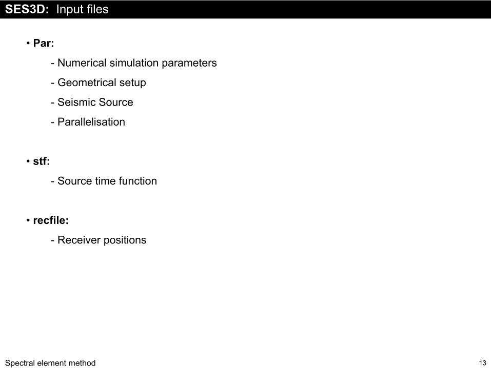
SES3D: Input files
• Par:
- Numerical
simulation
parameters
- Geometrical
setup
- Seismic
Source
- Parallelisation
• stf:
- Source
time function
• recfile:
-
Receiver positions
14Spectral element method
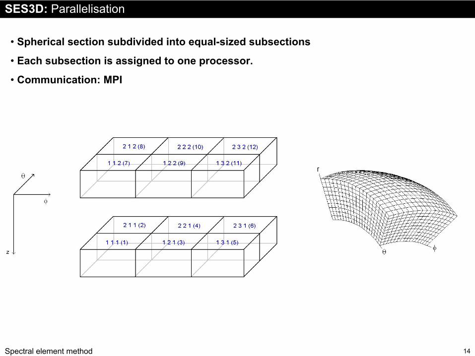
SES3D: Parallelisation
• Spherical
section
subdivided
into
equal-sized
subsections
• Each
subsection
is
assigned
to one
processor.
• Communication: MPI
15Spectral element method
SES3D: Source
time function
Source
time function
-
time step
and length
agree
with
the
simulation
parameters
-
PMLs
work
best with
bandpass
filtered
source
time functions
-
Example: bandpass
[50 s to 200 s]
16Spectral element method
Simulating
delta
functions?
17Spectral element method
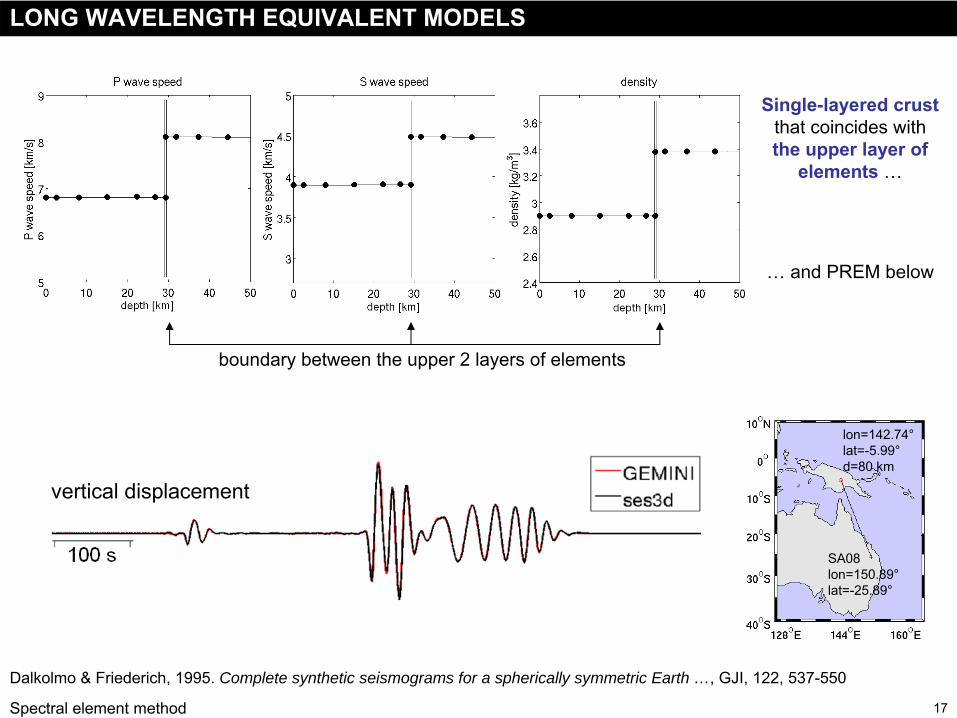
LONG WAVELENGTH EQUIVALENT MODELS
Single-layered
crust
that
coincides
with
the
upper
layer
of elements
…
… and PREM below
boundary
between
the
upper
2 layers
of elements
lon=142.74°lat=-5.99°d=80 km
SA08lon=150.89°lat=-25.89°
vertical
displacement
Dalkolmo
& Friederich, 1995. Complete synthetic seismograms for a spherically symmetric Earth …, GJI, 122, 537-550
18Spectral element method
2-layered crust
that
does
not
coincide
with
a layer
of elements
…
… and PREM below
boundary
between
the
upper
2 layers
of elements
lon=142.74°lat=-5.99°d=80 km
SA08lon=150.89°lat=-25.89°
verification
vertical
displacement
Dalkolmo
& Friederich, 1995. Complete synthetic seismograms for a spherically symmetric Earth …, GJI, 122, 537-550
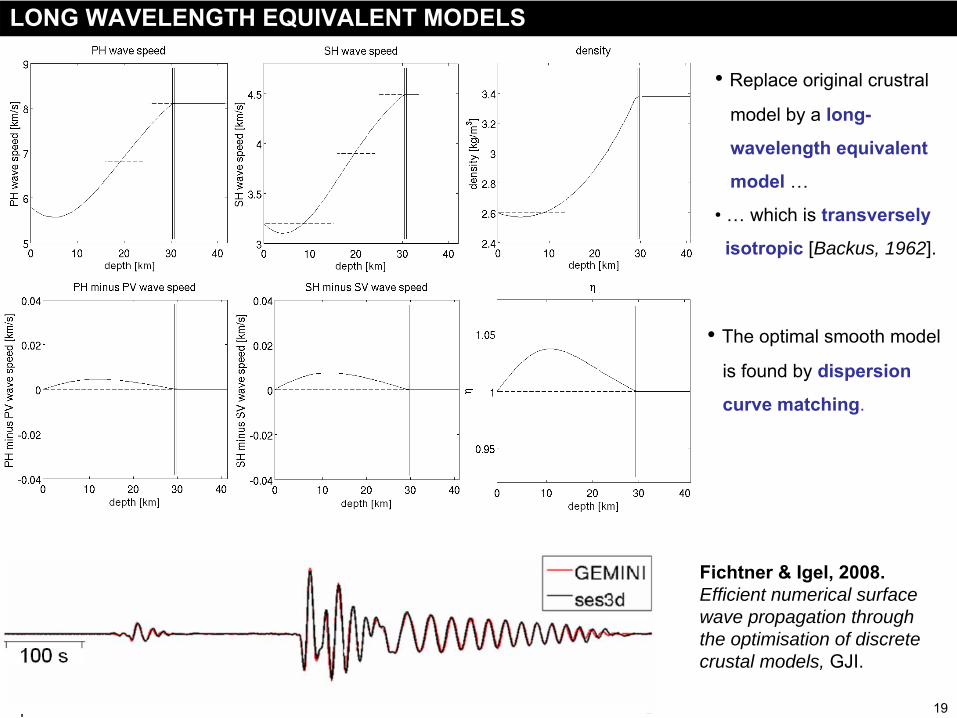
LONG WAVELENGTH EQUIVALENT MODELS
19Spectral element method
• Replace
original crustral
model
by
a long-
wavelength
equivalent
model
…
• … which is transversely
isotropic
[Backus, 1962].
• The
optimal smooth
model
is
found
by
dispersion
curve
matching.
Fichtner & Igel, 2008. Efficient numerical surface wave propagation through the optimisation of discrete crustal models, GJI.
long
wavelength
equivalent
modelsLONG WAVELENGTH EQUIVALENT MODELS
20Spectral element method
Minimisation
of the
phase
velocity
differences
for
the
fundamental and higher
modes
in the
frequency
range
of interest
through
simulated
annealing.
long
wavelength
equivalent
modelsLONG WAVELENGTH EQUIVALENT MODELS
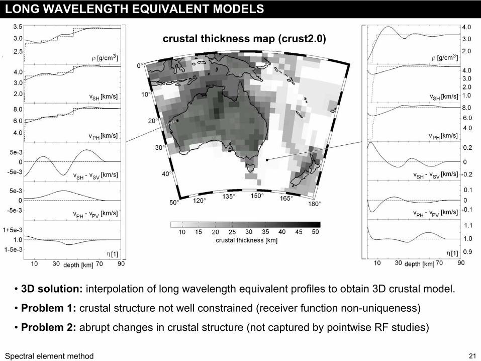
21Spectral element method
crustal
thickness
map
(crust2.0)
• 3D solution: interpolation
of long
wavelength
equivalent
profiles
to obtain
3D crustal
model.
• Problem 1: crustal
structure
not
well constrained
(receiver
function
non-uniqueness)
• Problem 2: abrupt changes
in crustal
structure
(not
captured
by
pointwise
RF studies)
long
wavelength
equivalent
modelsLONG WAVELENGTH EQUIVALENT MODELS
22Spectral element method
SES3D: Calls
to caution!
1.
Long-term
instability
of PMLs
-
All PML variants
are
long-term
unstable!
-
SES3D monitors
the
total kinetic
energy
Etotal
.
-
When
Etotal
increases
quickly, the
PMLs
are
switched
off and …
-
… absorbing
boundaries
are
replaced
by
less
efficient
multiplication
by
small
numbers.
2.
The
poles
and the
core
-
Elements become
infinitesimally
small
at the
poles
and the
core.
-
SES3D is
efficient
only
when
the
computational
domain
is
sufficiently
far from
the
poles
and the
core.
3.
Seismic
discontinuities
and the
crust
-
SEM is
very
accurate
only
when
discontinuities
coincide
with
element
boundaries.
-
SES3D‘s static
grid
may
not
always
achieve
this.
-
It
is
up to the
user
to assess
the
numerical
accuracy
in cases
where
discontinuities
run
through
elements. [Implement
long-wavelength
equivalent
models.]
-
Generally
no problem
for
the
410 km and 660 km discontinuities.
23Spectral element method
Spectral elements: summary
Spectral elements (SE) are a special form of the finite element method.The key difference is the choice of the basis (form) functions inside the elements, with which the fields are described. It is the Lagrange polynomials with Gauss-Lobato-Legendre (GLL) collocation points that make the mass matrix diagonal This leads to a fully explicit scheme without the need to perform a (sparse) matrix inverse inversionMaterial parameters can vary at each point inside the elementsSE works primarily on hexahedral gridsThe hexahedra can be curvilinear and adapt to complex geometries(cubed sphere, reservoir models)
Two open-source codes are available here: www.geodynamics.org (specfem3d) – regional and global scalewww.geophysik.uni-muenchen.de/Members/fichtner (ses3d) - regional scale