44
Speech Processing and Understanding CSC401 Assignment 3 1

Speech Processing and Understanding
CSC401 Assignment 3
1
2
Agenda
• Background
• Speech technology, in general
• Acoustic phonetics
• Assignment 3
• Speaker Recognition: Gaussian mixture models
• Speech Recognition: Word-error rates with Levenshtein
distance.

3
Applications of Speech Technology
Put this
there.
Multimodality & HCI
DictationMy hands are
in the air.Telephony
Emerging...
• Data mining/indexing.
• Assistive technology.
• Conversation.
Buy ticket...
AC490...
yes

4
Formants in sonorants
• However, formants are insufficient features for use in speech recognition generally...

5
Mel-frequency cepstral coefficients
• In real speech data, the
spectrogram is often transformed to a representation that more
closely represents human auditory
response and is more amenable to accurate classification.
• MFCCs are ‘spectra of spectra’. They are the discrete cosine
transform of the logarithms of the nonlinearly Mel-scaled powers of
the Fourier transform of windows
of the original waveform.

6
Challenges in speech data
• Co-articulation and dropped phonemes.
• (Intra-and-Inter-) Speaker variability.
• No word boundaries.
• Slurring, disfluency (e.g., ‘um’).
• Signal Noise.
• Highly dimensional.

7
Phonemes• Words are formed by phonemes (aka ‘phones’),
e.g., ‘pod’ = /p aa d/
• Words have different pronunciations. and in practice we can never be
certain of which phones were uttered, nor their start/stop points.
Syntactic
Lexical
Phonemic

8
Phonetic alphabets
• International Phonetic Association (IPA)
• Can represent sounds in all languages
• Contains non-ASCII characters
• ARPAbet
• One of the earliest attempts at encoding English for early speech recognition.
• TIMIT/CMU
• Very popular among modern databases for speech
recognition.

9
Example phonetic alphabets
• The other consonants are
transcribed as you would expect
• i.e., p, b, m, t, d, n, k, g, s,
z, f, v, w, h

10
Agenda
• Background
• Speech technology, in general
• Acoustic phonetics
• Assignment 3
• Speaker Recognition: Gaussian mixture models
• Speech Recognition: Word-error rates with Levenshtein
distance.
11
Assignment 3
• Two parts:
• Speaker identification: Determine which of 30 speakers an unknown test sample of speech comes from, given Gaussian
mixture models you will train for each speaker.
• Speech recognition: Compute word-error rates for speech recognition systems using Levenshtein distance.

12
Speaker Data
• 32 speakers (e.g., S-3C, S-5A).
• Each speaker has up to 12 training utterances.
• e.g., /u/csc401/A3/data/S-3C/0.wav
• Each utterance has 3 files:
• *.wav : The original wave file.
• *.mfcc.npy : The MFCC features in NumPy format
• *.txt : Sentence-level transcription.

13
Speaker Data (cont.)
• All you need to know: A speech utterance is an Nxd matrix
• Each row represents the features of a d-dimensional point in time.
• There are N rows in a sequence of N frames.
• The data is in numpy arrays *.mfcc.npy
• To read the files: np.load(‘1.mfcc.npy’)
N
1
2
1 2 ddata dimension
fram
es
tim
e

14
Speaker Data (cont.)
• You are given human transcriptions in transcripts.txt
• You are also given Kaldi and Google transcriptions in transcripts.*.txt.
• Ignore any symbols that are not words.

15
Agenda
• Background
• Speech technology, in general
• Acoustic phonetics
• Assignment 3
• Speaker Recognition: Gaussian mixture models
• Speech Recognition: Word-error rates with Levenshtein
distance.

16
Speaker Recognition
• The data is randomly split into training and testing utterances. We
don’t know which speaker produced which test utterance.
• Every speaker occupies a characteristic part of the acoustic space.
• We want to learn a probability distribution for each speaker that
describes their acoustic behaviour.
• Use those distributions to identify the speaker-dependent features of
some unknown sample of speech data.

17
Some background: fitting to data• Given a set of observations X of some random variable, we wish to
know how X was generated.
• Here, we assume that the data was sampled from a Gaussian
Distribution (validated by data).
• Given a new data point (x=15), It is more likely that x was generated by B.
A B
15 15

18
Finding parameters: 1D Gaussians
• Often called Normal distributions
• The parameters we can adjust to fit the data are and :

19
Maximum likelihood estimation
• Given data:
• and Parameter set:
• Maximum likelihood attempts to find the parameter set that
maximizes the likelihood of the data.
• The likelihood function provides a surface over all possible parameterizations. In order to find the Maximum
Likelihood, we set the derivative to zero:

20
MLE - 1D Gaussian
• Estimate :
• A similar approach gives the MLE estimate of :
21
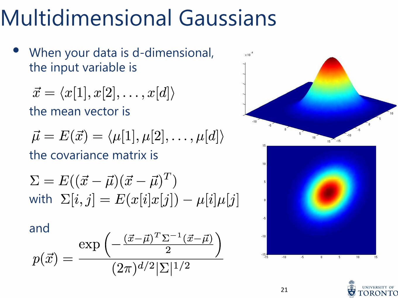
Multidimensional Gaussians
• When your data is d-dimensional,
the input variable is
the mean vector is
the covariance matrix is
with
and

22
Non-Gaussian data
• Our speaker data does not behave unimodally.
• i.e., we can't use just 1 Gaussian per speaker.
• E.g., observations below occur mostly bimodally, so fitting 1
Gaussian would not be representative.

23
Gaussian mixtures
• Gaussian mixtures are a weighted
linear combination of M component gaussians.

• For notational convenience,
• So
• To find , we solve where
24
MLE for Gaussian mixtures
...see Appendix for more

25
MLE for Gaussian mixtures (pt. 2)
• Given
• Since
• We obtain by solving for in :
and:

26
Recipe for GMM ML estimation
• Do the following for each speaker individually. Use all the frames
available in their respective Training directories
1. Initialize: Guess with M
random vectors in the data, or by performing M-means clustering.
2. Compute likelihood: Compute and
3. Update parameters:
Repeat 2&3 until converges

27
Cheat sheet
Probability of xt in the GMM
Probability of the mth
Gaussian, given xt
Probability of observing
xt in the mth Gaussian
Prior probability of the mth
Gaussian

28
Initializing theta
• Initialize each mum
to a random vector from the data.
• Initialize Sigmam
to a `random’ diagonal matrix (or identity matrix).
• Initialize omegam
randomly, with these constraints:
• A good choice would be to set omegam
to 1/M

29* Slide borrowed from Chris Bishop’s presentation
Solutions:• Ensure that the variances don’t get too small.• Bayesian GMMs
Your Task
• For each speaker, train a GMM, using the EM algorithm, assuming
diagonal covariance.
• Identify the speaker of each test utterance.
• Experiment with the number of mixture elements in the models,
the improvement threshold, number of possible speakers, etc.
• Comment on the results
30

Practical tips for MLE of GMMs
• We assume diagonal covariance matrices. This reduces the number
of parameters and can be sufficient in practice given enough components.
• Numerical Stability: Compute likelihoods in the log domain
(especially when calculating the likelihood of a sequence of frames).
• Here, and are d-dimensional vectors.
31

Practical tips (pt. 2)
• Efficiency: Pre-compute terms not dependent on
32

33
Agenda
• Background
• Speech technology, in general
• Acoustic phonetics
• Assignment 3
• Speaker Recognition: Gaussian mixture models
• Speech Recognition: Word-error rates with Levenshtein
distance.
34
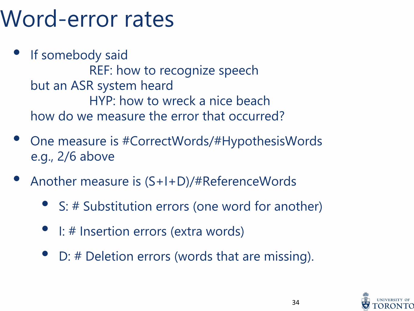
Word-error rates
• If somebody said
REF: how to recognize speech but an ASR system heard
HYP: how to wreck a nice beach
how do we measure the error that occurred?
• One measure is #CorrectWords/#HypothesisWords
e.g., 2/6 above
• Another measure is (S+I+D)/#ReferenceWords
• S: # Substitution errors (one word for another)
• I: # Insertion errors (extra words)
• D: # Deletion errors (words that are missing).

35
Computing Levenshtein Distance
• In the example
REF: how to recognize speech. HYP: how to wreck a nice beach
How do we count each of S, I, and D?
• If “wreck” is a substitution error, what about “a” and “nice”?

36
Computing Levenshtein Distance• In the example
REF: how to recognize speech.
HYP: how to wreck a nice beach
How do we count each of S, I, and D?
If “wreck” is a substitution error, what about “a” and “nice”?
• Levenshtein distance:
Initialize R[0,0] = 0, and R[i,j] = ∞ for all i=0 or j=0
for i=1..n (#ReferenceWords)
for j=1..m (#Hypothesis words)
R[i,j] = min(R[i-1,j] + 1 (deletion)
R[i-1,j-1] (only if words match)
R[i-1,j-1]+1 (only if words differ)
R[i,j-1] + 1 ) (insertion)
Return 100*R(n,m)/n

37
Levenshtein example

38
Levenshtein example

39
Levenshtein example

40
Levenshtein example
Word-error rate is 4/4 = 100%
2 substitutions, 2 insertions

41
Appendices

42
Multidimensional Gaussians, pt. 2
• If the ith and jth dimensions are statistically independent,
and
• If all dimensions are statistically independent, and
the covariance matrix becomes diagonal, which means
where

43
MLE example - dD Gaussians
• The MLE estimates for parameters given
i.i.d. training data are obtained by maximizing the joint likelihood
• To do so, we solve , where
• Giving
44
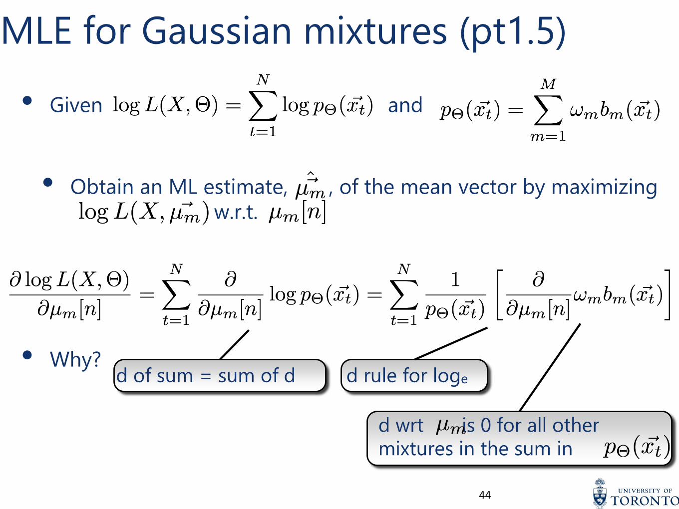
MLE for Gaussian mixtures (pt1.5)
• Given and
• Obtain an ML estimate, , of the mean vector by maximizing
w.r.t.
• Why?d of sum = sum of d d rule for loge
d wrt is 0 for all other
mixtures in the sum in


