Abstract Algorithm selection methods can be speeded-up substantially by incorporatingmulti-objective measures that give preference to algorithms that are both promising andfast to evaluate. In this paper, we introduce such a measure, A3R, and incorporate it intotwo algorithm selection techniques: average ranking and active testing. Average rankingcombines algorithm rankings observed on prior datasets to identify the best algorithms fora new dataset. The aim of the second method is to iteratively select algorithms to be testedon the new dataset, learning from each new evaluation to intelligently select the next bestcandidate. We show how both methods can be upgraded to incorporate a multi-objectivemeasure A3R that combines accuracy and runtime. It is necessary to establish the correctbalance between accuracy and runtime, as otherwise time will be wasted by conducting lessinformative tests. The correct balance can be set by an appropriate parameter setting withinfunction A3R that trades off accuracy and runtime. Our results demonstrate that the upgraded
versions of Average Ranking andActive Testing lead tomuch better mean interval loss valuesthan their accuracy-based counterparts.
Keywords Algorithm selection · Meta-learning · Ranking of algorithms · Average ranking ·Active testing · Loss curves · Mean interval loss
1 Introduction
A large number of data mining algorithms exist, rooted in the fields of machine learning,statistics, pattern recognition, artificial intelligence, and database systems, which are usedto perform different data analysis tasks on large volumes of data. The task to recommendthe most suitable algorithms has thus become rather challenging. Moreover, the problem isexacerbated by the fact that it is necessary to consider different combinations of parametersettings, or the constituents of composite methods such as ensembles.
The algorithm selection problem, originally described by Rice (1976), has attracted agreat deal of attention, as it endeavours to select and apply the best algorithm(s) for a giventask (Brazdil et al. 2008; Smith-Miles 2008). The algorithm selection problem can be castas a learning problem: the aim is to learn a model that captures the relationship between theproperties of the datasets, or meta-data, and the algorithms, in particular their performance.This model can then be used to predict the most suitable algorithm for a given new dataset.
This paper presents two new methods, which build on ranking approaches for algorithmselection (Brazdil and Soares 2000; Brazdil et al. 2003) in that it exploits meta-level infor-mation acquired in past experiments.
The first method is known as average ranking (AR), which calculates an average rankingfor all algorithms over all prior datasets. The upgrade here consists of using A3R, a multi-objective measure that combines accuracy and runtime (the time needed to evaluate a model).Many earlier approaches used only accuracy.
The secondmethod uses an algorithm selection strategy known as active testing (AT) (Leiteand Brazdil 2010; Leite et al. 2012). The aim of active testing is to iteratively select andevaluate a candidate algorithm whose performance will most likely exceed the performanceof previously tested algorithms. Here again, function A3R is used in the estimates of theperformance gain, instead of accuracy, as used in previous versions.
It is necessary to establish the correct balance between accuracy and runtime, as otherwisetime will be wasted by conducting less informative and slow tests. In this work, the correctbalance can be set by a parameter setting within the A3R function. We have identified asuitable value using empirical evaluation.
The experimental results are presented in the form of loss-time curves, where time isrepresented on a log scale. This representation is very useful for the evaluation of rankingsrepresenting schedules, as was shown earlier (Brazdil et al. 2003; van Rijn et al. 2015). Theresults presented in this paper show that the upgraded versions of AR and AT lead to muchbetter mean interval loss values (MIL) than their solely accuracy-based counterparts.
Our contributions are as follows.We introduce A3R, a measure that can be incorporated inmultiple meta-learning methods to boost the performance in loss-time space. We show howthis can be done with the AR and ATmethods and establish experimentally that performanceindeed increases drastically. As A3R requires one parameter to be set, we also experimentallyexplore the optimal value of this parameter.
123
Mach Learn (2018) 107:79–108 81
The remainder of this paper is organized as follows. In Sect. 2 we present an overview ofexisting work in related areas.
Section 3 describes the average ranking method with a focus on how it was upgradedto incorporate both accuracy and runtime. As the method includes a parameter, this sectiondescribes also howwe searched for the best setting. Finally, this section presents an empiricalevaluation of the new method.
Section 4 provides details about the active testing method. We explain how this methodrelates to the earlier proposals and how it was upgraded to incorporate both accuracy andruntime. This section includes also experimental results and a comparison of both upgradedmethods and their accuracy-based counterparts.
Section 5 is concerned with the issue of how robust the average rankingmethod is to omis-sions in themeta-dataset. This issue is relevant becausemeta-datasets gathered by researchersare very often incomplete. The final section presents conclusions and future work.
2 Related work
In this paper we are addressing a particular case of the algorithm selection problem (Rice1976), oriented towards the selection of classification algorithms. Various researchersaddressed this problem in the course of the last 25 years.
2.1 Meta-learning approaches to algorithm selection
One very common approach, that could now be considered as the classical approach, usesa set of measures to characterize datasets and establish their relationship to algorithm per-formance. This information is often referred to as meta-data and the dataset containing thisinformation as meta-dataset.
The meta-data typically includes a set of simple measures, statistical measures,information-theoretic measures and/or the performance of simple algorithms referred to aslandmarkers (Pfahringer et al. 2000; Brazdil et al. 2008; Smith-Miles 2008). The aim isto obtain a model that characterizes the relationship between the given meta-data and theperformance of algorithms evaluated on these datasets. This model can then be used to pre-dict the most suitable algorithm for a given new dataset, or alternatively, provide a rankingof algorithms, ordered by their suitability for the task at hand. Many studies conclude thatranking is in fact better, as it enables the user to iterative test the top candidates to identifythe algorithms most suitable in practice. This strategy is sometimes referred to as the Top-Nstrategy (Brazdil et al. 2008).
2.2 Active testing
The Top-N strategy has the disadvantage that it is unable to exploit the information acquiredin previous tests. For instance, if the top algorithm performs worse than expected, this maytell us something about the given dataset which can be exploited to update the ranking.Indeed, very similar algorithms are now also likely to perform worse than expected. This ledresearchers to investigate an alternative testing strategy, known as active testing (Leite et al.2012). This strategy intelligently selects the most useful tests using the concept of estimatesof performance gain.1 These estimates the relative probability that a particular algorithm
1 We prefer to use this term here, instead of the term relative landmarkers which was used in previouswork (Fürnkranz and Petrak 2001) in a slightly different way.
123
82 Mach Learn (2018) 107:79–108
will outperform the current best candidate. In this paper we attribute particular importanceto the tests on the new dataset. Our aim is to propose a way that minimizes the time beforethe best (or near best) algorithm is identified.
2.3 Active learning
Active Learning is briefly discussed here to eliminate a possible confusionwith active testing.The two concepts are quite different. Some authors have also used active learning for algo-rithm selection (Long et al. 2010), and exploited the notion of Expected Loss Optimization(ELO). Another notable active learning approach to meta-learning was presented by Prudên-cio and Ludermir (2007), where the authors used active learning to support the selection oninformative meta-examples (i.e. datasets). Active learning is somewhat related to experimentdesign (Fedorov 1972).
2.4 Combining accuracy and runtime
Different proposals were made in the past regarding how to combine accuracy and runtime.One early proposal involved function ARR (adjusted ratio of ratios) (Brazdil et al. 2003),which has the form:
ARRdiaref ,a j
=
SRdia j
SRdiaref
1 + AccD ∗ log(T dia j /T
diaref )
(1)
Here, SRdia j and SRdi
aref represent the success rates (accuracies) of algorithms a j and aref ondataset di , where aref represents a given reference algorithm. Instead of accuracy, AUC or
another measure can be used as well. Similarly, T dia j and T di
aref represent the run times of thealgorithms, in seconds.
AccD is a parameter that needs to be set and represents the amount of accuracy he/she iswilling to trade for a 10 times speed-up or slowdown. For example, AccD = 10% means thatthe user is willing to trade 10% of accuracy for 10 times speed-up/slowdown.
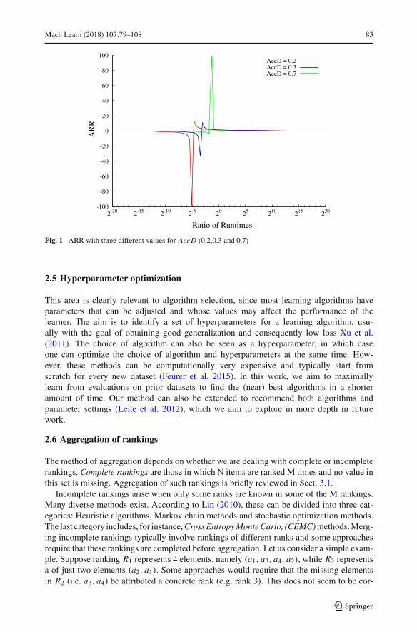
The ARR function should ideally be monotonically increasing. Higher success rate ratiosshould lead to higher values of ARR. Higher time ratios should lead to lower values of ARR.The overall effect of combining the two should again be monotonic. In one earlier work(Abdulrahman and Brazdil 2014) the authors have decided to verify whether this propertycan be verified on data. This study is briefly reproduced in the following paragraphs.
The value of SRR was fixed to 1 and the authors varied the time ratio from very smallvalues 2−20 to very high ones 220 and calculated the ARR for three different values of AccD(0.2, 0.3 and 0.7). The result can be seen in Fig. 1. The horizontal axis shows the log of thetime ratio (logRT ). The vertical axis shows the ARR value.
As can be seen, the resultingARR function is notmonotonic and even approaching infinityat some point. Obviously, this can lead to incorrect rankings provided by the meta-learner.
This problem could be avoided by imposing certain constraints on the values of the ratio,but herewe prefer to adopt a different function,A3R, that also combines accuracy and runtimeand exhibits a monotonic behaviour. It is described in Sect. 3.3.
123
Mach Learn (2018) 107:79–108 83
-100
-80
-60
-40
-20
0
20
40
60
80
100
2-20 2-15 2-10 2-5 20 25 210 215 220
AR
R
Ratio of Runtimes
AccD = 0.2AccD = 0.3AccD = 0.7
Fig. 1 ARR with three different values for AccD (0.2,0.3 and 0.7)
2.5 Hyperparameter optimization
This area is clearly relevant to algorithm selection, since most learning algorithms haveparameters that can be adjusted and whose values may affect the performance of thelearner. The aim is to identify a set of hyperparameters for a learning algorithm, usu-ally with the goal of obtaining good generalization and consequently low loss Xu et al.(2011). The choice of algorithm can also be seen as a hyperparameter, in which caseone can optimize the choice of algorithm and hyperparameters at the same time. How-ever, these methods can be computationally very expensive and typically start fromscratch for every new dataset (Feurer et al. 2015). In this work, we aim to maximallylearn from evaluations on prior datasets to find the (near) best algorithms in a shorteramount of time. Our method can also be extended to recommend both algorithms andparameter settings (Leite et al. 2012), which we aim to explore in more depth in futurework.
2.6 Aggregation of rankings
The method of aggregation depends on whether we are dealing with complete or incompleterankings. Complete rankings are those in which N items are ranked M times and no value inthis set is missing. Aggregation of such rankings is briefly reviewed in Sect. 3.1.
Incomplete rankings arise when only some ranks are known in some of the M rankings.Many diverse methods exist. According to Lin (2010), these can be divided into three cat-egories: Heuristic algorithms, Markov chain methods and stochastic optimization methods.The last category includes, for instance,CrossEntropyMonteCarlo, (CEMC)methods.Merg-ing incomplete rankings typically involve rankings of different ranks and some approachesrequire that these rankings are completed before aggregation. Let us consider a simple exam-ple. Suppose ranking R1 represents 4 elements, namely (a1, a3, a4, a2), while R2 representsa of just two elements (a2, a1). Some approaches would require that the missing elementsin R2 (i.e. a3, a4) be attributed a concrete rank (e.g. rank 3). This does not seem to be cor-
123
84 Mach Learn (2018) 107:79–108
rect: we should not be forced to assume that some information exists when in fact we havenone.2
In Sect. 5.1 we address the problem of robustness against incomplete rankings. This ariseswhenwe have incomplete test results in themeta-dataset.We have investigated howmuch theperformance of our methods degrades under such circumstances. Here we have developeda simple heuristic method based on Borda’s method reviewed in Lin (2010). In the studiesconducted by this author, simple methods often compete quite well with other more complexapproaches.
2.7 Multi-armed bandits
The multi-armed bandit problem involves a gambler whose aim is to decide which arm ofa K-slot machine to pull to maximize his total reward in a series of trials. Many real-worldlearning and optimization problems can be modeled in this way and algorithm selection isone of them. Different algorithms can be compared to different arms. Gathering knowledgeabout different arms can be compared to the process of gathering meta-data which involvesconducting testswith the given set of algorithms on given datasets. This phase is often referredto as exploration.
Manymeta-learning approaches assume that tests have beendone off-linewithout any cost,prior to determining which is the best algorithm for the new dataset. This phase exploits themeta-knowledge acquired and hence can be regarded as exploration. However, the distinctionbetween the two phases is sometimes not so easy to define. For instance, in the active testingapproach discussed in Sect. 4, tests are conducted both off-line and online, while the newdataset is being used. Previous tests condition which tests are done next.
Several strategies or algorithms have been proposed as a solution to themulti-armed banditproblem in the last twodecades. Some researchers have introduced so called contextual-banditproblem, where different arms are characterized by features. For example, some authors (Liet al. 2010) have applied this approach to personalized recommendation of news articles.In this approach a learning algorithm sequentially selects articles to serve users based oncontextual information about the users and articles, while simultaneously adapting its article-selection strategy based on user-click feedback. Contextual approaches can be compared tometa-learning approaches that exploit dataset features.
Many articles on multi-armed bandits are based on the notion of reward which is receivedafter an arm has been pulled. The difference to the optimal is often referred to as regret or loss.Typically, the aim is to maximize the accumulated reward, which is equivalent to minimizingthe accumulated loss, as different arms are pulled. Although initial studies were done on thisissue (e.g. Jankowski (2013)), this area has, so far, been rather under-explored. To the best ofour knowledge there is no work that would provide an algorithmic solution to the problemof which arm to pull when pulling different arms can take different amounts of time. So onenovelty of this paper is that it takes the time of tests into account with an adequate solution.
3 Upgrading the average ranking method by incorporating runtime
The aim of this paper is to determine whether the following hypotheses can be accepted:
2 We have considered using a package of R RankAggreg (Pihur et al. 2009), but unfortunately we would haveto attribute a concrete rank (e.g. k+1) to all missing elements.
123
Mach Learn (2018) 107:79–108 85
Hyp1: The incorporation of a function that combines accuracy and runtime is useful for theconstruction of the average ranking, as it leads to better results than just accuracywhen carrying out evaluation on loss-time curves.
Hyp2: The incorporation of a function that combines accuracy and runtime for the activetesting method leads to better results than only using accuracy when carrying outevaluation on loss-time curves.
The rest of this section is dedicated to the average ranking method. First, we present abrief overview of the method and show how the average ranking can be constructed onthe basis of prior test results. This is followed by the description of the function A3R thatcombines accuracy and runtime, and how the average ranking method can be upgraded withthis function. Furthermore, we empirically evaluate this method by comparing the rankingobtained with the ranking representing the golden standard. Here we also introduce loss-timecurves, a novel representation that is useful in comparisons of rankings.
As our A3R function includes a parameter that determines the weight attributed to eitheraccuracy or time, we have studied the effects of varying this parameter on the overall perfor-mance. As a result of this study, we identify the range of values that led to the best results.
3.1 Overview of the average ranking method
This section presents a brief review of the average ranking method that is often used incomparative studies in the machine learning literature. This method can be regarded as avariant of Borda’s method (Lin 2010).
For each dataset, the algorithms are ordered according to the performancemeasure chosen(e.g., predictive accuracy) and ranks are assigned accordingly. Among many popular rankingcriteria we find, for instance, success rates, AUC, and significant wins (Brazdil et al. 2003;Demšar 2006; Leite and Brazdil 2010). The best algorithm is assigned rank 1, the runner-upis assigned rank 2, and so on. Should two or more algorithms achieve the same performance,the attribution of ranks is done in two steps. In the first step, the algorithms that are tied areattributed successive ranks (e.g. ranks 3 and 4). Then all tied algorithms are assigned themean rank of the occupied positions (i.e. 3.5).
Let r ji be the rankof algorithm i ondataset j . In thisworkweuseaverage ranks, inspired by
Friedman’sM statistic (Neave and Worthington 1988). The average rank for each algorithmis obtained using
ri =⎛⎝
D∑j=1
r ji
⎞⎠ ÷ D (2)
where D is the number of datasets. The final ranking is obtained by ordering the averageranks and assigning ranks to the individual algorithms accordingly.
The average ranking represents a quite useful method for decidingwhich algorithm shouldbe used. Also, it can be used as a baseline against which other methods can be compared.
The average ranking would normally be followed on the new dataset: first the algorithmwith rank 1 is evaluated, then the one with rank 2 and so on. In this context, the averageranking can be referred to as the recommended ranking.
3.1.1 Evaluation of rankings
The quality of a ranking is typically established through comparisonwith the golden standard,that is, the ideal ranking on the new (test) dataset(s). This is often done using a leave-one-out
123
86 Mach Learn (2018) 107:79–108
0
0.2
0.4
0.6
0.8
1
0 2 4 6 8 10 12 14 16 18 20
Acc
urac
y Lo
ss %
Number of Tests
0
0.2
0.4
0.6
0.8
1
0 1000 2000 3000 4000 5000 6000
Acc
urac
y Lo
ss %
Time
0
0.2
0.4
0.6
0.8
1
0.5 1 1.5 2 2.5 3 3.5 4
Acc
urac
y Lo
ss %
Log of Time(a) (b) (c)
Fig. 2 Loss curves for accuracy-based average ranking. a Loss-curve. b Loss-time Curve. c Loss-time curve(log)
cross-validation (CV) strategy (or in general k-fold CV) on all datasets: in each leave-one-outcycle the recommended ranking is compared against the ideal ranking on the left-out dataset,and then the results are averaged for all cycles.
Different evaluationmeasures can be used to evaluate how close the recommended rankingis to the ideal one. Often, this is a type of correlation coefficient. Here we have opted forSpearman’s rank correlation (Neave and Worthington 1988), but Kendall’s Tau correlationcould have been used aswell. Obviously, wewant to obtain rankings that are highly correlatedwith the ideal ranking.
A disadvantage of this approach is that it does not show directly what the user is gainingor losing when following the ranking. As such, many researchers have adopted a secondapproach which simulates the sequential evaluation of algorithms on the new dataset (usingcross-validation) as we go down the ranking. The measure that is used is the performanceloss, defined as the difference in accuracy between abest and a∗, where abest represents thebest algorithm identified by the system at a particular time and a∗ the truly best algorithmthat is known to us (Leite et al. 2012).
As tests proceed following the ranking, the loss either maintains its value, or decreaseswhen the newly selected algorithm improved upon the previously selected algorithms, yield-ing a loss curve. Many typical loss curves used in the literature show how the loss dependson the number of tests carried out. An example of such curve is shown in Fig. 2a. Evaluationis again carried out in a leave-one-out fashion. In each cycle of the leave-one-out cross-validation (LOO-CV) one loss curve is generated. In order to obtain an overall picture, theindividual loss-time curves are aggregated into a mean loss curve. An alternative to usingLOO-CV would be to use k-fold CV (with e.g. k=10). This issue is briefly discussed inSect. 6.1.
3.1.2 Loss-time curves
A disadvantage of loss curves it that they only show how loss depends on the number of tests.However, some algorithms are much slower learners than others—sometimes by severalorders of magnitude, and these simple loss curves do not capture this.
This is why, in this article, we follow Brazdil et al. (2003) and van Rijn et al. (2015) andtake into account the actual time required to evaluate each algorithm and use this informationwhen generating the loss curve. We refer to this type of curve as a loss versus time curve, orloss-time curve for short. Figure 2b shows an example of a loss-time curve, correspondingto the loss curve in Fig. 2a.
As train/test times include both very small and very large numbers, it is natural to use thelogarithm of the time (log10), instead of the actual time. This has the effect that the same time
123
Mach Learn (2018) 107:79–108 87
intervals appear to be shorter as we shift further on along the time axis. As normally the userwould not carry out exhaustive testing, but rather focus on the first few items in the ranking,this representation makes the losses at the beginning of the curve more apparent. Figure 2cshows the arrangement of the previous loss-time curve on a log scale.
Each loss time curve can be characterized by a number representing the mean loss ina given interval, an area under the loss-time curve. The individual loss-time curves can beaggregated into a mean loss-time curve. We want this mean interval loss (MIL) to be as lowas possible. This characteristic is similar to AUC, but there is one important difference.Whentalking about AUCs, the x-axis values spans between 0 and 1, while our loss-time curves spanbetween some Tmin and Tmax defined by the user. Typically the user searching for a suitablealgorithm would not worry about very short times where the loss could still be rather high.In the experiments here we have set Tmin to 10 s. In an on-line setting, however, we mightneed a much smaller value. The value of Tmax needs also to be set. In the experiments hereit has been set to 104 s corresponding to about 2.78h. We assume that most users would bewilling to wait a few hours, but not days, for the answer. Also, many of our loss curves reach0, or values very near 0 at this time. Note that this is an arbitrary setting that can be changed,but here it enables us to compare loss-time curves.
3.2 Data used in the experiments
This section describes the dataset used in the experiments described in this article. The meta-dataset was constructed from evaluation results retrieved from OpenML (Vanschoren et al.2014), a collaborative science platform for machine learning. This dataset contains the resultsof 53 parameterized classification algorithms from theWeka workbench (Hall et al. 2009) on39 classification datasets.3 More details about the 53 classification algorithms can be foundin the Appendix.
3.3 Combining accuracy and runtime
In many situations, we have a preference for algorithms that are fast and also achieve highaccuracy. However, the question is whether such a preference would lead to better loss-timecurves. To investigate this, we have adopted a multi-objective evaluation measure, A3R,described in Abdulrahman and Brazdil (2014), that combines both accuracy and runtime.Here we use a slightly different formulation to describe this measure:
A3Rdiaref ,a j
=
SRdia j
SRdiaref
(T dia j /T
diaref )
P(3)
Here SRdia j and SRdi
aref represent the success rates (accuracies) of algorithms a j and aref ondataset di , where aref represents a given reference algorithm. Instead of accuracy, AUC or
another measure can be used as well. Similarly, T dia j and T di
aref represent the run times of thealgorithms, in seconds.
To trade off the importance of time, the denominator is raised to the power of P, whileP is usually some small number, such as 1/64, representing in effect, the 64th root. Thisis motivated by the observation that run times vary much more than accuracies. It is notuncommon that one particular algorithm is three orders of magnitude slower (or faster) than
Table 1 Effect of varying P ontime ratio C P = 1/2C 1000P C P = 1/2C 1000P
0 1 1000.000 6 1/64 1.114
1 1/2 31.623 7 1/128 1.055
2 1/4 5.623 8 1/256 1.027
3 1/8 2.371 9 1/512 1.013
4 1/16 1.539 10 1/1024 1.006
5 1/32 1.241 ∞ 0 1.000
another. Obviously, we do not want the time ratios to completely dominate the equation. Ifwe take the Nth root of the ratios, we will get a number that goes to 1 in the limit, when Nis approaching infinity (i.e. if P is approaching 0).
For instance, if we used P = 1/256, an algorithm that is 1000 times slower would yield adenominator of 1.027. It would thus be equivalent to the faster reference algorithm only if itsaccuracy was 2.7% higher than the reference algorithm. Table 1 shows how a ratio of 1000(one algorithm is 1000 times slower than the reference algorithm) is reduced for decreasingvalues of P . As P gets lower, the time is given less and less importance.
A simplified version of A3R introduced in van Rijn et al. (2015) assumes that both thesuccess rate of the reference algorithm SRdi
aref and the corresponding time T diaref have a fixed
value. Here the values are set to 1. The simplified version, A3R′, which can be shown toyield the same ranking, is defined as follows:
A3R′dia j
= SRdia j
(T dia j )
P(4)
We note that if P is set to 0, the value of the denominator will be 1. So in this case, onlyaccuracy will be taken into account. In the experiments described further on we used A3R(not A3R′).
3.3.1 Upgrading the average ranking method using A3R
The performance measure A3R can be used to rank a given set of algorithms on a particulardataset in a similar way as accuracy. Hence, the average rank method described earlier wasupgraded to generate a time-aware average ranking, referred to as the A3R-based averageranking.
Obviously, we can expect somewhat different results for each particular choice of param-eter P that determines the relative importance of accuracy and runtime, thus it is importantto determine which value of P will lead to the best results in loss-time space. Moreover, wewish to know whether the use of A3R (with the best setting for P) achieves better resultswhen compared to the approach that only uses accuracy. The answers to these issues areaddressed in the next sections.
3.3.2 Searching for the best parameter setting
Our first aim was to generate different variants of the A3R-based average ranking resultingfrom different settings of P within A3R and identify the best setting. We have used a gridsearch and considered settings of P ranging from P=1/4 until P=1/256, shown in Table 2.
123
Mach Learn (2018) 107:79–108 89
Table 2 Mean interval loss of AR-A3R associated with the loss-time curves for different values of P
P= 1/4 1/16 1/64 1/128 1/256 0
MIL 0.752 0.626 0.531 0.535 0.945 22.11
The bold value indicates the best value corresponding to the lowest MIL loss
0
0.2
0.4
0.6
0.8
1
1.2
1.4
1.6
1.8
2
1e+0 1e+1 1e+2 1e+3 1e+4 1e+5 1e+6
Acc
urac
y Lo
ss (%
)
Time (seconds)
AR-A3R-1/4AR*AR0
Fig. 3 Loss-time curves for A3R-based and accuracy-based average ranking
The last value shown is P=0. If this value is used in (T dia j /T
diaref )
P the result would be 1. Thelast option corresponds to a variant when only accuracy matters.
All comparisons were made in terms of mean interval loss (MIL) associated with themean loss-time curves. As we have explained earlier, different loss-time curves obtained indifferent cycles of leave-one-out method are aggregated into a single mean loss-time curve,shown also in Fig. 3. For each one we calculated MIL, resulting in Table 2.
TheMIL values in this table representmean values for different cycles of the leave-one-outmode. In each cycle the method is applied to one particular dataset.
The results show that the setting of P=1/64 leads to better results than other values, whilethe setting P=1/128 is not too far off. Both settings are better than, for instance, P=1/4, whichattributes a much higher importance to time. They are also better than, for instance, P=1/256which attributes much less importance to time, or to P=0 when only accuracy matters.
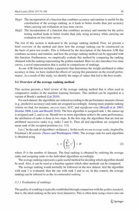
The boxplots in Fig. 4 show how the MIL values vary for different datasets. The boxplotsare in agreement with the values shown in Table 2. The variations are lowest for the settingsP=1/16, P=1/64 and P=1/128, although for each onewe note various outliers. The variationsare much higher for all the other settings. The worst case is P=0 when only accuracy matters.
For simplicity, the best version identified, that is AR-A3R-1/64, is identified by the shortname AR* in the rest of this article. Similarly, the version AR-A3R-0 corresponding to thecase when only accuracy matters is referred to as AR0.
AsAR*produces better results thanAR0we have provided evidence in favor of hypothesisHyp1 presented earlier.
An interesting question arises why AR0 has such a bad performance. Using AR withaccuracy-based ranking leads to disastrous results (MIL=22.11) and should be avoided atall costs! This issue is addressed further on in Sect. 5.2.2.
123
90 Mach Learn (2018) 107:79–108
Fig. 4 Boxplots showing thedistribution of MIL values for thesettings of P
1/4 1/16 1/64 1/128 1/256 00
24
68
AR−A3R variants
MIL
val
ues
3.3.3 Discussion
Parameter P could be used as a user-defined parameter to determine his/her relative intereston accuracy or time. In other words, this parameter could be used to establish the trade-offbetween accuracy and runtime, depending on the operation condition required by the user(e.g. a particular value of Tmax , determining the time budget).
However, one very important result of our work is that there is an optimum for which theuser will obtain the best result in terms of MIL.
The values of Tmin and Tmax define an interval of interest in which we wish to minimizeMIL. It is assumed that all times in this interval are equally important. We assume that theuser could interrupt the process at any time T lying in this interval and request the name ofabest , the best algorithm identified.
4 Active testing using accuracy and runtime
Themethod of A3R-based average ranking described in the previous section has an importantshortcoming: if the given set of algorithms includes many similar variants, these will be closeto each other in the ranking, and hence their performancewill be similar on the new dataset. Inthese circumstances it would be beneficial to try to use other algorithms that could hopefullyyield better results. The AR method, however, passively follows the ranking, and hence isunable to skip very similar algorithms.
This problem is quite common, as similar variants can arise for many reasons. One reasonis that many machine learning algorithms include various parameters which may be set todifferent values, yet have limited impact. Even if we used a grid of values and selected onlysome of possible alternative settings, we would end up with a large number of variants. Manyof them will exhibit rather similar performance.
Clearly, it is desirable to have a more intelligent way to choose algorithms from theranking. One very successful way to do this is active testing (Leite et al. 2012). This methodstarts with a current best algorithm, abest , which is initialized to the topmost algorithm in theaverage ranking. It then selects new algorithms in an iterative fashion, searching in each step
123
Mach Learn (2018) 107:79–108 91
for the best competitor, ac. This best competitor is identified by calculating the estimatedperformance gain of each untested algorithmwith respect to abest and selecting the algorithmthatmaximizes this value. In Leite et al. (2012) the performance gainwas estimated by findingthe most similar datasets, looking up the performance of every algorithm, and comparing thatto the performance of abest on those datasets. If another algorithm outperforms abest onmanysimilar datasets, it is a good competitor.
In this paper we have decided to use a simpler approach without focusing on the mostsimilar datasets, but correct one major shortcoming, which is that it does not take runtimeinto account. As a result, this method can spend a lot of time evaluating slow algorithms evenif they are expected to be even marginally better. Hence, our aim is to upgrade the activetesting method by incorporating A3R as the performance measure and analyzing the benefitsof this change. Moreover, as A3R includes a parameter P, it is necessary to determine thebest value for this setting.
4.1 Upgrading active testing with A3R
In this section we describe the upgraded active testing method in more detail. The main algo-rithm is presented inAlgorithm 1 (AT-A3R), which shows how the datasets are used in a leave-one-out evaluation. In step 5 themethod constructs the AR∗ average ranking, A. This rankingis used to identify the topmost algorithm, which is used to initialize the value of abest . ThenAlgorithm 2 (AT -A3R′) containing the actual active testing procedure is invoked. Itsmain aimis to construct the loss curve Li for one particular dataset di and add it to the other loss curvesLs. The final step involves aggregating all loss curves and returning themean loss curve Lm .
Algorithm 1 AT-A3R - Active testing with A3RRequire: algorithms A, datasets Ds, parameter P1: Ls ← () (Initialize the list of loss-time curves to an empty list)2: Leave-one-out cycle (di represents dnew):3: for all di in Ds do4: Dx ← Ds − di5: Construct AR∗ average ranking, A, of algorithms A on Dx6: abest ← A[1] (the topmost element)7: A ← A − abest8: (Li , abest) ← ATA3R’(di,Dx, abest , A,P) (Algorithm 2)9: Add the new loss curve Li to the list:
Ls ← Ls +++ Li10: end for11: Construct the mean loss curve Lm by aggregating all loss cuves in LsReturn: Mean loss curve Lm
4.1.1 Active testing with A3R on one dataset
The main active testing method in Algorithm 2 includes several steps:Step 1: It is used to initialize certain variables.Step 2: The performance of the current best algorithm abest on dnew is obtained using a
cross-validation (CV) test.Steps 3–12 (overview): These steps include awhile loop, which at each iteration identifies
the best competitor (step 4), removes it from the ranking A (step 5) and obtains its performance(step 6). If its performance exceeds the performance of abest , it replaces it. This process isrepeated until all algorithms have been processed. More details about the individual steps aregiven in the following paragraphs.
123
92 Mach Learn (2018) 107:79–108
Algorithm 2 ATA3R’ - Active testing with A3R on one dataset
Require: di , Dx , abest , A, P1: Initialize ranking dnew and loss curve Li :
dnew ← di, Li ← ()
2: Obtain the performance of abest on dataset dnew using a CV test:
(Tdnewabest , SRdnewabest ) ← CV (abest , dnew)
3: while | A| > 0 do4: Find the most promising competitor ac of abest using estimates of performance gain:
ac = argmaxak
∑di∈Ds ΔPf (ak , abest , di )
5: A ← A−−− ac (Remove ac from A)6: Obtain the performance of ac on dataset dnew using a CV test:
(Tdnewac , SRdnewac ) ← CV (ac, dnew)
Li ← Li + (Tdnewac , SRdnewac )
7: Compare the accuracy performance of ac with abest and carry out updates:
8: if SRdnewac > SRdnewabest then
9: abest ← ac, Tdnewabest ← Tdnew
ac , SRdnewabest ← SRdnewac10: end if11: end while12: return Loss-time curve Li and abest
Step 4: This step is used to identify the best competitor. This is done by considering allpast tests and calculating the sum of estimated performance gains ΔPf for different datasets.This is repeated for all different algorithms and the one with the maximum sum of ΔPf isused as the best competitor ac, as shown in Eq. 5:
ac = argmaxak
∑di∈D
ΔPf (ak, abest , di ) (5)
The estimate of performance gain, ΔPf , is reformulated in terms of A3R:
ΔPf (aj, abest , di ) = r
⎛⎜⎜⎜⎜⎝
SRdia j
SRdiabest
(T dia j /T
diabest )
P− 1 > 0
⎞⎟⎟⎟⎟⎠
∗
⎛⎜⎜⎜⎜⎝
SRdia j
SRdiabest
(T dia j /T
diabest )
P− 1
⎞⎟⎟⎟⎟⎠
(6)
where a j is an algorithm and di a dataset. The function r(test) returns 1 if the test is trueand 0 otherwise.
An illustrative example is presented in Fig. 5, showing different values of ΔPf of onepotential competitor with respect to abest on all datasets.
Table 3 shows the estimates of potential performance gains for 5 potential competitors.The competitor with the highest value (a2) is chosen, expecting that it will improve theaccuracy on the new dataset.
Step 6: After the best competitor has been identified, the method proceeds with a cross-validation (CV) test on the newdataset to obtain the actual performance of the best competitor.After this the loss curve Li is updated with the new information.
Step 7-10: A test is carried to determine whether the best competitor is indeed better thanthe current best algorithm. If it is, the new competitor is used as the new best algorithm.
Fig. 5 Values of ΔPf of a potential competitor with respect to abest on all datasets
Table 3 Determining the bestcompetitor among differentalternatives
Algorithm∑
ΔPf
a1 0.587
a2 3.017
a3 0.143
a4 0.247
a5 1.280
The bold value indicates thehighest estimated performancegain
Table 4 MIL values of AT-A3R for different parameter setting of P
P 1 1/2 1/4 1/8 1/16 1/32 1/64 1/128 0
MIL 0.846 0.809 0.799 0.809 0.736 0.905 1.03 1.864 3.108
The bold value indicates the best value
Step 12: In this step the loss-time curve Li is returned together with the final best algorithmabest identified.
4.2 Optimizing the parameter settings for AT-A3R
To use AT-A3R in practice we need to determine a good setting of parameter P in A3R usedwithin AT-A3R.We have considered different values shown in Table 4. The last value shown,P=0, represents a situation when only accuracy matters.
The empirical results presented in this table indicate that the optimal parameter settingfor P is 1/16 for the datasets used in our experiments. We will refer to this variant of activetesting as AT-A3R-1/16, or AT* for simplicity. We note, however, that the MIL values do notvary much when the values of P are larger than 1/16 (i.e. 1/4 etc.). For all these setting timeis given a high importance.
When time is ignored, which corresponds to the setting of P=0 and the version is AT-A3R-0. For simplicity, this version will be referred to as AT0 in the rest of this article.
The MIL values in this table represent mean interval values obtained in different cyclesof the leave-one-out mode. Individual values vary quite a lot for different datasets, as can beseen in the boxplots in Fig. 6. The loss-time curves for some of the variants are shown inFig. 7.
This study has provided an evidence that the AT method too works quite well when timeis taken into consideration. When time is ignored (version AT0), the results are quite poor
123
94 Mach Learn (2018) 107:79–108
Fig. 6 Boxplot showing thedistribution of MIL values for themethods in Table 4
1/4 1/8 1/16 1/32 1/64 00
24
68
AT−A3R Variants
MIL
val
ues
0
0.2
0.4
0.6
0.8
1
1.2
1.4
1.6
1.8
2
1e+0 1e+1 1e+2 1e+3 1e+4 1e+5 1e+6 1e+7
Acc
urac
y Lo
ss (%
)
Time (seconds)
AT*AT-A3R-1/4
AT0
Fig. 7 Mean loss-time curves for AT-A3R with different settings for P
(MIL=3.108). But if we compare AT0 and AR0 approaches, the AT0 result is not so bad incomparison.
The fact that AT0 achieved much better value that AR0 can be explained by the initial-ization step used in Algorithm 1. We note that the AR* has been used to initialize the valueof abest . This version takes runtime into account. If AR0 were used instead, the MIL of AT0would increase to 21.89%, that is a value comparable to AR0.
The values shown in Table 4 and the accompanying boxplot indicate that the MIL scoresfor the AT method have relatively high variance. One plausible explanation for this is thefollowing. The method selects the best competitor on the basis of the estimate of the highestperformance gain. Here the topmost element is used in an ordered list. However, there maybe other choices with rather similar value, albeit a bit smaller, which are ignored. If theconditions are changed slightly, the order in the list changes and this affects the choice of thebest competitor and all subsequent steps.
123
Mach Learn (2018) 107:79–108 95
Table 5 MIL values of the AR and AT variants described above
Method AR* AT* AR0 AT0
MIL 0.531 0.736 22.11 3.108
The bold value indicates that the AR* method achieves the lowest loss
0
0.2
0.4
0.6
0.8
1
1.2
1.4
1.6
1.8
2
1e+0 1e+1 1e+2 1e+3 1e+4 1e+5 1e+6 1e+7
Acc
urac
y Lo
ss (%
)
Time (seconds)
AR*AT*AR0AT0
Fig. 8 Mean loss-time curves of the AR and AT variants described above
4.3 Comparison of average rank and active testing method
In this section we present a comparison of the two upgradedmethods discussed in this article,the average ranking method and the active testing method (the hybrid variant) with optimizedparameter settings. Both are also compared to the original versions based on accuracy. To bemore precise, the comparison involves:
– AR*: Upgraded average ranking method, described in Sect. 3;– AT*: Upgraded active testing method, described in the preceding section;– AR0: Average ranking method based on accuracy alone;– AT0: Active testing method based on accuracy alone;
The MIL values for the four variants above are presented in Table 5. The corresponding losscurves are shown in Fig. 8. Note that the curve for AR* is the same curve shown earlier inFig. 3.
The results show that the upgraded versions of AR and AT that incorporate both accuracyand runtime lead to much better loss values (MIL) than their accuracy-based counterparts.The corresponding loss curves are shown in Fig. 8.
Statistical testswere used to compare the variants of algorithmselectionmethods presentedabove. Following (Demšar 2006) the Friedman test was used first to determine whether themethods were significantly different. As the result of this test was positive, we have carriedout Nemenyi test to determine which of the methods are (or are not) statistically different.The data used for this test is shown in Table 6. For each of the four selection methods thetable shows the individual MIL values for the 39 datasets used in the experiment.
123
96 Mach Learn (2018) 107:79–108
Table 6 MIL values for the four meta-learners mentioned in Fig. 8 on different datasets
Fig. 9 Results of Nemenyi test. Variants that are connected by a horizontal line are statistically equivalent
Statistical tests require that the MIL values be transformed into ranks. We have donethat and the resulting ranks are also shown in this table. The mean values are shown at thebottom of the table. If we compare the mean values of AR* and AT*, we note that AR* isslightly better than AT* when considering MILs, but the ordering is the other way roundwhen considering ranks.
Figure 9 shows the result of the statistical test discussed earlier. The two best variantsare A3R-based Average Ranking (AR*) and the active testing method AT*. Although AR*has achieved better performance (MIL), the statistical test indicates that the difference is notstatistically significant. In other words, the two variants are statistically equivalent.
Both of these methods outperform their accuracy based counterparts, namely AT0 andAR0. The reasons for this were already explained earlier. This is due to the fact that theaccuracy based variants tend to select slow algorithms in the initial stages of the testing. Thisis clearly a wrong strategy, if the aim is to identify algorithms with reasonable performancerelatively fast.
An interesting question is whether the AT* method could ever beat AR and, if so, underwhich circumstances.We believe this could happen ifmuch larger number of algorithmswereused. As we havementioned earlier, in this study we have used 53 algorithms, which is a rela-tively modest number by current standards. If wewere to consider variants of algorithmswithdifferent parameter settings, the number of algorithm configurations would easily increase by1–2 orders of magnitude. We expect that under such circumstances the active testing methodwould have an advantage over AR. AR would tend to spend a lot of time evaluating verysimilar algorithms rather than identifying which candidates represent good competitors.
5 Effect of incomplete meta-data on average ranking
Our aim is to investigate the issue of how the generation of the average ranking is affectedby incomplete test results in the meta-dataset available. The work presented here focuses onthe AR* ranking discussed earlier in Sect. 3. We wish to see how robust the method is toomissions in the meta-dataset. This issue is relevant because meta-datasets that have beengathered by researchers are very often incomplete. Here we consider two different ways inwhich the meta-dataset can be incomplete: First, the test results on some datasets may becompletely missing. Second, there may be certain proportion of omissions in the test resultsof some algorithms on each dataset.
The expectation is that the performance of the average ranking method would degradewhen less information is available. However, an interesting question is how grave the degra-dation is. The answer to this issue is not straightforward, as it depends greatly on how diversethe datasets are and how this affects the rankings of algorithms. If the rankings are very sim-ilar, then we expect that the omissions would not make much difference. So the issue of theeffects of omissions needs to be relativized. To do thiswewill investigate the following issues:
123
98 Mach Learn (2018) 107:79–108
Table 7 Missing test results oncertain percentage of datasets(MTD)
Algori thms D1 D2 D3 D4 D5 D6
a1 0.85 0.77 0.98 0.82
a2 0.95 0.67 0.68 0.72
a3 0.63 0.55 0.89 0.46
a4 0.45 0.34 0.58 0.63
a5 0.78 0.61 0.34 0.97
a6 0.67 0.70 0.89 0.22
Table 8 Missing test results oncertain percentage of algorithms(MTA)
Algori thms D1 D2 D3 D4 D5 D6
a1 0.85 0.77 0.98 0.82
a2 055 0.67 0.68 0.66
a3 0.63 0.55 0.89 0.46
a4 0.45 0.52 0.34 0.44 0.63
a5 0.78 0.87 0.61 0.34 0.42
a6 0.99 0.89 0.22
– Effects of missing test results on X% of datasets (alternative MTD);– Effects of missing X% of test results of algorithms on each dataset (alternative MTA).
If the performance drop of alternativeMTAwere not too different from the drop of alternativeMTD, thenwe could conclude that X%of omissions is not unduly degrading the performanceand hence the method of average ranking is relatively robust. Each of these alternatives isdiscussed in more detail below.
Missing all test results on some datasets (alternative MTD): This strategy involves ran-domly omitting all test results on a given proportion of datasets from our meta-dataset. Anexample of this scenario is depicted in Table 7. In this example the test results on datasets D2
and D5 are completely missing. The aim is to show how much the average ranking degradesdue to these missing results.
Missing some algorithm test results on each dataset (alternative MTA):Here the aim is todrop a certain proportion of test results on each dataset. The omissions are simply distributeduniformly across all datasets. That is, the probability that the test result of algorithm ai ismissing is the same irrespective of which algorithm is chosen. An example of this scenariois depicted in Table 8.
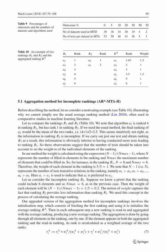
The proportion of test results on datasets/algorithms omitted is a parameter of the method.Here we use the values shown in Table 9. We use the same meta-dataset described earlierin this article. This dataset was used to obtain a new one in which the test results of somedatasets, chosen at random, would be obliterated. The resulting dataset was used to constructthe average ranking. Each ranking was then used to construct a loss-time curve. The wholeprocess was repeated 10 times. This way we would obtain 10 loss-time curves, which wouldbe aggregated into a single loss-time curve. Our aim is to upgrade the average rankingmethod to be able to deal with incomplete rankings. The enhanced method (AR*-MTA-H) isdescribed in the next section. It can be characterized as a heuristic method of aggregation ofincomplete rankings that uses weights of ranks. Later it is compared to the classical approach(AR*-MTA-B), that serves as a baseline here. This method is based on the original Borda’smethod (Lin 2010) and is commonly used by many researchers.
123
Mach Learn (2018) 107:79–108 99
Table 9 Percentages ofomissions and the numbers ofdatasets and algorithms used
Omissions % 0 5 10 20 50 90 95
No of datasets used in MTD 38 36 34 30 19 4 2
No of tests per dataset in MTA 53 50 48 43 26 5 3
Table 10 An example of tworankings R1 and R2 and theaggregated ranking RA
R1 Rank R2 Rank RA Rank Weight
a1 1 a2 1 a1 1.67 1.2
a3 2 a1 2 a3 2 1
a4 3 a4 3 1
a2 4 a2 3.5 1.2
a6 5 a6 5 1
a5 6 a5 6 1
5.1 Aggregation method for incomplete rankings (AR*-MTA-H)
Before describing themethod, let us consider amotivating example (see Table 10), illustratingwhy we cannot simply use the usual average ranking method (Lin 2010), often used incomparative studies in machine learning literature.
Let us compare the rankings R1 and R2 (Table 10). We note that algorithm a2 is ranked 4in ranking R1, but has rank 1 in ranking R2. If we used the usual method, the final ranking ofa2 would be the mean of the two ranks, i.e. (4+1)/2=2.5. This seems intuitively not right, asthe information in ranking R2 is incomplete. If we carry out just one test and obtain rankingR2 as a result, this information is obviously inferior to having conducted more tests leadingto ranking R1. So these observations suggest that the number of tests should be taken intoaccount to set the weight to of the individual elements of the ranking.
In ourmethod theweight is calculated using the expression (N−1)/(Nmax−1), where Nrepresents the number of filled-in elements in the ranking and Nmax the maximum numberof elements that could be filled-in. So, for instance, in the ranking R1, N = 6 and Nmax = 6.Therefore, the weight of each element in the ranking is 5/5 = 1. We note that N − 1 (i.e. 5),represents the number of non-transitive relations in the ranking, namely a1 > a3, a3 > a4, .. ,a6 > a5. Here ai > a j is used to indicate that ai is preferred to a j .
Let us consider the incomplete ranking R2. Suppose we know a priori that the rankingcould include 6 elements and so Nmax = 6, as in the previous case. Then the weight ofeach element will be (N − 1)/(Nmax − 1) = 1/5 = 0.2. The notion of weight captures thefact that ranking R2 provides less information than ranking R1. We need this concept in theprocess of calculating the average ranking.
Our upgraded version of the aggregation method for incomplete rankings involves theinitialization step, which consists of fetching the first ranking and using it to initialize theaverage ranking RA. Then in each subsequent step a new ranking is read-in and aggregatedwith the average ranking, producing a new average ranking. The aggregation is done by goingthrough all elements in the ranking, one by one. If the element appears in both the aggregatedranking and the read-in ranking, its rank is recalculated as a weighted average of the tworanks:
r Ai := r Ai ∗ wAi /(wA
i + wji ) + r j
i ∗ wji /(w
Ai + w
ji ) (7)
123
100 Mach Learn (2018) 107:79–108
Fig. 10 Spearman’s rankcorrelation coefficient betweenrankings for pairs of datasets
Histogram of correlation
correlation
Freq
uenc
y
−0.5 0.0 0.5 1.0
050
100
150
200
where r Ai represents the rank of element i in the aggregated ranking and r ji the rank of the
element i in the ranking j and wAi and w
ji represent the corresponding weights. The weight
is updated as follows:wAi := wA
i + wji (8)
If the element appears in the aggregated ranking, but not in the new read-in ranking, both therank and the weight are kept unchanged.
Suppose the aim is to aggregate the rankings R1 and R2 shown before. The new rank ofa2 will be r A2 = 4 * 1/1.2 + 1*0.2/1.2 = 3.5. The weight will be wA
2 = 1 + 0.2 = 1.2. The finalaggregated ranking of rankings R1 and R2 is RA as shown in Table 10.
5.2 Results on the effects of omissions in the meta-dataset
5.2.1 Characterization of the meta-dataset
We were interested in analyzing different rankings of classification algorithms on differentdatasets used in this work and, in particular, how these differ for different pairs of datasets. Iftwo datasets are very similar, the algorithm rankings will also be similar and, consequently,the correlation coefficient will be near 1. On the other hand, if the two datasets are quitedifferent, the correlation will be low. In the extreme case, the correlation coefficient will be−1 (i.e. one ranking is the inverse of the other). So the distribution of pairwise correlationcoefficients provides an estimate of how difficult the meta-learning task is.
Figure 10 shows a histogram of correlation values. The histogram is accompanied byexpected value, standard deviation and coefficient of variation calculated as the ratio ofstandard deviation to the expected value (mean) (Witten and Frank 2005). These measuresare shown in Table 11.
5.2.2 Study of accuracy-based rankings and one paradox
Ranking methods use a particular performance measure to construct an ordering of algo-rithms. Some commonly used measures of performance are accuracy, AUC or A3R that
123
Mach Learn (2018) 107:79–108 101
Table 11 Measures characterizing the histogram of correlations in Fig. 10
Measure % Expected value SD Coefficient of variation
Value 0.5134 0.2663 51.86%
Table 12 Mean interval loss(MIL) values for differentpercentage of omissions
Method % Omissions
0 5 10 20 50 90 95
AR*-MTD 22.11 21.09 20.66 20.12 19 17.92 15.15
combines accuracy and runtime discussed in Sect. 3.3. In the first study we have focusedsolely on the average ranking based on accuracy. When studying how omissions of tests ondatasets affect rankings and the corresponding loss time curves, we became aware of oneparadox that can arise under certain conditions. This paradox can be formulated as follows:
Suppose we use tests of a given set of algorithms on a set of M (N) datasets leading toM (N) accuracy-based rankings. Suppose the M (N) rankings are aggregated to construct theaverage ranking. Suppose that M > N (for instance, consider M=10 and N=1). Let ARM
represent the average ranking elaborated on the basis M rankings obtained on the respectiveM datasets. We can then expect that MIL of the variant ARM would be lower (better) thanthe MIL of ARN . However, we have observed that this was exactly the other way round.
Table 12 provides evidence for the observation above. When all datasets are used toconstruct the average ranking (omissions are 0%) the MIL is 22.11. When only 5% areused (omissions are 95%), the MIL value is lower, i.e. 15.15. In other words, using moreinformation leads to worse results!
Our explanation for this paradox is as follows. The accuracy-based average ranking ordersthe algorithms by accuracy. If we use several such rankings constructed on different datasets,we can expect that we get an ordering where the algorithms with high accuracy on manydatasets will appear in the initial positions of the ranking. These algorithms tend to be slowerthan the ones that require less time to train. So if we use this ranking and use loss timecurves in the evaluation, we need to wait a long time before the high-accuracy algorithmsget executed. This does not happen so much if use a ranking constructed on fewer datasets.
We have carried out additional experiments that support this explanation. First, if we usejust test curves, where each test lasts one unit of time, the paradox disappears. Also, if weuse A3R to rank the algorithms, again the problem disappears. In these situations we can seethat if we use more information, the result is normally better.
In conclusion, to avoid the paradox, it is necessary to use a similar criterion both in theconstruction of rankings and in the process of loss curve construction.
5.2.3 Study of AR* ranking methods and the results
In the second study we have focused on AR*. Table 13 presents the results for the alternativesAR*-MTD, AR*-MTA-H and AR*-MTA-B in terms of mean interval loss (MIL). All loss-time curves start from the initial loss of the default classification. This loss is calculatedas the difference in performance between the best algorithm and the default accuracy foreach dataset. The default accuracy is calculated in the usual way, by simply predicting the
123
102 Mach Learn (2018) 107:79–108
Table 13 Mean interval loss (MIL) values for different percentage of omissions
Fig. 11 Comparison of AR*-MTA-H with AR*-MTD and the baseline method AR*-MTA-B for 90% of omis-sions
Fig. 12 Results of Nemenyi test, variants of the meta-learners that are connected by a horizontal line arestatistically equivalent
majority class for the dataset in question. The values for the ordinary average rankingmethod,AR*-MTA-B, are also shown, as this method serves as a baseline.
Figure 11 shows the loss-time curves for the three alternatives when the number of omis-sions is 90%. Not all loss-time curves are shown, as the figure would be rather cluttered.
Our results show that the proposed average ranking method AR*-MTA-H achieves betterresults than the baselinemethodAR*-MTA-B.Wenote also that although the proposedmethodAR*-MTA-H achieves comparable results to AR*-MTD for many values of the percentagedrop (all values up to about 50%). Only when we get to rather extreme values, such as 90%,the difference is noticeable. Still, the differences between our proposed variant AR*-MTA-Hand AR*-MTD are smaller than the differences between AR*-MTA-B and AR*-MTD.
123
Mach Learn (2018) 107:79–108 103
These above observations are supported also by the results of a statistical test. The val-ues shown in Table 13 were used to conduct a Nemenyi test and the result is shown inFig. 12. These results indicate that the proposed average ranking method is relatively robustto omissions.
6 Conclusions
Upgrading AT and AR methods to be more effectiveIn this paper we addressed an approach for algorithm selection where the recommendation
is presented in the form of a ranking. The work described here extends two existing methodsdescribed earlier in the literature. The first one was average ranking (AR) and the secondactive testing (AT).
The first method (AR) is a rather simple one. It calculates an average ranking for allalgorithms over all datasets. We have shown how to upgrade this method to incorporatethe measure A3R that combines accuracy and run time. The novelty here lies in the use ofA3R, instead of just accuracy. The second method (AT) employs tests to identify the mostpromising candidates, as its aim is to intelligently select the next algorithm to test on the newdataset. We have also shown how this method can be to upgraded to incorporate the measureA3R that combines accuracy and runtime.
Establishing the correct balance between accuracy and runtimeWe have also investigated the issue of how to establish the correct balance between accu-
racy and runtime. Giving too much weight to time would promote rather poor algorithmsand hence time could be wasted. Giving too little weight to time would work in the oppositedirection. It would promote tests on algorithms which exhibit good performance in general,but may occasionally fail. Unfortunately, such algorithms tend to be rather slow and so theirincorporation early in the testing process may actually delay the process of identifying goodalgorithms early.
It is thus necessary to establish the correct balance between the weight given to accuracyand theweight given to time.Aswe have shown in Sect. 3.3.2, this can be done by determiningan appropriate setting for parameter P used within function A3R that combines accuracy andruntime. One rather surprising consequence of this is the following: if the user wished toimpose his preference regards the relative importance of accuracy and runtime, he/she wouldprobably end up with a worse result than the one obtained with our setting.
Evaluation methodology using loss-time curvesThe experimental results were presented in the form of loss-time curves. This represen-
tation, where time is represented on a logarithmic scale, has the following advantages. First,it stresses the losses at the beginning of the curve, corresponding to the initial tests. Thisis justified by the fact that users would normally prefer to obtain good recommendations asquickly as possible.
We note that testing without a cut-off on time (budget) is not really practicable, as users arenot prepared to wait beyond a given limit. On the other hand, many applications may allowthat results come only after some small amount of time. This is why here we focused on theselection process within a given time interval. Having a fixed time interval has advantages,as it is possible to compare different variants just by comparing the mean interval loss (MIL).
The results presented earlier, see Sect. 4.3, show that the upgraded versions of AR* andAT* lead to much better results in terms of mean loss values (MIL) than their accuracy-based
123
104 Mach Learn (2018) 107:79–108
counterparts. In other words, the incorporation of both accuracy and runtime into themethodspays off.
Disastrous results of AR0 and a paradox identifiedWe have shown that if we do not incorporate both accuracy and runtime, the variant
AR0 that uses only accuracy leads to disastrous results in terms of MIL. We have providedan explanation for this phenomenon and drawn attention to an apparent paradox, as moreinformation seems to lead to worse results.
Comparison of AT* and AR* methodsWhen comparing theAT* andAR*methods,we note that bothmethods lead to comparable
results. We must keep in mind, however, that our meta-dataset included test results on 53algorithms only. If more candidate algorithms were used, we expect that AT* method wouldlead to better results that AR*.
The effects of incomplete test results on AR* methodWehave also investigated the problemof how the process of generating the average ranking
is affected by incomplete test results by describing a relatively simple method, AR*-MTA-H,that permits to aggregate incomplete rankings. We have also proposed a methodology that isuseful in the process of evaluating our aggregation method. This involves using a standardaggregation method AR*-MTD on a set of complete rankings, but whose number is decreasedfollowing the proportion of omissions in the incomplete rankings. As we have shown, theproposed aggregation method achieves quite comparable results and is relatively robust toomissions in test results in the test data. We have shown that a percentage drop of up to 50%does notmakemuch difference. As the incompletemeta-dataset does not affectmuch the finalranking and the corresponding loss, this could be explored in future design of experiments,when gathering new test results.
6.1 Discussion and future work
In this section we present some suggestions on what could be done in future work.
Verifying the conjecture regarding AT*In Sect. 4.3 we have compared the two best variants - AT* and AR*. We have shown
that the results obtained with the AT* variant are slightly worse than those obtained usingAR*. However, the two results are statistically equivalent and it is conceivable that if thenumber of algorithms or their variants were increased, the AT* method could win over AR*.Experiments should be carried out to verify whether this conjecture holds. Also, we plan tore-examine the AT method to see if it could be further improved.
Would the best setting of P transfer to other datasets?An interesting question is how stable the best setting for the parameter P (parameter used
within A3R) is. This could be investigated in the following manner. First we can gather alarge set of datasets and draw samples of datasets of fixed size at random.Wewould establishthe optimum Pi for sample i and then determine what we would be the loss on sample j ifPi were used, rather than the optimized value Pj .
How does P vary for different budgets?Another question is whether the optimum value of P varies much if the budget (Tmax ) is
altered. A more general question involves the interval Tmin - Tmax . Further studies should becarried out, so that these questions could be answered.
123
Mach Learn (2018) 107:79–108 105
Applying AT both to algorithm selection and hyper-parameter tuningWe should investigate whether the ATmethod can be extended to handle both the selection
of learning algorithms and parameter settings. This line ofworkmay require the incorporationof techniques used in the area of parameter settings (e.g. [?], among others).
Combining AT with classical approaches to meta-learningAnother interesting issue is whether the AT approach could be extended to incorporate the
classical dataset characteristics and whether this would be beneficial. Earlier work (Leite andBrazdil 2008) found that the AT approach achieves better results than classical meta-modelsbased on dataset characteristics. More recently, it was shown (Sun and Pfahringer 2013)that pairwise meta-rules were more effective than the other ranking approaches. Hence, itis likely that the AT algorithm could be extended by incorporation information of datasetcharacteristics and pairwise meta-rules.
Leave-one-out CV versus k-fold cross-validationAll methods discussed in this paper were evaluated using the leave-one-out cross-
validation (LOO-CV). All datasets except one were used to refine our model (e.g. AR).The model was then applied to the dataset that was left out and evaluated by observing theloss curve. We have opted for this method, as our meta-dataset included test results on amodest number of datasets (39). As LOO-CV may suffer from high variance, 10-fold CVcould be used in future studies.
Study of the effects of incomplete meta-datasetsIn most work on meta-learning it is assumed that the evaluations to construct the meta-
dataset can be carried out off-line and hence the cost (time) of gathering this data is ignored.In future work we could investigate approaches that permit to consider also the costs (time)of off-line tests. Their cost (time) could be set to some fraction of the cost of on-line test (i.e.tests on a new dataset), but not really ignored altogether. The approaches discussed in thispaper could be upgraded so that they would minimize the overall costs.
Acknowledgements The authors wish to express our gratitude to the following institutions which have pro-vided funding to support this work: Federal Government of Nigeria Tertiary Education Trust Fund underthe TETFund 2012 AST$D Intervention for Kano University of Science and Technology, Wudil, KanoState, Nigeria for PhD Overseas Training; FCT/MEC through PIDDAC and ERDF/ON2 within projectNORTE-07-0124-FEDER-000059 and through the COMPETE Programme (operational programme for com-petitiveness) and by National Funds through the FCT Portuguese Foundation for Science and Technologywithin project FCOMP-01-0124-FEDER-037281; Grant 612:001:206 from the Netherlands Organisation forScientific Research (NWO). We wish to express our gratitude to all anonymous referees for their detailedcomments which led to various improvements of this paper. Also, our thanks to Miguel Cachada for readingthrough the paper and his comments and in particular one very useful observation regarding the AT method.
123
106 Mach Learn (2018) 107:79–108
A Algorithm ranks
See Table 14.
Table 14 Algorithms used in the experiment and their ranks ordered usingAR*.All classifiers as implementedin Weka 3.7.12. For full details, see https://www.openml.org/s/37
Abdulrahman, S. M., & Brazdil, P. (2014). Measures for combining accuracy and time for meta-learning.Meta-Learning and Algorithm Selection Workshop at ECAI, 2014, 49–50.
Brazdil, P. & Soares, C. (2000). A Comparison of ranking methods for classification algorithm selection. InMachine Learning: ECML 2000, pp. 63–75. Springer.
Brazdil, P., Soares, C., & da Costa, J. P. (2003). Ranking learning algorithms: Using IBL and meta-learningon accuracy and time results. Machine Learning, 50(3), 251–277.
Brazdil, P., Carrier, C . G., Soares, C., & Vilalta, R. (2008).Metalearning: Applications to data mining. Berlin:Springer.
Demšar, J. (2006). Statistical comparisons of classifiers over multiple data sets. The Journal of MachineLearning Research, 7, 1–30.
Fedorov, V . V. (1972). Theory of optimal experiments. Cambridge: Academic Press.Feurer, M., Springenberg, T. & Hutter, F. (2015). Initializing bayesian hyperparameter optimization via meta-
learning. In Proceedings of the Twenty-Ninth AAAI Conference on Artificial Intelligence, January 2015.Fürnkranz, J.&Petrak, J. (2001).An evaluation of landmarking variants. InWorkingNotes of the ECML/PKDD
2000Workshop on Integrating Aspects of DataMining, Decision Support andMeta-Learning, pp. 57–68.Hall, M., Frank, E., Holmes, G., Pfahringer, B., Reutemann, P., &Witten, I. H. (2009). TheWEKAdatamining
software: An update. ACM SIGKDD Explorations Newsletter, 11(1), 10–18.Jankowski, N. (2013). Complexity measures for meta-learning and their optimality. In Algorithmic Probability
and Friends. Bayesian Prediction and Artificial Intelligence., pp. 198–210.Leite, R. & Brazdil, P. (2008). Selecting classifiers using meta-learning with sampling landmarks and data
characterization. InProceedings of the 2ndPlanning to LearnWorkshop (PlanLearn) at ICML/COLT/UAI2008, pp. 35–41.
Leite, R. & Brazdil, P. (2010). Active testing strategy to predict the best classification algorithm via samplingand metalearning. In ECAI, pp. 309–314.
Leite,R., Brazdil, P.&Vanschoren, J. (2012). Selecting classification algorithmswith active testing. InMachineLearning and Data Mining in Pattern Recognition, pp. 117–131. Springer.
123
108 Mach Learn (2018) 107:79–108
Li, L., Chu, W., Langford, J. & Schapire, R. E. (2010). A contextual-bandit approach to personalized newsarticle recommendation. In Proceedings of 19th WWW, pp. 661–670. ACM.
Lin, S. (2010). Rank aggregation methods. WIREs Computational Statistics, 2, 555–570.Long, B., Chapelle, O., Zhang, Y., Chang, Y., Zheng, Z. & Tseng, B. (2010). Active learning for ranking
through expected loss optimization. In Proceedings of the 33rd International ACM SIGIR Conferenceon Research and Development in Information Retrieval, pp. 267–274. ACM.
Neave, H. R., & Worthington, P. L. (1988). Distribution-free Tests. London: Unwin Hyman.Pfahringer, B., Bensusan, H. & Giraud-Carrier, C. (2000). Tell me who can learn you and I can tell you who
you are: Landmarking various learning algorithms. In Proceedings of the 17th International Conferenceon Machine Learning, pp. 743–750.
Pihur, V., Datta, S., & Datta, S. (2009). RankAggreg, an R package for weighted rank aggregation. BMCBioinformatics, 10(1), 62.
Prudêncio, R. B. & Ludermir, T. B. (2007). Active selection of training examples for meta-learning. In 7thInternational Conference on Hybrid Intelligent Systems, 2007. HIS 2007., pp. 126–131. IEEE.
Rice, J. R. (1976). The algorithm selection problem. Advances in Computers, 15, 65–118.Smith-Miles, K . A. (2008). Cross-disciplinary perspectives on meta-learning for algorithm selection. ACM
Computing Surveys (CSUR), 41(1), 6:1–6:25.Sun, Quan, & Pfahringer, B. (2013). Pairwise meta-rules for better meta-learning-based algorithm ranking.
Machine Learning, 93(1), 141–161.van Rijn, J. N., Abdulrahman, S. M., Brazdil, P. & Vanschoren, J. (2015). Fast algorithm selection using
learning curves. In Advances in Intelligent Data Analysis XIV, pp. 298–309. Springer.Vanschoren, J., van Rijn, J. N., Bischl, B., & Torgo, L. (2014). OpenML: Networked science in machine
learning. ACM SIGKDD Explorations Newsletter, 15(2), 49–60.Witten, I . H., & Frank, E. (2005).Data mining: Practical machine learning tools and techniques. Burlington:
Morgan Kaufmann.Xu, L., Hutter, F., Hoos, H., & Leyton-Brown, K. (2011).Hydra-MIP: Automated algorithm configuration and
selection for mixed integer programming. In RCRAworkshop on Experimental Evaluation of Algorithmsfor Solving Problems with Combinatorial Explosion at the International Joint Conference on ArtificialIntelligence (IJCAI)