SPENDING ON SOCIAL WELFARE PROGRAMS IN RICH AND POOR STATES Contract # 282-98-0016 Task Order #34 Final Report Appendix A Prepared for: Department of Health and Human Services Assistant Secretary for Planning and Evaluation Prepared by: The Lewin Group and its subcontractor The Nelson A. Rockefeller Institute of Government June 3, 2004
Transcript
SPENDING ON SOCIAL WELFARE PROGRAMS IN RICH AND POOR STATES Contract # 282-98-0016 Task Order #34
Final Report
Appendix A
Prepared for: Department of Health and Human Services Assistant Secretary for Planning and Evaluation
Prepared by: The Lewin Group and its subcontractor
The Nelson A. Rockefeller Institute of Government
June 3, 2004
SPENDING ON SOCIAL WELFARE PROGRAMS IN RICH AND POOR
STATES Contract # 282-98-0016
Task Order #34
Final Report
Appendix A
Prepared for: Department of Health and Human Services
Assistant Secretary for Planning and Evaluation
Prepared by: The Lewin Group and its subcontractor
The Nelson A. Rockefeller Institute of Government
June 30, 2004
Table of Contents
APPENDIX A...............................................................................................................................................................1 THEORETICAL FOUNDATIONS ....................................................................................................................................1 FULL MODEL SPECIFICATIONS AND RESULTS ............................................................................................................4
Appendix A: Theoretical Foundations
APPENDIX A
In this Appendix, we set out the theoretical foundation for the 50-state econometric model and provide more extensive estimates of model parameters.
Theoretical Foundations
Following McGuire (1978) we develop an empirical model of spending by state and local governments. The decision-makers are assumed to maximize a general utility or preference function defined in terms of public and private goods. Public spending on specified activities is determined in part by the relative marginal social utility placed on that category by the state. Both state fiscal capacity and federal grants become part of the state’s budget constraint. Economic conditions within each state are explanatory variables because they determine the relative social utility (or “need”) of spending on specified activities.
A Stone-Geary specification for the preference function1 leads to a series of linear expenditure functions in which per capita total state and local spending on a specified public function is a function of several explanatory variables, including per capita personal income, per capita federal grants, and a number of variables designed to capture the relative need of the states for social welfare spending.
This type of model allows us to focus on how states with different needs for social welfare spending respond to changes in explanatory variables such as fiscal capacity, and the availability of federal grants. It will also allow us to explore how fiscal capacity itself affects state spending on social welfare and other functions.
Our basic (per capita) budget constraint for spending on a particular category of public activity in the combined state-local system was taken to be the sum of per capita personal income (PCPI) and per capita federal grants for that type of spending. If state-local needs were constant (or independent of the other explanatory variables), and federal grants had only income effects2, per capita spending would be a simple linear function of PCPI plus federal grants per capita with a series of dummy variables to represent state effects. That is:
S = α + β R + Σ δjDj + Σ λk Xk
where S = per capita spending on a particular category of spending
R = per capita resources for spending on that category
Dj = a dummy variable having the value 1 if the observation is for the jth state, and 0, otherwise; and
1 See McGuire (1978) and Appendix A for details. 2 In this formulation, the price effects of federal grants induced by matching ratios is not explicitly modeled.
1
Appendix A: Theoretical Foundations
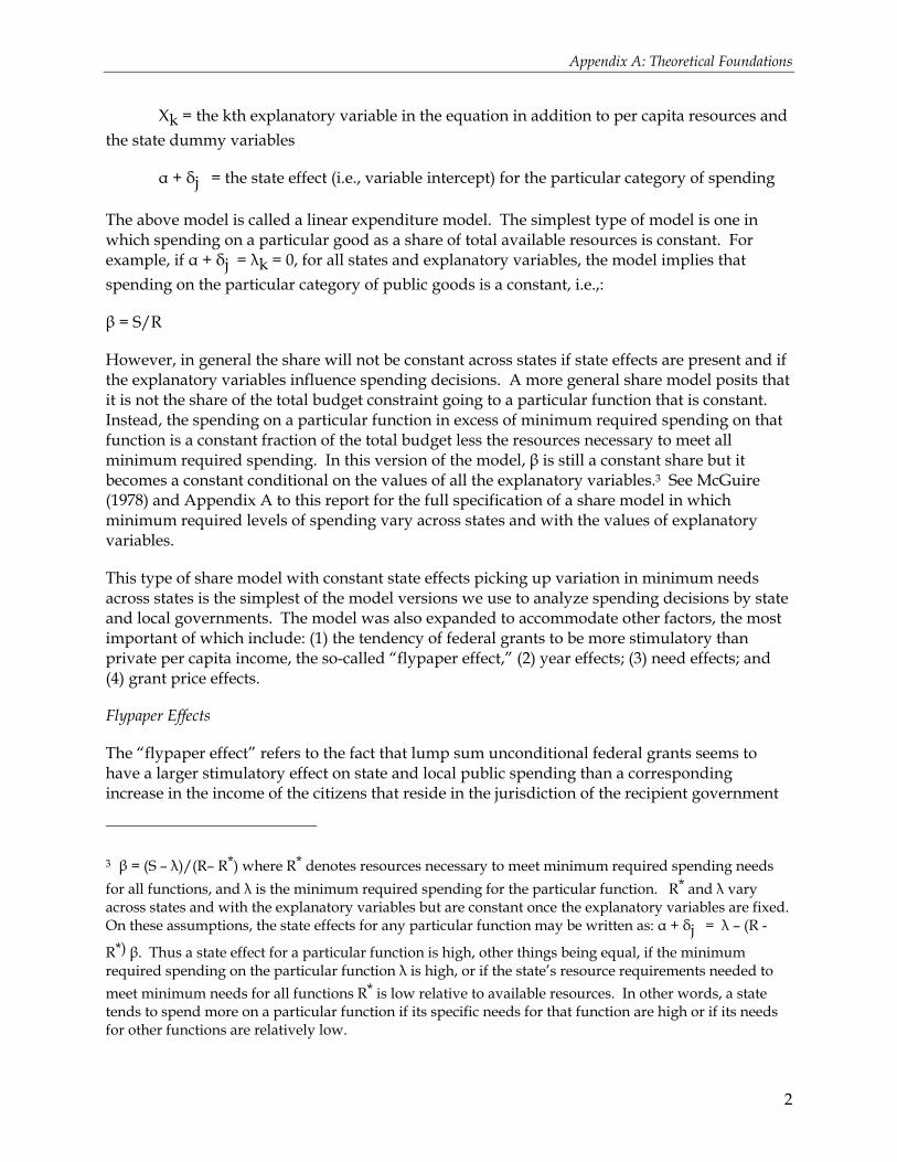
Xk = the kth explanatory variable in the equation in addition to per capita resources and the state dummy variables
α + δj = the state effect (i.e., variable intercept) for the particular category of spending
The above model is called a linear expenditure model. The simplest type of model is one in which spending on a particular good as a share of total available resources is constant. For example, if α + δj = λk = 0, for all states and explanatory variables, the model implies that spending on the particular category of public goods is a constant, i.e.,:
β = S/R
However, in general the share will not be constant across states if state effects are present and if the explanatory variables influence spending decisions. A more general share model posits that it is not the share of the total budget constraint going to a particular function that is constant. Instead, the spending on a particular function in excess of minimum required spending on that function is a constant fraction of the total budget less the resources necessary to meet all minimum required spending. In this version of the model, β is still a constant share but it becomes a constant conditional on the values of all the explanatory variables.3 See McGuire (1978) and Appendix A to this report for the full specification of a share model in which minimum required levels of spending vary across states and with the values of explanatory variables.
This type of share model with constant state effects picking up variation in minimum needs across states is the simplest of the model versions we use to analyze spending decisions by state and local governments. The model was also expanded to accommodate other factors, the most important of which include: (1) the tendency of federal grants to be more stimulatory than private per capita income, the so-called “flypaper effect,” (2) year effects; (3) need effects; and (4) grant price effects.
Flypaper Effects
The “flypaper effect” refers to the fact that lump sum unconditional federal grants seems to have a larger stimulatory effect on state and local public spending than a corresponding increase in the income of the citizens that reside in the jurisdiction of the recipient government
3 β = (S – λ)/(R– R*) where R* denotes resources necessary to meet minimum required spending needs for all functions, and λ is the minimum required spending for the particular function. R* and λ vary across states and with the explanatory variables but are constant once the explanatory variables are fixed. On these assumptions, the state effects for any particular function may be written as: α + δj = λ – (R -
R*) β. Thus a state effect for a particular function is high, other things being equal, if the minimum required spending on the particular function λ is high, or if the state’s resource requirements needed to meet minimum needs for all functions R* is low relative to available resources. In other words, a state tends to spend more on a particular function if its specific needs for that function are high or if its needs for other functions are relatively low.
2
Appendix A: Theoretical Foundations
(Gramlich 1977; Hines and Thaler, 1995; Gamkhar and Oates, 1996) This contradicts established theory that indicates that lump sum grants to a locality should have allocative and distributive effects no different than if the grant were distributed directly to the residents of the locality (Bradford and Oates, 1971). Empirical research has strongly established the existence of such an effect, at least in response to increases in federal grants.
Theoretical explanations for the “flypaper effect” vary widely. For example, Hines and Thaler (1995) posit explanations ranging from individuals not recognizing the fungibility of money to the median voter bearing a smaller than average fraction of the tax burden.
Our approach to accommodating the flypaper effect was to partition the budget constant independent resource variable R into two variables, one that reflects private per capita income and one that reflects per capita federal grants.
Year Effects
Year effects refer to the fact that the minimum needs that drive state-local spending decisions may vary from year to year. We dealt with this by specifying models in which we added dummy variables for each year, to effectively shift up and down the intercept term over time to accommodate time variant effects.
Particular Needs
We also attempted to model the need effects. Instead of allowing minimum needs simply to vary across states through the state effects, we also introduced variables such as poverty, unemployment, population density and percent urban to explore whether or not states behaved as though they had stable needs functions.
Price Effects
A matching grant under which the federal government agrees to match state spending at some rate effectively lowers the “price” to the state or local decision-maker (in terms of local resources) of directing resources to the aided governmental function For example, if the federal government agrees to pay $0.60 for every dollar of state spending on an activity, then the state’s cost (in its own resources) to finance $1 in spending on that activity has fallen to $(1-0.60) or $0.40. 4
4 Much of the research reported is on the issue of how strongly this price effect stimulates state spending on aided activities. The literature contrasts non-matching grants, which are thought to have only income effects, with matching grants, which are thought to have both price and income effects. It also discusses revenue sharing which carries no restrictions on how grant monies are to be used with restricted grants that must be used for designated purposes. Revenue-sharing is thought to have a pure income effect, but no price effect. Restricted unmatched grants are thought to have only income effects if the state would spend at least as much as the grant amount in the absence of the grant (so that the restriction is not binding). However, if the grant restriction is binding, the restricted grant has an implied price effect as well as an income effect. In general, an unrestricted revenue-sharing grant to the states would be expected to reduce state spending as the states would use the money to substitute for spending from their
3
Appendix A: Theoretical Foundations
Following McGuire (1978), we attempted to incorporate the “price” effects of grants into the analysis. This was done formally by assuming that some fraction of a grant was effectively unrestricted, i.e., the grant had a pure income effect through the budget constraint, and the remainder of the grant had only a price effect and thus did not enter the budget constraint. This leads to a more complex model structure in which the ratio of federal grants for a particular category of public functions to total state-local spending enter the linear expenditure function interacted with other variables. The full model is specified below. Another simpler approach to take account of price effects is to add year dummy variables to the regression, which was done in Model 1 without formal consideration of price effects. The results for Model 1D are presented also in the text of this report. The combination of year and state effects will capture much of the variation in changes in grant conditions in particular states at particular times.
Full Model Specifications and Results
Our model is based on the theoretical work by McGuire (1978), in which he modeled state-local spending on education and non-education functions. However, we have certain data problems not present in McGuire’s estimation. He estimated his model on Census data that permitted him to have the same level of aggregation in his data on intergovernmental revenues as in his data on state-local spending, and he used a simple two category model of public activities. On the other hand, our challenge was to press the econometric modeling to accommodate five categories of public goods: cash assistance, Medicaid, other social welfare, public hospitals and non-public hospital non-social welfare spending, while the data on intergovernmental revenues used to estimate federal grant levels was available only for “social welfare spending” and “non-social welfare” spending.
To accommodate this restriction in the data, we needed to redefine our dependent variable as total state-local spending rather than state-local spending from all sources. Furthermore, McGuire deals with the so-called “flypaper effect,” but by a very ad hoc method, namely, he includes an extra parameter in his equations which is not in the preference function. But this is inconsistent with optimization of the preference function and essentially forces an empirical result that allows the effect of private resources and grant resources on state-local spending to be different. We take a slightly different approach and allow the flypaper effect to shift linearly the minimum subsistence level of spending by whether the source of the income is federal grants or private income.
We set forth the model for two public goods first and then generalize it to four public goods, which is the models we use primarily in the report. However, because the mathematics is rather tedious, it is easier to follow if we use the two good model and then explain how it can be extended to four public goods. For two public goods (Qs, social welfare spending, and Qo, non-social welfare spending, and a private good Y), the Stone-Geary function to be maximized is:
own sources. However, either matching formulas or restrictions can reduce or eliminate this displacement effect. Federal matching serves as a “carrot,” rewarding states that spend more in designated areas, while restrictions act as a “stick,” taking away funds if the conditions (e.g. maintenance of effort) are not met.
4
Appendix A: Theoretical Foundations
U = (Y – λy)βy (Qs – λs)βs (Qo – λo)βo, (1)
where λy, λs, and λo, are the minimum required spending for private goods, social welfare public goods, and non-social welfare public goods, respectively, and βy, βs, and βo are the relative utility parameters of the utility function. Without loss of generality, the βs can be assumed to equal 1.5
Relative prices in the economy are assumed to be fixed, but the price of each of the public goods is assumed to be affected by the terms of the federal grant aiding the particular good. If all of a federal grant were to lower the price of spending the effective price would fall from 1 (i.e., one dollar of state-local spending costs one dollar) to 1-M, where M is federal share of total spending, i.e., M =G/Q, where Q is total spending on the aided function (G+L), and G and L are federal and state-local spending, respectively. In our model, the price of the aided good will be allowed to vary from 1 to 1-M depending on the degree to which grants have price effects or have pure income effects. Specifically, the price of the aided function is stated as
p = 1 + (θ - 1) M = (L + θG)/(L+G) (2)
with θ expected to vary between 1 and 0. When θ = 1 the grant has no effect on price, and p = 1. When θ =0, p = 1-M. The lower the price, the more the states and localities are expected to spend from their own resources on the aided function.
The social preference function is maximized subject to a budget constraint:
RT = Y + psQs + poQo = RL + θsGs + θoGo, (3)
where the price of private goods is assumed to be 1 (i.e., a numeraire), ps and po are the prices (as defined in (2)) of social welfare public goods and other public goods, respectively, RT is the total public and private resources, Y is spending on private goods, Qs and Qo are total spending (federal, state and local) on social welfare and other public goods, respectively, Gs and Go are federal grants to aid social welfare, and other public functions, respectively, θs and θo are the fractions of federal grants that do not affect prices, for social welfare and non-social welfare functions, respectively, and RL is state-local own resources.
Maximizing the preference function (2) subject to the budget constraint (3) leads to the
5 The β parameters in the utility function can be identified from the linear expenditure functions only to a factor of proportionality. Thus, we do not lose any information by assuming that the parameters sum to unity.
5
Appendix A: Theoretical Foundations
The private spending variable (Y) is determined from the budget constraint RT – psQs – poQo – Y. Solving for Y gives an equation for private spending similar to the two public spending equations:
Y = RL – Ls – Lo = (1 – βy)λy + βyRT - βyλsps - βyλopo (6)
Substituting for RT from equation (3), for ps and po from equation (1), and rearranging terms gives:
f1 = – λoβs(θo – 1) ; f2 = λo (1 – βo)(θo – 1) ; f3 = - λoβy(θo – 1) and f1 + f2 + f3 = 0
We use the above equation as a general model into which we introduce a number of additional restrictions and parameters to test hypotheses.
First, the above model has no flypaper effect because an increase in income affects public spending in the same way whether it arises from local resources or federal grants. The “flypaper effect” refers to the empirical fact that lump sum unconditional federal grants seem to have a larger stimulatory effect on state and local public spending than a corresponding increase in the income of the citizens that reside in the jurisdiction of the recipient government (Gramlich 1977; Hines and Thaler, 1995; Gamkhar and Oates, 1996) This contradicts established theory that indicates that lump sum grants to a locality should have allocative and distributive effects no different than if the grant were distributed directly to the residents of the locality (Bradford and Oates, 1971). Empirical research has strongly established the existence of such an effect, at least in response to increases in federal grants. However, some researchers have found an asymmetric response with the flypaper effect occurring only in response to increases and not in response to decreases in grant levels.
Theoretical explanations for the “flypaper effect” vary widely. For example, Hines and Thaler (1995) posit explanations ranging from individuals not recognizing the fungibility of money to the median voter bearing a smaller than average fraction of the tax burden.
In McGuire’s analysis of educational expenditures, he acknowledges the “flypaper effect” by introducing a parameter П assumed to be greater than one that augments the stimulatory effects of federal grants. This parameter enters the linear spending equations multiplicatively and may be interpreted as increasing the “power” of income received through governmental grants. One problem with this approach in the context of McGuire’s theoretical model is that it compromises the integrity of his optimization scheme. For example, he begins by positing that state and local decision-makers maximize a Stone-Geary social preference function defined in terms of total spending on various goods (education public good, non-education public goods and private goods). However, when he arbitrarily introduces the new parameter into the demand functions, he can no longer solve the optimization problem for private goods. While his optimization conditions still determine spending on the public goods, the magnitude of the flypaper effect determines the spending on private goods. Ideally, one would incorporate the flypaper effect as a feature of a theoretical optimization model.
We take an approach which allows for optimization with respect to all public and private categories of spending. Instead of arbitrarily increasing the stimulation effect of grants of public spending by a factor П, we allow federal grants to affect the minimum required levels of spending for each public good in the model. The grant recipient maximizes a Stone-Geary utility function in which the minimum required spending amounts for each category of public goods is determined by the mix of federal grants and a number of need variables.
Unlike McGuire (1978), we choose to conceptualize the flypaper effect as occurring through the effect of grant income on the minimum required levels of public spending. Because there may be price effects of grants, we need to relate the additional stimulus of a federal grant due to the flypaper effect to the real purchasing power of the grant income if used to fund a specified
7
Appendix A: Theoretical Foundations
category of public spending. Thus, we write the expressions for minimum required public spending levels for social welfare and non-social welfare (λs and λo, respectively) and the minimum required private spending level (λy) as:
There are four П parameters that relate the minimum required levels of spending on social welfare and non-social welfare to the purchasing power of the income effects of the federal grants. The parameter Пij refers to the effect of a grant for the ith spending category on spending on the jth category of public goods. Because we have two categories of public goods, there are four parameters capturing “own” and “cross” effects of grants on public spending. The term in the denominators (1 + (θi - 1) Mi) is the price of spending on the ith public good. The term in the numerators θi Gi is the magnitude of the pure income effect of a federal grant aiding the ith public good. If the flypaper effect does not exist, all four П parameters are zero, and our model is identical to that expressed in equations (10), (11) and (12 ), with the parameters λs0 and λo0 taking the place of parameters λs and λo, respectively. The X variables are variables thought to affect governmental decision-makers’ perceived need for public versus private spending (e.g., unemployment, poverty, etc.).
Substituting (13), (14) and (15) into (10), (11) and (12) gives a linear model with the flypaper parameters and need variables incorporated.
Ls + Gs = a1 + b1RL + c1Go + d1Gs + e1Ms + f1Mo + Σ g1iXi + Σ h1iXi Ms + Σ φ1iXi Mo (16)
Lo + Go = a2 + b2RL + c2Go + d2Gs + e2Ms + f2Mo + Σ g2iXi + Σ h2iXi Ms + Σ φ2iXi Mo (17)
Y = a3 + b3RL + c3Go + d3Gs + e3Ms + f3Mo + Σ g2iXi + Σ h2iXi Ms + Σ φ2iXi Mo (18)
Within this framework, we can estimate a series of models that incorporate various constraints. We report the model results for the four public good model, which is a generalization of the two good model summarized above.6 For this model we will report results for the following special and general cases:
6 The model structure in equations (16) and (17) can be generalized for four public goods to become four equations of the general form::
Li + Gi = ai + bi RL + Σ δj Gj + Σ λj Mj + Σ Σ ξjk Xk Mj where j = 1, …, 4; and k = 1, … n and n is the number of “need” variables in the equation. Equation (18) becomes:
Y = = a5+ b5 RL + Σ δj Gj + Σ λj Mj + Σ Σ ξjk Xk Mj with similar constraints applying to the system. We need only estimate the first four equations because the coefficients in the income equation are linear combinations of the coefficients in the first four equations. In order to estimate the four public good model from the Census data, it was necessary to deal with a major problem posed by data limitations. McGuire’s approach assumes that we have the same level of detail for spending as for intergovernmental grants. Unfortunately, we do not for social welfare spending. The intergovernmental revenue variable used to measure federal grants is available only for the broad aggregates of social welfare spending and non-social welfare spending, while social welfare spending is available for three subcategories of spending; cash assistance, Medicaid, and other social welfare. Therefore, to estimate Models 2 and 3, we needed to assume that the ratio of federal grants for a
9
Appendix A: Theoretical Foundations
• Model 1A: A model with no price effects (all θ = 1), no flypaper effects (all П = 0), and without “need” variables (all λji= 0);
• Model 1B: A model with no price effects (all θ = 1), no flypaper effects (all Пos= 0), but including need variables;
• Model 1C: A model with no price effects (all θ = 1), no need variables, but including flypaper effects; and
• Model 1D: A model with no price effects , including need variables and including flypaper effects.
• Model 2A: A model with no income effects of grants (all θ = 0) (as a consequence, flypaper effects do not exist), and without need variables (all λji=0);
• Model 2B: A model with no income effects of grants (all θ = 0) (as a consequence, flypaper effects do not exist), and including need variables.
• Model 3A: A model with estimated price effects, no flypaper effects (all П = 0), and without “need” variables;
• Model 3B: A model with estimated price effects, including need variables and including flypaper effects.
We estimated each of these models using annual data over the time period 1978 to 2001 for all states, and also separately for four quartiles of states based on average state per capita personal income over the observation period.
Model 1A Specification
Model 1A is the simplest, but least realistic model. It assumes that the grantee government responds to all grants as though they were unconditional, and that grant income affects public spending levels and allocations in the same way as income in the private sector. It also assumes that a state’s “needs” are adequately represented by linear state effects (i.e., allowing the constant term in the regression to be different for each state). The latter assumption would be consistent with unbiased estimates of regression coefficients only if needs were uncorrelated with included independent variables (fiscal capacity and grant levels).
The model reduces to:
Ls + Gs = a1 + b1RL + c1Go + d1Gs (with b1 = c1 = d1 = βs) or Ls + Gs = a1 + b1(RL+ Go + Gs)
subcategory of social welfare to total grants for social welfare was constant. This enabled us to replace Mj
by[Gsw / (Sj + Gj)] which on that assumption is linearly related to Mj = Gj /( Sj + Gj). Since Sj + Gj is observed, although Gj is not, we can estimate the four good model.
10
Appendix A: Theoretical Foundations
Lo + Go = a2 + b2RL + c2Go + d2Gs (with b2 = c2 = d2 = βo) or Ls + Gs = a2 + b2(RL+ Go + Gs)
Y = a3 + b3RL + c3Go + d3Gs (with b3 = c3 = d3 = βy) or Y = a3 + b3(RL+ Go + Gs)
The regression results are shown in Exhibit A-1.
Exhibit A-1 SWS Model 1A Coefficient Estimates With Year Dummies
Variable Adjusted R-
Squared Constant
Per capita total
income CA 0.85 169.11 (10.08) -0.01 (9.31) M 0.83 77.29042 (3.11) 0.003 (3.60)
CA means Cash Assistance, M means Medicaid, OW means Non-health Social Services, PH means Public Hospital Spending, and NSWS means Non-Social Welfare Spending.
Model 1B Specification
11
Appendix A: Theoretical Foundations
Model 1B improves on Model 1A by introducing objective measures of need thought to affect the minimum required spending levels in each state. However, like Model 1A, this model also assumes that governmental decision-makers respond to grant income in the same way as private income, and that all grant income is unconditional.
Ls + Gs = a1 + b1(RL+ Go + Gs) + Σ g1iXi
Lo + Go = a2 + b2(RL+ Go + Gs) + Σ g2iXi
Y = a3 + b3(RL+ Go + Gs) + Σ g3iXi
The regression results for Model 1B are reported in Exhibit A-2.
12
App
endi
x A
: The
oret
ical
Fou
ndat
ions
Exhi
bit A
-2
SWS
Mod
el 1
B C
oeff
icie
nt E
stim
ates
With
Yea
r Dum
mie
s
Varia
ble
Adj
uste
d R
-Squ
ared
C
onst
ant
Fe
dera
l gr
ants
Popu
latio
n D
ensi
ty
U
nem
ploy
men
t pe
r cap
ita
Pove
rty
per
capi
ta
(mov
. av
g)
C
A
0.86
120.
13(6
.63)
0.00
(7.0
3)
0.03
(3.5
6)89
3.64
(7.4
3)-1
3.79
(0.4
6)M
0.
86
85
.51
(3.3
9)0.
00(3
.00)
-0
.17
(14.
12)
823.
77(4
.92)
-51.
51(1
.24)
OW
0.
86
-9
.13
(0.4
1)0.
01(8
.95)
-0
.06
(5.9
8)13
.89
(0.0
9)-3
1.89
(0.8
7)PH
0.
88
23
5.51
(13.
14)
0.00
(0.6
1)
-0.0
7(8
.40)
307.
77(2
.58)
-52.
79(1
.80)
Ove
rall
NSW
S 0.
96
20
82.9
4(8
.12)
0.
12
(14.
95)
0.54
(4
.52)
77
53.8
3 (4
.55)
23
5.55
(0
.56)
CA
0.
88
34
8.46
(9.9
7)
-0.0
1 (7
.46)
0.
02
(2.1
6)
1268
.17
(4.3
4)
1.03
(0
.02)
M
0.89
278.
07(5
.50)
0.
00
(2.3
6)
-0.1
6 (1
0.84
) 18
06.9
3 (4
.27)
-7
9.20
(1
.17)
OW
0.
86
11
0.66
(2.3
8)
0.01
(5
.58)
-0
.06
(4.6
2)
436.
27
(1.1
2)
-47.
49
-(0.
76)
PH
0.86
84.3
2(2
.58)
0.
00
(4.0
3)
-0.0
7 (7
.03)
33
.30
(0.1
2)
-5.3
0 (0
.12)
1
NSW
S 0.
95
42
2.63
(0.5
8)
0.13
(7
.03)
0.
60
(2.8
2)
1301
1.00
(2
.15)
10
69.6
1 (1
.11)
CA
0.
74
-2
64.3
7(3
.65)
0.
01
(2.9
4)
0.41
(3
.60)
12
90.7
2 (4
.37)
53
6.67
(3
.82)
M
0.85
123.
48(1
.76)
0.
00
(0.0
2)
0.03
(0
.23)
11
5.43
(0
.40)
26
5.27
(1
.95)
OW
0.
87
-9
7.11
(1.3
6)
0.01
(4
.36)
-0
.30
(2.6
6)
92.9
5 (0
.32)
67
.09
(0.4
9)
PH
0.90
394.
37(7
.55)
-0
.01
(3.4
4)
-0.2
8 (3
.41)
60
8.31
(2
.85)
63
.69
(0.6
3)
Qua
rtile
2
NSW
S 0.
94
36
35.6
1(5
.86)
0.
06
(3.2
2)
2.48
(2
.56)
11
168.
00
(4.4
1)
689.
43
(0.5
7)
13
App
endi
x A
: The
oret
ical
Fou
ndat
ions
Exhi
bit A
-2 (c
ontin
ued)
SW
S M
odel
1B
Coe
ffic
ient
Est
imat
es W
ith Y
ear D
umm
ies
Varia
ble
Adj
uste
d R
-Squ
ared
C
onst
ant
Fe
dera
l gr
ants
Popu
latio
n D
ensi
ty
U
nem
ploy
men
t pe
r cap
ita
Pove
rty
per
capi
ta
(mov
. av
g)
C
A
0.82
-67.
97(2
.14)
0.
00
(2.3
7)
0.92
(6
.47)
46
4.71
(2
.89)
17
8.59
(3
.24)
M
0.84
-32.
05(0
.49)
0.
01
(3.6
2)
-0.0
1 (0
.03)
57
5.61
(1
.74)
11
7.18
(1
.03)
OW
0.
83
22
9.28
(3.4
8)
0.01
(2
.62)
-2
.31
(7.8
3)
494.
09
(1.4
8)
-252
.43
(2.2
1)
PH
0.88
-9.4
4(0
.16)
0.
00
(0.3
0)
0.10
(0
.37)
-3
37.0
2 (1
.15)
-5
9.03
(0
.59)
3
NSW
S 0.
96
24
05.2
7(6
.84)
0.
08
(5.8
8)
-0.4
8 (0
.31)
65
10.2
1 (3
.65)
-2
212.
71
(3.6
2)
CA
0.
36
59
.35
(1.1
7)
0.00
(2
.22)
1.
09
(3.3
0)
176.
84
(0.7
6)
68.3
1 (1
.16)
M
0.81
-46.
44(0
.47)
0.
01
(2.6
1)
0.04
(0
.06)
-4
42.1
9 (0
.99)
42
2.12
(3
.73)
OW
0.
79
76
.57
(1.4
9)
0.00
(1
.82)
-0
.31
(0.9
2)
-339
.21
(1.4
5)
26.3
1 (0
.44)
PH
0.95
-224
.76
(4.8
0)
0.00
(0
.99)
2.
97
(9.8
0)
283.
29
(1.3
3)
93.6
1 (1
.73)
Qua
rtile
4
NSW
S 0.
95
20
63.0
4(4
.23)
0.
02
(0.8
5)
15.2
9 (4
.84)
-4
887.
97
(2.1
9)
157.
56
(0.2
8)
CA
mea
ns C
ash
Ass
ista
nce,
M m
eans
Med
icai
d, O
W m
eans
Non
-hea
lth S
ocia
l Ser
vice
s, P
H m
eans
Pub
lic H
ospi
tal S
pend
ing,
and
NS
WS
mea
ns N
on-S
ocia
l W
elfa
re S
pend
ing.
14
Appendix A: Theoretical Foundations
Model 1C Specification
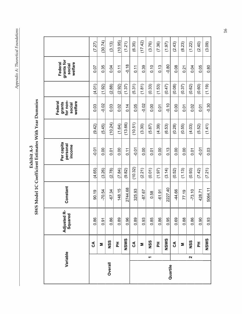
Model 1C is our first attempt to incorporate so-called “flypaper” effects. We still have only income effects without incorporating the price effects of grants, but we allow the effect on federal grants on spending allocation to be different depending on the source of the income. In particular, it is believed that, quite aside from price effects, federal grants have a stronger effect on public spending than on private spending. Model 1C omits need variables. The model can be written as:
Ls + Gs = a1 + b1(RL+ Go + Gs) + (c1 - b1) Go + (d1 - b1) Gs with c1 - b1 > 0, d1 - b1 > 0
Lo + Go = a2 + b2(RL+ Go + Gs) + (c2 – b2) Go + (d2 – b2) Gs with c2 – b2 > 0, d2 – b2 > 0
Y = a3+ b3(RL+ Go + Gs) + (c3 – b3) Go + (d3 – b3) Gs with c3 – b3 < 0, d3 – b3 < 0
The regression results are reported in Exhibit A-3.
15
App
endi
x A
: The
oret
ical
Fou
ndat
ions
Exhi
bit A
-3
SWS
Mod
el 1
C C
oeff
icie
nt E
stim
ates
With
Yea
r Dum
mie
s
Varia
ble
Adj
uste
d R
-Sq
uare
d C
onst
ant
Pe
r cap
ita
pers
onal
in
com
e
Fede
ral
gran
ts
for n
on-
soci
al
wel
fare
Fe
dera
l gr
ants
for
soci
al
wel
fare
CA
0.
86
90.1
9(4
.65)
-0.0
1(9
.42)
0.03
(4.0
1)0.
07(7
.27)
M
0.91
-7
0.54
(3.2
6)0.
00(5
.45)
-0.0
2(1
.92)
0.35
(30.
74)
NSS
0.
86
-67.
34(2
.78)
0.01
(10.
24)
0.03
(2.8
8)0.
04(3
.13)
PH
0.89
14
8.15
(7.8
4)0.
00(1
.64)
0.02
(2.9
2)0.
11(1
0.95
)
Ove
rall
NSW
S 0.
96
27
44.6
8(9
.82)
0.
11
(13.
66)
0.14
(1
.37)
-0
.18
(1.2
1)
CA
0.
89
32
5.93
(10.
32)
-0.0
1 (1
0.51
) 0.
05
(5.3
1)
0.11
(6
.35)
M
0.93
-87.
67(2
.21)
0.
00
(3.3
0)
-0.0
2 (1
.81)
0.
39
(17.
42)
NSS
0.
85
0.
58(0
.01)
0.
01
(5.8
7)
0.00
(0
.33)
0.
10
(3.7
6)
PH
0.86
-61.
91(1
.97)
0.
00
(4.3
9)
0.01
(1
.53)
0.
13
(7.3
6)
1
NSW
S 0.
95
22
27.4
0(3
.14)
0.
13
(6.5
3)
-0.1
0 (0
.47)
-0
.80
(1.9
7)
CA
0.
69
-4
4.66
(0.5
2)
0.00
(0
.28)
0.
00
(0.0
8)
0.08
(2
.43)
M
0.88
77.1
9(1
.13)
0.
00
(0.5
5)
0.01
(0
.37)
0.
21
(8.2
3)
NSS
0.
86
-7
3.10
(0.9
3)
0.01
(4
.03)
0.
02
(0.6
2)
0.04
(1
.22)
PH
0.90
428.
71(7
.42)
-0
.01
(5.5
2)
0.01
(0
.60)
0.
05
(2.4
0)
Qua
rtile
2
NSW
S 0.
93
50
64.1
1(7
.21)
0.
03
(1.4
1)
-0.3
0 (1
.19)
0.
80
(3.0
9)
16
App
endi
x A
: The
oret
ical
Fou
ndat
ions
Exhi
bit A
-3 (c
ontin
ued)
SW
S M
odel
1C
Coe
ffic
ient
Est
imat
es W
ith Y
ear D
umm
ies
Varia
ble
Adj
uste
d R
-Sq
uare
d C
onst
ant
Pe
r cap
ita
pers
onal
in
com
e
Fede
ral
gran
ts
for n
on-
soci
al
wel
fare
Fe
dera
l gr
ants
for
soci
al
wel
fare
CA
0.
81
-5
6.20
(1.8
9)
0.00
(2
.50)
-0
.01
(0.6
7)
0.14
(7
.70)
M
0.89
-139
.61
(2.8
4)
0.00
(3
.02)
0.
01
(0.3
0)
0.34
(1
1.48
)
NSS
0.
84
-8
0.35
(1.3
8)
0.00
(1
.19)
0.
23
(8.3
4)
0.16
(4
.55)
PH
0.89
-137
.54
(2.7
0)
0.00
(1
.13)
0.
02
(0.8
9)
0.12
(3
.77)
3
NSW
S 0.
96
16
64.7
8(5
.13)
0.
09
(9.1
8)
0.55
(3
.52)
0.
04
(0.1
9)
CA
0.
34
15
5.28
(3.5
7)
0.00
(1
.65)
-0
.04
(1.9
8)
-0.0
2 (1
.30)
M
0.89
-136
.14
(2.2
4)
0.01
(2
.90)
0.
03
(1.0
4)
0.34
(1
5.43
)
NSS
0.
79
93
.09
(2.1
8)
0.00
(1
.91)
-0
.01
(0.6
6)
-0.0
4 (2
.42)
PH
0.94
-93.
39(2
.04)
0.
01
(4.5
6)
-0.0
6 (2
.41)
0.
03
(2.0
8)
Qua
rtile
4
NSW
S 0.
94
18
90.6
6(4
.43)
0.
06
(3.4
5)
0.54
(2
.48)
0.
16
(1.0
3)
CA
mea
ns C
ash
Ass
ista
nce,
M m
eans
Med
icai
d, N
SS m
eans
Non
-hea
lth S
ocia
l Ser
vice
s, P
H m
eans
Pub
lic H
ospi
tal S
pend
ing,
and
N
SW
S m
eans
Non
-Soc
ial W
elfa
re S
pend
ing.
17
Appendix A: Theoretical Foundations
Model 1D Specification
Model 1D adds need variables to the structure in Model 1C.
Ls + Gs = a1 + b1(RL+ Go + Gs) + (c1 - b1) Go + (d1 - b1) Gs + Σ g1iXi
Lo + Go = a2 + b2(RL+ Go + Gs) + (c2 – b2) Go + (d2 – b2) Gs + Σ g2iXi
Y = a3 + b3(RL+ Go + Gs) + (c3 – b3) Go + (d3 – b3) Gs + Σ g3iXi
The regression results are reported in Exhibit A-4.
18
App
endi
x A
: The
oret
ical
Fou
ndat
ions
Exhi
bit A
-4
SWS
Mod
el 1
D C
oeff
icie
nt E
stim
ates
With
Yea
r Dum
mie
s
Varia
ble
Adju
sted
R- Sq
uare
d
Cons
tant
Per
capi
ta
pers
onal
inco
me
Fede
ral
gran
ts
for n
on-
socia
l we
lfare
Fede
ral
gran
ts
for s
ocial
we
lfare
Po
pulat
ion
Dens
ity
Unem
ploy
-m
ent p
er
capi
ta
Pove
rty
per c
apita
(m
ov.
avg)
CA
0.87
61.09
(3.12
)-0
.004
(6.89
)0.0
0(0
.64)
0.09
(8.82
)0.0
6(5
.89)
836.0
9(7
.13)
-30.1
0(1
.05)
M 0.9
1
-7
9.00
(3.57
)0.0
03(5
.24)
0.00
(0.20
)0.3
3(2
7.18)
-0.05
-(4.89
)70
2.63
(5.31
)-9
5.68
(2.95
)
NSS
0.87
-52.7
0(2
.13)
0.006
(8.47
)0.0
5(5
.71)
0.01
(0.38
)-0
.09(7
.21)
-84.8
4(0
.57)
-45.7
9(1
.26)
PH
0.89
155.9
6(8
.05)
0.000
(0.50
)0.0
4(5
.32)
0.08
(7.99
)-0
.06(6
.59)
193.1
9(1
.67)
-76.0
0(2
.67)
Over
all
NSW
S 0.9
6
2356
.25(8
.20)
0.124
(1
5.07)
-0
.12
(1.11
) 0.0
3 (0
.18)
0.65
(4.48
) 82
95.98
(4
.83)
320.1
9 (0
.76)
CA
0.90
23
1.38
(6.22
) -0
.008
(9.07
) 0.0
3 (2
.66)
0.15
(7.33
) 0.0
5 (4
.10)
841.8
8 (3
.17)
-42.4
0 (1
.01)
M 0.9
3
-38.8
3(0
.82)
0.003
(2
.93)
-0.01
(0
.56)
0.35
(13.2
1)
-0.04
(2
.38)
1081
.63
(3.20
) -1
30.43
(2
.44)
NSS
0.86
98
.43(1
.78)
0.006
(4
.89)
0.03
(1.93
) 0.0
4 (1
.28)
-0.07
(3
.39)
310.3
4 (0
.79)
-64.6
2 (1
.03)
PH
0.87
43
.61(1
.17)
0.003
(2
.94)
0.04
(3.87
) 0.0
8 (3
.80)
-0.06
(4
.90)
-218
.42
(0.82
) -3
6.41
(0.86
)
1
NSW
S 0.9
5
405.1
4(0
.47)
0.150
(7
.57)
-0.50
(2
.03)
-0.36
(0
.74)
0.81
(2.69
) 15
519.0
0 (2
.54)
1461
.13
(1.51
)
CA
0.74
-2
88.79
(3.21
) 0.0
07
(2.84
) 0.0
1 (0
.41)
0.05
(1.78
) 0.4
0 (3
.43)
1277
.17
(4.28
) 49
9.69
(3.50
)
M 0.8
8
42.12
(0.53
) 0.0
00
(0.03
) 0.0
1 (0
.32)
0.21
(8.01
) -0
.04
(0.36
) 77
.50
(0.30
) 94
.71
(0.76
)
NSS
0.87
-1
00.50
(1.13
) 0.0
10
(4.10
) 0.0
1 (0
.22)
0.04
(1.39
) -0
.31
(2.71
) 94
.33
(0.32
) 40
.52
(0.29
)
PH
0.90
36
7.17
(5.71
) -0
.006
(3.29
) 0.0
0 (0
.08)
0.06
(2.65
) -0
.30
(3.59
) 59
4.61
(2.79
) 13
.34
(0.13
)
Quar
tile
2
NSW
S 0.9
4
4118
.30(5
.39)
0.053
(2
.62)
-0.31
(1
.27)
0.74
(2.95
) 2.0
0 (2
.05)
1164
8.00
(4.60
) 29
.16
(0.02
)
19
App
endi
x A
: The
oret
ical
Fou
ndat
ions
Exhi
bit A
-4 (c
ontin
ued)
SW
S M
odel
1D
Coe
ffic
ient
Est
imat
es W
ith Y
ear D
umm
ies
Varia
ble
Adju
sted
R- Sq
uare
d
Co
nsta
nt
Per
capi
ta
pers
onal
inco
me
Fede
ral
gran
ts
for n
on-
socia
l we
lfare
Fede
ral
gran
ts
for s
ocial
we
lfare
Po
pulat
ion
Dens
ity
Unem
ploy
-m
ent p
er
capi
ta
Pove
rty
per c
apita
(m
ov.
avg)
M 0.8
9
-202
.85(3
.42)
0.005
(2
.54)
0.02
(0.66
) 0.3
5 (1
1.65)
0.3
5 (1
.36)
451.5
1 (1
.64)
84.89
(0
.91)
NSS
0.86
25
.85(0
.39)
0.005
(2
.09)
0.18
(6.75
) 0.1
4 (4
.22)
-1.59
(5
.54)
196.5
9 (0
.64)
-258
.74
(2.47
)
PH
0.89
-9
1.59
(1.48
) -0
.001
(0.33
) 0.0
3 (1
.21)
0.12
(3.88
) 0.3
2 (1
.18)
-420
.39
(1.46
) -6
9.47
(0.71
)
3
NSW
S 0.9
6
2099
.03(5
.48)
0.080
(5
.86)
0.50
(3.19
) 0.0
3 (0
.16)
0.88
(0.53
) 59
23.35
(3
.32)
-219
2.36
(3.62
)
CA
0.37
77
.23(1
.49)
-0.00
4 (1
.88)
-0.03
(1
.53)
-0.03
(1
.70)
1.01
(3.04
) 13
9.93
(0.59
) 94
.24
(1.51
)
M 0.8
9
-164
.18(2
.22)
0.008
(2
.62)
0.03
(0.99
) 0.3
4 (1
4.77)
-0
.04
(0.07
) 38
2.24
(1.14
) -4
.42
(0.05
)
NSS
0.80
10
0.31
(1.95
) 0.0
05
(2.14
) -0
.02
(0.70
) -0
.05
(2.85
) -0
.34
(1.03
) -4
52.51
(1
.93)
89.02
(1
.43)
PH
0.95
-2
21.98
(4.69
) 0.0
02
(1.18
) -0
.03
(1.50
) 0.0
3 (1
.89)
2.87
(9.39
) 37
2.15
(1.73
) 56
.02
(0.98
)
Quar
tile
4
NSW
S 0.9
5
1797
.11(3
.68)
0.005
(0
.23)
0.71
(3.40
) 0.0
8 (0
.50)
17.17
(5
.45)
-522
5.86
(2.35
) 16
2.03
(0.28
)
CA m
eans
Cas
h Ass
istan
ce, M
mea
ns M
edica
id, N
SS m
eans
Non
-hea
lth S
ocial
Ser
vices
, PH
mean
s Pub
lic H
ospit
al Sp
endin
g, an
d NSW
S me
ans N
on-S
ocial
Welf
are S
pend
ing.
20
Appendix A: Theoretical Foundations
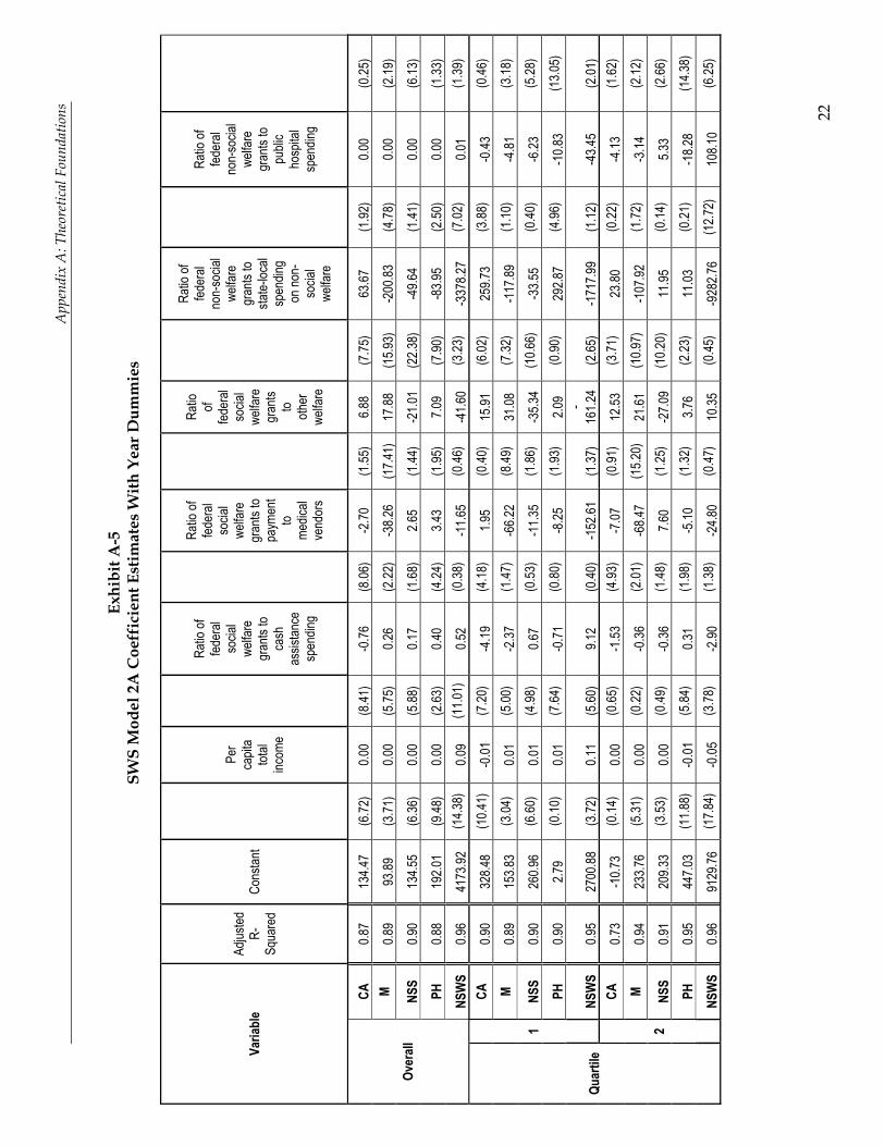
Model 2A Specification
The Model 2 series of models is based on the assumption that grants have price effects but no income effects (i.e., . This is at the other extreme from the Model 1 series of models which assumed that grants have only income effects but no price effects. The type of grant envisioned in the Model 1 series is an unconditional, non-matching grant, e.g., revenue sharing. The type of grant envisioned in the Model 2 series is a block grant restricted to the aided activity with maintenance of effort requirements. Model 2A has no income effects (θo= θs= 0) and has no need variables (λsi= λoi= λyi=0).
Ls + Gs = a1 + b1RL + e1Ms + f1Mo
Lo + Go = a2 + b2RL + e2Ms + f2Mo
Y = a3 + b3RL + e3Ms + f3Mo
The Model 2A estimates are reported in Exhibit A-5.
21
App
endi
x A
: The
oret
ical
Fou
ndat
ions
Exhi
bit A
-5
SWS
Mod
el 2
A C
oeff
icie
nt E
stim
ates
With
Yea
r Dum
mie
s
Varia
ble
Adjus
ted
R-Sq
uare
d Co
nstan
t
Per
capit
a tot
al inc
ome
Ratio
of
feder
al so
cial
welfa
re
gran
ts to
cash
as
sistan
ce
spen
ding
Ratio
of
feder
al so
cial
welfa
re
gran
ts to
paym
ent
to me
dical
vend
ors
Ratio
of
feder
al so
cial
welfa
re
gran
ts to oth
er
welfa
re
Ratio
of
feder
al no
n-so
cial
welfa
re
gran
ts to
state-
local
spen
ding
on no
n-so
cial
welfa
re
Ratio
of
feder
al no
n-so
cial
welfa
re
gran
ts to
publi
c ho
spita
l sp
endin
g
CA
0.87
134.4
7(6
.72)
0.00
(8.41
)-0
.76(8
.06)
-2.70
(1.55
)6.8
8(7
.75)
63.67
(1.92
)0.0
0(0
.25)
M 0.8
9
93
.89(3
.71)
0.00
(5.75
)0.2
6(2
.22)
-38.2
6(1
7.41)
17.88
(15.9
3)-2
00.83
(4.78
)0.0
0(2
.19)
NSS
0.90
134.5
5(6
.36)
0.00
(5.88
)0.1
7(1
.68)
2.65
(1.44
)-2
1.01
(22.3
8)-4
9.64
(1.41
)0.0
0(6
.13)
PH
0.88
192.0
1(9
.48)
0.00
(2.63
)0.4
0(4
.24)
3.43
(1.95
)7.0
9(7
.90)
-83.9
5(2
.50)
0.00
(1.33
)
Over
all
NSW
S 0.9
6
4173
.92(1
4.38)
0.0
9 (1
1.01)
0.5
2 (0
.38)
-11.6
5 (0
.46)
-41.6
0 (3
.23)
-337
8.27
(7.02
) 0.0
1 (1
.39)
CA
0.90
32
8.48
(10.4
1)
-0.01
(7
.20)
-4.19
(4
.18)
1.95
(0.40
) 15
.91
(6.02
) 25
9.73
(3.88
) -0
.43
(0.46
)
M 0.8
9
153.8
3(3
.04)
0.01
(5.00
) -2
.37
(1.47
) -6
6.22
(8.49
) 31
.08
(7.32
) -1
17.89
(1
.10)
-4.81
(3
.18)
NSS
0.90
26
0.96
(6.60
) 0.0
1 (4
.98)
0.67
(0.53
) -1
1.35
(1.86
) -3
5.34
(10.6
6)
-33.5
5 (0
.40)
-6.23
(5
.28)
PH
0.90
2.7
9(0
.10)
0.01
(7.64
) -0
.71
(0.80
) -8
.25
(1.93
) 2.0
9 (0
.90)
292.8
7 (4
.96)
-10.8
3 (1
3.05)
1
NSW
S 0.9
5
27
00.88
(3.72
)0.1
1(5
.60)
9.12
(0.40
)-1
52.61
(1.37
)-
161.2
4(2
.65)
-171
7.99
(1.12
)-4
3.45
(2.01
)CA
0.7
3
-10.7
3(0
.14)
0.00
(0.65
) -1
.53
(4.93
) -7
.07
(0.91
) 12
.53
(3.71
) 23
.80
(0.22
) -4
.13
(1.62
)
M 0.9
4
233.7
6(5
.31)
0.00
(0.22
) -0
.36
(2.01
) -6
8.47
(15.2
0)
21.61
(1
0.97)
-1
07.92
(1
.72)
-3.14
(2
.12)
NSS
0.91
20
9.33
(3.53
) 0.0
0 (0
.49)
-0.36
(1
.48)
7.60
(1.25
) -2
7.09
(10.2
0)
11.95
(0
.14)
5.33
(2.66
)
PH
0.95
44
7.03
(11.8
8)
-0.01
(5
.84)
0.31
(1.98
) -5
.10
(1.32
) 3.7
6 (2
.23)
11.03
(0
.21)
-18.2
8 (1
4.38)
Quar
tile
2
NSW
S 0.9
6
9129
.76(1
7.84)
-0
.05
(3.78
) -2
.90
(1.38
) -2
4.80
(0.47
) 10
.35
(0.45
) -9
282.7
6 (1
2.72)
10
8.10
(6.25
)
22
App
endi
x A
: The
oret
ical
Fou
ndat
ions
Exhi
bit A
-5 (c
ontin
ued)
SW
S M
odel
2A
Coe
ffic
ient
Est
imat
es W
ith Y
ear D
umm
ies
Varia
ble
Adjus
ted
R-Sq
uare
d Co
nstan
t
Per
capit
a tot
al inc
ome
Ratio
of
feder
al so
cial
welfa
re
gran
ts to
cash
as
sistan
ce
spen
ding
Ratio
of
feder
al so
cial
welfa
re
gran
ts to
paym
ent
to me
dical
vend
ors
Ratio
of
feder
al so
cial
welfa
re
gran
ts to oth
er
welfa
re
Ratio
of
feder
al no
n-so
cial
welfa
re
gran
ts to
state-
local
spen
ding
on no
n-so
cial
welfa
re
Ratio
of
feder
al no
n-so
cial
welfa
re
gran
ts to
publi
c ho
spita
l sp
endin
g
M 0.8
9
200.6
9(3
.93)
0.00
(1.86
) -0
.35
(1.85
) -2
4.33
(11.3
6)
3.60
(2.16
) -1
13.51
(1
.42)
0.00
(1.90
)
NSS
0.91
22
8.21
(4.87
) 0.0
0 (0
.60)
0.14
(0.82
) 1.6
8 (0
.86)
-22.7
4 (1
4.83)
36
7.15
(5.01
) 0.0
0 (5
.34)
PH
0.89
-1
46.32
(2.76
) 0.0
0 (2
.28)
0.06
(0.29
) 9.5
1 (4
.27)
5.09
(2.93
) 10
3.12
(1.24
) 0.0
0 (1
.60)
3
NSW
S 0.9
6
3118
.14(9
.20)
0.07
(5.79
) 1.4
9 (1
.20)
-12.6
2 (0
.89)
-13.9
1 (1
.25)
-219
8.79
(4.15
) 0.0
1 (2
.58)
CA
0.51
12
8.56
(3.45
) 0.0
0 (1
.35)
-0.69
(8
.11)
-5.08
(1
.23)
4.66
(4.96
) -1
79.56
(2
.72)
-0.26
(0
.16)
M 0.9
2
121.3
4(2
.25)
0.01
(2.16
) 0.5
3 (4
.26)
-75.4
2 (1
2.60)
19
.46
(14.2
8)
-4.66
(0
.05)
0.12
(0.05
)
NSS
0.91
18
5.22
(6.50
) 0.0
0 (0
.49)
0.10
(1.48
) 8.3
4 (2
.64)
-12.8
0 (1
7.78)
-1
03.67
(2
.05)
1.30
(1.05
)
PH
0.96
-1
42.22
(3.93
) 0.0
1 (6
.40)
0.23
(2.81
) 5.0
4 (1
.25)
4.31
(4.71
) 28
2.63
(4.40
) -1
8.27
(11.5
9)
Quar
tile
4
NSW
S 0.9
5
2949
.56(7
.12)
0.05
(2.97
) 0.3
8 (0
.41)
-81.9
4 (1
.78)
-1.66
(0
.16)
-323
3.69
(4.40
) 31
.09
(1.73
)
CA m
eans
Cas
h Ass
istan
ce, M
mea
ns M
edica
id, N
SS m
eans
Non
-hea
lth S
ocial
Ser
vices
, PH
mean
s Pub
lic H
ospit
al Sp
endin
g, an
d NSW
S me
ans N
on-S
ocial
Welf
are S
pend
ing.
23
Appendix A: Theoretical Foundations
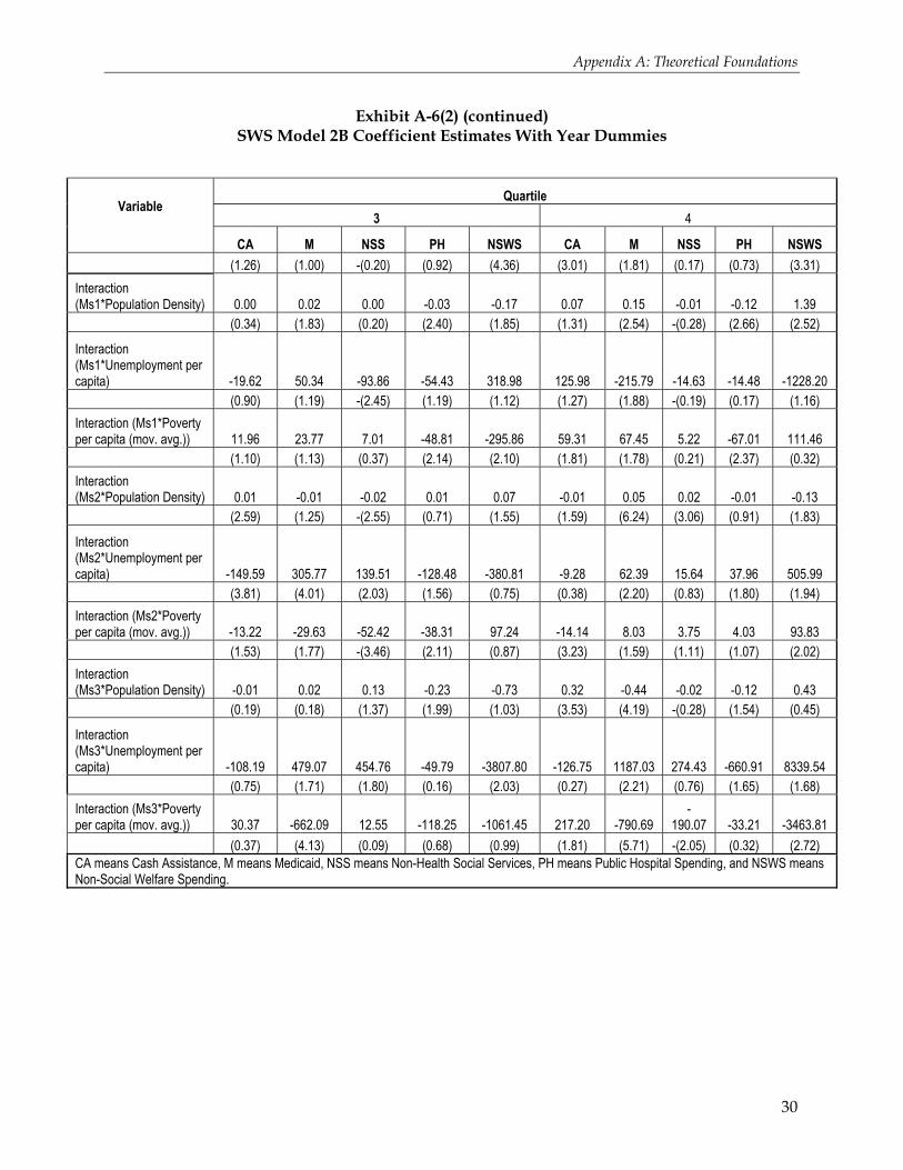
Model 2B Specification
Model 2B is the same as model 2A except that Model 2B includes need variables and their interactions.
Ls + Gs = a1 + b1RL + e1Ms + f1Mo + Σ g1iXi + Σ h1iXi Ms + Σ φ1iXi Mo
Lo + Go = a2 + b2RL + e2Ms + f2Mo + Σ g2iXi + Σ h2iXi Ms + Σ φ2iXi Mo
Y = a3 + b3RL + e3Ms + f3Mo + Σ g3iXi + Σ h3iXi Ms + Σ φ3iXi Mo
The estimates are reported in Exhibit A-6.
24
Appendix A: Theoretical Foundations
Exhibit A-6 SWS Model 2B Coefficient Estimates With Year Dummies
Per capita total income 0.00 0.00 0.00 0.00 0.10 (3.44) (3.05) (3.12) (2.94) (10.94)
Ratio of federal social welfare grants to cash assistance spending 1.45 -1.54 -0.55 0.25 2.20 (3.90) (3.61) (1.37) (0.70) (0.41)
Ratio of federal social welfare grants to payment to medical vendors -10.85 8.50 -10.51 14.06 -1.90 (1.50) (1.03) (1.34) (1.99) (0.02) Ratio of federal social welfare grants to other welfare 7.93 15.54 -21.27 5.76 -18.55 (8.93) (15.29) (22.16) (6.63) (1.44) Ratio of federal non-social welfare grants to state-local spending on non-social welfare 142.83 -31.21 312.56 54.97 -7658.06 (1.74) (0.33) (3.52) (0.68) (6.42) Ratio of federal non-social welfare grants to public hospital spending 0.55 1.76 -0.27 1.58 -12.63 (0.98) (2.76) (0.44) (2.90) (1.56)
Population Density -0.05 -0.11 -0.05 0.02 1.61 (2.21) (4.43) (2.09) (1.08) (5.14)
(1.78) (1.39) (0.30) (0.84) (0.63) Interaction (Ms3*Poverty per capita (mov. avg.)) -13.26 -318.68 137.30 -130.57 -339.38 (0.23) (4.90) (2.24) (2.35) (0.41) CA means Cash Assistance, M means Medicaid, NSS means Non-Health Social Services, PH means Public Hospital Spending, and NSWS means Non-Social Welfare Spending.
Exhibit A-6(1) SWS Model 2B Coefficient Estimates With Year Dummies
Quartile 1 2
CA M NSS PH NSWS CA M NSS PH NSWS Adjusted R-Squared 0.92 0.95 0.92 0.94 0.97 0.87 0.96 0.93 0.98 0.97 Constant 245.36 297.06 267.43 -66.79 581.60 -272.52 -1.78 68.51 275.08 7669.99 (5.23) (5.16) (4.68) (1.86) (0.62) (3.98) (0.04) (0.99) (7.86) (13.67) Per capita total income 0.00 0.01 0.00 0.01 0.19 0.01 0.00 0.01 0.00 0.02 (4.30) (4.11) (3.77) (8.67) (9.41) (3.32) (2.78) (3.23) (0.29) (0.94)
Ratio of federal social welfare grants to cash assistance spending 9.52 -27.91 -4.69 7.06 27.10 1.28 -0.83 -3.51 -0.56 -25.37 (2.60) (6.20) (1.05) (2.52) (0.37) (0.70) (0.62) (1.90) (0.61) (1.70) Ratio of federal social welfare grants to payment to medical vendors -32.99 -88.02 -39.98 -58.58 -571.13 20.07 -4.92 27.58 19.69 392.17 (1.68) (3.64) (1.67) (3.89) (1.44) (0.79) (0.26) (1.06) (1.51) (1.87)
Ratio of federal social welfare grants to other welfare 13.29 25.74 -33.11 0.04 -108.88 15.36 19.86 -29.60 1.04 -2.88 (5.11) (8.05) (10.44) (0.02) (2.08) (5.98) (10.54) (11.35) (0.79) (0.14)
Variable
26
Appendix A: Theoretical Foundations
Exhibit A-6(1) (continued) SWS Model 2B Coefficient Estimates With Year Dummies
Quartile 1 2 Variable
CA M NSS PH NSWS CA M NSS PH NSWS
Ratio of federal non-social welfare grants to state-local spending on non-social welfare 308.45 492.39 741.77 824.92 7780.91 -354.41 -80.79 -679.99 -656.14 -20616.00 (1.83) (2.38) (3.62) (6.41) (2.30) (1.39) (0.43) (2.63) (5.04) (9.88)
Ratio of federal non-social welfare grants to public hospital spending 4.43 4.67 -8.69 -7.60 -433.83 23.20 -9.50 32.16 -3.92 225.31 (1.37) (1.18) (2.21) (3.08) (6.67) (1.97) (1.10) (2.69) (0.65) (2.33) Population Density -0.04 -0.13 -0.09 -0.07 -1.10 0.45 -0.11 -0.83 -0.13 -0.24 (1.05) (3.02) (2.09) (2.61) (1.61) (3.27) (1.08) (6.00) (1.90) (0.22) Unemployment per capita 3696.10 3579.56 2176.27 -428.94 64903.00 -776.94
(1.39) (3.49) (2.17) (1.92) (0.37) (4.47) (2.41) (0.47) (1.71) (2.04) Interaction (Ms3*Poverty per capita (mov. avg.)) 441.69 835.93 618.51 675.99 3820.93 -915.06 -652.55 -194.62 -71.16 -1732.96 (2.13) (3.29) (2.45) (4.27) (0.92) (3.41) (3.32) (0.72) (0.52) (0.79) CA means Cash Assistance, M means Medicaid, NSS means Non-Health Social Services, PH means Public Hospital Spending, and NSWS means Non-Social Welfare Spending.
28
Appendix A: Theoretical Foundations
Exhibit A-6(2) SWS Model 2B Coefficient Estimates With Year Dummies
Quartile 3 4 Variable
CA M NSS PH NSWS CA M NSS PH NSWS Adjusted R-Squared 0.90 0.92 0.93 0.91 0.97 0.59 0.96 0.92 0.97 0.96 Constant -71.16 147.48 169.92 -8.00 4091.37 3.61 124.61 136.66 -216.54 2217.86 (2.02) (2.16) (2.75) (0.11) (8.95) (0.05) (1.55) (2.55) (3.62) (3.00) Per capita total income 0.00 0.00 0.00 0.00 0.04 0.00 0.01 0.00 0.00 0.06 (1.48) (0.22) (1.40) (0.35) (2.63) (1.96) (2.36) (1.40) (0.61) (2.50)
Ratio of federal social welfare grants to cash assistance spending 1.51 -1.08 4.78 4.22 -11.87 2.32 -5.21 -1.77 -0.92 -16.90 (1.46) (0.54) (2.63) (1.94) (0.88) (2.61) (5.08) -(2.59) (1.21) (1.79)
Ratio of federal social welfare grants to payment to medical vendors -0.01 41.46 -15.57 34.49 226.16 -52.10 45.78 31.93 31.38 123.84 (0.00) (2.47) -(1.03) (1.90) (2.02) (2.87) (2.18) (2.28) (2.00) (0.64)
Ratio of federal social welfare grants to other welfare 4.92 5.99 -20.46 6.16 7.07 7.22 11.06 -15.60 1.51 10.96
(0.37) (4.13) (0.09) (0.68) (0.99) (1.81) (5.71) -(2.05) (0.32) (2.72) CA means Cash Assistance, M means Medicaid, NSS means Non-Health Social Services, PH means Public Hospital Spending, and NSWS means Non-Social Welfare Spending.
30
Appendix A: Theoretical Foundations
Model 3A Specification
The Model 3 series regressions all estimate the θo and θs parameters that determine the price effects of grants. Model 3A includes the estimated θo and θs parameters, but no flypaper effect parameters and no need variables, i.e., (Пos= Пoo= Пss = Пso=0), and (λsi= λoi= λyi=0). The model structure is:
Ls + Gs = a1 + b1RL + c1Go + d1Gs + e1Ms + f1Mo
Lo + Go = a2 + b2RL + c2Go + d2Gs + e2Ms + f2Mo
Y = a3 + b3RL + c3Go + d3Gs + e3Ms + f3Mo
The regression results for Model 3A are reported in Exhibit A-7.
31
Appendix A: Theoretical Foundations
Exhibit A-7 SWS Model 3A Coefficient Estimates With Year Dummies
Overall Variable CA M NSS PH NSWS
Adjusted R-Squared 0.87 0.95 0.93 0.89 0.96
Constant 111.97 -21.84 57.54 159.05 4045.78 (5.57) (1.20) (3.15) (8.00) (14.60) Per capita total income -0.01 0.00 0.00 0.00 0.07 (9.37) (6.04) (4.71) (1.13) (9.58)
Federal grants for non-social welfare 0.04 -0.01 0.05 0.08 1.99
(3.95) (1.45) (4.64) (6.85) (12.71)
Federal grants for social welfare 0.06 0.36 0.22 0.08 -0.06
(5.02) (33.84) (21.20) (7.23) (0.36)
Ratio of federal social welfare grants to cash assistance spending
-0.84 0.06 -0.03 0.26 -1.68
(9.00) (0.68) (0.31) (2.85) (1.30)
Ratio of federal social welfare grants to payment to medical vendors
-3.27 -42.45 0.15 2.65 -5.93
(1.90) (27.34) (0.10) (1.56) (0.25)
Ratio of federal social welfare grants to other welfare
4.21 1.13 -31.45 3.32 -35.65
(4.09) (1.22) (33.62) (3.26) (2.51)
Ratio of federal non-social welfare grants to state-local spending on non-social welfare
-86.33 27.86 -132.55 -348.85 -11281.00
(1.56) (0.56) (2.63) (6.36) (14.75)
Ratio of federal non-social welfare grants to public hospital spending
0.00 0.00 0.00 0.00 0.01
(0.17) (1.64) (6.04) (2.04) (0.89)
CA means Cash Assistance, M means Medicaid, NSS means Non-Health Social Services, PH means Public Hospital Spending, and NSWS means Non-Social Welfare Spending.
32
Appendix A: Theoretical Foundations
Exhibit A-7(1) SWS Model 3A Coefficient Estimates With Year Dummies
Quartile 1 2 Variable
CA M NSS PH NSWS CA M NSS PH NSWS Adjusted R-Squared 0.91 0.95 0.94 0.91 0.96 0.73 0.96 0.94 0.96 0.98
(3.90) (0.44) (16.35) (0.58) (0.36) (2.37) (2.52) (17.45) (2.05) (2.51) Ratio of federal non-social welfare grants to state-local spending on non-social welfare
109.11 -141.20
-876.91
-266.41 -14527.00 -
164.36 76.57 50.43 -404.48 -18236.00
(0.86) (1.06) (6.97) (2.50) (5.21) (1.00) (1.01) (0.48) (5.86) (22.76) Ratio of federal non-social welfare grants to public hospital spending
CA means Cash Assistance, M means Medicaid, NSS means Non-Health Social Services, PH means Public Hospital Spending, and NSWS means Non-Social Welfare Spending.
33
Appendix A: Theoretical Foundations
Exhibit A-7(2) SWS Model 3A Coefficient Estimates With Year Dummies
Quartile 3 4 Variable
CA M NSS PH NSWS CA M NSS PH NSWS Adjusted R-Squared 0.84 0.95 0.95 0.90 0.98 0.54 0.97 0.96 0.96 0.98
CA means Cash Assistance, M means Medicaid, NSS means Non-Health Social Services, PH means Public Hospital Spending, and NSWS means Non-Social Welfare Spending.
34
Appendix A: Theoretical Foundations
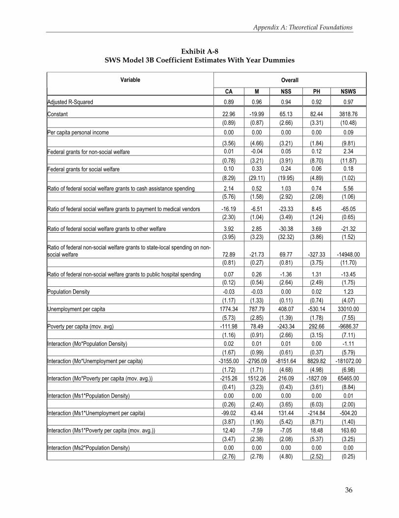
Model 3B Specification
Model 3B adds need variables to the structure of Model 3A. The model structure is the full reduced form:
Ls + Gs = a1 + b1RL + c1Go + d1Gs + e1Ms + f1Mo + Σ g1iXi + Σ h1iXi Ms + Σ φ1iXi Mo
Lo + Go = a2 + b2RL + c2Go + d2Gs + e2Ms + f2Mo + Σ g2iXi + Σ h2iXi Ms + Σ φ2iXi Mo
Y = a3 + b3RL + c3Go + d3Gs + e3Ms + f3Mo + Σ g2iXi + Σ h2iXi Ms + Σ φ2iXi Mo
The results are reported in Exhibit A-8.
35
Appendix A: Theoretical Foundations
Exhibit A-8 SWS Model 3B Coefficient Estimates With Year Dummies
Overall Variable
CA M NSS PH NSWS Adjusted R-Squared 0.89 0.96 0.94 0.92 0.97
Constant 22.96 -19.99 65.13 82.44 3818.76 (0.89) (0.87) (2.66) (3.31) (10.48) Per capita personal income 0.00 0.00 0.00 0.00 0.09
(3.56) (4.66) (3.21) (1.84) (9.81) Federal grants for non-social welfare 0.01 -0.04 0.05 0.12 2.34 (0.78) (3.21) (3.91) (8.70) (11.87) Federal grants for social welfare 0.10 0.33 0.24 0.06 0.18 (8.29) (29.11) (19.95) (4.89) (1.02) Ratio of federal social welfare grants to cash assistance spending 2.14 0.52 1.03 0.74 5.56 (5.76) (1.58) (2.92) (2.08) (1.06)
Ratio of federal social welfare grants to payment to medical vendors -16.19 -6.51 -23.33 8.45 -65.05 (2.30) (1.04) (3.49) (1.24) (0.65)
Ratio of federal social welfare grants to other welfare 3.92 2.85 -30.38 3.69 -21.32 (3.95) (3.23) (32.32) (3.86) (1.52) Ratio of federal non-social welfare grants to state-local spending on non-social welfare 72.89 -21.73 69.77 -327.33 -14948.00 (0.81) (0.27) (0.81) (3.75) (11.70)
CA means Cash Assistance, M means Payments to Medicaid, NSS means Non-Health Social Services, PH means Public Hospital Spending, and NSWS means Non-Social Welfare Spending.
Exhibit A-8(1) SWS Model 3B Coefficient Estimates With Year Dummies
Quartile 1 2 Variable
CA M NSS PH NSWS CA M NSS PH NSWS Adjusted R-Squared 0.94 0.97 0.96 0.95 0.97 0.87 0.98 0.96 0.98 0.99 Constant 137.53 72.54 102.79 -99.75 476.85 -225.43 65.29 56.78 104.03 4010.85 (3.13) (1.71) (2.22) (3.00) (0.51) (2.75) (1.60) (0.92) (2.80) (8.21) Per capita personal income -0.01 0.00 0.00 0.01 0.16 0.01 0.00 0.00 0.00 0.03 (6.03) (4.84) (2.20) (7.38) (8.24) (3.03) (1.98) (2.93) (0.56) (2.35)
Federal grants for non-social welfare 0.03 -0.10 0.09 0.11 2.51 -0.05 -0.09 -0.01 0.18 3.86
Ratio of federal social welfare grants to cash assistance spending 19.22 -10.87 11.18 12.07 85.64 1.34 1.46 0.04 0.76 9.92 (5.56) (3.27) (3.07) (4.62) (1.17) (0.72) (1.58) (0.03) (0.90) (0.89)
Ratio of federal social welfare grants to payment to medical vendors -35.64 -100.29 -41.75 -55.02 -468.60 19.03 -20.95 4.22 13.16 206.47 (2.04) (5.96) (2.26) (4.16) (1.26) (0.74) (1.65) (0.22) (1.14) (1.35)
Ratio of federal social welfare grants to other welfare 2.78 5.14 -49.58 -3.99 -138.94 13.29 4.08 -49.94 -0.55 -77.51 (1.04) (2.01) (17.69) (1.99) (2.46) (4.20) (2.60) (21.10) (0.39) (4.12)
37
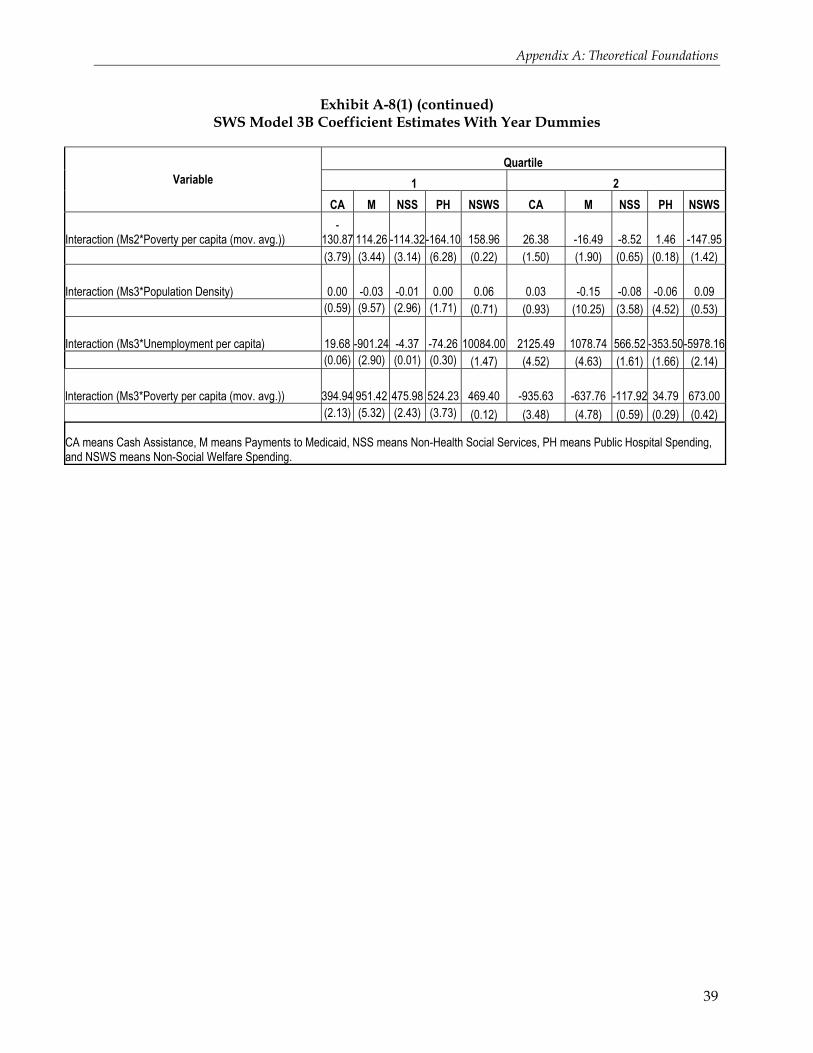
Appendix A: Theoretical Foundations
Exhibit A-8(1) (continued) SWS Model 3B Coefficient Estimates With Year Dummies
Quartile 1 2 Variable
CA M NSS PH NSWS CA M NSS PH NSWS
Ratio of federal non-social welfare grants to state-local spending on non-social welfare -80.54 473.15 -116.54 195.25 -4880.26 -382.01 -77.36 -603.72 -525.57 -17688.00 (0.45) (2.75) (0.62) (1.44) (1.28) (1.49) (0.61) (3.14) (4.53) (11.58) Ratio of federal non-social welfare grants to public hospital spending 3.91 2.89 -9.23 -7.29 -423.17 24.32 -13.95 22.10 -12.24 28.19 (1.36) (1.04) (3.05) (3.36) (6.93) (2.03) (2.35) (2.47) (2.26) (0.40) Population Density -0.02 -0.06 -0.06 -0.08 -1.42 0.52 0.25 -0.45 -0.22 -1.35 (0.50) (2.10) (1.95) (3.28) (2.19) (3.59) (3.43) (4.10) (3.37) (1.56) Unemployment per capita 2888.75 2182.55 848.60 -859.22 59706.00 -858.77 -1177.14 250.51 -899.10 542.35 (4.47) (3.51) (1.25) (1.76) (4.35) (1.07) (2.97) (0.42) (2.49) (0.11) Poverty per capita (mov. avg) -183.02 -1649.62 -53.60 744.23 -3994.31 1409.49 353.36 -489.44 707.80 3684.03 (0.57) (5.33) (0.16) (3.06) (0.58) (3.59) (1.82) (1.67) (3.99) (1.58)
CA means Cash Assistance, M means Payments to Medicaid, NSS means Non-Health Social Services, PH means Public Hospital Spending, and NSWS means Non-Social Welfare Spending.
39
Appendix A: Theoretical Foundations
Exhibit A-8(2) SWS Model 3B Coefficient Estimates With Year Dummies
Quartile 3 4 Variable
CA M NSS PH NSWS CA M NSS PH NSWS Adjusted R-Squared 0.93 0.97 0.96 0.92 0.99 0.59 0.98 0.96 0.97 0.99 Constant -140.04 -46.57 21.12 -90.43 3969.83 14.45 66.57 93.73 -200.84 2718.54 (4.58) (1.07) (0.44) (1.26) (11.89) (0.21) (1.28) (2.53) (3.39) (7.42) Per capita personal income 0.00 0.00 0.00 0.00 0.03 0.00 0.01 0.00 0.00 0.00 (1.38) (0.24) (1.37) (0.12) (3.07) (1.97) (2.85) (1.83) (0.36) (0.17) Federal grants for non-social welfare 0.03 -0.02 0.06 0.14 4.05 0.01 0.10 0.01 0.05 5.54 (1.47) (0.47) (1.71) (2.46) (15.81) (0.28) (3.44) (0.48) (1.35) (26.86) Federal grants for social welfare 0.13 0.37 0.28 0.15 -0.03 -0.05 0.33 0.21 -0.05 0.19 (10.02) (20.27) (13.90) (4.89) (0.23) (1.91) (17.77) (16.11) (2.59) (1.50) Ratio of federal social welfare grants to cash assistance spending 2.20 0.81 6.27 5.09 -8.75 1.77 -1.05 0.82 -1.50 -4.00 (2.50) (0.64) (4.55) (2.45) (0.91) (1.89) (1.50) (1.64) (1.88) (0.81) Ratio of federal social welfare grants to payment to medical vendors -0.74 48.30 -16.22 26.16 -90.26 -40.95 -31.59 -18.15 44.29 80.05 (0.10) (4.51) (1.38) (1.47) (1.10) (2.16) (2.22) (1.79) (2.73) (0.80) Ratio of federal social welfare grants to other welfare 3.04 0.45 -24.55 4.10 11.86 8.62 1.68 -21.77 3.18 15.47 (4.16) (0.44) (21.52) (2.38) (1.49) (6.30) (1.65) (29.80) (2.73) (2.14) Ratio of federal non-social welfare grants to state-local spending on non-social welfare 191.12 -459.57 251.14 -1310.35 -18502.00 607.85 -357.08
-155.15 174.23
-24736.00
(1.28) (2.16) (1.07) (3.72) (11.32) (2.50) (1.96) (1.19) (0.84) (19.28) Ratio of federal non-social welfare grants to public hospital spending -1.36 -3.34 0.70 6.92 -5.30 -14.04 -4.24 3.58 -3.70 46.64 (1.00) (1.73) (0.33) (2.16) (0.36) (3.22) (1.30) (1.54) (0.99) (2.03) Population Density 0.59 0.43 -0.37 0.15 -0.91 0.93 -0.43 0.01 2.62 8.78 (3.79) (1.93) (1.52) (0.40) (0.54) (2.54) (1.57) (0.06) (8.40) (4.57)
CA means Cash Assistance, M means Payments to Medicaid, NSS means Non-Health Social Services, PH means Public Hospital Spending, and NSWS means Non-Social Welfare Spending.