Page 1
Sphere Intersection 3D Shape Descriptor (SID)
Author1a,∗, Author2a, Author3a
aSome Affiliation, Country
Abstract
This paper presents a novel 3D shape descriptor which explicitly captures the
local geometry and encodes it using an efficient representation. Our method
consists of multiple evolving fronts which are realized by a set of growing spheres
on the surface. At the core of this method is a simple intersection operator
between the spheres and the shape’s surface. Intersection curves yield a discrete
sampling of the surface at different positions and scales. Our key idea is to define
a shape descriptor that captures the continuous local geometry of the surface
in an efficient and consistent representation by intersecting the surface with
multiple spheres and transforming the intersection curve to frequency domain.
To evaluate our descriptor, we define shape similarity metric and perform shape
matching on the SHREC11 non-rigid benchmark and other classes.
Keywords: mesh processing, descriptor, signature, similarity, retrieval
1. Introduction
Databases of 3D models are becoming nowadays available in a number of
disciplines, including computer graphics, CAD, and medicine [1]. As a result of
the extensive growth of 3D databases, shape-retrieval techniques are becoming
valuable tools for analysis and discovery. The SHREC contest and benchmark [2]
have been stimulating forces in this field.
∗Corresponding authorEmail address: [email protected] (Author1)
1+972558836169
Preprint submitted to Computer Aided Geometric Design August 30, 2015
Page 2
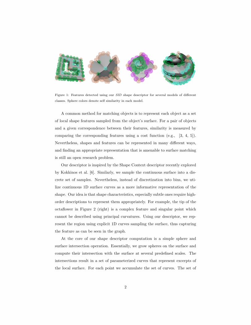
Figure 1: Features detected using our SID shape descriptor for several models of different
classes. Sphere colors denote self similarity in each model.
A common method for matching objects is to represent each object as a set
of local shape features sampled from the object’s surface. For a pair of objects
and a given correspondence between their features, similarity is measured by
comparing the corresponding features using a cost function (e.g., [3, 4, 5]).
Nevertheless, shapes and features can be represented in many different ways,
and finding an appropriate representation that is amenable to surface matching
is still an open research problem.
Our descriptor is inspired by the Shape Context descriptor recently explored
by Kokkinos et al. [6]. Similarly, we sample the continuous surface into a dis-
crete set of samples. Nevertheless, instead of discretization into bins, we uti-
lize continuous 1D surface curves as a more informative representation of the
shape. Our idea is that shape characteristics, especially subtle ones require high-
order descriptions to represent them appropriately. For example, the tip of the
octaflower in Figure 2 (right) is a complex feature and singular point which
cannot be described using principal curvatures. Using our descriptor, we rep-
resent the region using explicit 1D curves sampling the surface, thus capturing
the feature as can be seen in the graph.
At the core of our shape descriptor computation is a simple sphere and
surface intersection operation. Essentially, we grow spheres on the surface and
compute their intersection with the surface at several predefined scales. The
intersections result in a set of parameterized curves that represent excerpts of
the local surface. For each point we accumulate the set of curves. The set of
2
Page 3
curves is then transformed to the frequency domain, resulting in a compact yet
effective 2D representation of local 3D geometry.
We define a shape similarity metric based on the correlation between ”in-
teresting shape features” and curvature, following the observation of Marr [7].
To compare two shapes, we filter out smooth or flat regions, and compare the
curved regions by measuring the distance between their descriptors.
We evaluate our work by performing both qualitative and quantitative anal-
ysis. For qualitative evaluation we use multiple shapes with different character-
istics and deformations (see Figures 2, 8 and 1). For quantitative evaluation
we use the SHREC 11 non-rigid benchmark [2] and SHREC 12 abstract shapes
benchmark [8]. The results show that SID outperforms most state-of-the-art
algorithms used in the comparison in terms of retrieval rates. With regards to
MeshSIFT [9], although retrieval rates are similar to us, we observe that SID
holds favorable properties in terms of speed, meaningful keypoint selection and
consistency of keypoint selection.
Our contributions are as follows:
• A descriptor which captures the shape via explicit sampling of the surface
with continuous 1D curves at keypoints. Our descriptor is informative and
distinctive (see Figure 2).
• An efficient and meaningful feature detection scheme based on our de-
scriptor formulation.
• A shape retrieval scheme which offers a unique balance and combination
of correctness, speed and handling multiple classes of shapes.
2. Related Work
Shape descriptors and similarity have been extensively studied in fields such
as computer-vision, CAD and molecular-biology [1]. In 2D images and video,
shape matching has been broadly researched [10, 11, 12, 13] and is beyond
the scope of this work. A major problem in extending these systems to 3D
3
Page 4
Figure 2: Two shapes with complex features (knot-left, octaflower-right), such as curvature
extrema, saddle and singular points. For each green sphere on shapes, graphs to the right
show the parameterized intersection curve. Note the large differences in the graphs between
the saddle point (left) and singular tip point (right).
is that 3D models typically lack an underlying regular parametric domain. For
example, 2D shapes have a natural arc length parametrization of their boundary
contours while 3D surfaces of arbitrary genus do not. As a result, common shape
descriptors for 2D contours (e.g., [14, 15, 16]) cannot be directly extended to
3D surfaces.
Nevertheless, descriptors for 3D shape matching have been studied for more
than two decades. Gaussian images [17] and spherical representations [18] are
global representations useful for describing simple objects. Stein and Medioni [19]
recognize 3D objects by matching points using structural indexing and their
”splash” representation. Similarly, Chua and Jarvis match points to align sur-
faces using principal curvatures [20] and ”point-signatures” [4]. The Harmonic
shape images [21] map a patch that is topologically equivalent to a disk into
a 2D domain. Similar to this work, Spin Images [5] encode the local patch
geometry in a compact 2D image using cylindrical coordinates.
Our descriptor significantly differs from these methods as it encodes contin-
uous surface excerpts around a point. Thus, instead of analyzing local proper-
ties (for example curvature), we capture the actual surface by encoding curves
around a point. This representation benefits from both being compact and
yet descriptive. Nonetheless, our formulation is simple, requiring only to com-
pute a surface intersection with a sphere and is not restricted to disk-like patch
topology.
4
Page 5
Another approach for describing shapes is indexing their features based
on statistical properties. Histograms of geometric statistics have been consid-
ered [22, 23, 24] as well as harmonic-based representations [25, 26]. Ankerst et
al. [22] propose global histograms encoding shells and sectors around a model’s
centroid. Osada et al. [23] represent shapes with probability distributions of ge-
ometric properties computed from random points. Kazhdan et al. [26] represent
the global shape using spherical harmonics, for rotational invariant descriptors.
Giorgi et al [27] utilize best view selection to generate descriptive 2D binary
images from 3D models for effective matching. While these methods propose
alternate surface representations, ours encodes the explicit surface. Hence, it
retains all surface properties and characteristics.
Multi-scale features similar to 2D SIFT [28] have been explored in the context
of 3D shapes [29, 30, 9]. These techniques develop local shape descriptors based
on differential properties and scalar functions of the mesh surface. MeshSIFT [9]
detects features by smoothing the mesh at various degrees and seeking for local
minima/maxima of mean curvature. The feature description is performed by
constructing a histogram of slant and angle per each scale in scale space.
Zaharescu et al. [30] present MeshHOG which seeks Laplacian extrema in
a scalar function defined on a surface. Sun et al. [31] and Kokkinos et al. [32]
utilize heat-kernels to compute the bending invariant shape signatures. The use
of heat-kernels has many benefits such as mathematically provable properties
and detection of small number of meaningful features but is also time consuming
and implicit representations of the surface. Pottmann et al. [33] analyze the
stability of differential properties on surfaces with regard to their scale. Sipiran
et al. [34] extend the 2D Harris operator to 3D meshes, they analyze the k-ring
of vertices around a point in order to form the descriptor and propose two modes
of operation for feature detection: choosing points with highest Harris value or
clustering. The first method suffers from choosing multiple features on sharp
edges of the surface thus being somewhat ambiguous in the feature selection
result. The second method suffers from lesser repeatability according to the
authors. Darom et al. [35] show scale invariant extensions of the SIFT and
5
Page 6
Spin Images descriptors to 3D meshes. Similar to these works, we also define
our shape descriptor in a scale-space context. Nevertheless, our signature is an
explicit representation of the surface and not an implicit measurement of a scalar
function, shape distribution or differential properties. Thus, our representation
is less sensitive to noise and surface inconsistencies.
In a seminal work, Tombari et al. [36] evaluated and compared 3D feature
descriptors. A major conclusion was that the number of keypoints do not cor-
relate with matching success. For example, KPQ [37] finds many keypoints and
yields good matching scores in contrast to HKS[31] and Salient Points[38] which
both find very few keypoints and both sub-performed. We come to the conclu-
sion that detecting a small number of meaningful features that produce good
retrieval results is still a major challenge. Our method specifically addresses
this challenge.
Mortara et al. [39] explore different characteristics of intersection curve re-
sulting from intersecting a sphere with a triangle mesh. Some of the charac-
teristics considered are: concavity vs. convexity, curve length and number of
connected components. Their research focused on segmentation of shapes rather
than shape retrieval, and did not address the question of fine grain dissimilarity
between features. We choose to further explore the sphere to mesh intersection
curve with respect to mesh retrieval application.
3. Overview
Our framework consists of the following main components: feature detection,
feature description, shape similarity. In the following we provide an overview of
each component.
• Feature detection: the selection of features is done iteratively with
spheres of growing radius, centered at mesh vertices. At each step of
the feature detection loop we compute a saliency metric on the sphere
intersection curve with the surface. Intersecting spheres are detected and
6
Page 7
Figure 3: Sphere Intersection Descriptor (SID) of a single feature overview. Upper left: two
sphere intersections with different radii. Bottom left: corresponding parameterized intersec-
tion curves. Upper right: multiple intersections aggregated. Bottom right: frequency domain
transformation yielding a compact 2D image representation.
only spheres with stronger metric are kept for the next iteration. Figure
6 demonstrates the iterative detection process.
• Feature Description: given a keypoint and a support sphere radius
from the previous step, the sphere intersection curve with the surface is
projected to spherical coordinates and parameterized to φ(t), θ(t) compo-
nents. Lastly, φ(t), θ(t) are transformed to frequency domain thus produc-
ing rotational invariant local feature descriptor. Figure 3 demonstrates the
sphere intersection with the mesh, the resulting curve on the (φ, θ) plane
and the transformation to frequency domain.
• Shape Similarity: for similarity computation between two meshes, we
perform a min cost maximal matching on a bipartite graph generated from
the set of descriptors of each mesh. Similarity between two given feature
descriptors is given by L1 distance of their magnitudes. Thus, model
correspondence is performed by minimizing the cost of the matching on
the feature descriptors sets.
7
Page 8
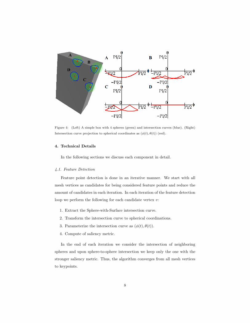
Figure 4: (Left) A simple box with 4 spheres (green) and intersection curves (blue). (Right)
Intersection curve projection to spherical coordinates as (φ(t), θ(t)) (red).
4. Technical Details
In the following sections we discuss each component in detail.
4.1. Feature Detection
Feature point detection is done in an iterative manner. We start with all
mesh vertices as candidates for being considered feature points and reduce the
amount of candidates in each iteration. In each iteration of the feature detection
loop we perform the following for each candidate vertex v:
1. Extract the Sphere-with-Surface intersection curve.
2. Transform the intersection curve to spherical coordinations.
3. Parameterize the intersection curve as (φ(t), θ(t)).
4. Compute of saliency metric.
In the end of each iteration we consider the intersection of neighboring
spheres and upon sphere-to-sphere intersection we keep only the one with the
stronger saliency metric. Thus, the algorithm converges from all mesh vertices
to keypoints.
8
Page 9
4.1.1. Sphere Intersection Curve
Given a vertex v and radius r we compute the intersection of a sphere of
radius r centered at v with the mesh surface. This gives a closed loop of adjacent
faces that intersect with the sphere. By choosing the initial radius to be small
enough, we enforce only one closed loop per sphere in the first iteration. Then,
each iteration we increase r and compute a new sphere intersection curve. In case
that the sphere intersection produces several closed loops of faces we take the
faces loop closest to the loop from the previous iteration. it follows by induction
that we always have one closed loop and that it will not jitter between different
components.
Figure 5: Sphere intersection illustration showing the triangle intersection with arc and its
sampling.
The faces are sampled uniformly so we obtain the intersection curve points
in global Euclidean coordinate system (see Figure 5). Then we impose a local
Euclidean coordinate system UVW , with origin at v and its W axis as the
consistent normal at v. We arbitrarily set the UV axes to be orthonormal to
W .
9
Page 10
The consistent normal of v is computed as follows:
cn(v) =
normal(v) ,if ‖v − icc‖ < t
sign((v − icc) · normal(v)) · v−icc‖v−icc‖ ,else
(1)
where icc is the intersection curve centroid and t is a threshold. The first case
sets the consistent normal of v to be the normal of v if the intersection curve
centroid is too close to v (determined by threshold t). The purpose of this case
is to prevent ”jitter” of the consistent normal at small scales. The second case
sets the consistent normal of v to be the vector connecting the intersection curve
centroid and v, we enforce the consistent normal to be in the same direction
of the original normal of v by multiplying with sign((v − icc) · normal(v)).
The construction of the consistent normal follows the direction of the original
normal and gives a normal that is invariant to different deformations: non rigid,
local noise and various triangulations. Thus, we obtain a stable local coordinate
system for locally similar surfaces.
Next follows the transformation of c points to local spherical coordinate sys-
tem. Since r is constant, we can represent c as two 1D functions defined by
(θ, φ) , where φ, θ ∈ [−π/2, ..., π/2]. We parameterize the intersection curve
by performing a walk on the curve c and encoding the angles (θ, φ) with re-
spect to the axes. The intersection curve points are transformed into spherical
coordinates following the formula:
φ = sin(atan2(px, py)) (2)
θ = asin(pz) (3)
Where (px, py, pz) is a point on c in local Euclidean coordinate system. We
apply a sin function to φ as we require a cyclic function for the fourier trans-
form. The origin of φ (i.e., φ = 0) is determined by the rotational orientation
of the spherical coordinate system imposed at p. See Figures 4 and 3 for
demonstration of this operation.
10
Page 11
4.1.2. Sphere-to-Sphere Intersection
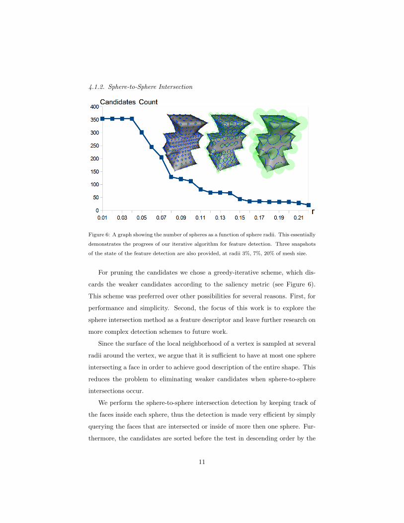
Figure 6: A graph showing the number of spheres as a function of sphere radii. This essentially
demonstrates the progrees of our iterative algorithm for feature detection. Three snapshots
of the state of the feature detection are also provided, at radii 3%, 7%, 20% of mesh size.
For pruning the candidates we chose a greedy-iterative scheme, which dis-
cards the weaker candidates according to the saliency metric (see Figure 6).
This scheme was preferred over other possibilities for several reasons. First, for
performance and simplicity. Second, the focus of this work is to explore the
sphere intersection method as a feature descriptor and leave further research on
more complex detection schemes to future work.
Since the surface of the local neighborhood of a vertex is sampled at several
radii around the vertex, we argue that it is sufficient to have at most one sphere
intersecting a face in order to achieve good description of the entire shape. This
reduces the problem to eliminating weaker candidates when sphere-to-sphere
intersections occur.
We perform the sphere-to-sphere intersection detection by keeping track of
the faces inside each sphere, thus the detection is made very efficient by simply
querying the faces that are intersected or inside of more then one sphere. Fur-
thermore, the candidates are sorted before the test in descending order by the
11
Page 12
saliency metric, this ensures that no candidate is unnecessarily eliminated.
4.1.3. Saliency Metric
We follow the observation of Marr [7] which correlates between ”interesting
shape features” and surface sharpness. We define interesting points as points
having non-smooth or flat curvature. The detection of feature points is crucial:
important parts of the objects should not be missed, while the overall number
of feature points directly affects the computational complexity and introduces
unimportant information.
Since our feature is an intersection curve along the mesh surface, many for-
mulations can be considered as sole saliency metric or as a combined weighted
sum - integral, Laplacian and variance just to name a few. For our imple-
mentation we chose to use a weighted sum of integral of absolute value of the
intersection curve and sum of Laplacians. Given a vertex v let θv(t), φv(t) be
defined for t ∈ 1, ..., n then the sum of Laplacians of v is defined by:
lv =∑ ∂2θv
∂t2(4)
and integral of absolute value of the intersection curve of v is defined by:
iv =
n−1∑t=1
∥∥∥∥ (θv(t+ 1)− θv(t)) · (φv(t+ 1) + φv(t))
2
∥∥∥∥ (5)
then the saliency metric is given by a normalized weighted sum of lv and iv.
This formulation gives high saliency values both to features at local ex-
trema/minima and also to features with great variation in their local neighbor-
hood. In Figure 2 the left feature is considered strong because of its sum of
Laplacians value while the feature on the right is considered strong because of
high integral of absolute value of the intersection curve value.
In our implementation we set n = 128 and Laplacian aperture size to be
15. The weight of the components varies according to input characteristics.
For example, for meshes of living creatures with limbs and edges of varying
properties (see Figure 12) only integral of absolute value of the intersection
curve was used. Alternatively, for simple geometric meshes a weighted sum of
12
Page 13
integral of absolute value of the intersection curve and sum of Laplacians was
used (see Figure 1 and Figure 11).
4.2. Feature Description
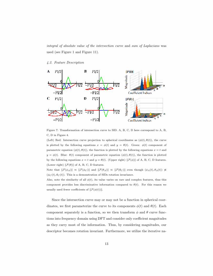
Figure 7: Transformation of intersection curve to SID. A, B, C, D here correspond to A, B,
C, D in Figure 4.
(Left) Red: Intersection curve projection to spherical coordinates as (φ(t), θ(t)), the curve
is plotted by the following equations x = φ(t) and y = θ(t). Green: φ(t) component of
parametric equation (φ(t), θ(t)), the function is plotted by the following equations x = t and
y = φ(t). Blue: θ(t) component of parametric equation (φ(t), θ(t)), the function is plotted
by the following equations x = t and y = θ(t). (Upper right) ‖F(φ)‖ of A, B, C, D features.
(Lower right) ‖F(θ)‖ of A, B, C, D features.
Note that ‖F(φA)‖ ≈ ‖F(φC)‖ and ‖F(θA)‖ ≈ ‖F(θC)‖ even though (φA(t), θA(t)) 6≈
(φC(t), θC(t)). This is a demonstration of SIDs rotation invariance.
Also, note the similarity of all φ(t), its value varies on rare and complex features, thus this
component provides less discriminative information compared to θ(t). For this reason we
usually used fewer coefficients of ‖F(φ(t))‖.
Since the intersection curve may or may not be a function in spherical coor-
dinates, we first parameterize the curve to its components φ(t) and θ(t). Each
component separately is a function, so we then transform φ and θ curve func-
tions into frequency domain using DFT and consider only coefficient magnitudes
as they carry most of the information. Thus, by considering magnitudes, our
descriptor becomes rotation invariant. Furthermore, we utilize the iterative na-
13
Page 14
ture of the feature detection phase to consider this formulation at multiple scales
[r1 − rmax] thus providing a discrete sampling of co-centric intersection curves
around a keypoint (see Figure 3).
For a given vertex v we consider the following as a feature descriptor:
SID(vi) = ‖F(φr1v )‖ , ‖F(θr1v )‖ , · · · , ‖F(φrmaxv )‖ , ‖F(θrmax
v )‖ (6)
This descriptor is computed for each keypoint detected in the feature detec-
tion phase.
An additional advantage of using Fourier Transform is the control it gives
us on the desired level of detail. We can take few coefficients from the result
of the DFT to favor compactness or many coefficients to favor descriptiveness.
We empirically chose to take more ‖F(θ)‖ coefficients since it carries more
information then ‖F(φ)‖.
4.2.1. Rotation Invariance
In order to underline and clarify the rotation invariance of our descriptor we
provide the following elaboration using both a figure and a formal discussion.
Figure 4 and Figure 7 demonstrate the rotational invariance. Features A and
C in Figure 4 are both similar in shape since they are both on a straight angle
edge, but those features differ in rotation and in phase. The phase difference is
observable in Figure 4 in the graphs of A and C. Despite the rotation and phase
shift between A and C, Figure 7 clearly shows the final descriptor is similar
(‖F(φA)‖ ≈ ‖F(φC)‖ and ‖F(θA)‖ ≈ ‖F(θC)‖) both in the φ (Figure 7, upper
right, A and C rows) and θ (Figure 7, upper right, A and C rows) components.
For the general case, consider a surface S1, a point v1 on S1, a surface
S2 = R(S1) where R is rotational transformation and a point v2 = R(v1), notice
that v2 is on S2. For a given radius r we set a sphere around v1 and set another
sphere with radius r around v2. Next, let i1 be the intersection curve of the
first sphere with S1, and correspondingly let i2 be the intersection curve of the
second sphere with S2. The consistent normal (see Section 4.1.1 for definition)
W1 is the vector between v1 and the centroid of i1, W2 is constructed similarly
14
Page 15
using v2 and i2. Notice that W2 = R(W1). Next, U1V1 are the arbitrary,
orthonormal axes to W1 axis. U2V2 are the equivalent with respect to W2.
Denote φ1 and θ1 as i1 transformed to spherical coordinates and broken down to
components according to the U1V1W1 coordinate system. Denote φ2 and θ2 as i2
transformed to spherical coordinates and broken down to components according
to the U2V2W2 coordinate system. Since W2 = R(W1), we get similar but phase
shifted functions: φ1(t) = φ2(t − δ1), θ1(t) = θ2(t − δ2). Performing DFT on
each component: φ1, φ2, θ1, θ2 and keeping only the magnitudes component
eliminates exactly the phase shift. ‖F(φ1)‖ = ‖F(φ2)‖, ‖F(θ1)‖ = ‖F(θ2)‖.
Thus, using ‖F(φ)‖ and ‖F(θ)‖ as feature descriptors makes invariant feature
descriptor.
4.3. Shape Similarity
We reduce shape similarity problem to the problem of finding a minimal
cost matching in a bipartite graph. Given two shapes ma, mb and Fa, Fb are
their detected features, we define the bipartite graph as the two sets (Fa, Fb),
whereas edge costs are computed by the L1 distance of the magnitudes vector
of features. The resulting minimal cost matching gives the best possible pairing
of features, thus providing accurate similarity metric for shape matching.
5. Results and Details
Our implementation is written in C++ using OpenMesh [41], OpenCV [42]
and LEMON [43] for min cost bipartite graph matching. We make our source
code available for public to encourage experimentation and further exploration
of the SID shape descriptor. http://sourceforge.net/projects/sphere-intersection-
signature/
We have tested our implementation on various polygonal models. Figures
1, 8 and 9 present a qualitative demonstration of our descriptor effectiveness
where similar features are accurately matched together (i.e. colored by the same
color).
15
Page 16
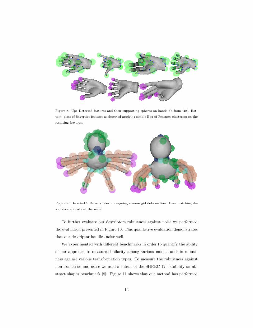
Figure 8: Up: Detected features and their supporting spheres on hands db from [40]. Bot-
tom: class of fingertips features as detected applying simple Bag-of-Features clustering on the
resulting features.
Figure 9: Detected SIDs on spider undergoing a non-rigid deformation. Here matching de-
scriptors are colored the same.
To further evaluate our descriptors robustness against noise we performed
the evaluation presented in Figure 10. This qualitative evaluation demonstrates
that our descriptor handles noise well.
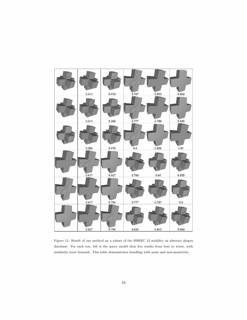
We experimented with different benchmarks in order to quantify the ability
of our approach to measure similarity among various models and its robust-
ness against various transformation types. To measure the robustness against
non-isometries and noise we used a subset of the SHREC 12 - stability on ab-
stract shapes benchmark [8]. Figure 11 shows that our method has performed
16
Page 17
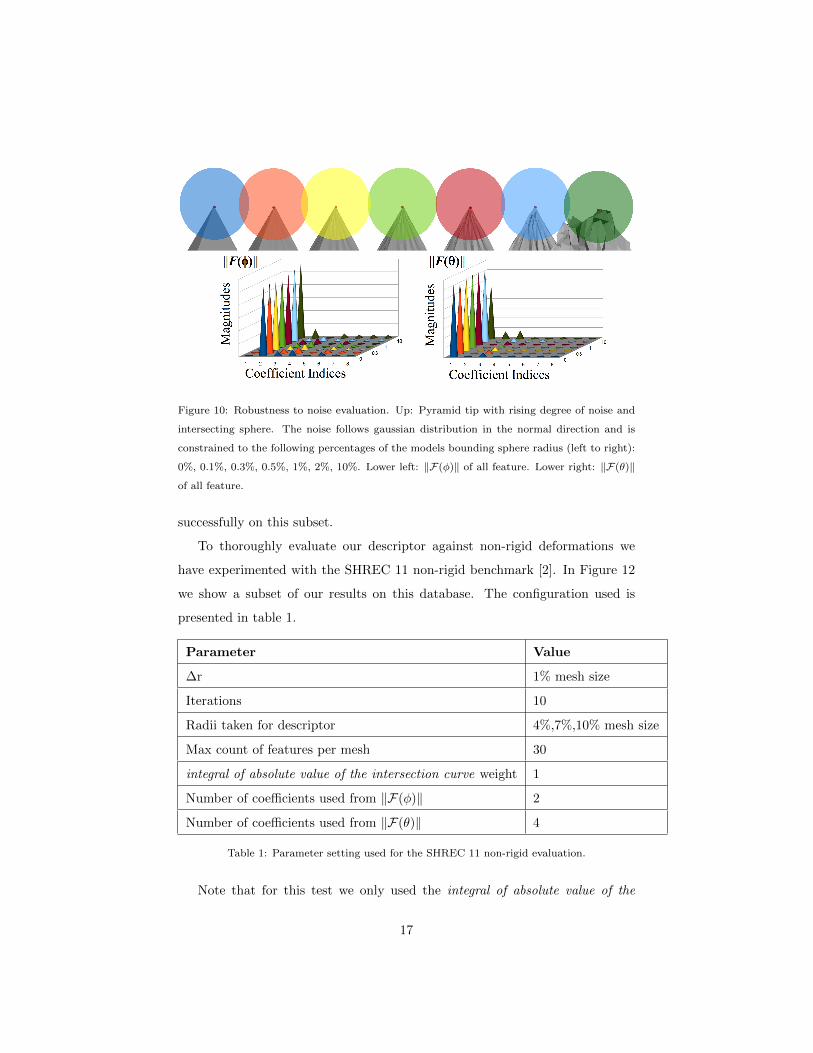
Figure 10: Robustness to noise evaluation. Up: Pyramid tip with rising degree of noise and
intersecting sphere. The noise follows gaussian distribution in the normal direction and is
constrained to the following percentages of the models bounding sphere radius (left to right):
0%, 0.1%, 0.3%, 0.5%, 1%, 2%, 10%. Lower left: ‖F(φ)‖ of all feature. Lower right: ‖F(θ)‖
of all feature.
successfully on this subset.
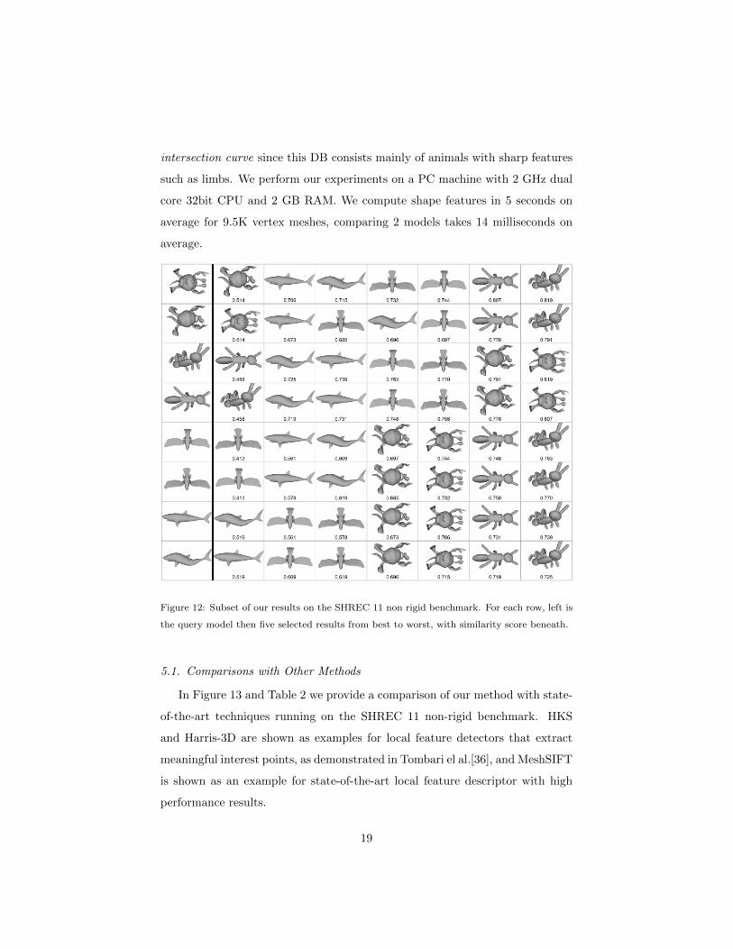
To thoroughly evaluate our descriptor against non-rigid deformations we
have experimented with the SHREC 11 non-rigid benchmark [2]. In Figure 12
we show a subset of our results on this database. The configuration used is
presented in table 1.
Parameter Value
∆r 1% mesh size
Iterations 10
Radii taken for descriptor 4%,7%,10% mesh size
Max count of features per mesh 30
integral of absolute value of the intersection curve weight 1
Number of coefficients used from ‖F(φ)‖ 2
Number of coefficients used from ‖F(θ)‖ 4
Table 1: Parameter setting used for the SHREC 11 non-rigid evaluation.
Note that for this test we only used the integral of absolute value of the
17
Page 18
Figure 11: Result of our method on a subset of the SHREC 12 stability on abstract shapes
database. For each row, left is the query model then five results from best to worst, with
similarity score beneath. This table demonstrates handling with noise and non-isometries.
18
Page 19
intersection curve since this DB consists mainly of animals with sharp features
such as limbs. We perform our experiments on a PC machine with 2 GHz dual
core 32bit CPU and 2 GB RAM. We compute shape features in 5 seconds on
average for 9.5K vertex meshes, comparing 2 models takes 14 milliseconds on
average.
Figure 12: Subset of our results on the SHREC 11 non rigid benchmark. For each row, left is
the query model then five selected results from best to worst, with similarity score beneath.
5.1. Comparisons with Other Methods
In Figure 13 and Table 2 we provide a comparison of our method with state-
of-the-art techniques running on the SHREC 11 non-rigid benchmark. HKS
and Harris-3D are shown as examples for local feature detectors that extract
meaningful interest points, as demonstrated in Tombari el al.[36], and MeshSIFT
is shown as an example for state-of-the-art local feature descriptor with high
performance results.
19
Page 20
Method NN FT ST E DCG
SID (Our) 0.973 0.767 0.878 0.638 0.934
HKS 0.837 0.406 0.497 0.353 0.730
3D-Harris 0.562 0.325 0.466 0.322 0.654
MeshSIFT 0.995 0.884 0.962 0.708 0.980
Table 2: Performance evaluation on SHREC 11 - non rigid. Nearest Neighbor (NN), First
Tier (FT), Second Tier (ST), E-measure (E), and Discounted Cumulative Gain (DCG). See
PSB [44] for full definition of the measures.
Figure 13: Precision-recall graph on the SHREC11-non-rigid benchmark. See PSB [44] for
full definition of the precision-recall measure.
20
Page 21
We discuss our comparison with respect to each method in detail:
Harris3D [34]. In SHREC11 [2] the authors of Harris3D chose to use a geodesic
map scheme. After detecting interest points by the Harris3D method, a geodesic
map is constructed by considering normalized geodesic distances between all
pairs of interest points. In contrast to considering mere scalar distances between
keypoints, SID considers the geometry of the features themselves. We attribute
the superiority of SID on Harris3D to the usage of fine feature geometry rather
then distances.
HKS [31] based Point-to-point Matching. HKS uses a descriptor comprised of
samples along the continuous representation of the Heat Kernel Signature. SID
also uses discrete sampling of functions (φ(t), θ(t)), but it compacts the descrip-
tor even further by performing DFT. Thus, HKS takes a descriptor of size 100
whereas SID takes a descriptor of size 18 ((2 φ coefficients + 4 θ coefficients) *
3 radii taken). Using a descriptor of a larger size can indicate ”unimportant”
information carried in each descriptor, thus making the comparison between
features more difficult. We suggest that SID outperforms HKS due to the de-
scriptors distilled feature representation.
MeshSIFT [45]. While SID intersects the surface at predefined radii, MeshSIFT
uses the entire local neighborhood of a keypoint for computing the descriptor.
Thus, MeshSIFT captures the entire area of the surface. It is up to the user of
SID to manually choose correctly the predefined radii of the spheres, otherwise,
some area of the shape might not be sampled.
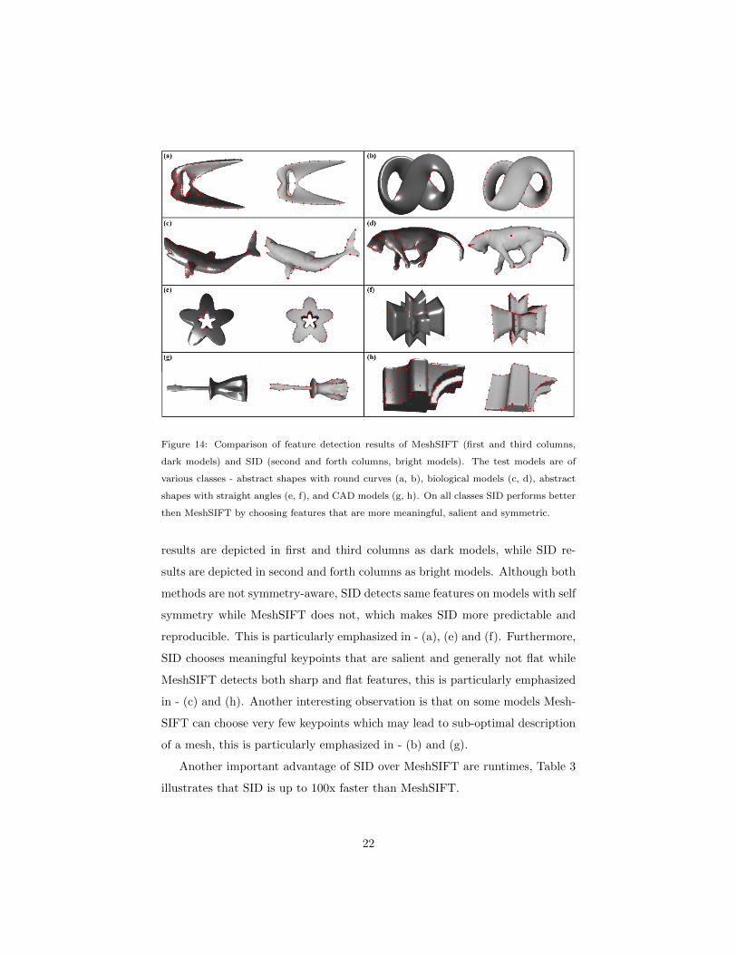
In order to further explore the differences between SID and MeshSIFT we
perform a comparison of features detected by each method on various classes of
models (see Figure 14). We used MeshSIFT [9] source code supplied by the orig-
inal authors with default parameter setting (other settings were experimented
as well, but yielded poorer results). For the comparison we use several class
of models - abstract shapes with round curves (a, b), biological models (c, d),
abstract shapes with straight angles (e, f), and CAD models (g, h). MeshSIFT
21
Page 22
Figure 14: Comparison of feature detection results of MeshSIFT (first and third columns,
dark models) and SID (second and forth columns, bright models). The test models are of
various classes - abstract shapes with round curves (a, b), biological models (c, d), abstract
shapes with straight angles (e, f), and CAD models (g, h). On all classes SID performs better
then MeshSIFT by choosing features that are more meaningful, salient and symmetric.
results are depicted in first and third columns as dark models, while SID re-
sults are depicted in second and forth columns as bright models. Although both
methods are not symmetry-aware, SID detects same features on models with self
symmetry while MeshSIFT does not, which makes SID more predictable and
reproducible. This is particularly emphasized in - (a), (e) and (f). Furthermore,
SID chooses meaningful keypoints that are salient and generally not flat while
MeshSIFT detects both sharp and flat features, this is particularly emphasized
in - (c) and (h). Another interesting observation is that on some models Mesh-
SIFT can choose very few keypoints which may lead to sub-optimal description
of a mesh, this is particularly emphasized in - (b) and (g).
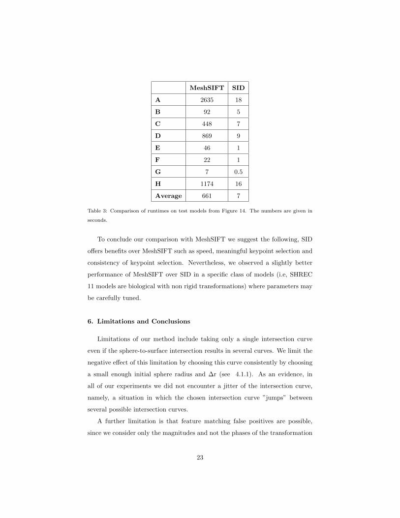
Another important advantage of SID over MeshSIFT are runtimes, Table 3
illustrates that SID is up to 100x faster than MeshSIFT.
22
Page 23
MeshSIFT SID
A 2635 18
B 92 5
C 448 7
D 869 9
E 46 1
F 22 1
G 7 0.5
H 1174 16
Average 661 7
Table 3: Comparison of runtimes on test models from Figure 14. The numbers are given in
seconds.
To conclude our comparison with MeshSIFT we suggest the following, SID
offers benefits over MeshSIFT such as speed, meaningful keypoint selection and
consistency of keypoint selection. Nevertheless, we observed a slightly better
performance of MeshSIFT over SID in a specific class of models (i.e, SHREC
11 models are biological with non rigid transformations) where parameters may
be carefully tuned.
6. Limitations and Conclusions
Limitations of our method include taking only a single intersection curve
even if the sphere-to-surface intersection results in several curves. We limit the
negative effect of this limitation by choosing this curve consistently by choosing
a small enough initial sphere radius and ∆r (see 4.1.1). As an evidence, in
all of our experiments we did not encounter a jitter of the intersection curve,
namely, a situation in which the chosen intersection curve ”jumps” between
several possible intersection curves.
A further limitation is that feature matching false positives are possible,
since we consider only the magnitudes and not the phases of the transformation
23
Page 24
of the intersection curve. However, we chose to use only the magnitudes since we
aimed to minimize dimensionality of the descriptor and we observed empirically
that the magnitude carry most of the important information.
Additional limitation of our implementation is support for watertight trian-
gular meshes only.
We have presented a novel shape descriptor for efficient matching in large
3D databases and reported experimental analysis for its performance on various
datasets. Our shape descriptor is highly distinctive, as it captures the entire
(2π) relative curvature of the neighborhood of a point. It allows even a single
feature to find a correct match with good probability in a large set of features.
Our shape descriptor is compact as it represents the intersection of a sphere
with a surface as 2 1D curves. The sphere intersection operation is simple and
relies only on the point position, thus can be defined robustly everywhere on a
surface. The use of a 2D image based representation allows efficient processing
using image processing algorithms. Our experimental results show that our
descriptor manages to capture the similarity among various dataset and is robust
against various types of deformations.
The scope of future work includes exploring additional more feature detec-
tion schemes, incorporating different techniques that capture the topological
relation among the features of the model to the graph matching, enhancing our
method with smart selection of radii to achieve scale invariance, performing
soft clustering for use of bag of features approach, handling many intersection
curves for each sphere, extending the presented descriptor to handle non wa-
tertight and point cloud datasets and evaluating the descriptor with respect to
new applications.
Acknowledgements
This work was supported by grants from the Lynn and William Frankel
Center for Computer Sciences, Ben-Gurion University, Israel 428/11, as well as
a grant from the Israeli Science Foundation. The authors would also like to
24
Page 25
thank the anonymous reviewers for the helpful suggestions and comments.
References
[1] R. C. Veltkamp, M. Hagedoorn, State of the art in shape matching (2001)
87–119.
URL http://dl.acm.org/citation.cfm?id=370792.370810
[2] E. Boyer, A. M. Bronstein, M. M. Bronstein, B. Bustos, T. Darom, R. Ho-
raud, I. Hotz, Y. Keller, J. Keustermans, A. Kovnatsky, R. Litman, J. Rein-
inghaus, I. Sipiran, D. Smeets, P. Suetens, D. Vandermeulen, A. Zaharescu,
V. Zobel, Shrec 2011: robust feature detection and description benchmark
(2011) 71–78doi:10.2312/3DOR/3DOR11/071-078.
URL http://dx.doi.org/10.2312/3DOR/3DOR11/071-078
[3] S. Belongie, J. Malik, J. Puzicha, Matching shapes 1 (2001) 454–461.
[4] C. S. Chua, R. Jarvis, Point signatures: A new representation for 3d object
recognition, Int. J. Comput. Vision 25 (1997) 63–85.
[5] A. E. Johnson, M. Hebert, Using spin images for efficient object recognition
in cluttered 3d scenes, IEEE Trans. Pattern Anal. Mach. Intell. 21 (1999)
433–449.
[6] I. Kokkinos, M. M. Bronstein, R. Litman, A. M. Bronstein, Intrinsic shape
context descriptors for deformable shapes (2012) 159–166.
[7] D. Marr, Vision: A computational investigation into the human represen-
tation and processing of visual information (1982) –.
[8] S. Biasotti, X. Bai, B. Bustos, A. Cerri, D. Giorgi, L. Li, M. Mortara,
I. Sipiran, S. Zhang, M. Spagnuolo, Shrec’12 track: stability on abstract
shapes (2012) 101–107.
[9] D. Smeets, J. Keustermans, D. Vandermeulen, P. Suetens, meshsift: Local
surface features for 3d face recognition under expression variations and
25
Page 26
partial data, Comput. Vis. Image Underst. 117 (2) (2013) 158–169. doi:
10.1016/j.cviu.2012.10.002.
URL http://dx.doi.org/10.1016/j.cviu.2012.10.002
[10] M. Flickner, H. Sawhney, W. Niblack, J. Ashley, Q. Huang, B. Dom,
M. Gorkani, J. Hafner, D. Lee, D. Petkovic, D. Steele, P. Yanker, Query
by image and video content: The qbic system, IEEE Computer 28 (1995)
23–32.
[11] C. E. Jacobs, A. Finkelstein, D. H. Salesin, Fast multiresolution image
querying (1995) 277–286.
[12] V. E. Ogle, M. Stonebraker, Chabot: Retrieval from a relational database
of images, IEEE Computer 28 (1995) 40–48.
[13] V. CASTELLI, L. BERGMAN, Image databases: Search and retrieval of
digital imagery.
[14] K. Arbter, W. E. Snyder, H. Burhardt, G. Hirzinger, Application of affine-
invariant fourier descriptors to recognition of 3-d objects, IEEE Trans.
Pattern Anal. Mach. Intell. 12 (1990) 640–647. doi:http://dx.doi.org/
10.1109/34.56206.
URL http://dx.doi.org/10.1109/34.56206
[15] E. M. Arkin, L. P. Chew, D. P. Huttenlocher, K. Kedem, J. S. B. Mitchell,
An efficiently computable metric for comparing polygonal shapes (1990)
129–137.
URL http://dl.acm.org/citation.cfm?id=320176.320190
[16] R. L. Kashyap, R. Chellappa, Stochastic models for closed boundary analy-
sis: Representation and reconstruction, IEEE Transactions on Information
Theory 27 (5) (1981) 627–637.
[17] B. K. P. Horn, Extended gaussian images, Proceedings of the IEEE 72 (12)
(1984) 1671–1686.
26
Page 27
[18] H. Delingette, M. Hebert, K. Ikeuchi, A spherical representation for the
recognition of curved objects, Computer Vision, 1993. Proceedings., Fourth
International Conference on (1993) 103–112.
[19] F. Stein, G. Medioni, Structural indexing: Efficient 3-D object recognition,
IEEE Trans. Pattern Anal. Mach. Intell. 14 (2) (1992) 125–145. doi:
10.1109/34.121785.
URL http://dx.doi.org/10.1109/34.121785
[20] C.-S. Chua, R. Jarvis, 3d free-form surface registration and object recog-
nition, International Journal of Computer Vision 17 (1) (1996) 77–99.
[21] D. Zhang, M. Hebert, Harmonic maps and their applications in surface
matching 2.
[22] M. Ankerst, G. Kastenmuller, H. P. Kriegel, T. Seidl, 3D shape histograms
for similarity search and classification in spatial databases, Advances in
Spatial Databases, 6th International Symposium, SSD’99 1651 (1999) 207–
228.
URL http://citeseerx.ist.psu.edu/viewdoc/summary?doi=10.1.1.
38.9487
[23] R. Osada, T. Funkhouser, B. Chazelle, D. Dobkin, Matching 3d models
with shape distributions (2001) 154–.
URL http://dl.acm.org/citation.cfm?id=882486.884103
[24] R. Ohbuchi, M. Nakazawa, T. Takei, Retrieving 3d shapes based
on their appearance (2003) 39–45doi:http://doi.acm.org/10.1145/
973264.973272.
URL http://doi.acm.org/10.1145/973264.973272
[25] T. Funkhouser, P. Min, M. Kazhdan, J. Chen, A. Halderman, D. Dobkin,
D. Jacobs, A search engine for 3d models, ACM Trans. Graph. 22 (2003)
83–105. doi:http://doi.acm.org/10.1145/588272.588279.
URL http://doi.acm.org/10.1145/588272.588279
27
Page 28
[26] M. Kazhdan, T. Funkhouser, S. Rusinkiewicz, Rotation invariant spherical
harmonic representation of 3d shape descriptors (2003) 156–164.
URL http://dl.acm.org/citation.cfm?id=882370.882392
[27] D. Giorgi, M. Mortara, M. Spagnuolo, 3d shape retrieval based on best
view selection (2010) 9–14doi:10.1145/1877808.1877812.
URL http://doi.acm.org/10.1145/1877808.1877812
[28] D. G. Lowe, Distinctive image features from scale-invariant keypoints,
Int. J. Comput. Vision 60 (2) (2004) 91–110. doi:10.1023/B:VISI.
0000029664.99615.94.
URL http://dx.doi.org/10.1023/B:VISI.0000029664.99615.94
[29] X. Li, I. Guskov, Multi-scale features for approximate alignment of point-
based surfaces.
URL http://dl.acm.org/citation.cfm?id=1281920.1281955
[30] A. Zaharescu, E. Boyer, K. Varanasi, R. Horaud, Surface Feature Detection
and Description with Applications to Mesh Matching.
[31] J. Sun, M. Ovsjanikov, L. Guibas, A concise and provably informative
multi-scale signature based on heat diffusion (2009) 1383–1392.
URL http://dl.acm.org/citation.cfm?id=1735603.1735621
[32] M. M. Bronstein, I. Kokkinos, Scale-invariant heat kernel signatures for
non-rigid shape recognition (2010) 1704–1711.
[33] H. Pottmann, J. Wallner, Q.-X. Huang, Y.-L. Yang, Integral invariants for
robust geometry processing, Comput. Aided Geom. Des. 26 (1) (2009) 37–
60. doi:10.1016/j.cagd.2008.01.002.
URL http://dx.doi.org/10.1016/j.cagd.2008.01.002
[34] I. Sipiran, B. Bustos, Harris 3d: a robust extension of the harris operator
for interest point detection on 3d meshes, The Visual Computer 27 (11)
(2011) 963–976.
28
Page 29
[35] T. Darom, Y. Keller, Scale-invariant features for 3-d mesh models, Image
Processing, IEEE Transactions on 21 (5) (2012) 2758–2769.
[36] F. Tombari, S. Salti, L. Di Stefano, Performance evaluation of 3d keypoint
detectors, International Journal of Computer Vision 102 (1-3) (2013) 198–
220.
[37] A. Mian, M. Bennamoun, R. Owens, On the repeatability and quality of
keypoints for local feature-based 3d object retrieval from cluttered scenes,
International Journal of Computer Vision 89 (2-3) (2010) 348–361.
[38] U. Castellani, M. Cristani, S. Fantoni, V. Murino, Sparse points matching
by combining 3d mesh saliency with statistical descriptors 27 (2008) 643–
652.
[39] M. Mortara, G. Patane, M. Spagnuolo, B. Falcidieno, J. Rossignac, Blowing
bubbles for multi-scale analysis and decomposition of triangle meshes 38
(2004) 227–248.
[40] T. Hassner, R. Basri, Single view depth estimation from examples, arXiv
preprint arXiv:1304.3915.
[41] M. B. S. S. S. Bischoff, L. Kobbelt, C. und Multimedia, Openmesh–a
generic and efficient polygon mesh data structure.
[42] G. Bradski, The opencv library, Dr. Dobb’s Journal of Software Tools.
[43] B. Dezso, A. Juttner, P. Kovacs, Lemon–an open source c++ graph tem-
plate library, Electronic Notes in Theoretical Computer Science 264 (5)
(2011) 23–45.
[44] P. Shilane, P. Min, M. Kazhdan, T. Funkhouser, The princeton shape
benchmark (2004) 167–178.
[45] C. Maes, T. Fabry, J. Keustermans, D. Smeets, P. Suetens, D. Vander-
meulen, Feature detection on 3d face surfaces for pose normalisation and
recognition (2010) 1–6.
29