Abstract The homotopy continuation methods are capable to locate multiple solutions ofnonlinear systems of equations. In this paper is presented the path-following technique usedto trace the homotopy trajectory. The spherical method is employed resizing the radius ofthe sphere at each iteration, the above based on the behavior of the radius of curvature. Alsothe Newton homotopy is applied in conjunction with the proposed methodology for tracinghomotopy curve. To prove the usefulness of the proposedmethod is applied to three exampleswith different numbers of equations obtaining successful results.
The task of located DC operating points of integrated electrical circuits is one of the mostimportant task in electrical circuit simulation. Such analysis includes finding the solutionsfor a nonlinear algebraic equation system (NAEs). The complexity of the NAEs, dependson the density of transistor fabricated on a wafer of silice and the mathematical model usedto represent the behavior of the transistor. The above causes the presence of multiple pointsof operation where the method used most often is the Newton–Raphson (NR) which is notcapable to locatemultiple points of operation. Themain reason for the use of NRmethod is itsquadratic convergence however the starting point must be close to the solution. Alternative
methods to NR are the homotopy methods, such methods are used to locate multiple DCsolutions and perhaps all the solutions if the path has more than one solution [1–3]. Continu-ation methods or homotopymethods have shown promise in solving computational problemsassociated with the simulation of circuits containing transistors. To employ the homotopymethods we embed a continuation parameter λ into a set non-linear equation system. Whenthe continuation parameter λ is set to zero then the system is reduced to equations that canbe solved easily. Homotopy equations are continuously deformed until reaching the solutionof the original system of equations. For example for finding the solution of a set of nonlinearequations F(x) = 0, where F : Rn → Rn is smooth using the continuation method. In gen-eral, this method involves incorporating the continuation parameter into a set of nonlinearequations H(x, λ),where H : Rn+1 → Rn [4–7]. The computational efficiency of homotopymethods depends on the homotopy formulation as well as the curve-tracing algorithm andthe initial point [4,5,7–11]. The usefulness of homotopy methods depends on the type ofa circuits descriptive equations. Such methods are becoming a viable alternative in circuitsimulation, where they can be used to resolve convergence difficulties and to find multipleoperation points. These methods are slower than conventional methods but their speed canoften be improved by careful implementation [12–17].
In this paper is organizable in the following sections, first the introduction is submit-ted, we briefly explain the characteristics of the Newton homotopy used in this proposedwork is present in “Newton Homotopy” section, later to trace the curve of homotopy is usedthe spherical method explained in “The Spherical Algorithm” section, proposed methodol-ogy to change the radius of the spheres in the spherical method is presented in “ProposedMethodology to Accelerate the Course of the Curve on the Spherical Algorithm” section,numerical examples are solved using the proposed methodology in “Numerical Examples”section, finally the discussion of results and conclusions are shown in “Discussion” and“Conclusions” sections, respectively.
Newton Homotopy
The operating point problem for a DC network is formulated as a system of non-linearequations to be solved F(x) = 0. The Newton homotopy has similar properties to the NRmethod, meaning that every homotopy path in the regular domain crosses at the same solutionpoint. TheNewton homotopy [11,18] is described by the following set of nonlinear equations:
H(x, λ) = F(x) − (1 − λ)
[g(x0)
0
]= 0. (1)
In circuit simulation applications, x ∈ Rn is the vector of node voltages, F(x) gives the setof Kirchhoff’s Current Law equations at each node, where λ ∈ R is called the continuationparameter and g(x0) is F(x) assessed at the initial point.
The solutions in DC are founded at λ = 1 on the solution curve, changing the start pointg(x0) we can trace the another solution curves. If the starting point is selected properly thenit possible find all solutions of the system [18].
The Spherical Algorithm
Tracing solution curves is a problem encountered in homotopy methods, where is requiredsuitable path-tracking techniques. The curve tracing algorithm can be divided in two types;
123
Int. J. Appl. Comput. Math (2016) 2:421–433 423
Fig. 1 Path tracking usingspheres
the first is based on the predictor–corrector algorithmwhereas the second are piecewise-linearalgorithms [19]. These algorithm are sophisticated and very efficient, notwithstanding thesecurve algorithm tracing algorithms are not widely used in practical applications; difficultiesprimarily linked to the implementation of these algorithms are the theory and programming.The spherical algorithm (SA) based predictor–corrector algorithm is used for geometricallyclear interpretation besides its easy implementation in programming [20–23]. The SA algo-rithm consists of trace the curve using spheres of dimension n+1,where n+1 is the numberof variables of the equation system to be solved and continuation parameter. For tracing solu-tion curves a starting point is chosen as the same point used wherein, the center of the firstsphere; then spheres are traced following the shape of the curve using predictor–correctoralgorithm as shown in Fig. 1.
Equation (2) that describe the sphere with center at C and radius r is expressed by:
S(X) = (x1 − c1)2 + (x2 − c2)
2 + · · · + (xn+1 − cn+1)2 − r2 = 0. (2)
The equation of the sphere is update at every iteration using the new center at C(c1, c2, . . . ,cn+1). The homotopy is applied to equilibrium equations F(x) to obtain a equation systemincreased as (3) with n + 1 equations and n + 1 variables.
H1 (F1(x), λ) = 0,H2 (F2(x), λ) = 0,...
Hn (Fn(x), λ) = 0,S (x1, x2, . . . , xn, λ) = 0.
(3)
To follow the tracing solutions, the spheres are plotted using the predictor–corrector algo-rithm, where the predictor is calculated as a sum of vectors and the predictor point is used tofind the correction point by solving the system of equations as (3).
Predictor–Corrector
– The predictor point is given using the Fig. 1, where the center of the first sphere o1 andthe center of the consecutive sphere o2 are used to obtain the step predictor.
123
424 Int. J. Appl. Comput. Math (2016) 2:421–433
Fig. 2 Sphere intersecting withthe curve at two points
Fig. 3 Reversion strategyproposed
– The corrector point uses NR method, setting as a starting point the predictor point andsolving (3), where can be localized at least two solutions: one lies in the forward directiono4 and the other in the backward direction o2 (see Fig. 2). The forward solution can beconsidered as a success of the algorithm, nonetheless if the backward solution is obtained,the algorithm fails; such case of failure is known as “reversion” phenomenon of the SA.To solve reversion problem is applied the calculus the angles of their normal vector to asphere for the solutions o2 and o4, instead of comparing o2 and o4 directly, we use theangles of their normal vectors for an efficient comparison. After detecting the reversionphenomenon, we have to modify the corrector step by increasing the radius a δr (whereδr is an increase of the radius) inducing the corrector step to converge to the forwardsolution [23,24] (Fig. 3).
– Find zero strategy the finding zero strategy should start after the trajectory crosses solutionline λ = 1 [25,26]. A functional way consist by monitoring the change of sign of �λ
after the corrector step. This procedure is realized by multiplying �λ of two consecutivepredictor steps.
sign(�λ j+1�λ j
) �= −1. (4)
– Interpolate solutions when the trajectory crosses the line solution the point (k1, k2) aretaken to implement multidimensional interpolation to approximate the solution. Interpo-lation is performed using the command “ArrayInterpolation” language Maple [24].
123
Int. J. Appl. Comput. Math (2016) 2:421–433 425
C
P
Fig. 4 Spherical algorithm
Proposed Methodology to Accelerate the Course of the Curveon the Spherical Algorithm
Homotopy methods are characterized by slowness to the path tracking. We want to solve thesystem of equations H(x · λ) = 0, using Newton homotopy and for tracking the solutioncurve use the SA. Size radius for spheres is fixed for the SA was reported in [21]. Thereforemaking the radius of each sphere varies according to the form of the solution curve (seeFig. 4).
As the first step of the proposed methodology is to calculate the radius of curvature by
ρ =∣∣∣∣∣(1 + (x ′
i )2)
32
x ′′i
∣∣∣∣∣ , (5)
where x ′i , x
′′i are numerical derivatives of first and second order, respectively evaluated for
current iteration. Numerical approximation for the first derivative is used in calculating theradius of curvature by
x ′i = xi − xi−1
h, (6)
where xi and xi−1 are current iteration and preceding iteration, respectively, h is the Euclideandistance between them. The second-order derivative also used to calculate the radius ofcurvature can be analogously calculated as:
x ′′i = x ′
i − x ′i−1
h, (7)
where x ′i is the first derivative evaluated in the current iteration and x
′i−1 is first order derivative
evaluated in the previous iteration (see Fig. 5).Using (7) and (6) can be calculated (5) for each variable x1, x2, . . . , xn corresponds to
the number of system variables. Then is used arithmetic mean for the radius of curvature isgiven by
ρav = ρx1 + ρx2 + · · · + ρxn
n. (8)
123
426 Int. J. Appl. Comput. Math (2016) 2:421–433
Fig. 5 Proposed variable radius
ix
1−ix h
jx
1−jx
Fig. 6 Hyperbolic tangentfunction
The radius of the sphere expressed as the variable r is calculated using the hyperbolic tangentfunction (9)
r = f (ρav) = tanh (ρav) = eρav − e−ρav
eρav + e−ρav. (9)
The function there are also a pair of horizontal asymptotes is know as a sigmoid functionand is a bounded differentiable real function that is defined for all real input values and has apositive derivative at each point. Figure6 shows the function behavior, using as parametersthe radius of curvature.
Equation (8) is a hyperbolic tangent function used to find the value of the radius of thesphere. To accelerate change radio size can increase the hyperbolic function exponent usinga constant K by
r = f (ρav) = eKρav − 1
eKρav + 1, (10)
where K is an integer that allows the function to have is an abrupt change in the range ofallowed values. At each iteration the curvature radius is calculated to obtain the radius of thesphere suitable to trace homotopy curve during the course of the bend solution.
Numerical Examples
For exemplify the effectiveness of the methodology of fixed radius versus variable radius,three study case are submitted.
123
Int. J. Appl. Comput. Math (2016) 2:421–433 427
Case Study with Two Variables
The first study case is a circuit with a two diodes, one voltage source (E) an a resistor (R) asshown in Fig. 7. In where the range of the radius of the hypersphere is taking of 0.009–0.1,knowing that most of the time the radius size will have the most value.
The mathematical expression that represents the non-linear model having the form of apolynomial:
The formulation used in this work is the Newton homotopy (12), then spherical method withfixed radius is applied, for this first example the radio fixed size is r = 0.03. For the sameexample, we change the variable radius methodology proposed in this work, for which arange of possible values for the radius of the sphere where the minimum value is the fixedvalue of radius 0.3 and the maximum value is 0.1 to avoid jumps between solution path. Wecan see Fig. 8, the result of comparison between fixed radius and the methodology of variableradius.
Fig. 7 Two tunnel diode circuit
(a) (b)
Fig. 8 a Radius size constant. b Radius size variable
123
428 Int. J. Appl. Comput. Math (2016) 2:421–433
Table 1 Numerical results for the first case study
CPU time (s) Iteration numbers
Same size radio (0.03) 7.03 205
Different size radio (0.03–0.1) 6.1 146
Table 2 All solutions found forthe first case study
Initial point (0, 0.3) Solutions (v1, v2)
S1 (2.3052, 0.7055)
S2 (1.6663, 0.7393)
S3 (0.2282, 0.8286)
S4 (0.2198, 1.6729)
S5 (1.7026, 1.8090)
S6 (2.2775, 1.8574)
S7 (2.2247, 3.6930)
S8 (1.7755, 3.7071)
S9 (0.1997, 3.7542)
12V
0.1K 0.1K
8K 8K
4K 4K
30K
1K
0.1K
10K
4K 10K
1K
i 1
2
3
4 5
6
7
8
9
10
1112
13
Fig. 9 Example circuit with 14 variables
Comparing the same curve solution but in the Fig. 8a using fixed radius display a curveas solid lines while for Fig. 8b points are drawn wide apart because the radius of the sphereis changed with respect to changes in the curve form solution. Table1 shows the results asthe computation time and the total number of iterations. The result shows advantages in theuse of fixed radius regarding sphere of variable radius. For this case study all solutions weresuccessfully found as shown in Table2.
Case Study with 14 Variables
The following circuit is described by a system of nonlinear equations with 14 variablesIE , v1, v2, v3, v4, v5, v6, v7, v8, v9, v10, v11, v12, v13. This circuit contain four transis-tor and one diode as shown in Fig. 9.
123
Int. J. Appl. Comput. Math (2016) 2:421–433 429
The equilibrium equations are obtained from the modified nodal analysis by:
f1 = 37
20, 000v1 − 1
4000v2 − 1
4000v6 − 1
1000v9 − 1
4000v12 − 1
10, 000v13 + IE ,
f2 = − 1
40, 000v1 + 3
8000v2 + 3
8000v5 + 9.90E − 09 exp40v4−40v3
+1E − 10 − 1E − 08 exp40v4−40v2 ,
f3 = 1
100v3 − 1E − 08 exp40v4−40v3 +9.90E − 09 + 1E − 10 exp40v4−40v2 ,
f4 = 1
8000v4 − 1
8000v6 + 1E − 10 exp40v4−40v3 −1E − 08 + 9.90E
−09 exp40v4−40v2 ,
f5 = 1
8000v2 + 1
8000v5 + 1E − 10 exp40v5−40v7 −1E − 08
+9.90E − 09 exp40v5−40v6 ,
f6 = 1
4000v1 − 1
8000v4 + 3
8000v6 + 9.90E − 09 exp40v5−40v7
+1.010E − 08 exp40v5−40v6 −1E − 08 exp40v8−40v6 ,
f7 = 1
100v7 − 1E − 08 exp40v5−40v7 +9.90E − 09 + 1E − 10 exp40v5−40v6 ,
f8 = 1
30, 000v8 − 1
30, 000v9 + 1E − 08 exp40v8−40v6 −1.E − 08,
f9 = 1
1000v1 − 1
30, 000v8 + 31
30, 000v9 + 9.90E − 09 exp40v11−40v10 +1E − 10
+1E − 08 exp40v11−40v9 ,
f10 = 1
100v10 − 1E − 08 exp40v11−40v10 +9.90E − 09
+1E − 10 exp40v11−40v9 ,
f11 = 1
10, 000v11 − 1
10, 000v12 + 1e − 10 exp40v11−40v10 −1E − 08
+9.9E − 09 exp40v11−40v9 ,
f12 = − 1
4000v1 − 1
10, 000v11 + 7
20, 000v12 + 9.9E − 12 exp40v13 +1E − 10
−1E − 08 exp40v13−40v12 ,
f13 = − 1
10, 000+ 11
10, 000v13 + 1E − 10 exp40v13 −1E − 08
+9.90E − 09 exp40v13−40v12 ,
f14 = v1 − 12.
The exponential function in the Ebers–Moll is used. Then Newton homotopy is applied toembedding the continuation parameter λ into a set of nonlinear equations H(x, λ) and thencurve is traced using proposed methodology, we obtain the solution in Tables3 and 4.
While the CPU time also is reduced for fixed radius and variable radius respectively. Theprojection of variable versus the λ parameter can be graphed, Fig. 10 shows IE and v13.
Fig. 10 a Radius size constant. b Radius size variable
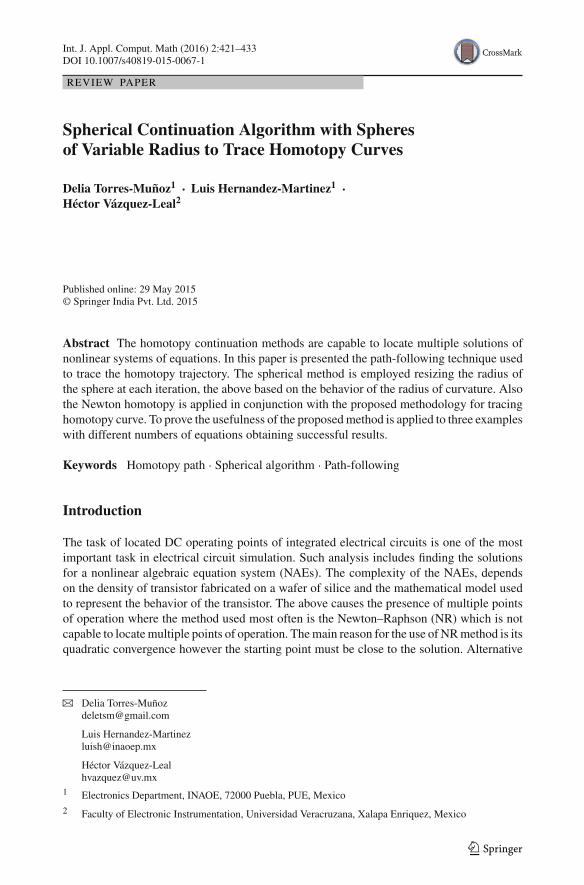
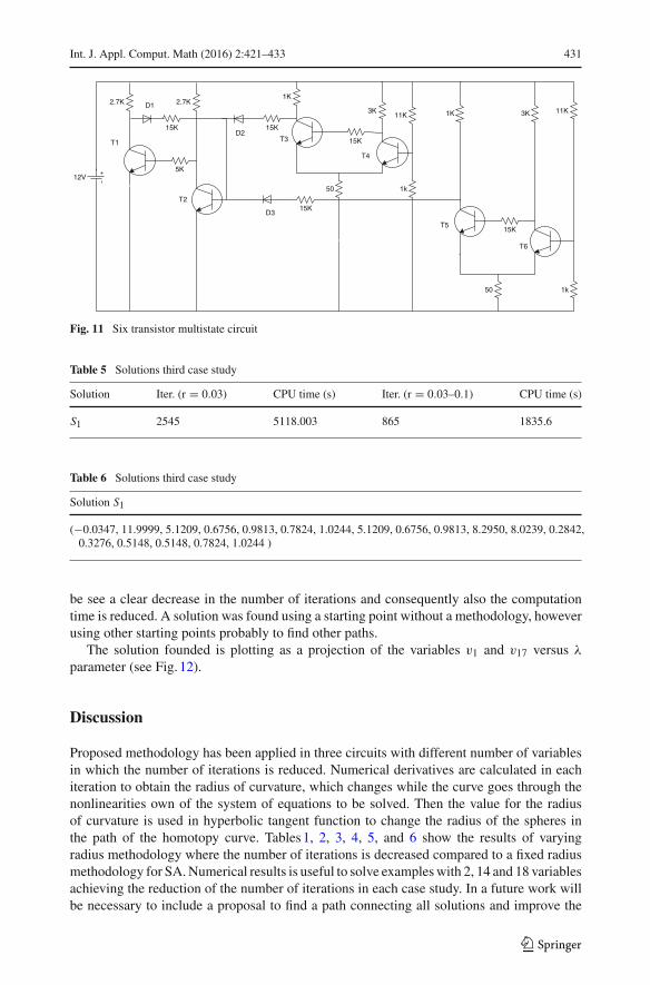
Case Study with 18 Variables
Consider the following case study containing 6 transistors, 3 diodes and 18 resistors;the Fig. 11 shows the circuit. In this example, we applied the proposed algorithm tothe same Newton homotopy function as above example, we choose a starting point as(−15, −15, −15, −15, −15, −15, −15,−15, −15, −15, −15, −15, −15, −15, −15,−15, −15, −15). Tables5 and 6 shows results of tracing the homotopy path, where can
123
Int. J. Appl. Comput. Math (2016) 2:421–433 431
15K
2.7K 2.7K
5K
15K
1K
15K
50
3K11K
1k
15K
50 1k
15K
1K 3K 11K
12V
D1
D2
D3
T1
T2
T3
T4
T5
T6
Fig. 11 Six transistor multistate circuit
Table 5 Solutions third case study
Solution Iter. (r = 0.03) CPU time (s) Iter. (r = 0.03–0.1) CPU time (s)
be see a clear decrease in the number of iterations and consequently also the computationtime is reduced. A solution was found using a starting point without a methodology, howeverusing other starting points probably to find other paths.
The solution founded is plotting as a projection of the variables v1 and v17 versus λ
parameter (see Fig. 12).
Discussion
Proposed methodology has been applied in three circuits with different number of variablesin which the number of iterations is reduced. Numerical derivatives are calculated in eachiteration to obtain the radius of curvature, which changes while the curve goes through thenonlinearities own of the system of equations to be solved. Then the value for the radiusof curvature is used in hyperbolic tangent function to change the radius of the spheres inthe path of the homotopy curve. Tables1, 2, 3, 4, 5, and 6 show the results of varyingradius methodology where the number of iterations is decreased compared to a fixed radiusmethodology for SA.Numerical results is useful to solve exampleswith 2, 14 and 18 variablesachieving the reduction of the number of iterations in each case study. In a future work willbe necessary to include a proposal to find a path connecting all solutions and improve the
123
432 Int. J. Appl. Comput. Math (2016) 2:421–433
(a) (b)
Fig. 12 a Radius size constant. b Radius size variable
results obtained. Nonetheless finding a curve with all connected solutions is presented as anarea of opportunity to work on the starting point of homotopy.
Conclusions
The radius of curvature provides sufficient information on the prediction of how the curvewillbehave in the next iteration. Then the SA has been adapted to the variable-radius conformingto the shape of the curve. Using three study cases describing the behavior of electrical circuits,we show the use of variable radius for spheres in the SA yields better computation times inthe simulations because the less number of iterations in each simulation. In the first casestudy all solutions are found while in the following case studies solutions depend stronglyon the starting point.
and State of the Art. Academic, London (1987)3. Melville, R.C., Trajkovic, L., Fang, S.-C., Watson, L.T.: Artificial parameter homotopy methods for the
DC operating point problem. IEEE Trans. Comput. Aided Des. Integr. Circuits Syst. 12(6), 861–877(1993)
4. Green, M.M.: An efficient continuation method for use in globally convergent DC circuit simulation.In: Proceedings of the 1995 URSI International Symposium on Signals, Systems, and Electronics, 1995.ISSSE ’95, vol. 40(8), pp. 497–500 (1995). doi:10.1109/ISSSE.1995.498040
5. Green, M.M., Melville, R.C.: Sufficient conditions for finding multiple operating points of DC circuitsusing continuation methods. In: 1995 IEEE International Symposium on Circuits and Systems, 1995.ISCAS ’95, vol. 40(8), pp. 117–120 (1995). doi:10.1109/ISCAS.1995.521465
6. Trajkovic, L., Melville, R.C., Fang, S.-C.: Finding DC operating points of transistor circuits using homo-topy methods. In: IEEE International Symposium on Circuits and Systems, 1991, vol. 2, 40(8), pp.758–761 (1991). doi:10.1109/ISCAS.1991.176473
7. Trajkovic, L., Melville, R.C., Fang, S.-C.: Improving DC convergence in a circuit simulator using ahomotopy method. In: Proceedings of the IEEE 1991 Custom Integrated Circuits Conference, 1991, vol.40(8) (1991). doi:10.1109/CICC.1991.1640328.1/1-8.1/4
16. Bates, D.J., Hauenstein, J.D., Sommese, A.J.,Wampler, C.W.: Stepsize control for adaptivemultiprecisionpath tracking. Contemp. Math. 496, 21–31 (2009)
17. Bates, D.J., Hauenstein, J.D., Sommese, A.J., Wampler II, C.W.: Adaptive multiprecision path tracking.SIAM J. 46(2), 722–746 (2000)
18. Ushida, A., Yamagami, Y., Nishio, Y., Kinouchi, I., Inoue, Y.: An efficient algorithm for finding multipleDC solutions based on the SPICE-oriented Newton homotopy method. IEEE Trans. Comput. Aided Des.Integr. Circuits Syst. 0278–0070, 337–348 (2002)
19. Yamamura, K., Ohshimar, T.: Finding all solutions of piecewise-linear resistive circuits using linearprogramming. IEEE Trans. Circuits Syst. I 45(4), 434–445 (1998)
20. Vazquez-Leal, H., Castaneda Sheissa, R., Rabago Bernal, F., Hernandez-Martinez, L., Sarmiento-Reyes,A., Filobello-Nino,A.U.: Poweringmultiparameter homotopy-based simulationwith a fast path-followingtechnique. ISRN Appl. Math. 1 (2011)
21. Yamamura, K.: Simple algorithms for tracing solution curves. IEEE Trans. Circuits Syst. I 40(8), 537–541(1993)
22. Chua, L.O., Ushida, A.: A switching-parameter algorithm for finding multiple solutions of nonlinearresistive circuits. Int. J. Circuit Theory Appl. 4, 115–239 (1976)
23. Torres-Munoz,D.,Hernandez-Martinez, L.,Vazquez-Leal,H.: Improved spherical continuation algorithmby nonlinear circuit. In: 2013 IEEE 56th International Midwest Symposium on Circuits and Systems(MWSCAS), pp. 61–64 (2003)
24. Torres-Munoz, D., Vazquez-Leal, H., Hernandez-Martinez, L., Sarmiento-Reyes, A.: Improved sphericalcontinuation algorithm with application to the double bounded homotopy (dbh). Comput. Appl. Math.33(1), 147–161 (2014)
25. Sosonkina, M., Watson, L.T., Stewart, D.E.: Note on the end game in homotopy zero curve tracking.ACM Trans. Math. Softw. 22(3), 281–287 (1996)
26. Vazquez-Leal, H., Hernandez-Martinez, L., Sarmiento-Reyes, A., Castaneda-Sheissa, R.: Numericalcontinuation scheme for tracing the double bounded homotopy for analysing nonlinear circuits. In: Pro-ceedings of the 2005 International Conference on Communications, Circuits and Systems, 2005, vol. 2(2005)


![Bifurcation Analysis of a Generic Pusher Type Transport ... · PDF filenumerical continuation algorithm. ... In this work, AUTO 2000 [8] bifurcation and continuation algorithm is used](https://static.documents.pub/doc/80x56/5aa145fc7f8b9a1f6d8b9fe3/bifurcation-analysis-of-a-generic-pusher-type-transport-continuation-algorithm.jpg)