Splined speed control using SpAM (Speed-based Acceleration Maps) for an autonomous ground vehicle David Paul Anderson Thesis submitted to the faculty of the Virginia Polytechnic Institute and State University in partial fulfillment of the requirements for the degree of Masters of Science In Mechanical Engineering Dr. Charles F. Reinholtz, Chairman Dept. of Mechanical Engineering, Embry Riddle Aeronautical University Dr. Alfred L. Wicks, Assistant Chairman Dept. of Mechanical Engineering Dr. Dennis W. Hong Dept. of Mechanical Engineering January 14, 2008 Blacksburg, VA
Transcript
Splined speed control using SpAM (Speed-based Acceleration Maps)
for an autonomous ground vehicle
David Paul Anderson
Thesis submitted to the faculty of the Virginia Polytechnic Institute and State University in partial fulfillment of the requirements for the degree of
Masters of Science
In
Mechanical Engineering
Dr. Charles F. Reinholtz, Chairman
Dept. of Mechanical Engineering, Embry Riddle Aeronautical University
Dr. Alfred L. Wicks, Assistant Chairman
Dept. of Mechanical Engineering
Dr. Dennis W. Hong
Dept. of Mechanical Engineering
January 14, 2008
Blacksburg, VA
ii
Splined speed control using SpAM (Speed-based Acceleration Maps) for
an autonomous ground vehicle
David Paul Anderson
Abstract
There are many forms of speed control for an autonomous ground vehicle currently in development. Most use a simple PID controller to achieve a speed specified by a higher-level motion planning algorithm. Simple controllers may not provide a desired acceleration profile for a ground vehicle. Also, without extensive tuning the PID controller may cause excessive speed overshoot and oscillation.
This paper examines an approach that was designed to allow a greater degree of control while reducing the computing load on the motion planning software.
The SpAM+PI (Speed-based Acceleration Map + Proportional Integral controller) algorithm outlined in this paper uses three inputs: current velocity, desired velocity and desired maximum acceleration, to determine throttle and brake commands that will allow the vehicle to achieve its correct speed. Because this algorithm resides on an external controller it does not add to the computational load of the motion planning computer. Also, with only two inputs that are needed only when there is a change in desired speed or maximum desired acceleration, network traffic between the computers can be greatly reduced.
The algorithm uses splines to smoothly plan a speed profile from the vehicle’s current speed to its desired speed. It then uses a lookup table to determine the correct pedal position (throttle or brake) using the current vehicle speed and a desired instantaneous acceleration that was determined in the splining step of the algorithm. Once the pedal position is determined a PI controller is used to minimize error in the system.
The SpAM+PI approach is a novel approach to the speed control of an autonomous vehicle. This academic experiment is tested using Odin, Team Victor Tango’s entry into the 2007 DARPA Urban Challenge which won 3rd place and a $500,000 prize. The evaluation of the algorithm exposed both strengths and weaknesses that guide the next step in the development of a speed control algorithm.
iii
Acknowledgments
I would like to thank a number of people for making my graduate studies both possible
and successful.
First I would like to thank my family for always guiding and supporting the decisions that
I make. Thank you to my girlfriend for putting up with my hours in the lab and for being there
for me, especially for the last few weeks of work.
I would like to thank every member of Team Victor Tango for their tireless work in
making Odin the success that he was. I would like to especially thank Patrick Currier, Jesse
Farmer, David VanCovern, and all of the undergraduates with which I worked to create, wire,
and install all of the hardware needed to turn a Ford hybrid Escape into an autonomous vehicle.
I would also like to thank Mike Webster for coining the “SpAM” acronym; without his lyrical
insight my work would not have been nearly as tasty.
Lastly I would like to thank my advisors for their support. Dr Charles Reinholtz was
instrumental in my decision to work towards my master’s degree as well as continually guiding
me through the process. Dr Al Wicks for always making sure that the team was on task and for
supporting us in every area possible; and Dr Dennis Hong for believing in me and helping me to
believe in myself. Thank you all.
iv
Table of Contents
Chapter 1: Introduction 1
1.1 Motivation 1
Chapter 2: Overview of Mathematical Techniques 3
2.1 PID 4
2.2 Splines 5
2.3 Speed-based Acceleration Map 6
2.4 Fuzzy Logic 8
Chapter 3: Other Approaches 9
Chapter 4: Test Platform 12
Chapter 5: Control Algorithm Description 16
5.1 Description of a PID Controller 18
5.2 Spline Decision and Generation 21
5.3 Description of SpAM 25
5.3.1 Test to obtain the response of the vehicle 26
5.3.2 Processing the data 27
5.4 Implementation of SpAM 30
Chapter 6: Conclusions 41
6.1 Future Work 42
Appendix A: Testing Results 44
v
Acronyms and Abbreviations
ACC Adaptive Cruise Control
ACC+Stop&Go Adaptive Cruise Control plus Stop and Go
CAN Controller Area Network
cRIO National Instruments CompactRIO
CVT Continuously Variable Transmission
DARPA Defense Advanced Research Projects Agency
DOF Degrees Of Freedom
FPGA Field Programmable Gate Array
HI Human Interface
Hz Hertz
I/O Input/Output
OEM Original Equipment Manufacturer
PI Proportional-Integral controller
PID Proportional-Integral-Derivative controller
PD Proportional-Derivative controller
RPM Revolutions Per Minute
SpAM Speed-based Acceleration Map
SpAM+PI Speed-based Acceleration Map plus Proportional Integral controller
SUV Sport Utility Vehicle
THS Toyota Hybrid System
V Voltage
vi
List of Figures
Figure 1-1 Schematic of a centrifugal governor. 2 Figure 2-1. Example Brake Speed-based Acceleration Map (SpAM). 6 Figure 2-2. Fuzzy Height Example Membership Values. 8 Figure 4-1 Schematic of Ford Hybrid Escape Driveline. 13 Figure 5-1 Block diagram of a PID controller. 19 Figure 5-2 Example Speed-based Acceleration Map (SpAM). 25 Figure 5-3 Raw velocity vs time data from all brake runs. 27 Figure 5-4 Throttle Speed-based Acceleration Map. 28 Figure 5-5 Braking Speed-based Acceleration Map. 29 Figure 5-6 SpAM algorithm flow. 30 Figure 5-7 Vehicle response for SpAM and PI Controller running 32 at 1.5 m/s2 Amd. Figure 5-8 Vehicle Response for PI Controller at 1.5 m/s2 Amd. 33 Figure 5-9 Modified SpAM algorithm flow. 35 Figure 5-10 Vehicle Response for SpAM+PI Algorithm with 36 1.5 m/s2 Amd. Figure 5-11 Vehicle Response for SpAM+PI Algorithm with 37 0.75 m/s2 Amd. Figure 5-12 Vehicle Response for SpAM+PI Algorithm with 38 2.25 m/s2 Amd. Figure 5-13 Vehicle Response for 1.5 m/s2 Amd during a Hill Climb. 39 Figure 5-14 Vehicle Response for 1.5 m/s2 Amd during a Hill Descent. 40
vii
Figure A-1 Vehicle Response for PI Controller with 0.75 m/s2 Amd. 44 Figure A-2 Vehicle Response for PI Controller with 2.25 m/s2 Amd. 44 Figure A-3 Response for SpAM and PI Running Continuously 45 at 0.75 m/s2 Amd. Figure A-4 Vehicle Response for SpAM and PI running continuously 45 with 2.25 m/s2 Amd.
viii
List of Tables
Table 4-1 National Instruments Compact RIO (cRIO) Modules used 14 to convert a Ford Hybrid Escape to DBW. Table 5-1 Effects of increasing PID parameters: Kp, Ki and Kd 19 Table A-1 Vehicle Response Statistics for SpAM and PI controller 46 Running Continuously Table A-2 Vehicle Response Statistics for SpAM+PI controller 46 Table A-3 Vehicle Response Statistics for PI controller 46
1
Chapter 1
Introduction
1.1 Motivation
A vehicle being able to maintain its speed autonomously is nothing new. The first
vehicular speed control was demonstrated in the 1910s by the Peerless Motor Company of
Cleveland, Ohio. Their system consisted of a centrifugal governor [2].
The centrifugal, or flyball, governor was first used for engine control by James Watt in
1788 to control the speed of his steam engine. This governor which had been previously used to
control the speed of waterwheels and windmills was one of the first examples of linking the
output of a mechanism to its input; this idea of feedback embodies the basic idea of automation
[3].
Watt’s governor can be seen in figure 1-1. It is described by Robert Thurston at the
Stevens Institute of Technology.
Two heavy iron or brass balls, BB', were suspended from pins, CC', in a little cross-piece carried on the head of a vertical spindle, AA', driven by the engine. The speed of the engine varying, that of the spindle changed correspondingly, and the faster the balls were swung the farther they separated. When the engine's speed decreased, the period of revolution of the balls was increased, and they fell back toward the spindle. Whenever the velocity of the engine was uniform, the balls preserved their distance from the spindle and remained at the same height, their altitude being determined by the relation existing between the force of gravity and centrifugal force in the temporary position of equilibrium…
The arms carrying the balls, or the balls themselves, are pinned to rods, MM’, which are connected to a piece, NN', sliding loosely on the spindle. A score, 7, cut
2
in this piece engages a lever, V, and, as the balls rise and fall, a rod, W, is moved, closing and opening the throttle-valve, and thus adjusting the supply of steam in such a way as to preserve a nearly fixed speed of engine [10].
Figure 1-1. Schematic of a centrifugal governor. The centrifugal, or flyball, governor regulates the speed of a primary force mover using centrifugal force on the weights which are attached to a lever to change the input to the mover. This picture courtesy of the Robert Thurston of the Stevens Institute of Technology.
The 1958 Chrysler Imperial was the first production vehicle to use the Teeter cruise
control approach, the foundation of today’s system. Teeter’s approach measured driveshaft
rotations to estimate the ground speed of the vehicle and used a solenoid to vary throttle position
as needed [2]. Cruise control today is still based on error between the set point and actual
vehicle speed but the control is done using software control theory as opposed to mechanical
methods.
Modern cruise control works well for a driver that does not want to be burdened with the
application of the throttle; however, the control system falls short of the needs for speed control
of an autonomous vehicle. These shortcomings include: the allowable error is too great for
precise control, the system will not apply the brake simply to achieve desired speed, the systems
are not capable of reverse, desired acceleration is not configurable, and most commercially
available systems will not engage at less than 25 miles per hour.
3
Chapter 2
Overview of Mathematical Techniques
The techniques used in the development of the SpAM algorithm include the commonly
used PID controller, splining, and a less commonly used speed-based acceleration map. Each of
these techniques will be quickly reviewed in this section before they are more thoroughly
explored later in the paper.
In this paper the terms “velocity” and “speed” will be used interchangeably. While the
meanings are not identical this usage is accurate because the velocity of a vehicle can only be in
one direction, the direction of travel. Since this algorithm deals only with speed of the vehicle
and not the steering it can be assumed that a local coordinate system is placed on the vehicle and
always points in the direction of travel. This way, both “velocity” and “speed” will have
identical meanings.
4
2.1 PID
A proportional-integral-derivative (PID) controller is a mathematical controller that
allows management of a process variable using the desired and actual values of the process, for
instance, the velocity of a vehicle. The process variable, velocity, can be maintained given a
desired speed which is the set point, and the actual velocity of the vehicle.
As the name suggests a PID controller consists of three terms, a proportional, an integral
and a derivative term. Each of these terms contains a gain, usually denoted K, which determines
the amount of influence that each term will exert over the response of the system. Before a PID
controller can be effective for determining control of a system, the controller needs to be tuned.
To tune a controller means to adjust the values of each of the gains: Kp, Ki, Kd, so that the
response of the system is desirable. Unfortunately, tuning a PID is not solely a science but also
an art. As in all systems it is not possible to obtain the “perfect” response of a system; ie, instant
rise time, zero overshoot, instant settle time, and zero error; but a balance must be achieved so
that the system behaves favorably. The math and tuning of a PID controller will be more
thoroughly explored in a later section.
5
2.2 Splines
Splining is a technique that stitches mathematical curves together in a smooth and
continuous fashion. A spline can be any number of curves, or curves of any order or type. For
example, a spline could consist of a simple line of the form
xaay 211 += , (2-1)
followed by:
)sin(2 xby = , (2-2)
finished by:
54
2
3
3
2
4
13 cxcxcxcxcy ++++= . (2-3)
The requirement is that the functions must form a differentiable curve, meaning that the values
and the slopes at the interfaces must be equal.
In a polynomial spline the number of degrees of freedom, DOF, of the spline is
determined by the order of the curves used. Each variable allows for another DOF. This means
that if one needs to have control of nine parameters then there needs to be a total of nine
variables within the spline’s equations. Again, this technique will be explained more thoroughly
in a later section.
6
2.3 Speed-based Acceleration Map
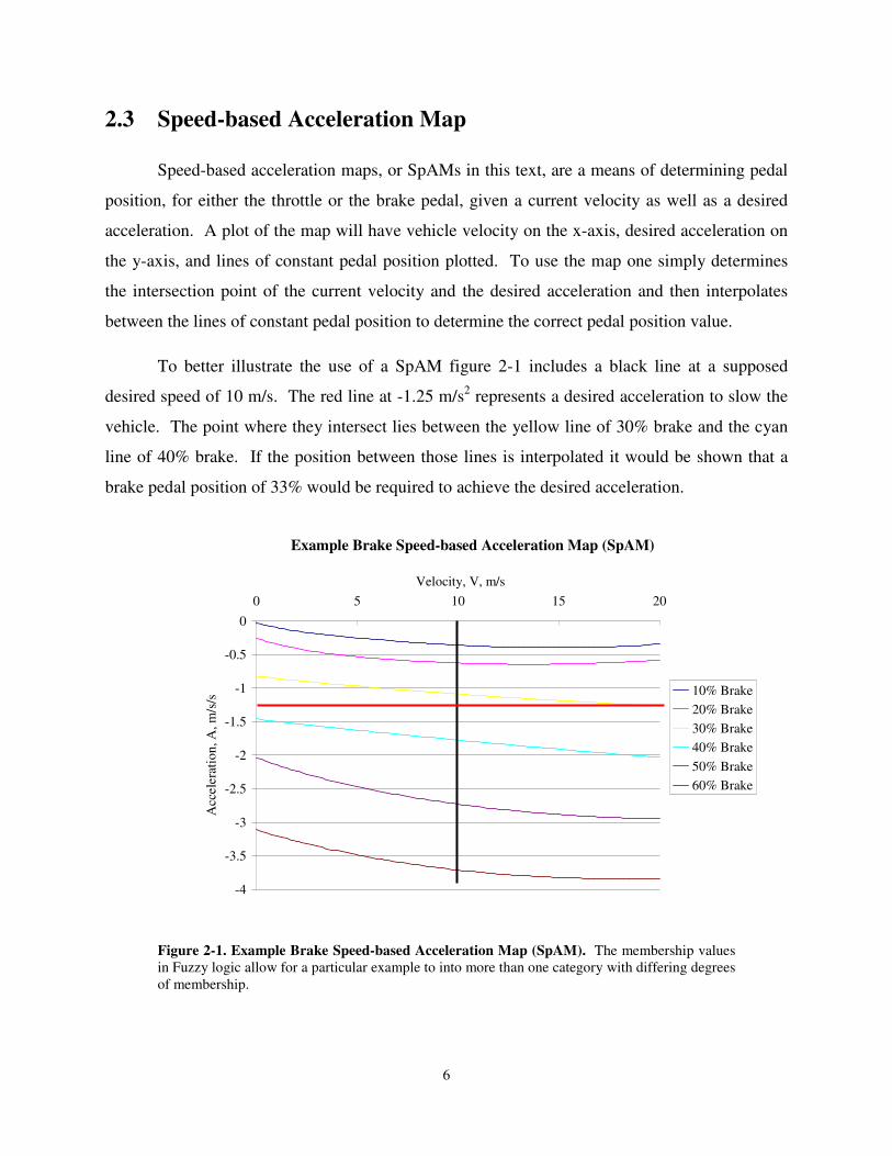
Speed-based acceleration maps, or SpAMs in this text, are a means of determining pedal
position, for either the throttle or the brake pedal, given a current velocity as well as a desired
acceleration. A plot of the map will have vehicle velocity on the x-axis, desired acceleration on
the y-axis, and lines of constant pedal position plotted. To use the map one simply determines
the intersection point of the current velocity and the desired acceleration and then interpolates
between the lines of constant pedal position to determine the correct pedal position value.
To better illustrate the use of a SpAM figure 2-1 includes a black line at a supposed
desired speed of 10 m/s. The red line at -1.25 m/s2 represents a desired acceleration to slow the
vehicle. The point where they intersect lies between the yellow line of 30% brake and the cyan
line of 40% brake. If the position between those lines is interpolated it would be shown that a
brake pedal position of 33% would be required to achieve the desired acceleration.
Example Brake Speed-based Acceleration Map (SpAM)
-4
-3.5
-3
-2.5
-2
-1.5
-1
-0.5
0
0 5 10 15 20
Velocity, V, m/s
Acc
eler
atio
n, A
, m
/s/s
10% Brake
20% Brake
30% Brake
40% Brake
50% Brake
60% Brake
Figure 2-1. Example Brake Speed-based Acceleration Map (SpAM). The membership values in Fuzzy logic allow for a particular example to into more than one category with differing degrees of membership.
7
A single SpAM does not cover all of the situations needed when controlling the velocity
of a vehicle. For this reason, two maps were used for this algorithm, one describing the throttle
characteristics of the vehicle, and one describing the braking characteristics.
Although this was not the technique employed, it is possible however, to use three maps.
One for throttle acceleration, one for throttle deceleration, and one for brake deceleration. This
technique would be more accurate because a given throttle-pedal position could have two
acceleration values associated with it. One value would be a positive acceleration for the case
when the vehicle is traveling at a low speed, and have a negative acceleration for the case of a
higher vehicle velocity. This higher velocity would require more power than is available from
the drive train at such a throttle position. This level of accuracy was determined to not be
necessary because of the use of a PID controller to minimize error.
8
2.4 Fuzzy Logic
Fuzzy logic can be described as the practical side to Fuzzy Set Theory. Fuzzy logic is
best used for systems that contain qualitative information instead of quantitative information. It
is used for systems that may not have definite values to distinguish the cases that are handled.
For instance, suppose that a computer program is written to categorize a list of people as “short”,
“average”, and “tall”. A classical “predicate logic” program could be written where everyone
that is less than 5’10” is “short”, everyone taller than 6’2” is “tall”, and then all others are
“average”. But who is to say that 5’10” is the cut off? When driving a road if the posted speed
limit is 30 mph than there is a definite cutoff between speeding and not speeding, but in the
height example this is not the case.
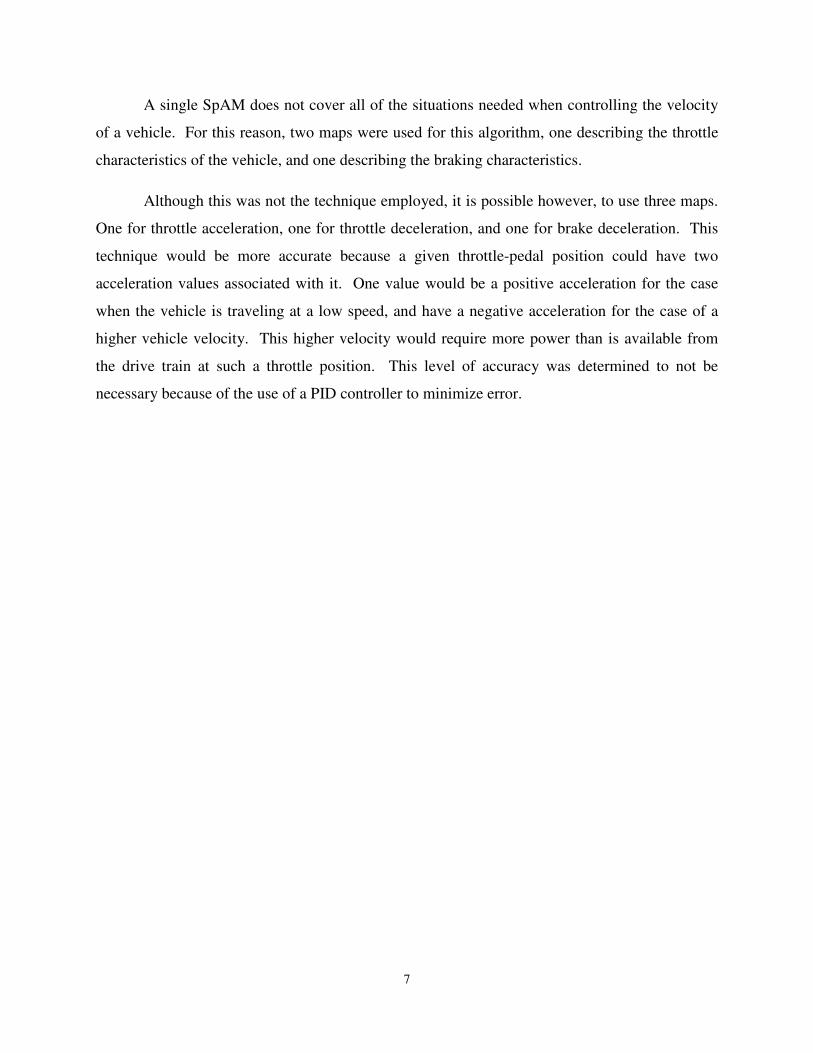
In fuzzy logic, membership values are created that describe the degree of truth for a given
situation. This degree of truth is a value from 0 to 1. It is possible that a particular case will fall
into more than one category, such as a man that is 5’8” could be considered both “short” and
“average”. This is illustrated in figure 2-2 in the areas where “short” and “average” or “average”
and “tall” overlap.
Fuzzy Height Example Membership Values
0
1
Height
Deg
ree o
f M
em
ber
ship
Figure 2-2. Fuzzy Height Example Membership Values. The membership values in Fuzzy logic allow for a particular example to into more than one category with differing degrees of membership.
Short Average Tall
S&A A&T
48 52 56 60 64 68 72 76 80
Height, inches
Fuzzy Height Example Membership Values
Deg
ree
of
Mem
ber
ship
9
Chapter 3
Other Approaches
Low level autonomous speed control is not a topic that is discussed in great deal in many
papers concerning the operation of autonomous vehicles. The majority of approaches discuss the
higher level decision making software, the software that decides the desired speed of the vehicle,
but will not mention details as to how the desired speed was achieved. The papers simply state
that a PID controller was used to attain the proper velocity. The topics in these publishings do
not perfectly parallel the approach described within this paper. The SpAM+PI approach
described in this paper attempts to allow the higher level motion planning software to divorce
itself from the problem of “how does the vehicle get from its current speed to its desired speed?”
This approach allows the motion planning software to simply output a desired speed as well as
how quickly that speed needs to be achieved.
The papers that do discuss the implementation of speed control are usually focused on
adaptive cruise control (ACC) with the extension of stop and go maneuvers. One such paper is
titled “ACC+Stop&Go Maneuvers With Throttle and Brake Fuzzy Control” [7]. The fuzzy logic
approach described in this paper with regards to the throttle pedal includes four input variables,
one output variable, and five rules. Because this approach deals with the decision making behind
ACC, the rules that are used to maintain following distance are included in this set of rules. Only
the rules and theory relevant to the SpAM approach will be discussed. The definitions for the
variables used in the rules are:
1) Speed Error: This is the difference between the current speed and the user-preset speed, which is expressed as
10
dpresetSpeeedCurrentSpeSpeedError −= .
It is the error signal whose value has to be as low as possible. Therefore, the rules are generally designed to reduce its value, for instance, by releasing the pedal if the speed is too high. Its fuzzy variable representation is named “speed_error.”
2) Acceleration: This is the derivative of the speed at instant t. It is associated to a fuzzy variable named “acceleration.” The acceleration is calculated as
t
edCurrentSpeedCurrentSpeonAccelerati tt
∆
−=
−1
That may provide oscillating values; they have to be filtered to get a smoother value. For this purpose, a digital Fourier filter has been implemented with a sampling rate of 10 Hz, a filtering cutting rate of 1 Hz, and 4 coefficients [7].
To use these variables, the controller determines the degree of truth of “SpeedError is greater
than zero”, this degree of truth will control the appropriate amount of additional throttle; if the
degree of truth of “SpeedError is less than zero” is itself not zero, and there is not sufficient gap
between cars it will apply less throttle. If acceleration is greater than zero the control will apply
more throttle, and if acceleration is less than zero and there is not enough space between
vehicles the vehicle will throttle down. It needs to be remembered that the preceding rules do
not depend on the values of acceleration and SpeedError but the degree of truth associated with
those variables.
Upon initial inspection of these rules they seem to mimic a proportional-integral-
derivative controller, and the author confirms this observation:
There is a parallelism between the fuzzy controller and a classic PD: We could
say that the rules involving the “speed_error” behave like a proportional
controller component and the rules involving the “acceleration” behave like a
derivative component. This means that the “speed_error” rules adjust the throttle
pressure when the speed of the car is not at the target value, and the
“acceleration” rules smooth out the actuation of this command, just like the
damping effect of a D-control term [7].
The results of the fuzzy logic approach are good but not exceptional. From the published
data there seems to be a lag in the actual speed from the desired speed of approximately four
seconds in most responses.
11
Another reason to use a more traditional, quantitative approach, can be devised because
of what Joseph Putney describes of fuzzy logic in his paper, “Reactive Navigation of an
Autonomous Ground Vehicle Using Dynamic Expanding Zones”. Here he mentions that “Fuzzy
logic excels when there is a lack of quantitative information and only qualitative knowledge
exists. Fuzzy logic is not a good solution for high precision, high accuracy control.” (p30) This
is not the case in speed control where a current speed and a desired speed can be quantified.
Another reason that fuzzy logic was not an attractive option was because the amount of
data that is needed to make it useful. Daniel Abramovitch of the Hewlett-Packard Laboratories
gave a talk in which he states that “Most fuzzy logic controllers are compared to PID controllers”
[1]. But that is only after he states “Many fuzzy logic success stories use more sensors than the
controller that they improve on” [1]. Why implement a control strategy that is comparable to the
current control but requires more input, which adds hardware complexity and cost as well
additional development effort?
12
Chapter 4
Test Platform
The vehicle used to develop this algorithm was a 2005 Ford Hybrid Escape. This
particular vehicle was Team Victor Tango’s entry “Odin” into the 2007 DARPA Urban
Challenge.
The use of the hybrid electric Ford Escape provides numerous advantages in the areas of on-board power generation, reliability, safety and autonomous operation. As required by DARPA, the drive-by-wire conversion does not bypass any of the stock safety systems. Since the stock steering, shifting and throttle systems on the Hybrid Escape are already drive-by-wire, these systems can be controlled electronically by emulating the command signals, eliminating the complexity and failure potential associated with the addition of external actuators” [9].
As Charles Reinholtz mentioned the throttle, steering shifting is all drive-by-wire, this means
that in order to achieve brake-by-wire the team added an actuator. This actuator was added
because tapping into the brake control signal would have compromised the integrity of an
essential safety system of the vehicle.
The Hybrid Escape uses a CAN, controller area network, bus for the majority of its
communications. This bus contained data that would be useful to the team. It was simply a
matter of reading from this bus and acquiring information already known to the vehicle, such as
vehicle speed.
Another benefit to using the Hybrid Escape was the lack of a traditional transmission,
either manual or automatic. The Hybrid Escape uses two electric motors and a traditional
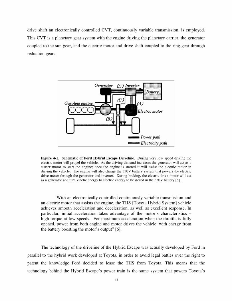
gasoline engine to provide its propulsive force, figure 4-1. To couple the engine, motors, and
13
drive shaft an electronically controlled CVT, continuously variable transmission, is employed.
This CVT is a planetary gear system with the engine driving the planetary carrier, the generator
coupled to the sun gear, and the electric motor and drive shaft coupled to the ring gear through
reduction gears.
Figure 4-1. Schematic of Ford Hybrid Escape Driveline. During very low speed driving the electric motor will propel the vehicle. As the driving demand increases the generator will act as a starter motor to start the engine; once the engine is started it will assist the electric motor in driving the vehicle. The engine will also charge the 330V battery system that powers the electric drive motor through the generator and inverter. During braking, the electric drive motor will act as a generator and turn kinetic energy to electric energy to be stored in the 330V battery [6].
“With an electronically controlled continuously variable transmission and an electric motor that assists the engine, the THS [Toyota Hybrid System] vehicle achieves smooth acceleration and deceleration, as well as excellent response. In particular, initial acceleration takes advantage of the motor’s characteristics – high torque at low speeds. For maximum acceleration when the throttle is fully opened, power from both engine and motor drives the vehicle, with energy from the battery boosting the motor’s output” [6].
The technology of the driveline of the Hybrid Escape was actually developed by Ford in
parallel to the hybrid work developed at Toyota, in order to avoid legal battles over the right to
patent the knowledge Ford decided to lease the THS from Toyota. This means that the
technology behind the Hybrid Escape’s power train is the same system that powers Toyota’s
14
hybrid vehicles. The engine is the primary means of locomotion. However, at low speeds, while
driving down hill, or while moving in reverse the electric drive motor will solely create the
movement. When the driving load increases the generator will act as a starter motor and start the
gasoline engine. Once started the engine’s power will be split through the planetary system,
some of the power will be sent to the wheels to aid the drive motor and some will be sent to the
generator so that the battery pack will be recharged through the use of an inverter. During
braking, the electric drive motor will act as a generator and will convert kinetic energy to electric
energy to be stored in the battery pack. To aid in braking, the system also uses a conventional
four-wheel disc brake system.
Because the throttle, shifter, and power steering were already by-wire, the team would
only need to reproduce the signals needed to generate the desired control. The computer used to
do this was determined to be the National Instruments CompactRIO system. The CompactRIO
is a real-time processor coupled to an FPGA backplane. The backplane contains eight
independent input/output ports for which National Instruments offers a variety of I/O modules.
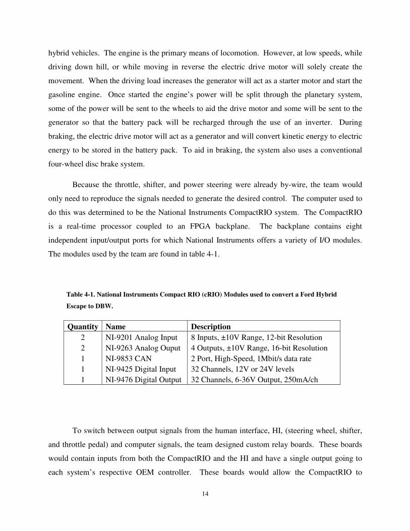
The modules used by the team are found in table 4-1.
Table 4-1. National Instruments Compact RIO (cRIO) Modules used to convert a Ford Hybrid
Escape to DBW.
Quantity Name Description
2 NI-9201 Analog Input 8 Inputs, ±10V Range, 12-bit Resolution
2 NI-9263 Analog Ouput 4 Outputs, ±10V Range, 16-bit Resolution
1 NI-9853 CAN 2 Port, High-Speed, 1Mbit/s data rate
1 NI-9425 Digital Input 32 Channels, 12V or 24V levels
1 NI-9476 Digital Output 32 Channels, 6-36V Output, 250mA/ch
To switch between output signals from the human interface, HI, (steering wheel, shifter,
and throttle pedal) and computer signals, the team designed custom relay boards. These boards
would contain inputs from both the CompactRIO and the HI and have a single output going to
each system’s respective OEM controller. These boards would allow the CompactRIO to
15
monitor the output of the HI and have control over a set of relays on each board. These relays
would allow the CompactRIO to replace the HI output with its own. By monitoring the HI
output the team was able to engineer additional safety into the system. For instance, in order for
the CompactRIO to command autonomous control of the vehicle the shifter needs to be in the
“neutral” position. If at any time the vehicle displays unsafe operation, a safety driver simply
needs to place the shifter in “drive” and he will have full control of the vehicle.
Another concern for safety lead to the manner in which brake-by-wire was achieved.
Because there was sufficient room underneath the dashboard, a linear actuator was employed to
push on the brake pedal. The actuator does not affect the safety driver’s ability to apply the
brake because the point of interaction of the actuator is high on the pedal’s lever arm. Also, the
actuator only pushes on the lever arm, it is not rigidly coupled to it; meaning that the driver has
the ability to add to the computer’s braking decision.
16
Chapter 5
Control Algorithm Description
Many velocity control algorithms depend on the sole use of a PID controller. Assuming
that the computer making the higher-level decisions is not going to “micromanage” the velocity
control of the vehicle, a simple PID controller will tend to “over use” the throttle and brake
pedals. This “over use” occurs because the PID must be tuned to react quickly so that in
situations of quick response the desired velocity is met immediately. However, this inevitably
leads to situations where an immediate response by either the throttle or the brake will lead to
undesirable vehicle motion; such as a situation of slight desired negative acceleration. In this
situation the aggressively tuned PID will apply the brake, even though simply letting off of the
throttle may have produced the desired result.
A fuzzy logic controller can be used to control the velocity as well. However, concerns
have been expressed that because fuzzy logic is not a set mathematical expression speed control
may not be the correct application. “Fuzzy logic is derived from fuzzy set theory dealing with
reasoning that is approximate rather than precisely deduced from classical predicate logic. It can
be thought of as the application side of fuzzy set theory dealing with well thought out real world
expert values for a complex problem” [4].
For these reasons the algorithm developed has the ability to more elegantly control the
speed of a vehicle than a simple PID controller and be more precise than fuzzy logic. The
elegance of this algorithm comes from two places. First, it will predict an acceleration curve that
the vehicle should follow so that driving is done in a comfortable and efficient manner, without
17
harsh changes in acceleration. And second, it uses a SpAM specifically developed for the
intended vehicle. Using this map the algorithm makes a “guess” at the correct values for the
brake and accelerator before control error is minimized using a PID controller. This “guess” or
feed forward part of the control loop allows the controller to be tuned to optimize characteristics
such as rise time, overshoot, oscillation, and settle time.
18
5.1 Description of a PID Controller
The simplest approach to speed control is a proportional controller. With a proportional
controller the amount of throttle that should be applied in order to accelerate the vehicle to some
desired set point is determined using a single term. In this controller the error between the
desired speed and the actual speed, is multiplied by some constant, Kp, and the result determines
the amount of throttle to be applied.
A proportional controller is very simple in practice but it does not produce desired
characteristics. The main downfall of the controller is that either it will take a long time to reach
the set point or it will overshoot. The reason for the overshoot is that the response of this
controller is not influenced by the rate at which the error is growing (or shrinking), or by the
length of time which the error has occurred. This overshoot does not just occur on the initial
rise, but will continue to occur both in the positive and negative direction causing oscillation
about the set point.
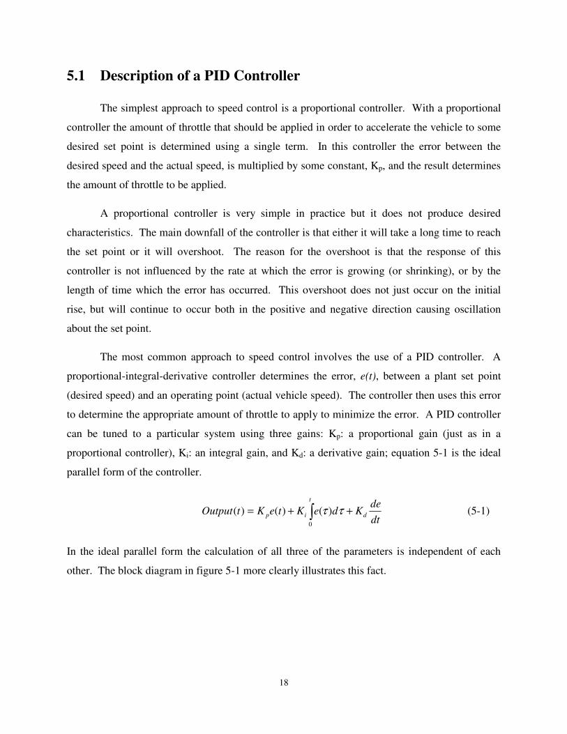
The most common approach to speed control involves the use of a PID controller. A
proportional-integral-derivative controller determines the error, e(t), between a plant set point
(desired speed) and an operating point (actual vehicle speed). The controller then uses this error
to determine the appropriate amount of throttle to apply to minimize the error. A PID controller
can be tuned to a particular system using three gains: Kp: a proportional gain (just as in a
proportional controller), Ki: an integral gain, and Kd: a derivative gain; equation 5-1 is the ideal
parallel form of the controller.
dt
deKdeKteKtOutput d
t
ip ++= ∫0
)()()( ττ (5-1)
In the ideal parallel form the calculation of all three of the parameters is independent of each
other. The block diagram in figure 5-1 more clearly illustrates this fact.
19
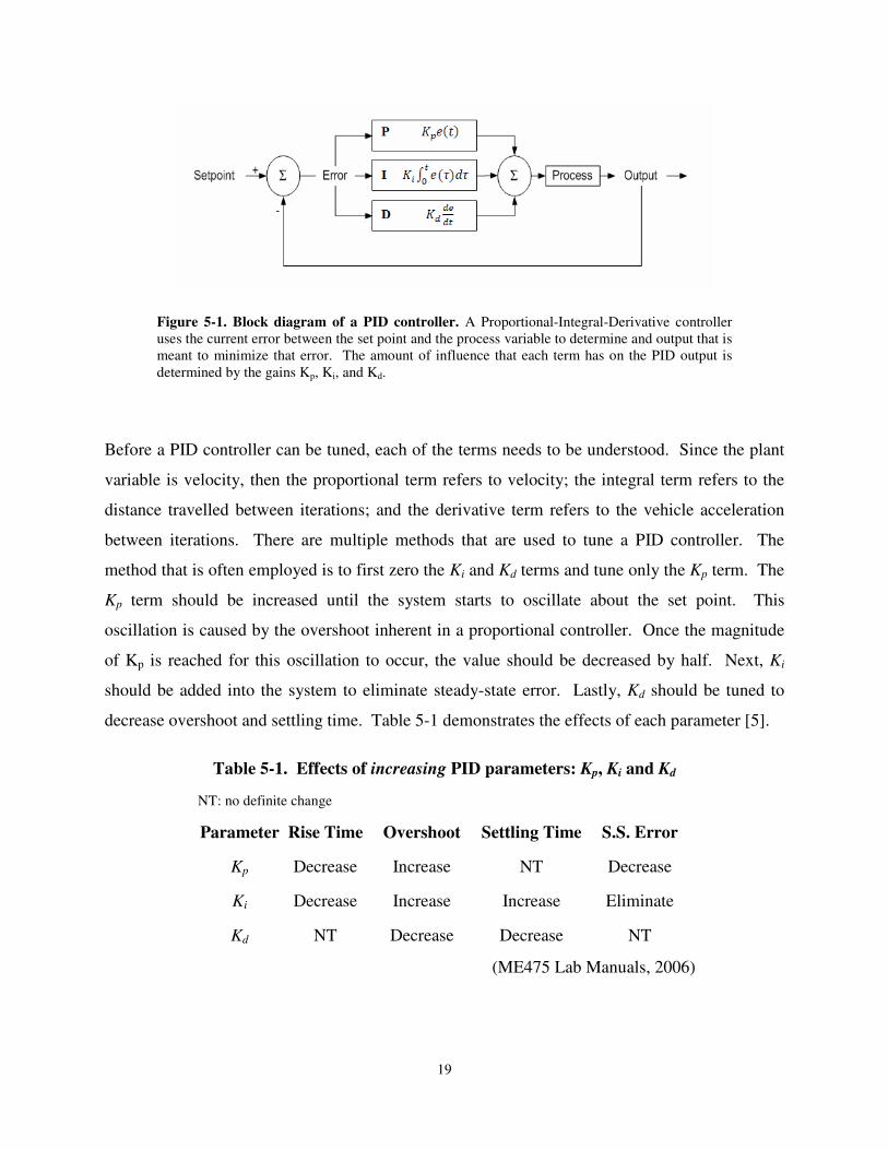
Figure 5-1. Block diagram of a PID controller. A Proportional-Integral-Derivative controller uses the current error between the set point and the process variable to determine and output that is meant to minimize that error. The amount of influence that each term has on the PID output is determined by the gains Kp, Ki, and Kd.
Before a PID controller can be tuned, each of the terms needs to be understood. Since the plant
variable is velocity, then the proportional term refers to velocity; the integral term refers to the
distance travelled between iterations; and the derivative term refers to the vehicle acceleration
between iterations. There are multiple methods that are used to tune a PID controller. The
method that is often employed is to first zero the Ki and Kd terms and tune only the Kp term. The
Kp term should be increased until the system starts to oscillate about the set point. This
oscillation is caused by the overshoot inherent in a proportional controller. Once the magnitude
of Kp is reached for this oscillation to occur, the value should be decreased by half. Next, Ki
should be added into the system to eliminate steady-state error. Lastly, Kd should be tuned to
decrease overshoot and settling time. Table 5-1 demonstrates the effects of each parameter [5].
Table 5-1. Effects of increasing PID parameters: Kp, Ki and Kd
NT: no definite change
Parameter Rise Time Overshoot Settling Time S.S. Error
Kp Decrease Increase NT Decrease
Ki Decrease Increase Increase Eliminate
Kd NT Decrease Decrease NT
(ME475 Lab Manuals, 2006)
20
Many times the designer intends to use a PID controller; however, during the implementation
any value for Kd causes the system to go unsteady. The derivative term is especially sensitive to
noise within the system. To eliminate noise one can implement some form of filtering.
Unfortunately, the derivative term is also sensitive to the lag that is inevitable with any form of
effective filter. For this reason the Kd term will often be left as zero and the designer will settle
on using a PI controller.
It is very possible that a suitable set of gains will not be sufficient over the entire
operating region of the system. This could be due to many factors. In the case of a vehicle,
inconsistency could be caused by the transmission shifting to a new gear or because of the power
available from the engine at different RPM. To handle these situations gain scheduling can be
implemented. Gain scheduling involves using different values for Kp, Ki and/or Kd depending on
the value of some input, such as current operating point or current gear.
21
5.2 Spline Decision and Generation
In order to achieve a smooth ride within the vehicle, certain aspects of the driven velocity
profile had to be true. These aspects include: any curve defining the vehicle speed had to be
continuous and differentiable, any change in desired velocity must be gradual and therefore not
cause a discontinuity within the velocity curve, and the curve should define a path to the desired
velocity without overshoot or oscillation.
It was apparent that the desired velocity profile would resemble either an “S ”, or one
that was upside down. This was determined because the majority of the time the vehicle would
be moving from a state of zero acceleration and some speed to another state of zero acceleration
at a different speed. Upon initial inspection it was determined that a single low order
polynomial, exponential, or trigonometric function would not adequately describe this desired
profile. Any one of the preceding functions will not give the “S ” profile as well as provide the
degree of control desired. For this reason splining was employed. Splining is a method of
stitching together individual functions that each operate within distinct portions of the operating
range, as described in equation 5-2.
1
1
2
1
),(
),()(
xx
xx
xq
xqxq
≥
<
= (5-2)
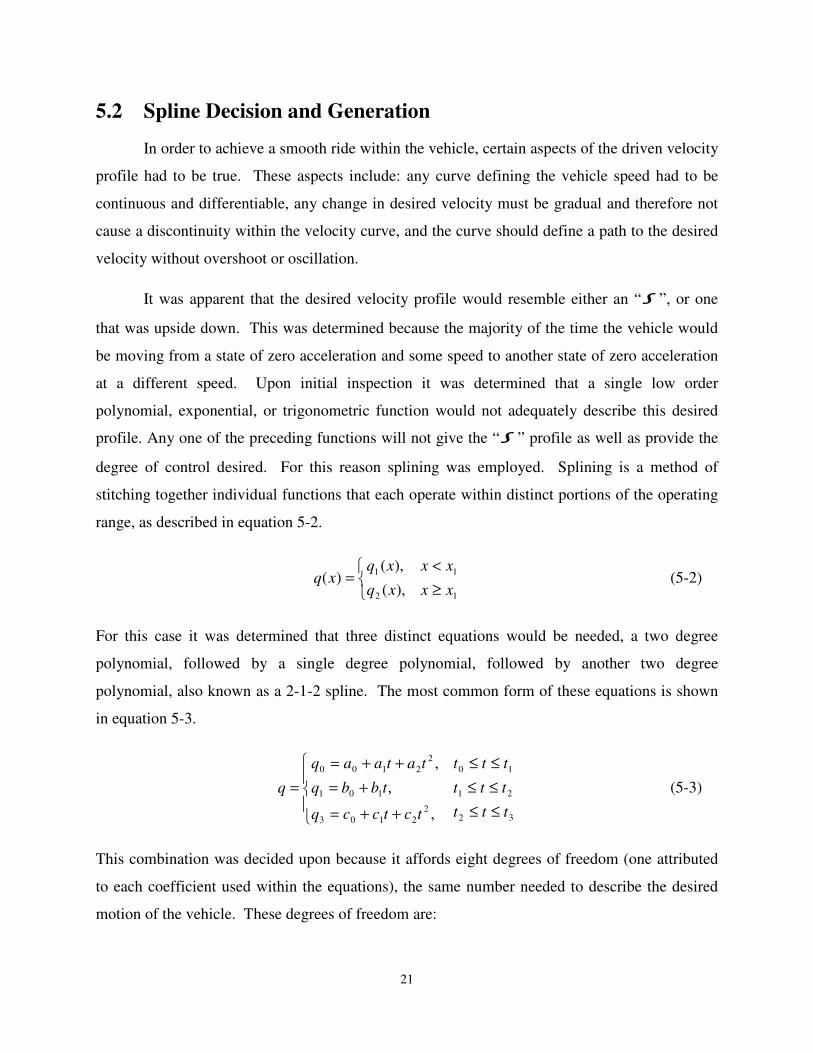
For this case it was determined that three distinct equations would be needed, a two degree
polynomial, followed by a single degree polynomial, followed by another two degree
polynomial, also known as a 2-1-2 spline. The most common form of these equations is shown
in equation 5-3.
32
21
10
2
2103
101
2
2100
,
,
,
ttt
ttt
ttt
tctccq
tbbq
tataaq
q
≤≤
≤≤
≤≤
++=
+=
++=
= (5-3)
This combination was decided upon because it affords eight degrees of freedom (one attributed
to each coefficient used within the equations), the same number needed to describe the desired
motion of the vehicle. These degrees of freedom are:
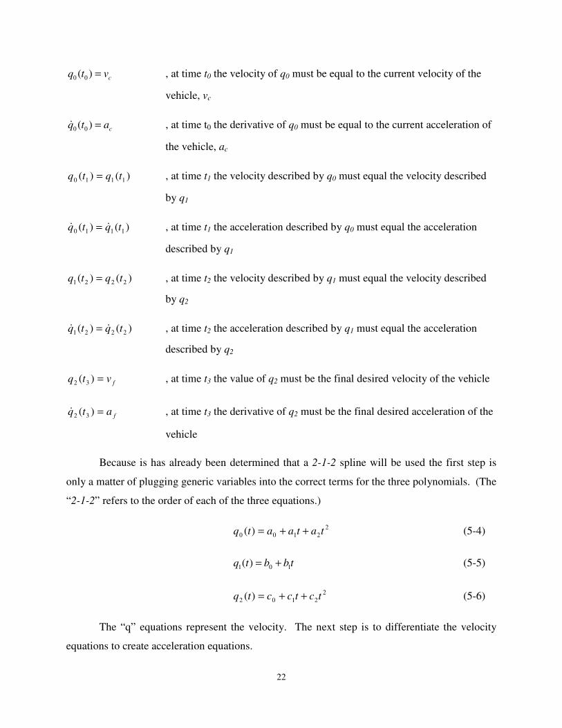
22
cvtq =)( 00 , at time t0 the velocity of q0 must be equal to the current velocity of the
vehicle, vc
catq =)( 00& , at time t0 the derivative of q0 must be equal to the current acceleration of
the vehicle, ac
)()( 1110 tqtq = , at time t1 the velocity described by q0 must equal the velocity described
by q1
)()( 1110 tqtq && = , at time t1 the acceleration described by q0 must equal the acceleration
described by q1
)()( 2221 tqtq = , at time t2 the velocity described by q1 must equal the velocity described
by q2
)()( 2221 tqtq && = , at time t2 the acceleration described by q1 must equal the acceleration
described by q2
fvtq =)( 32 , at time t3 the value of q2 must be the final desired velocity of the vehicle
fatq =)( 32& , at time t3 the derivative of q2 must be the final desired acceleration of the
vehicle
Because is has already been determined that a 2-1-2 spline will be used the first step is
only a matter of plugging generic variables into the correct terms for the three polynomials. (The
“2-1-2” refers to the order of each of the three equations.)
2
2100 )( tataatq ++= (5-4)
tbbtq 101 )( += (5-5)
2
2102 )( tctcctq ++= (5-6)
The “q” equations represent the velocity. The next step is to differentiate the velocity
equations to create acceleration equations.
23
taatq 210 2)( +=& (5-7)
11 )( btq =& (5-8)
tcctq 212 2)( +=& (5-9)
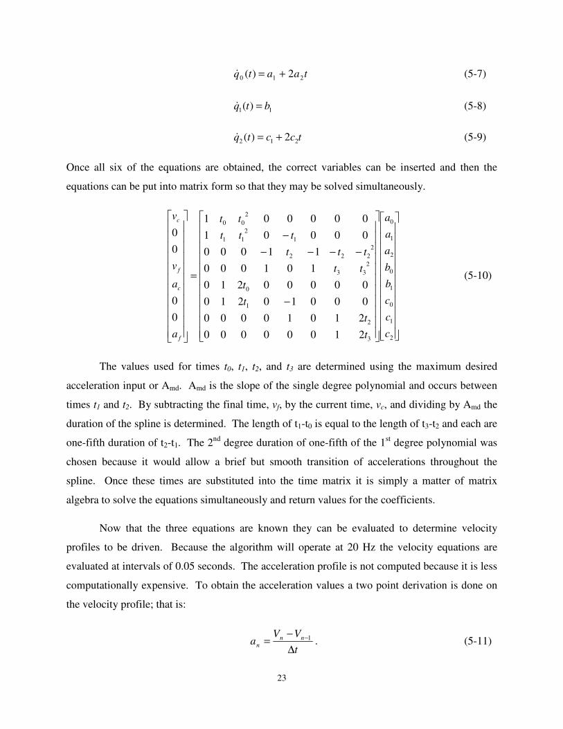
Once all six of the equations are obtained, the correct variables can be inserted and then the
equations can be put into matrix form so that they may be solved simultaneously.
−
−−−−
−
=
2
1
0
1
0
2
1
0
3
2
1
0
2
33
2
222
1
2
11
2
00
21000000
21010000
00010210
00000210
101000
11000
00001
000001
0
0
0
0
c
c
c
b
b
a
a
a
t
t
t
t
tt
ttt
ttt
tt
a
a
v
v
f
c
f
c
(5-10)
The values used for times t0, t1, t2, and t3 are determined using the maximum desired
acceleration input or Amd. Amd is the slope of the single degree polynomial and occurs between
times t1 and t2. By subtracting the final time, vf, by the current time, vc, and dividing by Amd the
duration of the spline is determined. The length of t1-t0 is equal to the length of t3-t2 and each are
one-fifth duration of t2-t1. The 2nd degree duration of one-fifth of the 1st degree polynomial was
chosen because it would allow a brief but smooth transition of accelerations throughout the
spline. Once these times are substituted into the time matrix it is simply a matter of matrix
algebra to solve the equations simultaneously and return values for the coefficients.
Now that the three equations are known they can be evaluated to determine velocity
profiles to be driven. Because the algorithm will operate at 20 Hz the velocity equations are
evaluated at intervals of 0.05 seconds. The acceleration profile is not computed because it is less
computationally expensive. To obtain the acceleration values a two point derivation is done on
the velocity profile; that is:
t
VVa nn
n∆
−=
−1 . (5-11)
24
Once the discrete values of the profiles are determined they are stored in queues and sent
sequentially to the next step, the SpAM algorithm.
25
5.3 Description of SpAM
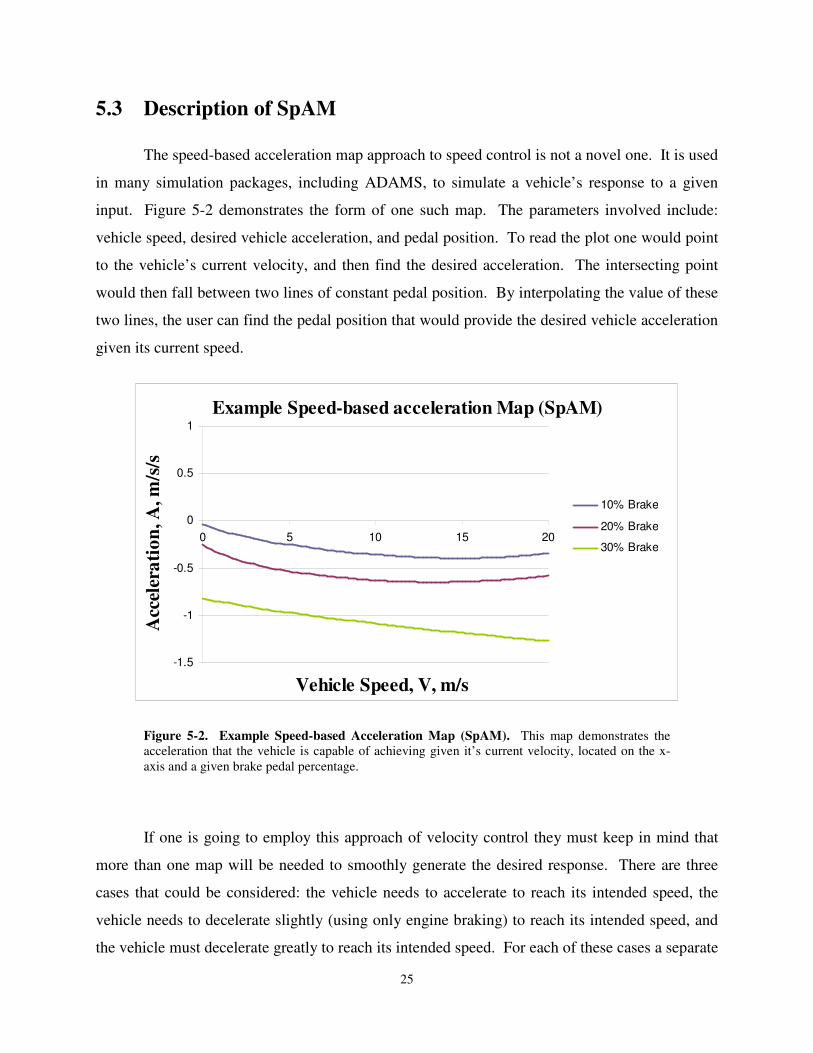
The speed-based acceleration map approach to speed control is not a novel one. It is used
in many simulation packages, including ADAMS, to simulate a vehicle’s response to a given
input. Figure 5-2 demonstrates the form of one such map. The parameters involved include:
vehicle speed, desired vehicle acceleration, and pedal position. To read the plot one would point
to the vehicle’s current velocity, and then find the desired acceleration. The intersecting point
would then fall between two lines of constant pedal position. By interpolating the value of these
two lines, the user can find the pedal position that would provide the desired vehicle acceleration
given its current speed.
Example Speed-based acceleration Map (SpAM)
-1.5
-1
-0.5
0
0.5
1
0 5 10 15 20
Vehicle Speed, V, m/s
Acc
eler
ati
on
, A
, m
/s/s
10% Brake
20% Brake
30% Brake
Figure 5-2. Example Speed-based Acceleration Map (SpAM). This map demonstrates the acceleration that the vehicle is capable of achieving given it’s current velocity, located on the x-axis and a given brake pedal percentage.
If one is going to employ this approach of velocity control they must keep in mind that
more than one map will be needed to smoothly generate the desired response. There are three
cases that could be considered: the vehicle needs to accelerate to reach its intended speed, the
vehicle needs to decelerate slightly (using only engine braking) to reach its intended speed, and
the vehicle must decelerate greatly to reach its intended speed. For each of these cases a separate
26
map must be generated and the governing algorithm must be able to choose between each map to
determine which is appropriate for use at the time.
For the development of this algorithm it was determined that although three maps would
be more accurate in predicting the correct pedal position, this was not necessary. A PID
controller would be used to correct for any error that was in the initial “guess” made by the feed
forward section of the loop, therefore simply getting within the “ballpark” of the correct pedal
position would be acceptable and would ease the creation of the algorithm.
Because the team did not have access to any mathematical models for the dynamics of
the vehicle, the curves for the map were obtained empirically.
5.3.1 Test to obtain the response of the vehicle
The data collected during this step was done at a rate of 20 Hz. The National Instruments
CompactRIO described earlier read and logged the vehicle’s speed from the vehicle’s onboard
CAN bus. The testing and data collection was done at a local drag racing strip. This location
was chosen because it was determined to be the longest stretch of flat, straight road available to
the team. The strip chosen had an eighth mile track with another eighth mile run out after the
finish line. The run out was created at an incline so as to aid in the slowing of a racer after they
crossed the line. This incline was not desirable for the team because the team was trying to
mitigate the affects of gravity. The incline was not a problem during acceleration tests because
the vehicle did not have a problem reaching the maximum desired speed, 50 mph, within the
eighth mile of flat course. However, there was not sufficient room for the vehicle to reach that
speed and then slow back to a stop while doing braking tests. The solution was run the course
backwards. By doing this, the incline would actually aid the vehicle to accelerate to the desired
speed more quickly, once the vehicle crossed the finish line and reached flat ground the
computer was given control of the brake and the correct pedal position was commanded.
Over twenty-two individual test runs were conducted during testing. The first eleven
tests were acceleration tests. From a stand still the vehicle speed was recorded while first
applying: zero throttle, 10% throttle, 20% throttle and so on until 100% throttle was reached.
27
The next set of eleven tests was brake testing. As mentioned, the course was run
backwards. The vehicle was brought up to 50 mph under manual control and then the computer
was given control. It first commanded: zero braking, 10% braking, 20% braking, and so on until
it reached 100% brake.
The final trials that were run were duplicates of each of the first throttle acceleration and
brake runs. By comparing the data collected from these runs with the earlier runs under the same
pedal percentages the team could verify that the methods used for pedal control were repeatable.
5.3.2 Processing the Data
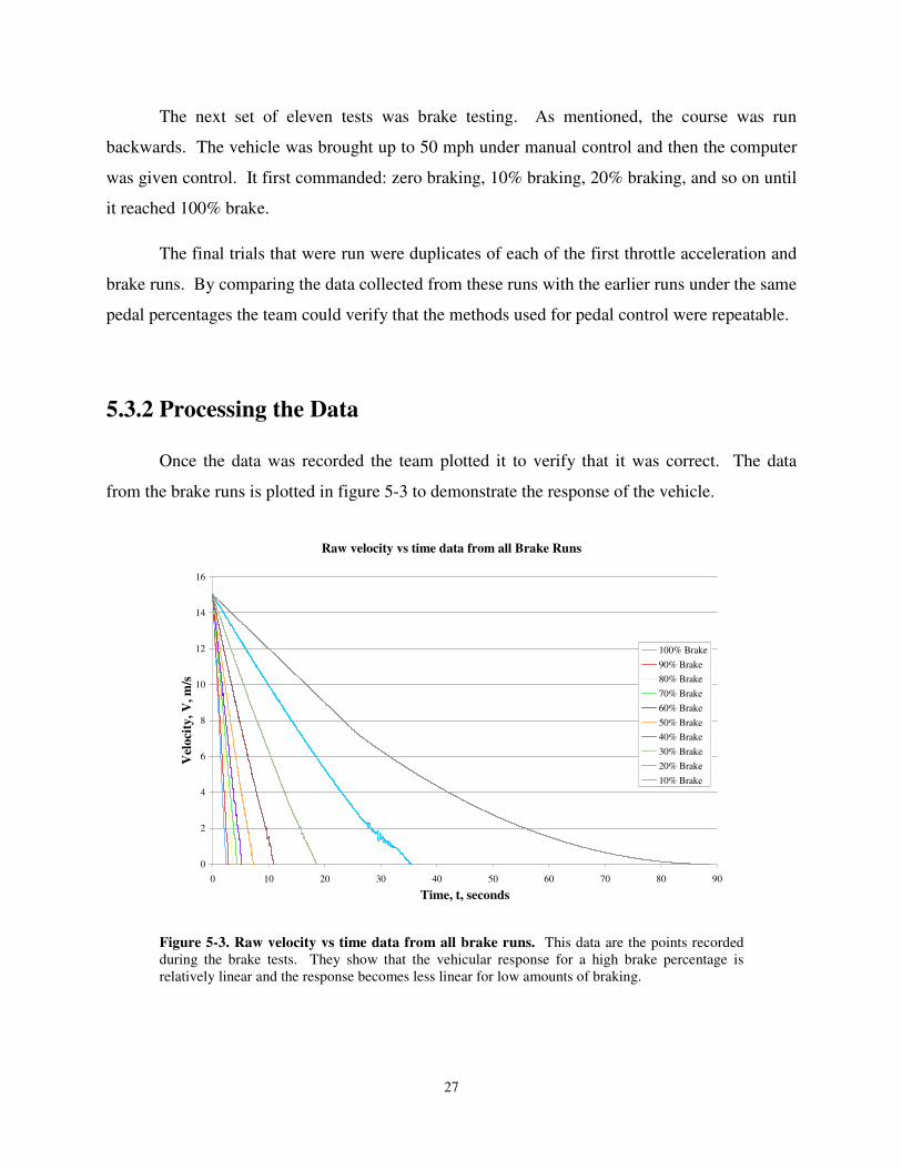
Once the data was recorded the team plotted it to verify that it was correct. The data
from the brake runs is plotted in figure 5-3 to demonstrate the response of the vehicle.
Raw velocity vs time data from all Brake Runs
0
2
4
6
8
10
12
14
16
0 10 20 30 40 50 60 70 80 90
Time, t, seconds
Vel
oci
ty,
V,
m/s
100% Brake
90% Brake
80% Brake
70% Brake
60% Brake
50% Brake
40% Brake
30% Brake
20% Brake
10% Brake
Figure 5-3. Raw velocity vs time data from all brake runs. This data are the points recorded during the brake tests. They show that the vehicular response for a high brake percentage is relatively linear and the response becomes less linear for low amounts of braking.
28
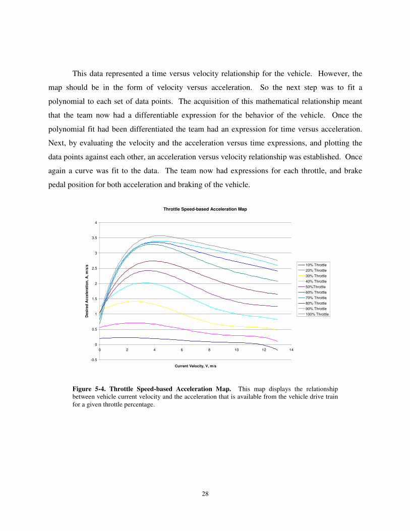
This data represented a time versus velocity relationship for the vehicle. However, the
map should be in the form of velocity versus acceleration. So the next step was to fit a
polynomial to each set of data points. The acquisition of this mathematical relationship meant
that the team now had a differentiable expression for the behavior of the vehicle. Once the
polynomial fit had been differentiated the team had an expression for time versus acceleration.
Next, by evaluating the velocity and the acceleration versus time expressions, and plotting the
data points against each other, an acceleration versus velocity relationship was established. Once
again a curve was fit to the data. The team now had expressions for each throttle, and brake
pedal position for both acceleration and braking of the vehicle.
Throttle Speed-based Acceleration Map
-0.5
0
0.5
1
1.5
2
2.5
3
3.5
4
0 2 4 6 8 10 12 14
Current Velocity, V, m/s
De
sir
ed
Ac
ce
lera
tio
n,
A, m
/s/s 10% Throttle
20% Throttle
30% Throttle
40% Throttle
50%Throttle
60% Throttle
70% Throttle
80% Throttle
90% Throttle
100% Throttle
Figure 5-4. Throttle Speed-based Acceleration Map. This map displays the relationship between vehicle current velocity and the acceleration that is available from the vehicle drive train for a given throttle percentage.
29
Braking Speed-based Acceleration Map
-9
-8
-7
-6
-5
-4
-3
-2
-1
0
0 2 4 6 8 10 12 14
Current Velocity, V, m/s
Des
ired
Ac
ce
lera
tio
n, A
, m
/s/s 10% Brake
20% Brake
30% Brake
40% Brake
50% Brake
60% Brake
70% Brake
80% Brake
90% Brake
100% Brake
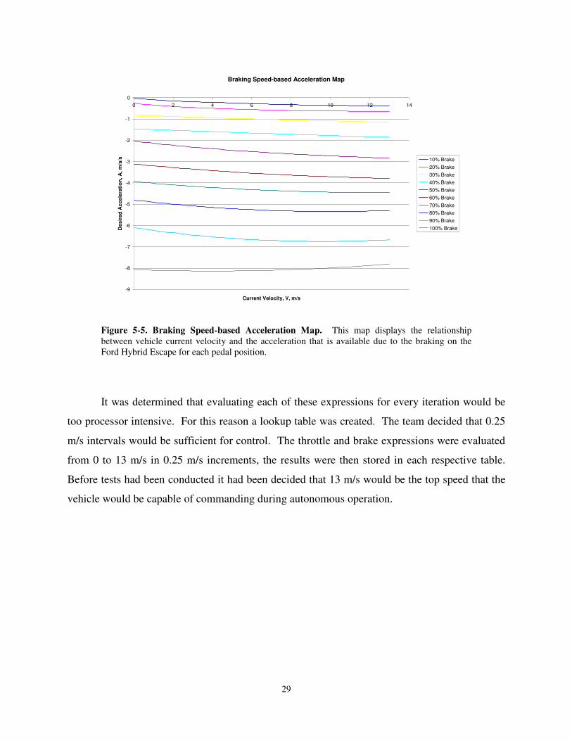
Figure 5-5. Braking Speed-based Acceleration Map. This map displays the relationship between vehicle current velocity and the acceleration that is available due to the braking on the Ford Hybrid Escape for each pedal position.
It was determined that evaluating each of these expressions for every iteration would be
too processor intensive. For this reason a lookup table was created. The team decided that 0.25
m/s intervals would be sufficient for control. The throttle and brake expressions were evaluated
from 0 to 13 m/s in 0.25 m/s increments, the results were then stored in each respective table.
Before tests had been conducted it had been decided that 13 m/s would be the top speed that the
vehicle would be capable of commanding during autonomous operation.
30
5.4 Implementation of SpAM
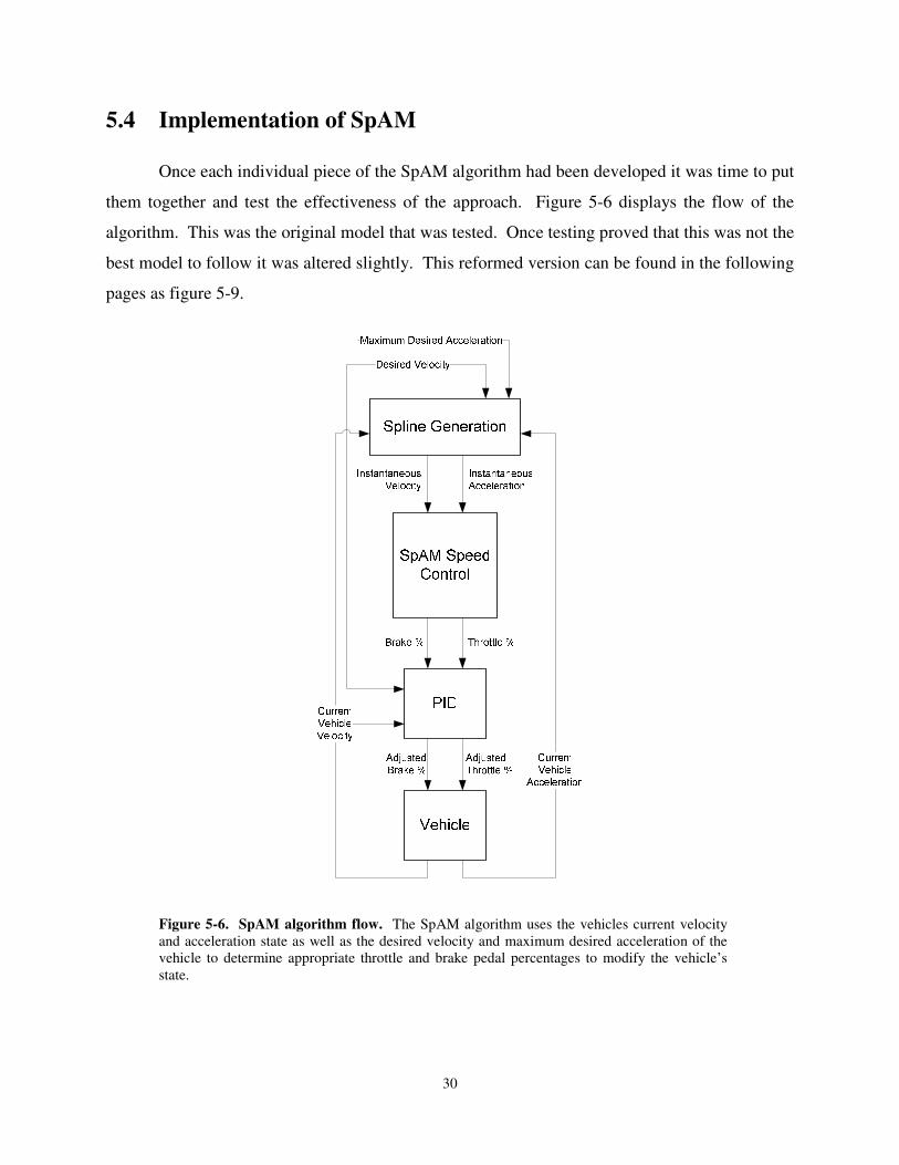
Once each individual piece of the SpAM algorithm had been developed it was time to put
them together and test the effectiveness of the approach. Figure 5-6 displays the flow of the
algorithm. This was the original model that was tested. Once testing proved that this was not the
best model to follow it was altered slightly. This reformed version can be found in the following
pages as figure 5-9.
Figure 5-6. SpAM algorithm flow. The SpAM algorithm uses the vehicles current velocity and acceleration state as well as the desired velocity and maximum desired acceleration of the vehicle to determine appropriate throttle and brake pedal percentages to modify the vehicle’s state.
31
There are four inputs into the algorithm: current velocity, current acceleration, maximum
desired acceleration, and desired velocity. The maximum desired acceleration determines the
slope of the first-order line generated by the spline generation algorithm. To this point it has
been stated that a PID controller is used in the final version of the software. In reality the
noisiness of the current velocity signal dictated that the derivative term of the PID caused the
system to go unstable. For this reason the derivative gain was zeroed and PI controllers were
implemented. A separate PI for each throttle and brake was used. The response of vehicle was
much smoother when the original single PI controller was split into two separate PI controllers.
The maximum desired acceleration is an unsigned number. The direction of the
acceleration is determined by comparing the desired speed to the current and determining if the
vehicle should accelerate or decelerate.
To test the effectiveness of the algorithm a flat stretch of road was used to perform three
evaluation runs. Each of these runs used a constant maximum desired acceleration, and the
desired velocity of 7 m/s was entered. Once the vehicle reached steady state the desired velocity
was reduced to 5 m/s. Again, when the response stopped changing the desired speed was
increased to 10 m/s. Lastly the desired velocity was set to 0 m/s. These values were chosen
because the test would encompass a range of typical speeds seen during operation as well
command a variety of positive and negative acceleration scenarios. The values of maximum
desired acceleration used for the tests were 0.75 m/s2, 1.5 m/s2 and 2.25 m/s2.
The responses for the system under the three different maximum accelerations varied. As
one would expect the responses varied in a predictable manner so the response for the 1.5 m/s2
run was a good average for the other two runs. The algorithm proved to be very accurate in
tracking vehicle acceleration. But it caused a high frequency oscillation while maintaining
speed. The algorithm was less accurate during times of negative acceleration but was still
acceptable.
32
Vehicle Response for SpAM and PI Controller Running at 1.5 m/s/s Amd
0
2
4
6
8
10
12
0 10 20 30 40 50 60 70 80
Time, t, seconds
Vel
oci
ty, v
, m
/sSpAM Vdes
SpAM Vact
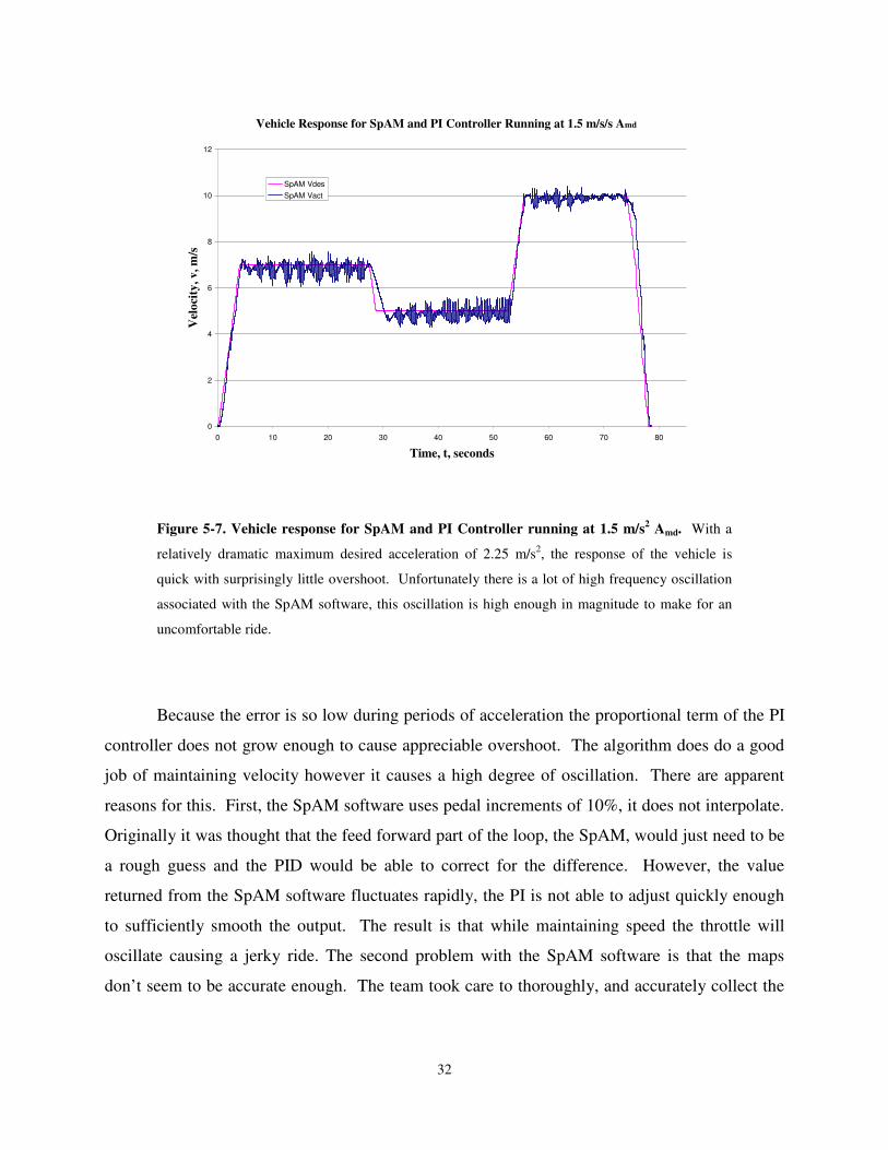
Figure 5-7. Vehicle response for SpAM and PI Controller running at 1.5 m/s2 Amd. With a
relatively dramatic maximum desired acceleration of 2.25 m/s2, the response of the vehicle is
quick with surprisingly little overshoot. Unfortunately there is a lot of high frequency oscillation
associated with the SpAM software, this oscillation is high enough in magnitude to make for an
uncomfortable ride.
Because the error is so low during periods of acceleration the proportional term of the PI
controller does not grow enough to cause appreciable overshoot. The algorithm does do a good
job of maintaining velocity however it causes a high degree of oscillation. There are apparent
reasons for this. First, the SpAM software uses pedal increments of 10%, it does not interpolate.
Originally it was thought that the feed forward part of the loop, the SpAM, would just need to be
a rough guess and the PID would be able to correct for the difference. However, the value
returned from the SpAM software fluctuates rapidly, the PI is not able to adjust quickly enough
to sufficiently smooth the output. The result is that while maintaining speed the throttle will
oscillate causing a jerky ride. The second problem with the SpAM software is that the maps
don’t seem to be accurate enough. The team took care to thoroughly, and accurately collect the
33
data needed to generate the maps. However, it seems that this approach is not resilient to
inaccuracies within the data.
To benchmark the response of the vehicle the three tests were repeated with the SpAM
algorithm turned off, only the PI controller was used. All of the same values for maximum
desired acceleration and desired velocities were used. The same stretch of road was run and the
approximate locations for changes in desired velocity were maintained throughout all tests.
The gain values used were the same that had been tuned using the full algorithm. A more
desired response could have possibly been obtained had some gain scheduling been employed
but the purpose of the test was to evaluate the effectiveness of the SpAM approach, not to design
a PID, or PI only controller.
Vehicle Response for PI Controller at 1.5 m/s/s Amd
0
2
4
6
8
10
12
0 10 20 30 40 50 60 70 80
Time, t, seconds
Velo
city
, v, m
/s
Actual Velocity
Desired Velocity
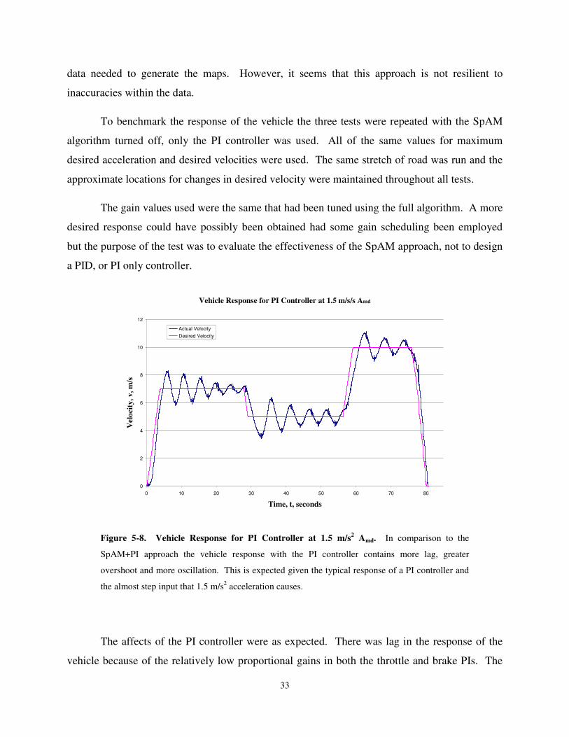
Figure 5-8. Vehicle Response for PI Controller at 1.5 m/s2 Amd. In comparison to the
SpAM+PI approach the vehicle response with the PI controller contains more lag, greater
overshoot and more oscillation. This is expected given the typical response of a PI controller and
the almost step input that 1.5 m/s2 acceleration causes.
The affects of the PI controller were as expected. There was lag in the response of the
vehicle because of the relatively low proportional gains in both the throttle and brake PIs. The
34
oscillation was limited because the low magnitude of the proportional gain but it was still
substantial. The response did not have time to settle before the desired velocity was changed.
This was dictated by the limited length of flat road that was available to run the test.
Because the SpAM software is not able to maintain speed comfortably, but produced
accurate acceleration profiles, little overshoot and quick settle time it was determined to be a
partial success. The area of control that was lacking was the speed maintenance. Because of this
the tests were once again conducted. This time however, the SpAM algorithm would only
contribute to the response of the vehicle when the instantaneous desired acceleration was not
equal to zero. When the vehicle was maintaining speed only the PI controller had control of the
throttle and brake. This decision led to a revised version of the preceding SpAM algorithm flow
chart. This revised version is seen in figure 5-9. This final version of the algorithm was dubbed
the “SpAM+PI” algorithm.
35
Spline Generation
Current
Vehicle
Velocity
Desired Velocity
Maximum Desired Acceleration
SpAM Speed
Control
PI
Vehicle
Instantaneous
Velocity
Throttle %
Throttle %Brake %
Instantaneous
Acceleration
Brake %
PI
Adjusted
Throttle %
Adjusted
Brake %
Current
Velocity
Desired
Velocity
Instantaneous
Velocity
Instantaneous
AccelerationMaintaining
Speed?
T
F
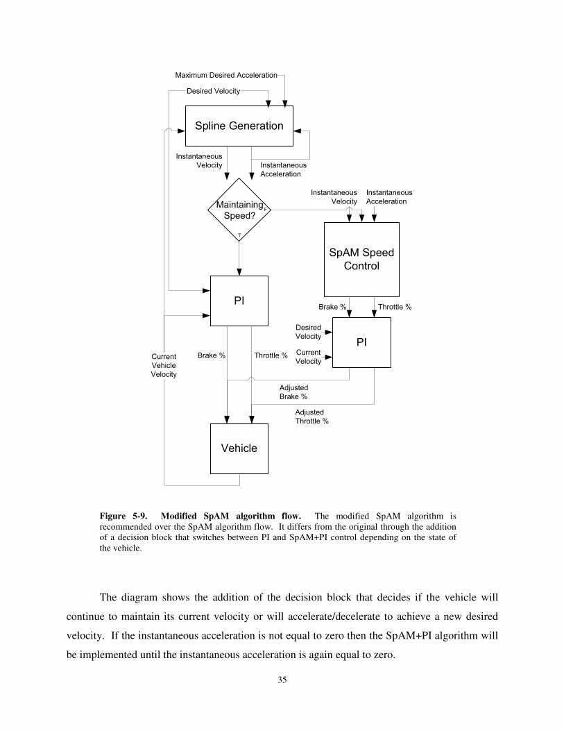
Figure 5-9. Modified SpAM algorithm flow. The modified SpAM algorithm is recommended over the SpAM algorithm flow. It differs from the original through the addition of a decision block that switches between PI and SpAM+PI control depending on the state of the vehicle.
The diagram shows the addition of the decision block that decides if the vehicle will
continue to maintain its current velocity or will accelerate/decelerate to achieve a new desired
velocity. If the instantaneous acceleration is not equal to zero then the SpAM+PI algorithm will
be implemented until the instantaneous acceleration is again equal to zero.
36
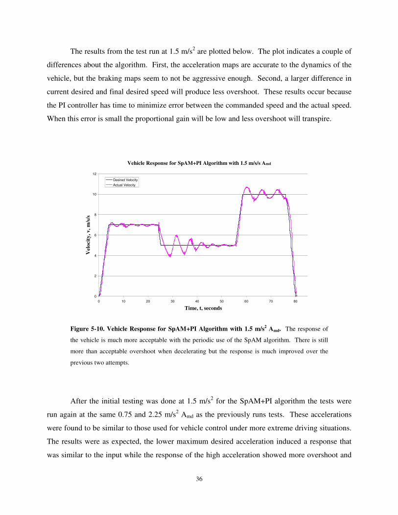
The results from the test run at 1.5 m/s2 are plotted below. The plot indicates a couple of
differences about the algorithm. First, the acceleration maps are accurate to the dynamics of the
vehicle, but the braking maps seem to not be aggressive enough. Second, a larger difference in
current desired and final desired speed will produce less overshoot. These results occur because
the PI controller has time to minimize error between the commanded speed and the actual speed.
When this error is small the proportional gain will be low and less overshoot will transpire.
Vehicle Response for SpAM+PI Algorithm with 1.5 m/s/s Amd
0
2
4
6
8
10
12
0 10 20 30 40 50 60 70 80
Time, t, seconds
Vel
oci
ty, v, m
/s/s
Desired Velocity
Actual Velocity
Figure 5-10. Vehicle Response for SpAM+PI Algorithm with 1.5 m/s2 Amd. The response of
the vehicle is much more acceptable with the periodic use of the SpAM algorithm. There is still
more than acceptable overshoot when decelerating but the response is much improved over the
previous two attempts.
After the initial testing was done at 1.5 m/s2 for the SpAM+PI algorithm the tests were
run again at the same 0.75 and 2.25 m/s2 Amd as the previously runs tests. These accelerations
were found to be similar to those used for vehicle control under more extreme driving situations.
The results were as expected, the lower maximum desired acceleration induced a response that
was similar to the input while the response of the high acceleration showed more overshoot and
37
slightly more lag. This lag was expected because the physical system could not react as
instantaneously as the desired commands; 2.25 m/s2 is a high acceleration for a fully laded
hybrid SUV.
Vehicle Response for SpAM+PI Algorithm with 0.75 m/s/s Amd
0
2
4
6
8
10
12
0 10 20 30 40 50 60
Time, t, seconds
Vel
oci
ty, v, m
/s
Desired Velocity
Actual Velocity
Figure 5-11. Vehicle Response for SpAM+PI Algorithm with 0.75 m/s2 Amd. At a lower
maximum desired acceleration the response is more desirable than at high accelerations. This
result is expected as the input to the PI is a shallower pitched ramp.
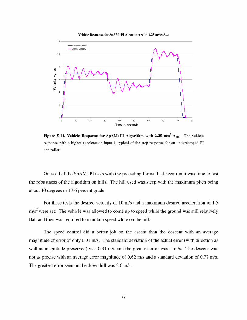
Although most aspects of the vehicle responses were expected, there was one that was
not. At 2.25 m/s2 acceleration the system was underdamped, meaning that the actual velocity
oscillated about the setpoint. In the trials run at 0.75 m/s2 the system showed no damping at all.
The steady state of the vehicle seemed to be a steady oscillation of significant amplitude. All of
these tests were run using the same gains and parameters for the controllers. The only difference
between runs was the desired maximum acceleration.
38
Vehicle Response for SpAM+PI Algorithm with 2.25 m/s/s Amd
0
2
4
6
8
10
12
0 10 20 30 40 50 60 70 80 90
Time, t, seconds
Vel
oci
ty, v, m
/s
Desired Velocity
Actual Velocity
Figure 5-12. Vehicle Response for SpAM+PI Algorithm with 2.25 m/s2 Amd. The vehicle
response with a higher acceleration input is typical of the step response for an underdamped PI
controller.
Once all of the SpAM+PI tests with the preceding format had been run it was time to test
the robustness of the algorithm on hills. The hill used was steep with the maximum pitch being
about 10 degrees or 17.6 percent grade.
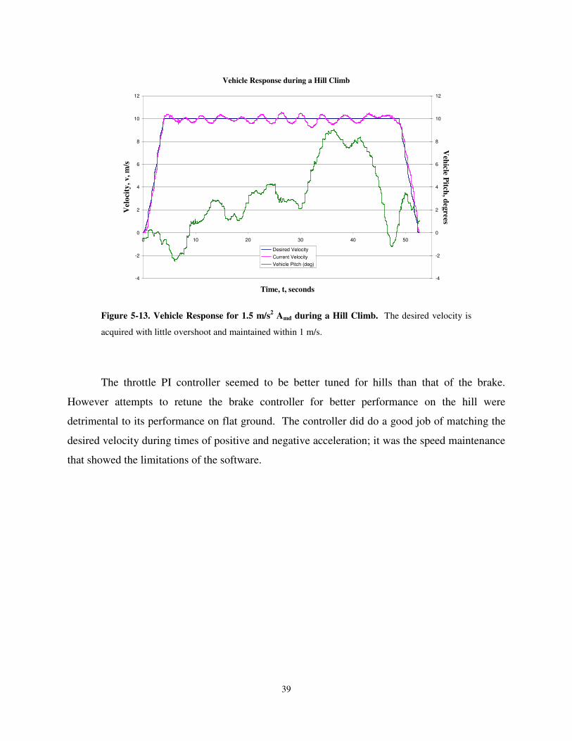
For these tests the desired velocity of 10 m/s and a maximum desired acceleration of 1.5
m/s2 were set. The vehicle was allowed to come up to speed while the ground was still relatively
flat, and then was required to maintain speed while on the hill.
The speed control did a better job on the ascent than the descent with an average
magnitude of error of only 0.01 m/s. The standard deviation of the actual error (with direction as
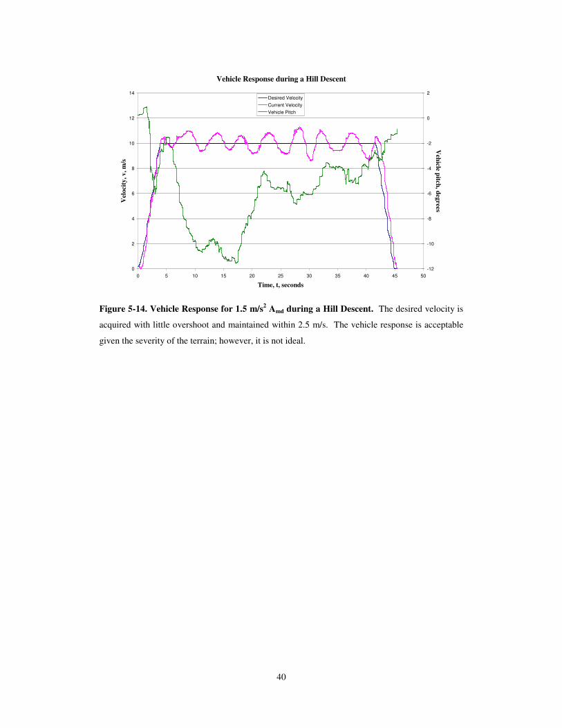
well as magnitude preserved) was 0.34 m/s and the greatest error was 1 m/s. The descent was
not as precise with an average error magnitude of 0.62 m/s and a standard deviation of 0.77 m/s.
The greatest error seen on the down hill was 2.6 m/s.
39
Vehicle Response during a Hill Climb
-4
-2
0
2
4
6
8
10
12
0 10 20 30 40 50
Time, t, seconds
Velo
city
, v,
m/s
-4
-2
0
2
4
6
8
10
12
Veh
icle
Pitc
h, d
egre
es
Desired Velocity
Current Velocity
Vehicle Pitch (deg)
Figure 5-13. Vehicle Response for 1.5 m/s2 Amd during a Hill Climb. The desired velocity is
acquired with little overshoot and maintained within 1 m/s.
The throttle PI controller seemed to be better tuned for hills than that of the brake.
However attempts to retune the brake controller for better performance on the hill were
detrimental to its performance on flat ground. The controller did do a good job of matching the
desired velocity during times of positive and negative acceleration; it was the speed maintenance
that showed the limitations of the software.
40
Vehicle Response during a Hill Descent
0
2
4
6
8
10
12
14
0 5 10 15 20 25 30 35 40 45 50
Time, t, seconds
Vel
oci
ty, v
, m
/s
-12
-10
-8
-6
-4
-2
0
2
Veh
icle pitch
, deg
rees
Desired Velocity
Current Velocity
Vehicle Pitch
Figure 5-14. Vehicle Response for 1.5 m/s2 Amd during a Hill Descent. The desired velocity is
acquired with little overshoot and maintained within 2.5 m/s. The vehicle response is acceptable
given the severity of the terrain; however, it is not ideal.
41
Chapter 6
Conclusions
The final implementation of the SpAM+PI approach is to run with only the PI
controller while maintaining speed and to integrate SpAM during times of desired speed change.
This configuration allows for a faster response time with less overshoot than a PI alone and a
smoother ride than continuous use of SpAM will provide.
While this SpAM+PI approach does show some promise, it was determined to be too
time and effort intensive to be practical. The generation of the speed maps is both time
consuming and sensitive to less than perfect data. In addition to the amount of time required to
generate the maps, some form of gain scheduling is still needed to handle the varieties of terrain
that the vehicle is likely to encounter.
42
6.1 Future Work
I would not recommend implementing the SpAM+PI approach for the speed control of a
full sized autonomous vehicle. The high amount of accuracy needed within the speed maps
means that a suitable test site of sufficient size is needed. This test site would allow the vehicle
to attain a speed greater than the maximum desired speed during operation, and then slow to a
stop using minimal braking. Also, any approach will need feedback to minimize error. The
conventional approach is to use a PID controller. It seems apparent that with a PID some amount
of gain scheduling will be needed to accommodate for inconsistent terrain. If the effort is going
to be made to create that gain scheduling scheme then it does not seem reasonable to also put
design effort into the development of the SpAM approach.
If a next attempt were to be made to design a speed control for the autonomous vehicle a
simple PI or PID would be used. This controller would have an extensive gain scheduling
scheme. The gains would be determined using the current error between the set point and
operating points, the desired acceleration, and the pitch of the vehicle. Ideally, the pitch of the
terrain in front of the vehicle would also be known so that the vehicle controller reaction could
preempt the response of the vehicle, just as a human driver would do.
and Hidetoshi Kato. “Development of the Hybrid/Battery ECU for the Toyota Hybrid
System.” Society of Automotive Engineers. Technical Paper 981122. 1998.
[7] Naranjo, Jose E.,Carlos Gonzalez, Ricardo Garcia, and Teresa de Pedro.
“ACC+Stop&Go Manuevers With Throttle and Brake Fuzzy Control.” IEEE
Transactions on Intelligent Transportation Systems Volume 7 (2006): 213-225
[8] Putney, Joseph. Reacitve Navigation of an Autonomous Ground Vehicle using Dynamic
Expanding Zones. Master’s Thesis, Virginia Tech, 2006.
[9] Reinholtz, Charles. DARPA Urban Challenge Technical Paper. Team Victor Tango.
(2007).
[10] Thurston, Robert H. A History of the Growth of the Steam Engine. New York: D.
Appleton and Company. 1878.
44
Appendix A: Testing Results
Vehicle Response for PI Controller with 0.75 m/s/s Amd
0
2
4
6
8
10
12
0 10 20 30 40 50 60
Time, t, seconds
Veh
icle
Vel
oci
ty,
v,
m/s
Desired Velocity
Actual Velocity
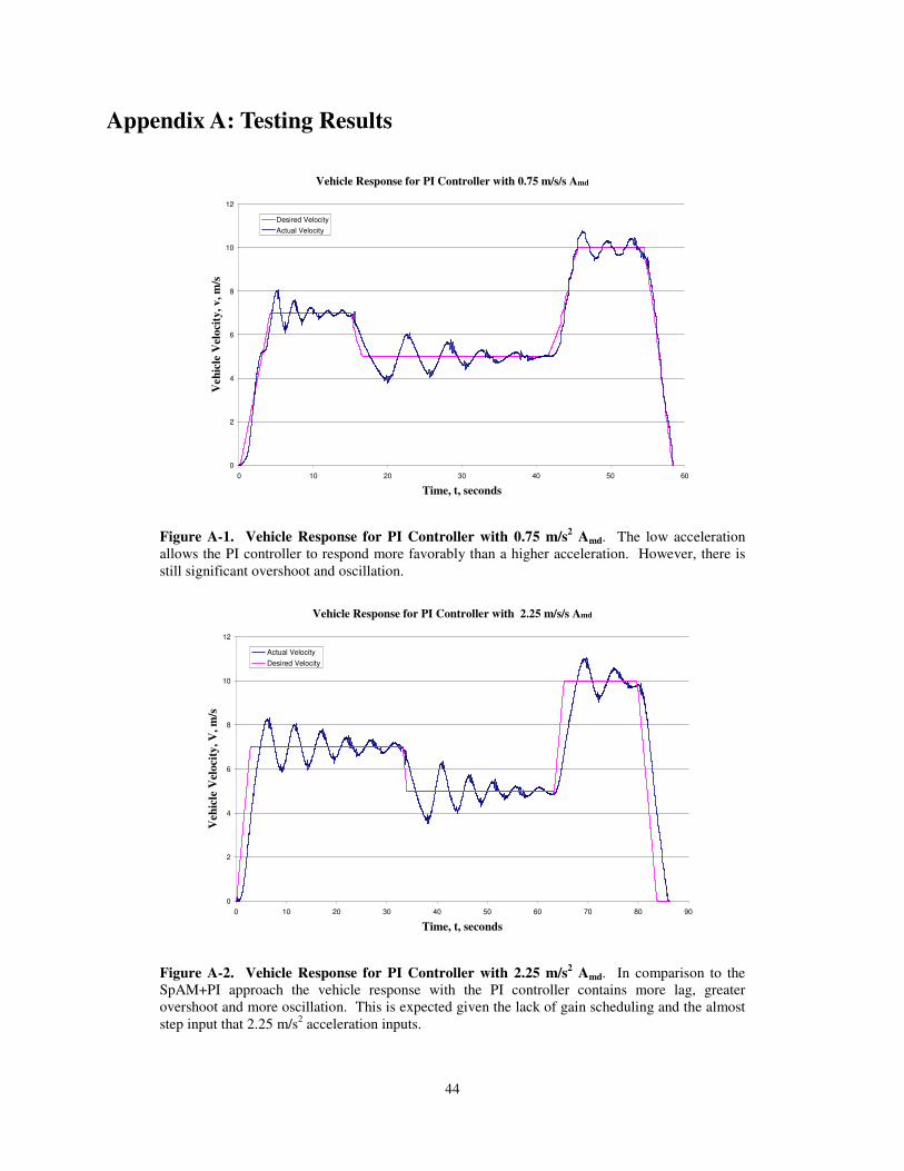
Figure A-1. Vehicle Response for PI Controller with 0.75 m/s2 Amd. The low acceleration
allows the PI controller to respond more favorably than a higher acceleration. However, there is still significant overshoot and oscillation.
Vehicle Response for PI Controller with 2.25 m/s/s Amd
0
2
4
6
8
10
12
0 10 20 30 40 50 60 70 80 90
Time, t, seconds
Veh
icle
Vel
ocit
y, V
, m
/s
Actual Velocity
Desired Velocity
Figure A-2. Vehicle Response for PI Controller with 2.25 m/s2 Amd. In comparison to the
SpAM+PI approach the vehicle response with the PI controller contains more lag, greater overshoot and more oscillation. This is expected given the lack of gain scheduling and the almost step input that 2.25 m/s2
acceleration inputs.
45
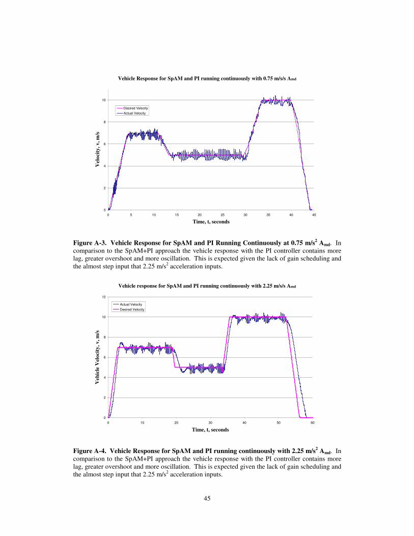
Vehicle Response for SpAM and PI running continuously with 0.75 m/s/s Amd
0
2
4
6
8
10
0 5 10 15 20 25 30 35 40 45
Time, t, seconds
Velo
city
, v, m
/s
Desired Velocity
Actual Velocity
Figure A-3. Vehicle Response for SpAM and PI Running Continuously at 0.75 m/s2 Amd. In
comparison to the SpAM+PI approach the vehicle response with the PI controller contains more lag, greater overshoot and more oscillation. This is expected given the lack of gain scheduling and the almost step input that 2.25 m/s2
acceleration inputs.
Vehicle response for SpAM and PI running continuously with 2.25 m/s/s Amd
0
2
4
6
8
10
12
0 10 20 30 40 50 60
Time, t, seconds
Veh
icle
Vel
oci
ty, v
, m
/s
Actual Velocity
Desired Velocity
Figure A-4. Vehicle Response for SpAM and PI running continuously with 2.25 m/s2 Amd. In
comparison to the SpAM+PI approach the vehicle response with the PI controller contains more lag, greater overshoot and more oscillation. This is expected given the lack of gain scheduling and the almost step input that 2.25 m/s2
acceleration inputs.
46
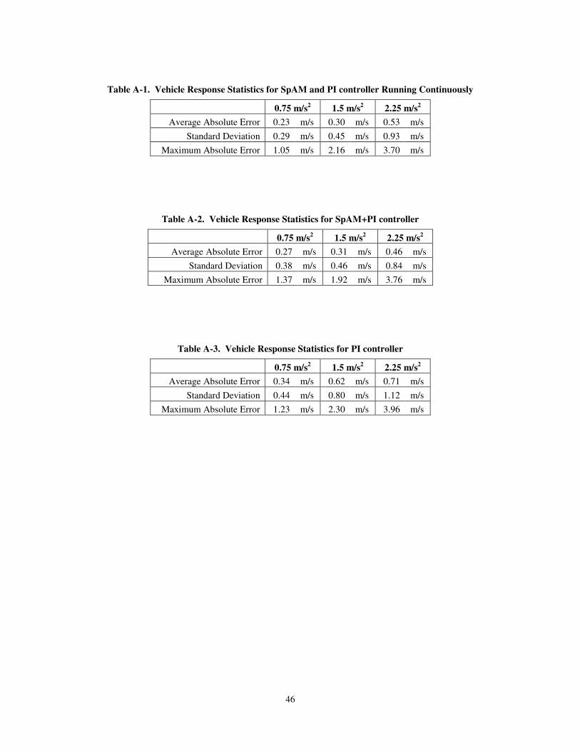
Table A-1. Vehicle Response Statistics for SpAM and PI controller Running Continuously
0.75 m/s2 1.5 m/s
2 2.25 m/s
2
Average Absolute Error 0.23 m/s 0.30 m/s 0.53 m/s
Standard Deviation 0.29 m/s 0.45 m/s 0.93 m/s
Maximum Absolute Error 1.05 m/s 2.16 m/s 3.70 m/s
Table A-2. Vehicle Response Statistics for SpAM+PI controller
0.75 m/s2 1.5 m/s
2 2.25 m/s
2
Average Absolute Error 0.27 m/s 0.31 m/s 0.46 m/s
Standard Deviation 0.38 m/s 0.46 m/s 0.84 m/s
Maximum Absolute Error 1.37 m/s 1.92 m/s 3.76 m/s
Table A-3. Vehicle Response Statistics for PI controller