28
Summary of Frequencies by Selvarasu A Mutharasu, Annamalai University 09-01-2-15 2:00 - 3:00 PM Lab II Nominal, Ordinal and Scale Data
| Date post: | 14-Jul-2015 |
| Category: |
Business |
| Upload: | mssstudents-shoppee-pvt-ltd-a-model-company |
| View: | 253 times |
| Download: | 2 times |

Summary of Frequenciesby Selvarasu A Mutharasu, Annamalai University09-01-2-15 2:00 - 3:00 PM Lab II
Nominal, Ordinal and Scale Data

You manage a team that sells computer hardware to software development companies. At each company, your representatives have a primary contact. You have categorized these contacts by the department of the company in which they work (Development, Computer Services, Finance, Other, Don't Know).This information is collected in contacts.sav. Use Frequencies to study the distribution of departments to see if it meshes with your goals.
Case Study 1: Summary of Frequencies

Choice of Summary of Frequencies
Nominal Data - Pie Chart, %, Count, Valid %
Ordinal Data - Bar Chart, Count, %, Cumulative, Valid %
Scale Data - Median, Mean, Quartiles, Skewness and Kurtosis

Operational Procedure for Summarizing the frequencies

Analyze Descriptive Frequencies

PIE CHART FOR NOMINAL DATA

Bar Chart for Ordinal Data
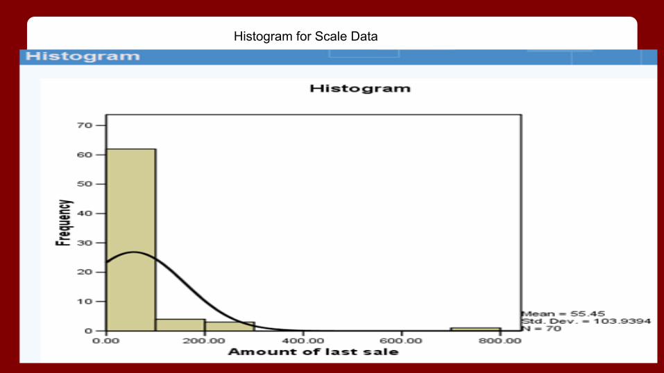
Histogram for Scale Data
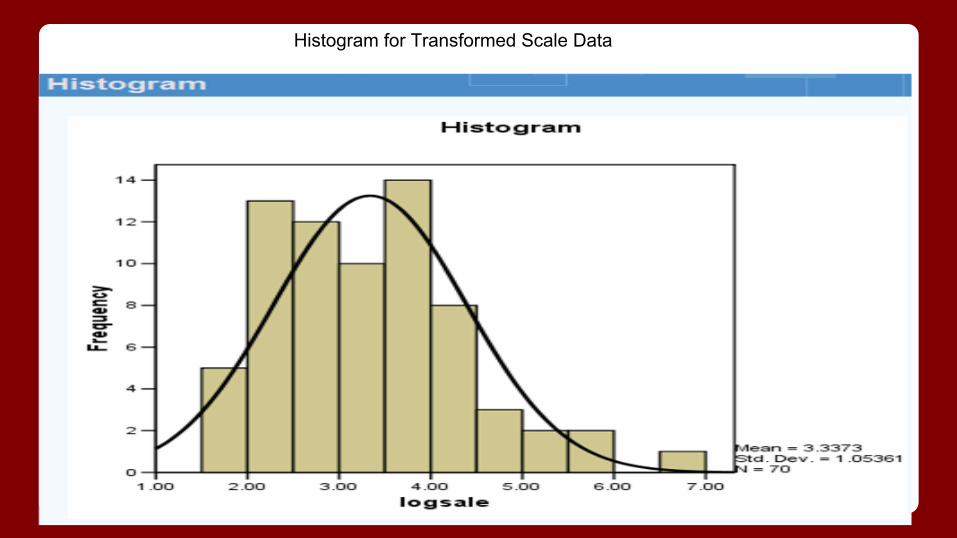
Histogram for Transformed Scale Data

Nominal Data - File Contacts.savTo run a Frequencies analysis, from the menus choose:
Analyze
Descriptive Statistics
Frequencies...
•Select Department as an analysis variable.
Categorize these contacts by the department of the company in which they work
–Development
–Computer Services
–Finance
–Other
Don't Know
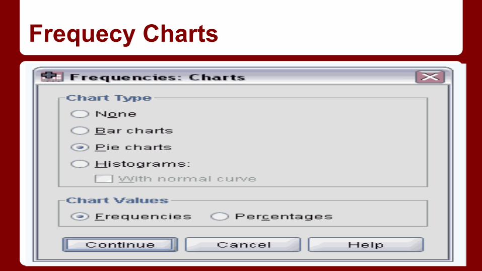
Frequecy Charts

Nominal Data Frequency Table

Ordinal Data Frequency Table
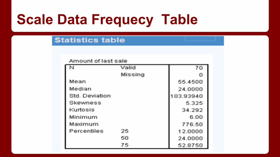
Scale Data Frequecy Table

InterpretationData assessment for Analysis

Nominal Data - Interpretation of Results
The Frequency column reports that 30 of contacts studied come from the computer services department. This is equivalent to 42.9% of the total number of contacts and 48.4% of the contacts whose departments are known. It is seen from the table that the departmental information is missing for 11.4% of contacts under study.

Ordinal Data - Procedure for summary frequency
► To summarize the company ranks of your contacts, from the menus choose:
Analyze
Descriptive Statistics
Frequencies...
► Select Company Rank as an analysis variable.
► Click Charts. ► Select Bar charts. ► Click Continue.
► Click Format in the Frequencies dialog box. ► Select Descending values. ► Click Continue. ► Click OK in the Frequencies dialog box.
•These selections produce a frequency table and bar chart with the categories ordered by descending value.

It is seen from the table that 15.7% of your contacts are junior managers. However, when studying ordinal data, the Cumulative Percent is much more useful. The table, since it has been ordered by descending values, shows that 62.7% of your contacts are of at least senior manager rank. As long as the ordering of values remains intact, reversed or not, the pattern in the bar chart contains information about the distribution of company ranks. The frequency of contacts increases from Employee to Sr. Manager, then decreases somewhat at VP, then drops off.
Ordinal Data - Interpretation of Results
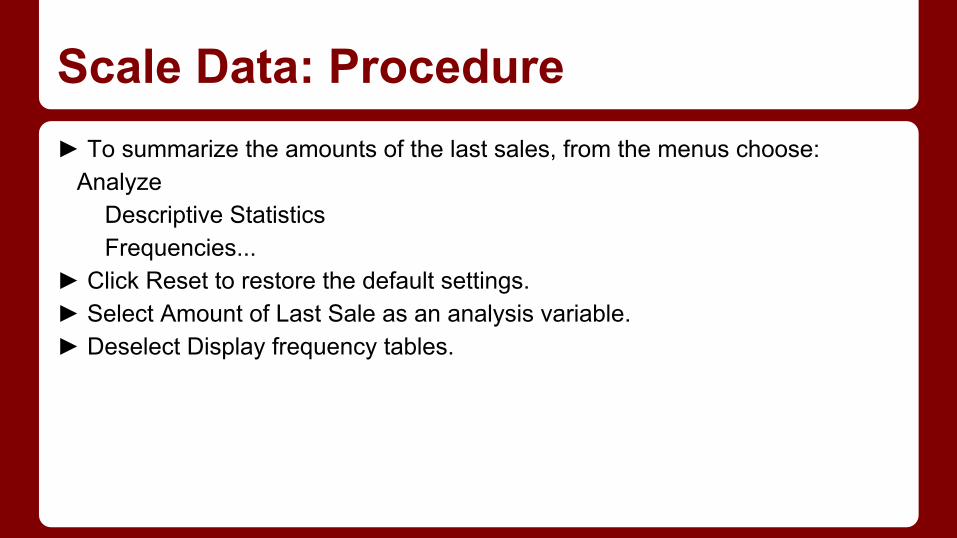
Scale Data: Procedure► To summarize the amounts of the last sales, from the menus choose: Analyze Descriptive Statistics Frequencies...► Click Reset to restore the default settings.► Select Amount of Last Sale as an analysis variable.► Deselect Display frequency tables.

Scale Data: Interpretation of Results
The center of the distribution can be approximated by the median (or second quartile) 24, and half of the data values fall between 12.0 and 52.875, the first and third quartiles. Also, the most extreme values are 6.0 and 776.5, the minimum and maximum. The mean is quite different from the median, suggesting that the distribution is asymmetric. This suspicion is confirmed by the large positive skewness, which shows that sale has a long right tail. That is, the distribution is asymmetric, with some distant values in a positive direction from the center of the distribution. Most variables with a finite lower limit (for example, 0) but no fixed upper limit tend to be positively skewed. The large positive skewness, in addition to skewing the mean to the right of the median, inflates the standard deviation to a point where it is no longer useful as a measure of the spread of data values. The large positive kurtosis tells you that the distribution of sale is more peaked and has heavier tails than the normal distribution.

Summarising Transformed Data● Many statistical procedures for quantitative data are
less reliable when the distribution of data values is markedly non-normal, as is the case with Amount of Last Sale.
● Sometimes, a transformation of the variable can bring the distribution of values closer to normal.

Procedure for Log Transformation To transform the variable sale, from the menus choose: Transform ► Compute Variable...► Type logsale as the Target Variable. ► Type LN(sale) as the Numeric Expression. ► Click OK.The log transformation is a sensible choice because Amount of Last Sale takes only positive values and is right skewed.

Procedure for Log Transformation Menu Screen

Transformed Data Summary

Transformed Table Scale Table

Graph: Histogram Transformed Data Scale Data

What is Histogram?
A histogram is a graphical representation of the distribution of data. It is an estimate of the probability distribution of a continuous variable (quantitative variable) and was first introduced by Karl Pearson.
Next Lesson...
Summary Statistics
using Descriptives
To study Quantitative Data...


