AIRCRAFT STABILITY DERIVATIVE ESTIMATION FROM FINITE ELEMENT ANALYSIS By DERIC AUSTIN BABCOCK Bachelor of Science Oklahoma State University Stillwater, Oklahoma 2002 Submitted to the Faculty of the Graduate College of Oklahoma State University in partial fulfillment of the requirements for the Degree of MASTER OF SCIENCE July, 2004
Transcript
AIRCRAFT STABILITY DERIVATIVE
ESTIMATION FROM FINITE
ELEMENT ANALYSIS
By
DERIC AUSTIN BABCOCK
Bachelor of Science
Oklahoma State University
Stillwater, Oklahoma
2002
Submitted to the Faculty of the Graduate College of Oklahoma State University
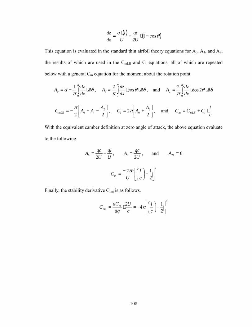
APPENDIX A: THIN AIRFOIL THEORY FOR CONSTANT PITCH RATE ............ 107
APPENDIX B: DATCOM CALCULATIONS FOR ISOLATED SURFACES ........... 109
APPENDIX C: DATCOM CALCULATIONS INCLUDING INTERFERENCE ........ 114
vi
LIST OF FIGURES
Figure 1.1: Illustration of Static Stability .......................................................................... 2 Figure 1.2: Illustration of Dynamic Stability..................................................................... 3 Figure 2.1: 3211 Multistep Applied to Velocity.............................................................. 16 Figure 2.2: Chirp Excitation Signal ................................................................................. 18 Figure 2.3: DC-Chirp Excitation Signal .......................................................................... 19 Figure 2.4: Longitudinal and Lateral Rigid Body Equations of Motion ......................... 22 Figure 2.5: Wagners Unsteady Lift ................................................................................ 24 Figure 3.1: The Effects of a Large Time Step on Excitation Signal................................ 37 Figure 3.2: Decoupling Position and Velocity Boundary Conditions ............................. 43 Figure 3.3: Geometry and Notation for Theodorsens Problem ...................................... 47 Figure 4.1: Geometry and Axis of Rotation for Horizontal Tail ..................................... 51 Figure 4.2: Grid Convergence Based on Moment Coefficient ........................................ 52 Figure 4.3: Close-up of Surface Grid for Horizontal Tail ............................................... 53 Figure 4.4: Pitch Rate and Angle of Attack (Alpha) for DC-Chirp................................. 55 Figure 4.5: Control File Parameters for Horizontal Tail.................................................. 56 Figure 4.6: Comparison of Cm for ARMA Model and STARS....................................... 57 Figure 4.7: Extraction of Stability Derivatives from the 35-14 ARMA Model............... 58 Figure 4.8: Stability Derivatives Extracted from the 29-49 ARMA Model .................... 59 Figure 4.9: Average Values of Stability Derivatives from Both Models ........................ 59 Figure 4.10: Comparison of Cm for Analytical and Quasi-Steady ARMA...................... 60 Figure 4.11: Comparison of Unsteady STARS to Quasi-Steady Analytical Results ...... 61 Figure 4.12: Geometry of Dihedral Wing........................................................................ 62 Figure 4.13: Longitudinal Grid Convergence.................................................................. 63 Figure 4.14: Lateral Grid Convergence ........................................................................... 64 Figure 4.15: Control File for Pitch Excitation ................................................................. 65 Figure 4.16: Resampled Pitch Moment Coefficient Time History with ARMA Model . 67 Figure 4.17: Comparison of Cm for Analytical and Quasi-Steady ARMA...................... 68 Figure 4.18: Geometry for Airfoil Test Case................................................................... 70 Figure 4.19: Pitch Moment Coefficient Due to Pitch Rate Only..................................... 72 Figure 4.20: Comparison of Pitch Damping Results for Airfoil Test Case ..................... 72 Figure 4.21: Pitch Damping Coefficient Versus Pitch Location ..................................... 73 Figure 4.22: A Closer Look at Pitch Damping Coefficient Versus Pitch Location......... 74 Figure 4.23: Pitch Moment Coefficient from Separate Excitation .................................. 77 Figure 4.24: Comparison of STARS Data and ARMA Model........................................ 78 Figure 4.25: Stability Derivatives Extracted from 23-21 ARMA Model ........................ 78 Figure 4.26: Pitch Moment Comparison of Simultaneous and Separate Excitation........ 79 Figure 4.27: Pitch Moment Comparison of Separate Excitation and Analytical............. 80 Figure 4.28: Rate Dependent Stability Derivative Estimates with Percent Differences.. 81 Figure 4.29: Pitch Moment Coefficient Versus Pitch Rate.............................................. 83
vii
Figure 4.30: Rate Dependent Stability Derivative Estimates with Percent Difference ... 84 Figure 4.31: Stability Derivative Estimate with Percent Difference ............................... 84 Figure 4.32: Geometry for Simplified Aircraft................................................................ 85 Figure 4.33: Dimensions of Simplified Aircraft .............................................................. 86 Figure 4.34: Stability Derivatives Estimated for Isolated Surfaces ................................. 87 Figure 4.35: Stability Derivatives Estimated for Simple Aircraft ................................... 88 Figure 4.36: Picture of the F-18sra Used in Flight Testing ............................................. 90 Figure 4.37: Picture of the F-18A Model Used in STARS.............................................. 91 Figure 4.38: Representative Control File for All F-18 Test Cases .................................. 92 Figure 4.39: Conditions Applied for the Estimation of Stability Derivatives ................. 93 Figure 4.40: Comparison of Flight Test Data to STARS Estimates for Cmα ................... 94 Figure 4.41: Comparison of Flight Test Data to STARS Estimates for Cmq ................... 95 Figure 4.42: Comparison of Flight Test Data to STARS Estimates for Clβ..................... 96 Figure 4.43: Comparison of Flight Test Data to STARS Estimates for Cnβ .................... 96 Figure 4.44: Comparison of Flight Test Data to STARS Estimates for Clp..................... 97 Figure 4.45: Comparison of Flight Test Data to STARS Estimates for Cnp .................... 97 Figure 4.46: Comparison of Flight Test Data to STARS Estimates for Clr ..................... 98 Figure 4.47: Comparison of Flight Test Data to STARS Estimates for Cnr .................... 98
viii
NOMENCLATURE
ARMA AutoRegressive Moving Average
b Wing Span
c Airfoil Chord
CASE Lab Computational AeroServoElasticity Laboratory
CFD Computational Fluid Dynamics
Cl Roll Moment Coefficient
Cm Pitch Moment Coefficient
Cn Yaw Moment Coefficient
Datcom United States Air Force Stability and Controls Datcom
displ Dimensionless Amplitude of Excitation Signal
FEA Finite Element Analysis
Ma Mach Number
MIMO Multi-Input Multi-Output
minpt Minimum Number of Points at Highest Frequency
NACA National Advisory Committee for Aeronautics
NASA National Aeronautics and Space Administration
na Number of Force Terms in Model
nb Number of Motion Terms in Model
np Number of Points for Identification
npt Number of Previous Terms
ix
nr Degrees of Freedom
over Overdetermination Factor
p Body-Fixed Roll Rate
psi Pounds per square inch
q Body-Fixed Pitch Rate
Q∞ Dynamic Pressure
r Body-Fixed Yaw Rate
RMS Root Mean Square
STARS STructural Analysis RoutineS
SVD Singular Value Decomposition
t Time
U Free Stream Velocity
u x-component of velocity
v y-component of velocity
Vmax Dimensionless Maximum Velocity of Excitation Signal
w z-component of velocity
α Angle of Attack
β Angle of Sideslip
θ Euler Pitch Angle
φ Euler Roll Angle
ρ Density
ω Angular Frequency / Sweep Frequency
ψ Euler Yaw Angle
1
CHAPTER 1
1INTRODUCTION
1.1 Background
Flight is a balancing act. For steady, level flight, all the forces and moments on
the aircraft must sum to zero; this is the equilibrium, or trim, condition. However, an
imbalance in forces must be created in order to maneuver the vehicle. If the aircraft
requires a large force to deviate from the reference position, it will be slow to respond to
pilot inputs. If instead, the vehicle requires little force to change course, then the pilot
must constantly correct for minor atmospheric disturbances. A balance must be struck
between resistance to disturbances and maneuverability.
The initial tendency of the system to return to equilibrium is termed static
stability. The classic representation of static stability can be seen in the three images of
Figure 1.1. A marble in equilibrium at the bottom of the bowl will initially try to return
to the bottom if the marble is moved then released, as seen in the top left image. This is a
statically stable system. In the top right image, the bowl is now inverted and the marble
is balanced at the top, any disturbance will cause the marble to diverge from the
equilibrium point, creating a statically unstable system. A statically neutral system is in
equilibrium at every position, with no preference to a particular position, as in the bottom
image.
2
Figure 1.1: Illustration of Static Stability
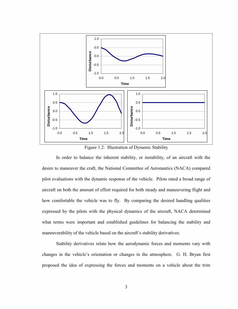
Dynamic stability is another matter. While the initial response defines the static
stability, the time history determines the dynamic stability. A system is dynamically
stable if the amplitude of the disturbance diminishes over time, as seen in the top image
of Figure 1.2. The amplitude of a disturbance in a dynamically unstable system grows
with time, as illustrated in the bottom left image. Finally, the bottom right image of
Figure 1.2 depicts a dynamically neutral system in which the amplitude remains constant.
It is important to note that a system can be statically stable but dynamically unstable. In
this case, the initial response may tend toward the equilibrium condition but overshoot
and not return. A dynamically stable system must be statically stable.
3
-1.0
-0.5
0.0
0.5
1.0
0.0 0.5 1.0 1.5 2.0
Time
Dis
turb
ance
-1.0
-0.5
0.0
0.5
1.0
0.0 0.5 1.0 1.5 2.0
Time
Dis
turb
ance
-1.0
-0.5
0.0
0.5
1.0
0.0 0.5 1.0 1.5 2.0
Time
Dis
turb
ance
Figure 1.2: Illustration of Dynamic Stability
In order to balance the inherent stability, or instability, of an aircraft with the
desire to maneuver the craft, the National Committee of Aeronautics (NACA) compared
pilot evaluations with the dynamic response of the vehicle. Pilots rated a broad range of
aircraft on both the amount of effort required for both steady and maneuvering flight and
how comfortable the vehicle was to fly. By comparing the desired handling qualities
expressed by the pilots with the physical dynamics of the aircraft, NACA determined
what terms were important and established guidelines for balancing the stability and
maneuverability of the vehicle based on the aircrafts stability derivatives.
Stability derivatives relate how the aerodynamic forces and moments vary with
changes in the vehicles orientation or changes in the atmosphere. G. H. Bryan first
proposed the idea of expressing the forces and moments on a vehicle about the trim
4
condition as a function of small perturbations from the trim condition [Nelson 1998]. For
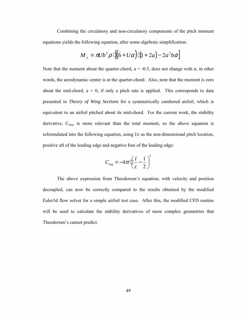
example, the change in pitch moment on an aircraft could be expressed as follows:
δδ
αα
∆⋅∂∂+∆⋅
∂∂+∆⋅
∂∂=∆ Mq
qMMM
The partial derivatives in the above equation are the stability derivatives. The problem
with this method is that the stability derivatives must be known before the model can be
used. Hence, stability derivative estimation is important for the evaluation of handling
quality and for the prediction of aerodynamic forces.
1.2 Motivation
The motivation for the current study is to reduce the time, costs, and restrictions
involved in the prediction of static and rate dependent stability derivatives. Calculating
stability derivatives typically means either making estimates from empirical data and
basic theory or conducting wind tunnel experiments and flight tests. Many of the
drawbacks of these methods can be eliminated through computational means, which are
becoming a more attractive alternative with the growing power and processing speed of
modern computers.
Analytical methods, such as those outlined in the USAF Stability and Control
Datcom [1978], are laden with assumptions and geometric restrictions as well as
limitations on the flight regime where the equations are applicable. Many of the methods
presented are empirical relations based on experiments. While the methods provided in
the Datcom yield insight into the dominant terms affecting the stability of an aircraft and
while this may be sufficient for the preliminary design process, more accurate results for
a broader range of geometries are desired.
5
Time and cost are the prominent disadvantages of experimental methods. The
long delay between a design decision and the results from an experiment prevent wind
tunnel testing from being an effective design tool in all but the most general cases. The
cost of constructing a model and testing facilities also deter the experimental method. If
design changes are made or modifications are needed, cost increases yet again. Wind
tunnel testing is most beneficial before flight-testing after the design is finalized. A
quicker, more cost efficient method is needed to determine the effects of decisions during
the design process.
In addition to safety hazards, flight-testing has many of the same drawbacks as
wind tunnel testing. If the behavior of the aircraft is not fully known for a given flight
regime, then a great deal of caution is needed to ensure the safety of the pilot. Correcting
stability and control problems is also more costly once the aircraft is built and ready for
testing than if the issues were discovered and resolved during the design process. Flight-
testing is a vital step in aircraft production, but with knowledge of how design decisions
will affect the stability and control of the aircraft, many problems can be avoided. With a
better understanding of the aircrafts response, flight-testing can be safer and more cost
efficient through the proper design of the experiment.
Improvements in the capabilities of computers and the robustness Computational
Fluid Dynamics (CFD) solvers are making computational methods more useful. Changes
in the design can be implemented easier in the computer model as opposed to a physical
model. The costs associated with CFD calculations are also much less than those of
experimental methods; and, reasonably accurate results can be obtained in a timeframe
suitable for the design process. Another benefit of a computational experiment is the
6
ability to exactly control the inputs and measure the outputs. A computer model can be
forced through oscillations that would be unsafe, or even impossible, for flight and wind
tunnel tests, but necessary for proper identification of the stability derivatives.
Furthermore, unlike empirical methods, CFD allows for the determination of stability
derivatives of an arbitrary geometry with a minimum of assumptions; however, since
CFD calculates forces through an integration of pressure, one must ensure that the
pressure is solved and integrated correctly for the given problem, and that the solution is
both grid and time-step converged.
1.3 Objective
The objective of this work is to investigate and implement an efficient procedure
for the accurate prediction of aircraft stability derivatives using finite element analysis
(FEA). This procedure should combine analytical, experimental, and computational
methods in order to retain the benefits of each while reducing the overall number of
limitations. The lessons and techniques learned through wind tunnel and flight tests, such
as excitation signals, model forms, and fitting procedures, will be applied in a
computational manner. The results of the computational experiments will then be used to
find and fit the best model to the data. Once the model has been found, analytical small-
disturbance theory will be used to extract the static and rate dependent stability
derivatives from the model. Alterations of the above procedure may be necessary in
order to maximize the benefits of the computational implementation, which is not limited
by the same constraints as experimental methods.
In order to achieve this end, the procedure should be able to calculate the stability
derivatives for an arbitrary geometry without any prior knowledge or estimates of the
7
values of the stability derivatives. Since most of todays high performance aircraft are
either unconventional or carry external stores, the method should not assume any
symmetry. Additionally, full advantage should be taken of any benefit that can be gained
through the computational implementation of this procedure, even at the expense of a
physically consistent motion as long as accuracy is maintained.
8
CHAPTER 2
2LITERATURE REVIEW
Estimating stability derivatives with the forced oscillation technique consists of
four main steps: exciting the system with a signal, recording the outputs of the flow
solver, fitting a model to the data, and finally extracting derivatives from the model. This
chapter presents the investigation into each of these steps and discusses the options that
best utilize the benefits of computational implementation.
2.1 Flow Solvers
The accuracy of a stability derivative estimate is dependent on the accuracy of the
forces calculated by the flow solver. The model is only as good as the data used to fit it.
Therefore, great care should be given to the proper selection of a flow solver. While
using a complex, all-encompassing CFD routine that can handle any flow regime or
phenomena would be computationally inefficient; the use of an inadequate solver is
futile. Due to the broad range of solvers available, this work is designed to be effective
with any solver. The forms of the input and output may be different, but the
methodology will be similar. To this end, the best solver is the one best suited for the
flow regime of interest.
2.1.1 General Requirements
For this effort, the desired solver should be accurate over a broad range of Mach
numbers and able to capture the flow physics relevant to general stability derivative
9
analysis. Because the emphasis is placed on regions where theory is incomplete or
unavailable, the solver should be capable of analyzing compressible fluid flow with and
without shockwaves. The effects of vortices and wake development are also important in
stability analysis, and should therefore be included. If a forced-oscillation technique is to
be used, the CFD routine must be able to calculate unsteady, time-dependent flows in a
non-inertial frame.
The inclusion of viscous effects greatly increases the computational requirements
and time costs of a numerical solution. While induced drag will be calculated properly
with the inviscid assumption, parasitic or form drag will not be. For stability derivative
determination, the values of the forces are not as important as the changes in the values of
the forces. If the drag calculations are incorrect by a constant, the derivatives will be
unaffected. In application, however, the inviscid assumption will affect the results to a
limited degree. Berry [1986] found the inclusion of viscosity into the CFD routine had
minimal impact on airfoil stability below the onset of stall. Therefore, to achieve the best
estimates of the stability derivatives, a viscous solver should be used; however, for this
research the effects of viscosity are neglected due to the time required to run a viscous
solution and the accuracy of the inviscid assumption. If the geometry or flow regime is
viscous dominated, a viscous solver may be appropriate, if not necessary. As such, these
flows are to be avoided when using an inviscid solver.
An example of a viscous dominated flow would be flow separation on smooth
bodies. Euler solvers can accurately model separation around sharp corners [Kandil
1990] due to the vortex domination of this type of separation. Boundary layer separation,
or stall, around smooth bodies such as wings or other aerodynamically shaped bodies is
10
viscous dominated. For the accurate estimation of stability derivatives in areas above
stall, viscosity effects must be included. However, as White [1991] stated, As long as
the angle of attack is below stall, the lift can be predicted by inviscid theory and the
friction by boundary-layer theory. While viscous solvers are limited by computational
expense, inviscid solvers are limited to flow regimes below the predicted onset of stall.
Although the current work is focused on rigid-body stability derivative extraction,
real aircraft are flexible. This flexibility can greatly alter the vehicles response. A
general solver should have the potential for incorporating elastic analysis. The control
derivatives may also need to be calculated. The ability to excite the control surfaces
while maintaining the aircraft at a fixed position would allow for the similar
identification of control derivatives. Likewise, the control derivative estimates could be
performed both with and without elasticity; therefore, a general solver should have
aeroservoelastic capability.
2.1.2 Panel Methods
Panel methods solve potential flows: flows that are incompressible, irrotational,
and inviscid. These numerical routines are typically quite computationally efficient
because they seek to define the boundary conditions on the body instead of solving for
the whole flow field [Katz 2001]. While corrections can be added to the routine in order
to account for compressibility and viscosity, they reduce the efficiency of panel methods;
the compressibility corrections can only correct for low Mach number compressibility
effects and cannot describe shock waves. If the reference flight condition were to have
local shocks, panel methods would be incapable of capturing these effects.
11
Another difficulty for complex geometries is the specifications of wake panels;
the location, shape, and strength of the wake panels must be specified for a unique
solution. As Katz [2001] states, [the wakes] geometry clearly affects the solution. To
properly model the wake would require some prior knowledge to the location, shape, and
strength of the wake. For low subsonic cases, a panel method may be adequate. Park
[1999] and Pesonen [2000] investigated panel methods without and with viscosity
corrections respectively, and achieved accurate results at and below a Mach number of
0.6. Compressibility corrections could not be accurately extended beyond this range.
Unfortunately, theory is limited to this range as well. In order to extend prediction
beyond the current limit on theory, a transonic solver is needed.
2.1.3 STARS
Developed at NASA Dryden Flight Research Center, STructural Analysis
RoutineS (STARS) integrates CFD, heat transfer, aeroservoelasticity, and both static and
dynamic structural routines for multidisciplinary design and analysis [Gupta 2001].
Euler3D, developed by Cowan [2003], can solve the unsteady Euler equations in a non-
inertial reference frame with a time-marching, finite element routine. Through rigorous
verification and validation with theoretical and experimental test cases, Euler3D has
demonstrated its ability to accurately capture the relevant flow physics.
In addition to the non-inertial motion specification, STARS is also capable of
simulating small amplitude motions through transpiration, which is well documented in
literature. Transpiration simulates motion by changing the normal vector to the surface
elements before applying the no-flow boundary conditions on wall elements. The surface
flow is then forced to travel perpendicular to the altered normal vector thereby
12
approximating the flow around a moving surface. Stephens [1998] discusses
transpiration further as well as the limits on the small amplitude assumption.
As an Euler solver, STARS can solve compressible, rotational flows over a broad
range of Mach numbers, but the flow must be inviscid. The wake issues of the panel
methods are minimized in this implementation as well. General knowledge of where
wakes will develop is still important for the proper distribution of elements, but shape
and strength issues are eliminated. Unlike panel methods, the STARS solution is
independent of the unnecessary elements that increase computational costs.
A drawback to this CFD routine is that FEA solves the flow at every node in the
flow field, not just surface nodes. The computational costs can become quite high for
large, complex cases. As with other inviscid solvers, STARS is limited to pre-stall flight
conditions. However, given the capability to achieve accurate results in the transonic
regime, the computational costs may be worthwhile.
2.1.4 Piston-Perturbation Solver
Hunter [1997] used piston theory to predict the aerodynamic forces on a body in a
supersonic flow. Piston theory relates the surface normal at a node on the body to the
surface pressure on that node. This simple relation bypasses a great deal of
computational work; however, it is not self-sufficient. For accurate results, the piston
theory must be applied about a reference condition, hence a piston perturbation method.
The perturbation pressure about the reference condition is a function of the steady state
pressure, and the change in the normal vector as seen in the following equation.
( )12
000 sin
211
−⋅
∞∞
−′⋅⋅−+⋅=
′ γγ
θθγ Mpp
pp
13
A finite-element Euler solver, such as STARS, is first used to compute the steady
state solution, and then the above equation calculates the pressure changes. This
extremely fast solution, as previously mentioned, is limited to the supersonic range, again
where adequate theory is typically available.
2.2 Excitation Signals
In order to determine the stability derivatives, the response of the aircraft to a
known input must be recorded. During forced-oscillation experiments, this input alone
controls the motion of the aircraft; the CFD solver simply calculates the forces and
moments acting on the body due to the motion. The signal, not the forces and moments,
dictate the motion of the aircraft. Numerous excitation signals are available, but the
signal must properly excite the correct terms. ONeill [2003] investigated various signals
for system identification of aeroelastic systems, and outlined the benefits of each signal.
However, these signals must be reevaluated based on the requirements for stability
derivative calculations instead of aeroelastic identification. The following section
outlines the requirements of the excitation signal. Various signals are then evaluated on
these criteria to determine the best form for the excitation signal.
2.2.1 Signal Requirements
The initial requirements of the excitation signal stem from the definition of
stability derivatives and the assumptions of small disturbance theory used to extract them
from the data. Namely, the vehicle must start at a steady flight condition, which requires
the signal to have a from-rest initial condition. Second, the stability derivatives are
assumed linear within small perturbations of the flight condition. The reference flight
14
condition may be in the nonlinear range, but the disturbances from this condition must be
in a local linear range. This requires that the signal be capable of fully exciting the
important terms to an acceptable degree while maintaining small displacements from the
reference condition. In flight-testing, designing an experiment that generates a pitch rate
large enough to accurately estimate the pitch damping term, Cmq, and keep the angle of
attack in the linear range is quite difficult [Klein 1998]. However, in a numerical
experiment, the pitch rate can be excited beyond the normal flight envelope for proper
identification, and the angle of attack maintained at minimal values.
A final intrinsic requirement of the excitation signal is that the boundary condition
specification must be physically consistent for a time accurate representation. For
instance, a step change in position would create an infinite velocity, distorting the
pressure calculations and the resulting forces and moments. However, a step change can
be used if only the steady or quasi-steady state response is desired; the solution is no
longer required to be time accurate.
Once a signal has met the above requirements, it may be judged further. In order
to generate data that can be used to train the model, the excitation of the input variables
must be seen in the output variables. If the input motions are excited in a manner that
produces little change in the output forces, some parameters will be unidentifiable and the
quality of the estimates of other parameters will be reduced [Klein 1998]. As a general
rule, if the user can see the effects of an input on the output when the response is plotted,
the routine which solves for the unknown parameters can as well. Klein also discovered
that exciting the system through control surfaces lowered the sensitivity of the outputs to
the inputs for parameter other than those associated with control derivatives. In a
15
computational implementation, the motion of the aircraft can be prescribed without using
control surfaces. This not only improves the sensitivity of the output but also reduces the
correlation of input variables; the effects of controls can be separated from the motion
effects. Iliff [1997] similarly concluded that the independent excitation of inputs yields
the best data for parameter identification.
In order to see the effect of the inputs, the excitation signal should contain
sufficient power at useful frequencies. Since steady and quasi-steady stability derivatives
are inherently low frequency, low-order terms, the power of the signal should be
concentrated over these lower frequencies. However, the range of important frequencies
is not clearly defined, so the power should be relatively constant over a sufficient range
of low frequencies to ensure that a reduction in power does not occur at important
frequencies.
Other implementation concerns include the ease with which the signal can be
specified. For instance, the specification of the maximum displacement or maximum
velocity should be intuitive, and the frequency range easily determined. Also of
importance is the robustness of the signal; one must determine whether small changes in
the description of the signal greatly alter the content of the signal. Because little may be
known about the aircraft response initially, the excitation signal should be somewhat
forgiving. The amount of work and computational resources required to implement a
signal must be considered as well. With these requirements in mind, the next section
describes the signals investigated for this study, and the results of that research.
16
2.2.2 Signal Characteristics
The following sections present each signal examined along with its advantages
and disadvantages. This discussion forms the knowledge base on which the appropriate
signal will be selected, and relies heavily on the results of ONeills thesis work [2003].
However, since the current effort is the identification of stability derivatives and not an
aeroservoelastic system, care must be taken in extrapolating from ONeills results.
2.2.3 3211 Multistep
The multistep, seen in Figure 2.1, is the standard signal for wind tunnel and flight-
testing experiments for numerous reasons. First, the signal is simple and easy for a pilot
to input. For a numerical implementation, a series of if-statements defines the signal.
Also, the multistep contains sufficient power at lower frequencies. The specification is
straightforward as well; the maximum displacement is the amplitude of the square wave.
-1.5
-1.0
-0.5
0.0
0.5
1.0
1.5
-2 0 2 4 6 8 10
Time
Dis
pla
cem
ent
-1.5
-1.0
-0.5
0.0
0.5
1.0
1.5
-2 0 2 4 6 8 10
Time
Vel
oci
ty
Figure 2.1: 3211 Multistep Applied to Velocity
While the 3211 has many benefits, the drawbacks are equally numerous. In
experiments, the multistep is typically applied to the displacement of control surfaces,
making the velocity and acceleration terms of little importance. Thus, the system can be
most fully excited by a full displacement of the control surface in alternating directions.
17
However, to use this signal in a forced-oscillation method, the multistep must be applied
to the velocity in order to maintain a physically consistent boundary condition as
discussed previously, see Figure 2.1. In this implementation, the velocity and
acceleration terms are more important, and not fully excited. The model, which is later
fitted to the data, will incorrectly account the nonphysical step change in velocity, leading
to further errors. Regular gaps in the power spectrum of the multistep also hinder the
chances of accurately exciting the necessary terms for the identification process.
2.2.4 Chirp
The chirp signal, seen in Figure 2.2, is in a class of signals that linearly sweep the
frequency range. By sweeping over a specified range of frequencies, the signal avoids
gaps in the power spectrum. In addition, the sinusoidal function excites the velocity and
acceleration terms. As seen in the following equations, displacement oscillates with the
same amplitude while the amplitude of velocity increases linearly with time and the
amplitude of acceleration increase with the square of time. Since the frequency increases
linearly with time, the specification of the frequency range is intuitively related to the
signal length.
( ) ( )2sin ttD ⋅= ω
( ) ( )2cos2 tttV ⋅⋅⋅⋅= ωω
( ) ( ) ( )2222 sin4cos2 ttttA ⋅⋅⋅⋅−⋅⋅⋅= ωωωω
Referring to the example given in Section 2.2.1, this signal allows for ample excitation of
pitch rate while maintaining a minimal angle of attack change. That the continuous
18
function specifies physically consistent boundary conditions with no step change is yet
another benefit to using a chirp signal.
-1.5
-1.0
-0.5
0.0
0.5
1.0
1.5
0.0 0.1 0.2 0.3 0.4 0.5 0.6 0.7 0.8 0.9 1.0
Time
Dis
plac
emen
t
-2.0
-1.5-1.0
-0.5
0.0
0.51.0
1.5
2.0
0.0 0.1 0.2 0.3 0.4 0.5 0.6 0.7 0.8 0.9 1.0
Time
Velo
city
Figure 2.2: Chirp Excitation Signal
The major disadvantage of the chirp is its lack of power at the lower frequencies.
While the amount of power over the lower range of frequencies is relatively constant, it is
still insufficient. For the proper identification of the aircraft stability derivatives, more
power must be applied in the low-frequency range. This is especially critical for the
displacement terms that tend to dominate the lower frequencies, as well as the velocity
terms that tend to dominate the higher frequencies.
19
2.2.5 DC-Chirp
The dc-chirp, seen in Figure 2.3, is very similar to the original chirp, and has
many of the same benefits. However, the dc-chirp differs in the offset, providing more
power in the displacement at lower frequencies. The defining equations for the dc-chirp
are as follows.
( ) ( )[ ]2cos121 ttD ⋅−⋅= ω
( ) ( )2sin tttV ⋅⋅⋅= ωω
( ) ( ) ( )2222 cos2sin ttttA ⋅⋅⋅⋅+⋅⋅= ωωωω
0.0
0.5
1.0
0.0 0.1 0.2 0.3 0.4 0.5 0.6 0.7 0.8 0.9 1.0
Time
Dis
plac
emen
t
-1.0
-0.5
0.0
0.5
1.0
0.0 0.1 0.2 0.3 0.4 0.5 0.6 0.7 0.8 0.9 1.0
Time
Velo
city
Figure 2.3: DC-Chirp Excitation Signal
20
As mentioned above, the offset of the dc-chirp improves the low frequency power
content for displacement. However, the velocitys low frequency power content is
unaffected. Since the lower frequencies are dominated by displacement terms, large
power content in the velocity terms would increase the correlation between the
displacement and velocity terms. The velocity terms become more important as the
frequency increases, and the dc-chirp provides adequate power at these frequencies. The
improved low frequency content comes at the expense of range. Since the offset moves
the centerline of the dc-chirp, only positive displacements are produced. To attain the
same amplitude as the original chirp, the dc-chirp would need twice the maximum value
of the original chirp, pushing the small perturbation limitations.
2.2.6 Other Signals
The Fresnel and Schroeder signals were also examined but dismissed based on
their failure to meet the minimum requirements. No closed form expression for the
Fresnel chirp requires a numerical integration, which can lead to a noisy input signal.
Any noise in the input can hinder the proper identification of the aircraft stability
derivatives. The Schroeder sweep has no inherit from-rest starting condition. Since the
stability derivatives are estimated about a reference condition, this signal must be adapted
to accept a from-rest initial condition. ONeill [2003] also found that the Schroeder
signal was excessively sensitive to excitation length.
21
2.3 Model Formulations
Once an accurate flow solver has generated the forces and moments resulting
from an appropriate excitation signal, a model can be used to describe the data set. The
parameters of this model reflect the trends and effects of the input on the output that are
not readily apparent in the raw data. If the model cannot accurately represent the data,
any stability derivatives extracted from the model will be inaccurate. Therefore, great
care must be given to the proper selection of a model form.
Klein [1998] describes a good model as one that sufficiently fits the data,
facilitates the successful estimation of unknown parameters whose existence can be
substantiated, and has good prediction capabilities. The model should therefore be
capable of fitting a broad range of data, contain parameters that realistically relate to
stability derivatives, and be accurate beyond the data used to fit the model.
22
2.3.1 Rigid Body Equations of Motion
The obvious equations for describing a vehicles dynamics are the aircraft
equations of motion presented in Figure 2.4 from Nelson [1998]. These equations are
derived from small disturbance theory and rigid body dynamics. Typically, they are
decoupled into longitudinal and lateral directions by making some general assumptions
about the moments of inertia. Because this model does not work explicitly with the
forced oscillation techniques previously mentioned, control surfaces or initial conditions
could be used to perturb the aircraft for measurement of the response. The direct
correlation of these equations to stability derivatives has made this method the standard
for flight-testing and wind tunnel experiments.
[ ]δ
θθδδ
δ
δ
∆⋅
++
∆∆∆∆
⋅
+++
−
=
∆∆∆∆
0010000
0
0
0
ZMMZX
qwu
uMMZMMZMMuZZ
gXX
qwu
wwqwwwuwu
wu
wu
&&&&
&&
&
&
∆∆
⋅
+
∆∆∆∆
⋅
⋅−
=
∆∆∆∆
ra
NLuY
NL
rp
NNNLLL
ug
uY
uY
uY
rp
r
r
r
a
a
rp
rp
rp
δδ
φ
βθ
φ
β
δ
δ
δ
δ
δ
β
β
β
00
0
001000
cos1
00
0
000
&
&
&
&
Figure 2.4: Longitudinal and Lateral Rigid Body Equations of Motion
The rigid body equations of motion are limited to steady or quasi-steady flows;
they do not account for the unsteady terms in the aerodynamic forces that will inevitably
occur due to the motion of the vehicle. The excitation required to accurately identify the
rate-dependent stability derivatives also excites higher order terms. In addition, the
difficulty of this model is increased when the simplifying assumptions no longer held.
For example, if the aircraft has an external store beneath one wing but not the other, or if
23
the geometry is unconventional, the equations cannot be decoupled into longitudinal and
lateral directions.
2.3.2 Indicial Functions
The indicial approach represents the forces or moments as a superposition of steps
with varying amplitude. With smaller and smaller time steps, the indicial model
approaches a continuous function. Klein [1997] demonstrated how the indicial function
could be used to determine the stability derivatives through the integral term that models
the unsteady wake effects. The following equation is the unsteady lift coefficient in
indicial function form about a reference condition, as given by Klein.
( ) ( ) ( )∫∫ +⋅⋅−⋅+⋅⋅−=t
Lq
t
LL dqddtC
Vld
ddtCtC
00
...ττ
ττατ
τα
The ellipsis was added to this equation in order to convey other terms that might be
necessary for a different configuration. In the same paper, Klein also presented the
following form for the time variant CL term, while assuming pitch-acceleration was
negligible.
( ) ( ) ceatC tbL +−= ⋅1α
24
In the above equation, the change in lift coefficient with respect to angle of attack
asymptotically approaches the quasi-steady value from some initial value. This
formulation correlates with Wagners unsteady lift problem, seen in Figure 2.5, with the
lift initially at one-half the final steady state value.
0.0
0.2
0.4
0.6
0.8
1.0
0 2 4 6 8 10 12 14 16 18 20
Non-Dimensional Time
CL(
t)/CL
Figure 2.5: Wagners Unsteady Lift
However, the indicial approach fails to correctly identify the stability derivatives
when the assumed form is no longer valid. In some cases, the effects of the wake may
not diminish exponentially. For example, the effect of the wake shed from the wing will
have a decreasing influence on the aircraft forces until the wake begins to interact with
the tail surfaces. The vehicle investigated in Kleins 1997 paper had a trapezoidal wing,
with no surfaces aft of the wings trailing edge. Another difficulty lies in the integro-
differential form of the equations, leading to further problems identifying model
parameters [Gupta 1985].
25
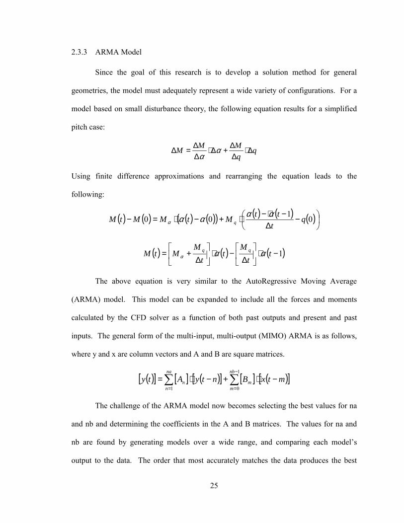
2.3.3 ARMA Model
Since the goal of this research is to develop a solution method for general
geometries, the model must adequately represent a wide variety of configurations. For a
model based on small disturbance theory, the following equation results for a simplified
pitch case:
qqMMM ∆⋅
∆∆+∆⋅
∆∆=∆ α
α
Using finite difference approximations and rearranging the equation leads to the
following:
( ) ( ) ( ) ( )( ) ( ) ( ) ( )
−
∆−⋅−⋅+−⋅=− 0100 q
tttMtMMtM q
ααααα
( ) ( ) ( )1−⋅
∆
−⋅
∆
+= tt
Mt
tM
MtM qq ααα
The above equation is very similar to the AutoRegressive Moving Average
(ARMA) model. This model can be expanded to include all the forces and moments
calculated by the CFD solver as a function of both past outputs and present and past
inputs. The general form of the multi-input, multi-output (MIMO) ARMA is as follows,
where y and x are column vectors and A and B are square matrices.
( )[ ] [ ] ( )[ ] [ ] ( )[ ]∑ ∑=
−
=
−⋅+−⋅=na
n
nb
mmn mtxBntyAty
1
1
0
The challenge of the ARMA model now becomes selecting the best values for na
and nb and determining the coefficients in the A and B matrices. The values for na and
nb are found by generating models over a wide range, and comparing each models
output to the data. The order that most accurately matches the data produces the best
26
model. Several criteria can be used to determine the best match to the data, including the
RMS of the error or cross correlation. If the model order does not converge, the range
must be expanded. Once the best model has been found, the stability derivatives can be
extracted from the coefficients in the model.
The ARMA model has been used successfully with the Euler flow solver in
STARS to accurately model aeroservoelasticity over a broad range of configurations and
flow regimes [Cowan 1995, Boeckman 2003, and ONeill 2003]. The flexibility and
accuracy of the ARMA model that is evident from the aeroservoelastic research could be
very beneficial in stability derivative extraction. For stability derivative analysis, the
inputs of the model would be rigid body rotations and displacements, instead of structural
mode displacements as with the aeroelastic case.
Hollkamp [1991] and Hamel [1996] applied the ARMA model to flight-test data
with limited success. Unfortunately, the noise inherent in measurement and signal
generation for a physical system is a small disturbance, which the ARMA model will try
to capture. In a strictly computational implementation, neither of these problems should
occur, as long as the signal excites the appropriate terms, the model is valid, and the CFD
solver calculates the forces properly.
2.3.4 Nonlinear Model: Stepwise Regression
Stepwise regression is very similar to the ARMA model of the previous section.
Like ARMA, this model calculates forces and moments as linear sums of the state
variables; however, stepwise regression does not incorporate any past inputs or outputs.
Instead, the unsteady effects are modeled by nonlinear combinations of states, such as α2
or αβ. The general identification process proceeds as follows: First, one must establish a
27
set of terms that might enter the model and fit the best linear model to the data. Next, the
significance of each term is evaluated, retaining only the influential terms for the next
step. Once a linear model with only the significant terms is achieved, then the nonlinear
terms are added one at a time. The significance of each parameter is checked after each
term is added with only dominant terms remaining.
While promising, this model has severe limitations, the primary one being that the
nonlinear terms do not provide insight into the stability derivatives. Worse still,
nonlinear terms could de-emphasize real linear terms in favor of unsubstantiated
nonlinear terms. Even though only the significant terms are to remain in the model,
Klein [1998] states, from experience, the model can still include too many terms and
have poor prediction capabilities. Another problem lies in the specification of which
terms should enter the model. While the number of combinations can be reduced through
engineering judgment, important terms can still be overlooked.
Nonlinear models may not be necessary. Klein [1998] found that linear models
were acceptable at low angles of attack, those less than 40 degrees. At high angles of
attack, separation occurs; therefore, an Euler flow solver could not properly calculate the
forces in this flow regime. Kleins conclusion about nonlinear models agrees with
Dowells [1995] assessment that aerodynamic calculations using a linear model about a
nonlinear condition, such as a shock wave, are sufficiently accurate. As such, nonlinear
models, in general, may be ruled out as a possibility for stability derivative extraction.
2.4 Parameter Estimation Methods
Once the model form is selected, parameter estimation involves the process of
determining the unknown parameters in that model from its input and output data.
28
Numerous, well-developed methods are available for fitting a curve to data; selecting the
most appropriate one depends on the type of data and model. To this end, the following
text briefly outlines the most common methods and the types of models for which they
are best suited. The appropriate estimation method then results from the type of model
and data, and is not a completely independent choice.
2.4.1 Maximum Likelihood Estimation
The most common parameter estimation method for fitting a model to flight-test
data is a maximum likelihood estimator. This approach seeks to maximize the
probability that the model will equal the measured data given a parameter value,
requiring a priori estimates. Typically used with the rigid body equations of motion, the
maximum likelihood method filters noise in both the input and output, including
measurement noise. The unsteadiness is thus filtered by assuming the effects to be
Gaussian white noise; however, unsteady terms are not random and can be far from
white [Klein 1998]. Analysis of maneuvers containing unsteady transonic flow or
inertial coupling of the longitudinal and lateral directions was more prone to failure [Iliff
1976].
2.4.2 Output Error Method
If no noise is present in the input, the above method simplifies to an output error
method, or a Newton-Raphson method. The output error method is typically used in
wind tunnel experiments where the inputs can be controlled more accurately than in flight
tests. While this simplification eliminates the need for a priori values, output error
methods still assume that the unsteady effects (the difference between the steady state
29
model and the unsteady data) are Gaussian white, and, as stated above, this is not always
the case. If a model includes unsteady terms such that the difference in the model and the
data is due only to measurement noise, then the output error approach is appropriate.
However, in computational implementation, further simplifications can be made.
2.4.3 Equation Error Method
With the added assumption that the output is measured without noise, the output
error method becomes the equation error method. Now that the states are measured
exactly, the unsteady effects on the output are not filtered or minimized. The model must
now account for the unsteady terms for the models output to match the data in order to
minimize the error. This method is so appealing it has been applied to data even when
the assumptions are not valid in order to obtain initial values for the Maximum
Likelihood estimator. Klein [1998] listed the main benefits of the equation error method
as follows: It is a simple non-iterative method; it provides starting values for other
methods; it can use partitioned data; and, it can aide in model structure determination.
The actual implementation of the equation error method to estimate the best
parameters in a least squares sense can be done by Singular Value Decomposition (SVD).
While SVD is more robust than other methods that typically fail due to data collinearity
[Klein 1998] or very small pivot elements [Cowan 1998], less dominate terms are forced
to zero in order to preserve stability. This can cause problems when trying to identify a
small parameter, such as pitch damping, which has a small overall effect on force but is
nonetheless an important damping term. SVD is a tool to be used in the process of
identifying model parameters, therefore its development has been omitted in order to
maintain focus on issues more relevant to the current work.
30
CHAPTER 3
3METHODOLOGY
The following sections outline two methods for the estimation of stability
derivatives: forced oscillation parameter identification and decoupled boundary
condition specification. First, each step of the forced oscillation parameter identification
exciting the system, recording the response, identifying the model, and extracting the
stability derivatives is described in detail. Next, a discussion about decoupling the
velocity and position boundary conditions is presented, as well as the derivation of a new
boundary condition equation. In a similar manner, Theodorsens equation will be
reexamined in order to produce theoretical values for comparison to initial testing of the
decoupled boundary condition method.
3.1 Forced Oscillation Parameter Identification
The objective for this section is to implement a computational forced oscillation
technique in order to determine stability derivatives, and refine the process to take full
advantage of the benefits of the CFD solver. To this end, the STARS flow solver,
Euler3d, is used to calculate the forces and moments on the body resulting from the dc-
chirp excitation signal. The data is then fit to an ARMA model with the stability
derivatives extracted from coefficients of the model. The following sections describe the
implementation of the stability derivative extraction technique.
31
3.1.1 CFD Solver
As stated previously, the CFD routine implemented in this research is Euler3d,
which is an Euler flow solver capable of calculating compressible, inviscid flow over a
broad range of Mach numbers from subsonic to supersonic in a non-inertial frame as well
as through transpiration for smaller motions. For a more complete description of the
implementation of STARS and Euler3d, the reader is referred to Gupta [2001] and
Cowan [2003], respectively.
While the flow parameters, such as Mach number, time step, dissipation model,
and solver order, are governed by the control file, the non-inertial motion of the system is
controlled through the dynamic file. Since the zero order, steady state solver was
developed assuming a physically consistent position and velocity relation, this solver
cannot account for non-inertial motion. At the very least, a first-order, time-accurate
solver must be specified in the control file when implementing the non-inertial motion
specification. The first order solver requires more computational time at each time step,
causing the non-inertial formulation to operate more slowly than a method based on a
steady solver. When the use of non-inertial motion is specified in the control file, the
dynamic output file contains the position, velocity, and acceleration of all six degrees of
freedom at every time step.
Information relevant to the current work, contained in the dynamic file, includes
the vector to the origin of rotation, the initial orientation and velocity, if any, and the type
of excitation. The origin of rotation is also the location of the force and moment
calculations in the non-inertial formulation; otherwise, the origin of the grid coordinate
serves as the force and moment reference. For standard aircraft coordinates, a ψ angle of
32
180 degrees is specified because STARS assumes the flow travels in the positive x-
direction. When a non-inertial file is implemented, the flow angles in the control file are
not used by STARS and must be adjusted in the dynamic file. If stability derivative
estimates are desired about an angle of attack or sideslip, then the base angles can be
entered as an initial condition in the dynamic file and the dc-chirp signal can excite the
system around that condition for a given excitation type. For the independent excitation
type, either velocity or position can be held at the initial value while the other is excited.
A different excitation type, the decoupled boundary condition specification, holds the
initial position and velocity constant; even for a non-zero velocity, position is held
constant. The decoupled excitation types require a modification to the acceleration
equation as discussed in Section3.2.2 on page 45.
As previously discussed, transpiration simulates motion by altering the normal
vector of a surface. Flow tangency is then applied to the surface defined by the new
normal vector accurately modeling the actual flow for small changes in the normal
vector. In order to apply transpiration to stability derivative analysis, a vector file
defining the mode shapes in terms of the rigid body degrees of freedom must be
generated about the origin of simulated rotation. The vector file contains the initial
conditions, the excitation type, and the mode shape definition. Again, the excitation
types include: dc-chirp excitation about the initial conditions, independent excitation of
position and velocity, and an inconsistent hold of initial conditions. No modifications to
the equations of the flow solver were required, because transpiration does not assume a
physically consistent boundary condition. In addition, transpiration can be applied with
the zero-order solver, increasing the speed of the stability derivative estimates. When the
33
use of transpiration is specified in the control file, the transpiration output file specifies
the position and velocity of each mode shape at every time step.
3.1.2 Input Excitation
The dc-chirp was selected as the excitation signal based on the low frequency
power content of the signal and the ability to excite high values of velocity and maintain
small displacements. If the rate or velocity terms are not sufficiently excited, the
parameter identification process cannot identify their effects. Should this be the case, the
rate dependent derivatives will be pushed toward zero and the position derivatives altered
to account for the small rate effects.
Since the dominant terms in the forces and moments are typically the angular
displacement and not the angular rates, the damping effects of the rate terms can be
obscured by the displacement terms in the model. In order to produce data that will
facilitate the accurate estimation of the model parameters, the rate terms generally require
greater excitation. The goal is not to make the rate terms dominant, but instead to
increase the effect on the output due to the rate terms to such a degree that the rate
influence is significant when compared to the angular terms. The displacement and
velocity are not excited to the same degree; they are each excited to a degree that
produces comparable output. For example, if an airfoil is pitching about a point n-chord
lengths upstream of the leading edge and the maximum angle of attack to be excited is α,
then pitch rate should be excited to a value that produces an equivalent angle of attack.
( )cnUq ⋅⋅=α
In order to determine the stability derivatives, the signal must excite the terms in
the derivative; namely, angle of attack (α), angle of sideslip (β), roll rate (p), pitch rate
34
(q), and yaw rate (r). However, since the angle of attack is excited with pitch rate, and
sideslip with roll and yaw rates, forcing these terms would be redundant and separating
their effects would difficult at best. If, instead of exciting α and β directly, the plunging
velocity (w) and the side velocity (v) are excited, then α and β are excited through the
plunge and side velocity respectively by the following equations.
= −
uw1sinα
= −
Uv1sinβ
This also allows the effects of q and α& to be separated from each other, as well as β&
from p and r.
As suggested by Iliff [1976] and Klein [1998], each of the five states, v, w, p, q,
and r, can be excited independently. Independently exciting each of the states assists in
the proper identification of the model parameters by allowing the influence of each term
to be determined without the interfering effects of other states. Thus, the identified
model coefficients reflect solely the intended terms and the stability derivatives extracted
from the model parameters do not represent the effects of more than one state. If the
states were excited simultaneously, then the correlations between the states would reduce
the possibility of creating an accurate model and degrade the quality of the stability
derivatives.
Parallel processing is employed in order to reduce the time required to
independently generate the data for the parameter identification of each state. Instead of
sequentially exciting each state, a cluster of computers is used in such a way that each
computer simultaneously runs the flow solver with a different state excited. This
completes the excitation of all the states in the time needed for the excitation of one state.
Additionally, parallel processing eliminates the bias error that can occur in sequential
35
processing. This error can occur when the effects of the previous states excitation have
not dissipated before the next state begins its excitation. The reader is referred to
Boeckmans [2003] work for further information on the use of either clusters or parallel
processing.
With parallel processing, each state receives its own dc-chirp signal, and as such,
each signal must be tailored to the state. In Euler3d, the chirp signal is defined by a non-
dimensional maximum displacement (displ) and sweep frequency (ω). Since the chirp
sweeps frequency, the maximum velocity is then determined by the length of time the
signal is allowed to run. The displacement and velocity equations for the dc-chirp are
repeated below.
( ) ( )[ ]2cos12
tdispltD ⋅−⋅= ω
( ) ( )2sin ttdispltV ⋅⋅⋅⋅= ωω
Selecting the appropriate values for displ and ω is relatively straightforward, but
nonetheless dependent on the time step, the length of signal and the number of points
required for generating the model. The first step is to decide the magnitude of the
displacement, displ, which will provide ample excitation yet remain within the small
disturbance assumptions of the stability derivatives. At higher angles of attack, a smaller
displacement may be required to keep to a locally linear region. In turn, omega is found
by specifying the maximum non-dimensional velocity the system is to achieve in the
above velocity equation, resulting in the following equation for ω, where time is the
number of points (np) multiplied by the non-dimensional time step (∆t).
tnpdisplV
∆⋅⋅= maxω
36
The maximum value of the time step is the function of displ, Vmax, and the
minimum number of points needed at the highest frequency (minpt), as seen below. A
smaller time step might be necessary for the flow solver and should be used in such
cases. If one ARMA model is to be used to describe all five states simultaneously, the
time step for each excitation signal must be the same; different time steps would result in
a difference in the influence of previous terms. For example, with a very small time step
a newly shed vortex will be very close to the trailing edge and have a high influence;
whereas, with a larger time step, the vortex would be farther from the trailing edge and,
therefore, have a smaller influence on the forces.
ptVdispt
minmax ⋅=∆
Typically, the value of minpt is selected based on the number of points required
for a smooth plot of the data points; however, a large value for minpt with the same total
number of points will reduce the frequency content of the excitation signal. The
minimum number of points at the highest frequency must be well above the Nyquist
frequency for the ARMA model to accurately include the effects of previous forces and
motions at that frequency. Figure 3.1, below, demonstrates this with a coarse time step
that is above the Nyquist frequency but is insufficient to represent a continuous function.
The discrete change between two points is too large for the model to accurately represent
the effects of the motion at each point. The model would incorrectly attempt to capture a
non-physical step change in the flow instead of capturing the effects of the wake
produced by the previous point.
37
0.0
0.1
0.2
0.3
0.4
0.5
0.6
0.7
0.8
0.9
1.0
0.0 3.0 6.0 9.0 12.0 15.0
Time
Dis
plac
emen
t
Actual Coarse Figure 3.1: The Effects of a Large Time Step on Excitation Signal
The only remaining unknown in the calculation for ω is the number of points to
be generated, np. The number of points required is solely a function of the model size
and the degree of overdetermination (over). Because the best model size is initially
unknown, np is set such that a large range of models can be examined in order to
determine the best model order. The ARMA model is described by na past outputs, nb
past inputs, and nr states as seen in the equation repeated below.
( )[ ] [ ] ( )[ ] [ ] ( )[ ]∑ ∑=
−
=
−⋅+−⋅=na
n
nb
mmn mtxBntyAty
1
1
0
Since the previous inputs and outputs generated the current wake, the coefficients of
these terms represent the influence of the wake on the current forces. Therefore, as a
general guideline, the number of previous terms included in the model order
38
determination should extend to include the wake. For example, if the wake is assumed
negligible n-chord lengths aft of the vehicle, then the number of previous terms (npt) can
be found by the following equation, where distance is the free stream velocity multiplied
by time.
tUcnnpt∆⋅
⋅=
With a general knowledge of the size of the model, the number of data points
needed for each state can be found by the following equation.
( ) overnanbnrnp ⋅+⋅=
Since the model coefficients are determined in a least squared sense, better results are
obtained with more data. However, the computational run time increases with an
increase in the number of points to be generated. Typically, a value of 5 to 10 for the
overdetermination factor is sufficient. If, in the process of determining the best model
order, more data is needed to make larger models, SVD allows for the partitioning of data
from different computational runs. Another signal, with only as many extra points as
needed, can be generated and combined with the previous data in order to generate larger
models.
3.1.3 Parameter Identification
Once the excitation data has been generated by the solver, the loads and motion
terms are combined and formatted for the SVD routine for parameter identification.
Cowan [1998] discusses the SVD routine and de-trending of the data to remove any
offset, which cannot be represented in the ARMA model. The parameter identification
process consists of gathering the generated data and formatting it for the SVD routine of
39
choice. Therefore, the remaining discussion will focus on determination of the number of
modes to include in the model and selecting the best model size.
While the ARMA model can expand to as many degrees of freedom as are
excited, the time scale of a lateral derivative may not be the same as the longitudinal
term, resulting in a different optimal na-nb model for each direction. Forcing all modes
to fit into a single model can result in a poor model for one mode and a better model for a
more dominant mode. Instead, each degree of freedom should determine its own model
size. This will, of course, increase the workload and complexity by tracking the model
size for each mode, but the independent examination of each mode should provide better
estimates and understanding, which could then be applied to an investigation into
subsequent modes.
In order to conduct a model size sweep, each model in the range of na-nb is
generated and then compared to the data. The best model can be determined based on the
RMS of the error between the model and the data or the RMS of the correlation error;
however, both measures can be misleading. Graphically plotting the data and the ARMA
model predictions is the most reliable way to determine the best model. To plot and
compare each model would be a laborious process, instead, the RMS of both means can
narrow the field of candidate models and provide insight into model convergence. Some
models may oscillate about the data giving a misleadingly small RMS value when in fact
the model does a poor job of predicting the data. Optimally, a new data set would be
generated for the RMS comparison, so that the data used to generate the models is not
also used to determine the quality of the fit. However, the time involved in generating a
new data set limits the application of this principle.
40
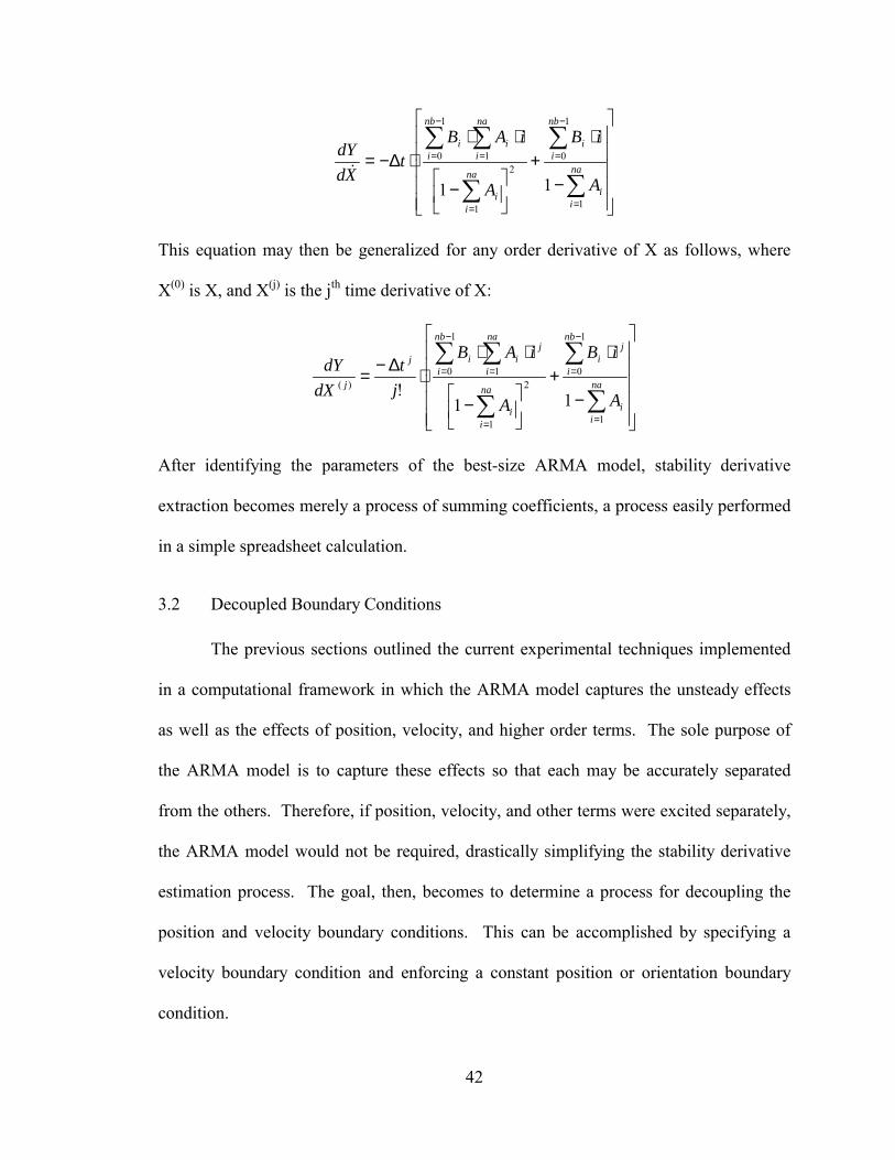
3.1.4 Extracting Stability Derivatives
Once the best ARMA model has been identified, extracting the steady and quasi-
steady stability derivatives from the ARMA model consists of applying steady and quasi-
steady conditions for the position and velocity terms and small perturbation theory for the
previous forces terms. This process is best described through a demonstration on a small
ARMA model with na equal to 2, nb equal to 3, and nr equal to 1. The ARMA model
The following is the MathCAD workspace used to calculate the Datcom estimates
for the stability derivatives including the available interference approximations. The
page numbers for the equations obtained from the Datcom are presented next to the
equation. The subscript w refers to the wing, v refers to the vertical tail, and h refers to
the horizontal tail.
115
Input parameters and initial calculations:
ARhbh
2
Sh:= ARv
bv2
Sv:=ARw
bw2
Sw:=
Clalpha .109180π
⋅:= Clalpha.MaClalpha
B:= 4.1.1.2-1 k
Clalpha.Ma B⋅
2 π⋅:= 4.1.3.2-3
qsweep w 0:= halfsweepw 0:= halfsweeph atan18
:= halfsweepv atan13
:=
CLalpha.wARw 2⋅ π⋅
2 ARwBk
⋅
21
tan halfsweepw( )( )2
B2+
⋅ 4++
:=
4.1.3.2-49
CLalpha.w 4.056=
CLalpha.hARh 2⋅ π⋅
2 ARhBk
⋅
21
tan halfsweeph( )( )2
B2+
⋅ 4++
:=
CLalpha.h 3.23=
Ma .4:= U0 13392Ma⋅:= roe 1.146 10 7−×:=
Sw 16:= Sv 6:= Sh 6:= cbarw 2:= Q .5 roe⋅ U02⋅:= B 1 Ma2−( ).5
:=
bw 8:= bh 4:= bv 3:= zv32
:=
lv 9.5:= lh 8.875:= lw .5:=
gama 5π
180⋅:= zw .5
bw2
sin gama( )2
⋅−:=
116
Longitudinal Stability Derivative Calculations:
Cmq 49.095−=
Cmq Cmq.w Cmq.h+:=Cmq.h 47.703−=
7.4.1.2-1Cmq.h 2−lh
cbarw
2
⋅ShSw
⋅ CLalpha.h⋅:=
Cmq.w 1.391−=
Cmq.w .7− Clalpha⋅cos qsweep w( )
B⋅
ARw .5lw
cbarw⋅ 2
lwcbarw
2
⋅+
⋅
ARw 2 cos qsweep w( )⋅+0+
18
+
⋅:=7.1.1.2-2
Cmalpha 4.304−=
Cmalpha Cmalpha.w Cmalpha.h+:=
Cmalpha.h 3.29−=
Cmalpha.hlh− CLalpha.h⋅
cbarw
Sh 1 down_wash−( )⋅
Sw⋅:=
4.5.2.1-2
4.4.1 7−down_wash .38785:=
Cmalpha.w 1.014−=
4.1.4.2-1Cmalpha.wlw− CLalpha.w⋅
cbarw:=
117
Yaw Moment Stability Derivative Calculations:
Cnr 2.745−=
Cnr Cnr.w Cnr.v+:=
Cnr.v 2.745−=
7.4.3.3-1Cnr.v 2lvbw
2
⋅ Cybeta.v⋅:=
at zero lift 7.1.3.3-2Cnr.w 0:=
Cnbeta 1.156=
Cnbeta Cnbeta.w Cnbeta.v+:=
Cnbeta.v 1.156=
5.6.3.1-1Cnbeta.v Cybeta.v−lvbw
⋅:=
5.3.1.1-3Cybeta.v CLalpha.v−Sv side_wash( )⋅
Sw⋅:=
5.4.1-1side_wash .724 3.06
SvSw
1 cos qsweep w( )+
⋅+ 0+ .009 ARw⋅+:=
CLalpha.vARv.eff 2⋅ π⋅
2 ARv.effBk
⋅
21
tan halfsweepv( )( )2
B2+
⋅ 4++
:=
ARv.eff 1.365=
5.3.1.1-2ARv.eff body intfer ARv⋅ 1 KH htailintfer 1−( )⋅+ ⋅:=
5.3.1.1-22KH .9:=htailintfer .9:=body intfer 1:=
at zero lift 5.1.3.1-1Cnbeta.w 0:=
118
Roll Moment Stability Derivative Calculations:
Clr 0.433=
Clr Clr.w Clr.v+:=
Clr.v 0.433=
7.4.3.2 1−Clr.v 2− lv⋅ zv⋅Cybeta.v
bw2
⋅:=
7.1.3.2 1−negligible at zero aoaClr.w 0:=
Clbeta 0.231−=
Clbeta Clbeta.w Clbeta.v+:=
Clbeta.v 0.183−=
at zero aoa 5.3.2.1 2−Clbeta.v Cybeta.vzvbw
⋅:=
Clbeta.w 0.049−=
5.1.2.1 2−at zero aoaClbeta.w gama dihedeff⋅1802
π2
⋅ compcor⋅:=
5.1.2.1 30a−compcor 1.14
+:=
5.1.2.1 29−dihedeff .00015−.00005
3−:=
VITA
Deric Austin Babcock
Candidate for the Degree of
Master of Science
Thesis: AIRCRAFT STABILITY DERIVATIVE ESTIMATION FROM FINITE ELEMENT ANALYSIS
Major Field: Aerospace Engineering
Biographical:
Personal Data: Born in Kingfisher, Oklahoma on July 21, 1980, the son of Larry R. Babcock and Sandra G. Babcock.
Education: Graduated from Lone Grove High School, Lone Grove Oklahoma, in
May 1998; received Bachelor of Science degree majoring in Mechanical and Aerospace Engineering from Oklahoma State University, Stillwater, Oklahoma, in May 2002; completed the requirements for the Master of Science degree in Mechanical Engineering at Oklahoma State University in July 2004.
Experience: Tutor, Mathematics Learning Resource Center, 1999-2001; Teaching
Assistant, OSU Mechanical and Aerospace Engineering Department, 2002-2004; Research Assistant, OSU MAE Dept. 2003-2004.
Professional Memberships: American Institute of Aeronautics and Astronautics,
American Society of Mechanical Engineers, Sigma Gamma Tau.