Stability,Bifurcation,andaPairofConservedQuantitiesina ...

Research ArticleStability Bifurcation and a Pair of Conserved Quantities in aSimple Epidemic System with Reinfection for the Spread ofDiseases Caused by Coronaviruses

Jorge Fernando Camacho 1 and Cruz Vargas-De-Leon 234

1Maestrıa en Ciencias de la Complejidad Universidad Autonoma de la Ciudad de Mexico Mexico City 03100 Mexico2Facultad de Matematicas Universidad Autonoma de Guerrero Av Lazaro Cardenas CU Chilpancingo 39087 GuerreroMexico3Seccion de Estudios de Posgrado e Investigacion Escuela Superior de Medicina Instituto Politecnico NacionalCiudad de Mexico Mexico4Division de Investigacion Hospital Juarez de Mexico Ciudad de Mexico Mexico

Correspondence should be addressed to Cruz Vargas-De-Leon leoncruz82yahoocommx

Received 24 July 2021 Accepted 3 November 2021 Published 26 November 2021

Academic Editor Hassan A El Morshedy

Copyright copy 2021 Jorge Fernando Camacho and Cruz Vargas-De-Leon is is an open access article distributed under theCreative CommonsAttribution License which permits unrestricted use distribution and reproduction in anymedium providedthe original work is properly cited

In this paper we study a modified SIRI model without vital dynamics based on a system of nonlinear ordinary differentialequations for epidemics that exhibit partial immunity after infection reinfection and disease-induced death is model can beapplied to study epidemics caused by SARS-CoV MERS-CoV and SARS-CoV-2 coronaviruses since there is the possibility thatin diseases caused by these pathogens individuals recovered from the infection have a decrease in their immunity and can bereinfected On the other hand it is known that in populations infected by these coronaviruses individuals with comorbidities orolder people have significant mortality rates or deaths induced by the disease By means of qualitative methods we prove that suchsystem has an endemic equilibrium and an infinite line of nonhyperbolic disease-free equilibria we determine the local and globalstability of these equilibria and we also show that it has no periodic orbits Furthermore we calculate the basic reproductivenumber (R0) and find that the system exhibits a forward bifurcation disease-free equilibria are stable when R0 lt 1σ and unstablewhen R0 gt 1σ while the endemic equilibrium consist of an asymptotically stable upper branch that appears from R0 gt 1σ σ beingthe rate that quantifies reinfection We also show that this system has two conserved quantities Additionally we show some of themost representative numerical solutions of this system

1 Introduction

Coronaviruses (CoVs) first discovered in a domestic poultryin the 1930s are a large family of viruses that can causerespiratory gastrointestinal liver and neurological diseasesin animals of all of them only seven coronaviruses areknown to cause disease in humans Four of these sevencoronaviruses most frequently cause symptoms of thecommon cold in rare cases they can produce severe lowerrespiratory tract infections including pneumonia mainly ininfants older people and the immunocompromised eother three of the seven led tomuchmore serious respiratory

illnesses in humans sometimes with fatal consequencesthan other coronaviruses and have caused major outbreaksof deadly pneumonia in this century SARS-CoV (also calledas SARS-CoV-1) identified as the cause of the severe acuterespiratory syndrome (SARS) MERS-CoV responsible forthe Middle East respiratory syndrome (MERS) and thenovel coronavirus SARS-CoV-2 identified as the cause ofcoronavirus disease 2019 (COVID-19) [1 2]

SARS-CoV was first detected in Guangdong Province ofChina in November 2002 and subsequently spread to morethan 30 countries [3] MERS-CoV was first identified inSeptember 2012 in Saudi Arabia although there is a

HindawiDiscrete Dynamics in Nature and SocietyVolume 2021 Article ID 1570463 18 pageshttpsdoiorg10115520211570463

documented outbreak in April 2012 in Jordan [4] and thenew strain of coronavirus SARS-CoV-2 was first reportedin the city ofWuhan China in late 2019 and since then it hasspread widely around the world becoming an ongoingpandemic [1] ese coronaviruses that cause severe respi-ratory infections in humans are zoonotic pathogens (theycan be transmitted from animals to people) Based on ex-tensive studies today it is known that SARS-CoV was ac-quired from civet and that contagions of MERS-CoV weretransferred by dromedary however the origin of the animaltransmission of SARS-CoV-2 has not yet been clarifiedRegarding SARS-CoV-2 it should be noted that it presents ahigh level of person-to-person contagion with respect to theother two Besides person-to-person spread not only occursthrough contact with infected secretions but also occurs viacontact with a surface contaminated by respiratory dropletsIt is known that symptomatic as well as asymptomatic andpresymptomatic patients can transmit the virus which bythe way appears more transmissible than SARS-CoV [1]

SARS-CoV MERS-CoV and by far currently SARS-CoV-2 have been responsible for serious epidemic respi-ratory infections with great international repercussion dueto their morbidity and mortality At the outbreak of SARS-CoV more than 8000 cases were reported worldwide with774 deaths whereas through 2019 worldwide nearly 2500cases of MERS-CoV infection (with at least 850 relateddeaths) have been reported from 27 countries [1] Howeveras for SARS-CoV-2 the numbers increased dramatically forjust over a year and it has spread to practically every countryin the world until July 21 of this year this pandemic hascaused 191148056 confirmed cases and 4109303 deaths[5] Since the great impact of the abovementioned data it isnot unnecessary to say that to overcome this global healthcrisis it is essential to study and understand the nature ofcoronaviruses their transmission characteristics spatialand temporal evolution preventive and therapeutic mea-sures and of course their complications

It should be mentioned that infection by SARS-CoV-2not only affects older people but also those with some type ofcomorbidity [6 7] as occurring in some countries of theAmerican continent such as Mexico [8] whose populationsshow high levels of overweight obesity diabetes and hy-pertension to name a few cases [9] e latent possibilitythat hospital services will collapse makes urgent the need foreffective medical treatments Instead of creating compoundsfrom zero that can take years to develop it has been chosento reuse drugs that are already approved for other diseasesand known to be safe Unapproved drugs that have workedwell in animal studies are also being tested with the other twofatal infections caused by SARS-CoV and MERS-CoV [10]Since there are currently no specific medications available toinhibit the viral replication of SARS-CoV-2 governmentmeasures each country has taken to limit its spread are basedon nonpharmaceutical interventions cancellation of massevents social distancing confinement measures and evencurfews [11] Although different types of SARS-CoV-2vaccines have been rapidly developed today and started to beapplied (to date only 26 of the worldrsquos population hasreceived at least one dose and 135 is fully vaccinated [12])

the impact of vaccination on the COVID-19 pandemic is farfrom significant since there are new outbreaks and it con-tinues to expand worldwide

Diseases caused by respiratory coronaviruses in humanshave the peculiarity of reinfecting them throughout theirlives [13] Although for example the persistence of anti-bodies against MERS-CoV has been found in infected in-dividuals almost three years after the outbreak of this diseasein Jordan in 2012 [14] for the case of SARS the duration ofimmunity has been estimated at more than 3 years [15] In acohort study 470 infected subjects with human coronavirus(HKU1 OC43 NL63 and 229E) were followed up for someyears In this cohort 85 of infected subjects had rein-fection with new or the same coronavirus occurring 155 and185 years respectively [16] A key unresolved question is theduration of acquired immunity in people recovered fromCOVID-19e recent appearance of SARS-CoV-2 preventsa direct study on this virus However there have been somestudies that suggest that recovered COVID-19 patients losetheir immunity within a few months [17 18] e first casesof two instances of SARS-CoV-2 infection in the same in-dividual have been reported in the United States [19] and inHong Kong [20] e first confirmed cases of reinfection inMexico were reported by Murillo-Zamora et al [11] Severalsystematic reviews have documented the different cases ofreinfection reported in the literature [21ndash23] To date nocohort studies have been reported on the follow-up of in-fected subjects who present reinfection with SARS-CoV-2[24]

Previous evidence indicates that a coronavirus reinfec-tion is likely is will be precisely one of our workinghypotheses in this research We will describe the temporalevolution of epidemics with these characteristics using acompartmental mathematical model based on a set ofnonlinear ordinary differential equations whose variablesare the different groups individuals or compartments of thecommunity affected by the infection according to their statewith respect to the disease [25 26] Mathematical modelsespecially compartmental ones play a fundamental role inunderstanding and predicting epidemics caused by thesedeadly coronaviruses such as the recent COVID-19 pan-demic Additionally they have also become one of the el-ements used by governments in the design of effective publicpolicies that allow satisfying the growing demand formedical attention that the population requires and theimplementation of social confinement measures to mitigateits growth

Since there is the possibility that individuals recoveredfrom these diseases present partial immunity and reinfec-tion we will use to describe them a SIRI (susceptible-in-fectious-recovered-infectious) model that takes bothcharacteristics into account in this model a population ofinfectious individuals can only recover temporarily and onceit recovers cannot remain that condition and become in-fected again [25]e SIRI model has already been applied tostudy these types of epidemics (with partial immunity andreinfection) from practical situations such as the effects ofvaccination based on the information available on a coro-navirus outbreak [27] to relevant analytical considerations

2 Discrete Dynamics in Nature and Society

of the model itself [28] is model has also been used todescribe epidemics of another type such as that caused byoverweight and obesity [29 30]

It has already been mentioned that SARS-CoV MERS-CoV and SARS-Cov-2 are viruses that cause epidemics withhigh death rates e description of this relevant aspect isalso part of the purposes of this research work One way toinclude this situation in our model is to expand it with anadditional variable which is the population of individualswho died due to the disease however this procedure has thegreat drawback since our system now has onemore variableof hindering its qualitative analysis An alternative way thatavoids the previous problem is to introduce a loss term thatwe identify as a disease-induced death term directly into theequation for the evolution of infected individuals the detailsof how this is proposed are given in the next section

Several transmission models have been developed for thedynamics of novel SARS-CoV infection [31ndash33] esemodels have considered the natural history of the disease aswell as the control measures such as quarantine and isola-tion but these have not considered the reinfectionphenomenon

In sum up in this work we propose a variant of the SIRImodel to describe epidemics in human populations causedby the previously described coronaviruses which have thepossibility of granting temporary immunity and reinfectionas well as causing high lethality e objective of this work isto analyze this system using the methods of the qualitativetheory of ordinary differential equations and show some ofthe most representative numerical solutions

e rest of this paper is organized as follows In Section2 we present our modified SIRI model and reduce it to atwo-dimensional system Section 3 focuses on qualitativeanalysis here we carry out a local analysis to establishequilibrium points and their corresponding local stabilitiesas well as bifurcations we also carry out a global analysisusing a suitable Lyapunov function to establish the globalstability of the endemic equilibrium and using the Dulaccriterion the absence of periodic orbits additionally weshow that our system presents two first integrals In Section4 some of the most representative numerical solutions ofour model are shown Finally in Section 5 we discuss theresults obtained and present our conclusions

2 Model

From a population or ldquomacroscopicrdquo point of view in theseepidemic outbreaks caused by the aforementioned coro-naviruses three types of populations of individuals can beidentified those infected I who by interacting with thesusceptible S get infected causing the eventual spread of thedisease throughout the population and recovered R whoapparently acquire immunity (cannot be infected again) anddo not affect the subsequent development of the epidemicOne of the most successful and common mathematical toolsthat describe the abovementioned situation is the epide-miological model SIR [34 35] In this S(t) I(t) and R(t)

denote the numbers of individuals in the groups or com-partments S I and R at time t respectively the total

population is considered to be of fixed size N so thatS(t) + I(t) + R(t) N In addition these epidemics havethe characteristic of developing rapidly that is they spreadin a relatively short time scale For this reason it is irrelevantto take into account in its description the natural births anddeaths of the population whose significant changes in sizeoccur over a much longer period In other words vitaldynamics factors or explicit demography can be neglected inour model [25 26]

Furthermore in our description of these types of epi-demic outbreaks we must take into account that individualsrecovered from the infection have temporary immunity andthe possibility of reinfection so considering a SIRI model (avariant of the SIR that incorporates these features) is moreconvenient [25 27 28] Since we will also consider that theseoutbreaks can present a high lethality with the purpose ofmodeling them we propose a modified SIRI model with adisease-induced death rate and without vital dynamicswritten in terms of the following set of ordinary differentialequations

dS

dt minus βSI

dI

dt βSI minus δI + σβRI minus αI

dR

dt δI minus σβRI

(1)

In equation (1) β δ α and σ are positive parameters thatrepresent the disease transmission recovery disease-in-duced death and recurrence rates respectively In thisdescription note that the value of parameter β depends onwhether the disease is more or less contagious 1δ is themean recovery period and σ is the reduction in suscepti-bility due to previous infection that takes values betweenzero and one (0lt σ lt 1) It should also be noted that system(1) is in effect a modified SIRI model the typical term σβRI

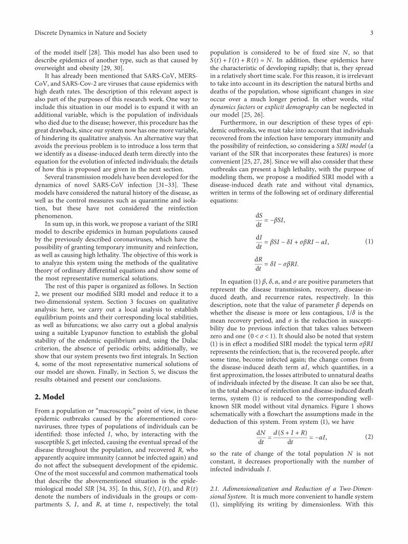
represents the reinfection that is the recovered people aftersome time become infected again the change comes fromthe disease-induced death term αI which quantifies in afirst approximation the losses attributed to unnatural deathsof individuals infected by the disease It can also be see thatin the total absence of reinfection and disease-induced deathterms system (1) is reduced to the corresponding well-known SIR model without vital dynamics Figure 1 showsschematically with a flowchart the assumptions made in thededuction of this system From system (1) we have

dN

dt

d(S + I + R)

dt minus αI (2)

so the rate of change of the total population N is notconstant it decreases proportionally with the number ofinfected individuals I

21 Adimensionalization and Reduction of a Two-Dimen-sional System It is much more convenient to handle system(1) simplifying its writing by dimensionless With this

Discrete Dynamics in Nature and Society 3

purpose we propose to change the variables of number ofindividuals S I R and the temporal t by the dimensionlessquantities [25]

x S

N

y I

N

z R

N

(3)

τ (δ + α)t (4)

e latter form is motivated by the fact that the pa-rameters α δ have dimensions of (units of time)minus 1 From (3)we have that N _x _S minus x _N N _y _I minus y _N and N _z _R minus z _Nnote that the point above the quantity in question indicatesits derivative with respect to time t On the other hand from(4) using the chain rule we obtain thatdxdt (δ + α)dxdτ dydt (δ + α)dydτ dzdt

(δ + α) dzdτ erefore system (1) written in terms ofthese new set of dimensionless variables takes the form

dx

dτ minus R0 minus ρ1( 1113857xy

dy

dτ minus y + R0xy + σR0yz + ρ1y

2

dz

dτ ρ2y minus σR0 minus ρ1( 1113857yz

(5)

where we have also defined the dimensionless quantities

ρ1 α

δ + α

ρ2 δ

δ + α

(6)

R0 βprime

δ + α (7)

which is called the basic reproductive number and thatrepresents the number of new infections produced by asingle infected person if the entire population is susceptibleR0 is commonly considered as a key parameter in the

evolution of the epidemic the smaller it is the slower theepidemic will be (in practice observing the epidemic makesit possible to measure R0 and consequently estimate βprime) In(7) we have defined the quantity βprime βN It should be notedthat since the parameters involved δ βprime are positive and α isnonnegative then 0le ρ1 lt 1 0lt ρ2 le 1 and 0ltR0 besideswe have that ρ1 + ρ2 1 Note that the new variables x y z

meet the condition

x + y + z 1 (8)

Taking into account precisely this condition it can beshown that the set of equations (5) can be simplified for thevariables y z in the two-dimensional system

dy

dτ R0 minus 1( 1113857y minus (1 minus σ)R0yz minus R0 minus ρ1( 1113857y

2

dz


(9)

It may be shown easily that the region of biological senseis

Λ (y z) isin R2|yge 0 zge 0 y + zlt 11113966 1113967 (10)

that is all solutions starting in Λ remain there for all τ ge 0Clearly the set Λ is positively invariant with respect tosystem (9)

22 Basic Reproductive Number e procedure in which R0was previously obtained is a consequence of rewritingsystem (1) by means of the dimensionless variables (3) and(4) in form (5) An alternative way of finding R0 is toconsider that initially S(0) S0 I(0)gt 0 with I(0)≪ S0 andR(0) 0 In this case second equation (1) takes the form

dI(0)

dt βS0 minus δ + σβR(0) minus α1113858 1113859I(0) (11)

Hence a necessary and sufficient condition for an initialincrease in the number of infected (since R(0) 0) isβS0 minus δ minus αgt 0 or equivalently R0 gt 1 where

R0 βS0

δ + αβprimex0

δ + α (12)

where x0 S0N On the other hand R0 lt 1 is the sufficientcondition to have an initial decrease of infected and that theepidemic does not spread us equation (12) is the ex-pression for R0 that we are looking for and is in completeagreement when x0 1 with equation (7) found previously

3 Analysis

31 Equilibria and Nullclines In order to find the equilib-rium points of system (9) we follow the usual way ofequating the left members of its equations with zero toobtain the values of the pair of variables (y z) that satisfythis equality As a result of this procedure we obtain twoequilibrium points One is disease-free equilibria of the form

S I

αI

σβIR

δI RβIS

Figure 1 Flowchart of the variant of model SIRI consideredis isthe well-known SIRmodel without vital dynamics with its term ofreinfection σβRI and modified by the term of disease-induceddeath αI


E0(0 z) (13)

with z isin R that is the straight line y 0 with an infinitenumber of points that constitute the vertical coordinate axisof the yz plane e second is the endemic equilibrium

Elowast

ylowast zlowast

( 1113857 σR0 minus 1σR0 minus ρ1

ρ2

σR0 minus ρ11113888 1113889 (14)

So the dynamics develop in region Λ and equilibriumpoints Elowast must be in the first quadrant of plane yz that isylowast ge 0 and zlowast gt 0 in other words σR0 minus ρ1 gt 0 andσR0 minus 1ge 0 Just when σR0 minus 1 0 Elowast is located on thevetical z-axis that is it is part of the points E0

An alternative way to find the equilibrium points of asystem is through the intersections of its nullclines [36 37]Since we will use these ideas later we will begin this dis-cussion below According to system (9) we have the null-clines dydτ 0 (vertical directions) given by the functions

z my + b y 0 (15)

which consist of two straight lines one of slope m minus (R0 minus

ρ1)[(1 minus σ)R0] and ordered to originb (R0 minus 1)[(1 minus σ)R0] and another that coincides with thevertical axis z In addition we have the nullclines dzdτ 0(horizontal directions) determined by

z zlowast

y 0(16)

which are again two lines one horizontal that cuts thevertical axis at point (0 ρ2(σR0 minus ρ1)) and another verticalthat also coincides with the z-axis It should be noted that as0lt σ lt 1 and R0 gt 0 the quantity (1 minus σ)R0 is always posi-tive consequently the slope of the vertical nullcline is onlydetermined by the sign of R0 minus ρ1 and its ordinate to theorigin by that of R0 minus 1 As we are interested in the points Elowast

located in region Λ it must happen thatσR0 minus ρ1 gt 0 σR0 minus 1ge 0 and σR0 minus ρ1 gt 0 as already men-tioned previously therefore note that R0 minus ρ1 (1 minus σ)R0 +

σR0 minus ρ1 gt 0 and R0 minus 1 (1 minus σ)R0 + σR0 minus 1gt 0ese lasttwo results imply that in region Λ the first vertical nullcline(15) must have a negative slope and its ordinate to the originpositive In addition it was also mentioned that for Elowast to bein Λ σR0 minus ρ1 gt 0 therefore the first horizontal nullcline(16) must be located in the upper half plane of plane yz

e intersections of different nullclines coincide with theequilibrium points Note that at y 0 nullclines overlap inboth vertical and horizontal directions therefore y 0consists of an infinite line of equilibrium points that is theequilibria E0 On the other hand another intersection be-tween the other different nullclines gives rise to point ElowastFigure 2 illustrates the nullclines (15) and (16) in a con-figuration compatible with region Λ it indicates horizontalnullclines in blue and verticals in red vertical axis z (ofinfinite equilibrium points) as well as equilibrium pointswith black circles is figure also shows the different di-rections that the vector field has along all the nullclines

e directions (left or right) of the horizontal nullclinesare determined by substituting z zlowast first equation (16) inthe first equation (9) which gives rise to

dy

dτ R0 minus ρ1( 1113857y y

lowastminus y( 1113857 (17)

To determine the positive or negative sign of (17) it isrequired to know the signs of ylowast (which depends in turn onthe signs of σR0 minus 1 and σR0 minus ρ1) the factor R0 minus ρ1 thevalues of y and their order relation with ylowast Since Λ issatisfied that σR0 minus ρ1 gt 0 σR0 minus 1ge 0 (that is ylowast ge 0) andR0 minus ρ1 gt 0(zlowast is on the nonnegative z-axis) the horizontalnullcline z zlowast cuts the nonnegative vertical axis at point(0 zlowast) and the nullcline of vertical directions first equation(15) at (ylowast zlowast) which is an equilibrium point ereforeaccording to (16) if ylowast ltyltinfin then dydτ lt 0 that is inthis interval the vector field is directed to the left if we are tothe right of (ylowast zlowast) when 0ltyltylowast then dydτ gt 0 so thatthe vector field points to the right if we are to the left of(ylowast zlowast) and to the right of (0 zlowast) while if minus infinltylt 0 thendydτ lt 0 that is the direction of the field is to the left if weare to the left of (0 zlowast) is result indicates that onhorizontal nullcline z zlowast the vector field leaves point(0 zlowast) and enters (ylowast zlowast)

e abovementioned analysis can be repeated for allcombinations of the quantities σR0 minus 1 σR0 minus ρ1 (whichdetermine the sign of ylowast ) and R0 minus ρ1 It can be shown thatthere are four possible cases For ylowast ge 0 if R0 minus ρ1 gt 0 thenvector field on the horizontal nullcline z zlowast leaves (0 zlowast)

and enters (ylowast zlowast) and when R0 minus ρ1 lt 0 it enters (0 zlowast)

and leaves (ylowast zlowast) Figure 2(a) illustrates the first case Alsofor ylowast lt 0 if R0 minus ρ1 gt 0 then field enters (0 zlowast) and leaves(ylowast zlowast) and when R0 minus ρ1 lt 0 it leaves (0 zlowast) and enters(ylowast zlowast) Figure 2(b) shows the third case Note that only inthe first case the equilibrium points are in region Λ

On the other hand the directions (up or down) of thevertical nullclines are determined by replacing the verticalnullcline first equation (15) in the second equation (9)which allows obtaining

dz

dτ minus

R0 minus ρ1( 1113857 σR0 minus ρ1( 1113857

(1 minus σ)R0y ylowast

minus y( 1113857 (18)

In order to determine the positive or negative sign of(18) we need to know the signs of ylowast (that depends on thesigns of σR0 minus 1 and σR0 minus ρ1) the factor R0 minus ρ1 the valuesof y and their relation with ylowast Since in Λ we have thatσR0 minus ρ1 gt 0 σR0 minus 1ge 0 R0 minus ρ1 gt 0 and R0 minus 1gt 0 the firstvertical nullcline (16) cuts horizontal nullcline z zlowast at theequilibrium point (ylowast zlowast) and the positive vertical axis atthe point (0 b) and has a negative slope ereforeaccording to (18) if ylowast ltyltinfin then dzdτ gt 0 that is inthis interval the direction of the vector field is up while if0ltyltylowast then dzdτ lt 0 so that in this interval directionsare down and when minus infinltylt 0 dzdτ gt 0 in this intervaldirections are up

A complete analysis of the directions (up or down) ofthis vertical nullcline requires taking into account allcombinations of signs of the quantities σR0 minus 1 σR0 minus ρ1 and


R0 minus ρ1 It can also be shown that there are four possiblecases For ylowast gt 0 if R0 minus ρ1 and σR0 minus ρ1 are of oppositesigns then the direction of vector field on this verticalnullcline is down in the interval minus infinltylt 0 is up in0ltyltylowast and is down in ylowast ltyltinfin whereas if R0 minus ρ1 andσR0 minus ρ1 are of the same signs then the vector field is up inminus infinltylt 0 down in 0ltyltylowast and up in ylowast ltyltinfinFigure 2(a) illustrates the second case Besides for ylowast lt 0 ifR0 minus ρ1 and σR0 minus ρ1 are of opposite signs then the vectorfield is down in minus infinltyltylowast up in ylowast ltylt 0 and down in0ltyltinfin whereas if R0 minus ρ1 and σR0 minus ρ1 are of the samesigns then the vector field is up in minus infinltyltylowast down inylowast ltylt 0 and up in 0ltyltinfin Figure 2(b) shows the fourthcase Note that only in the second case the equilibriumpoints are in region Λ

32 Local Stability In order to determine the stability ofthese families of equilibrium points we need to calculate theJacobian matrix of system (9) and evaluate it on them ismatrix overall is given as

J(y z) minus (1 minus σ)R0z minus 2 R0 minus ρ1( 1113857y + R0 minus 1 minus (1 minus σ)R0y

ρ2 minus σR0 minus ρ1( 1113857z minus σR0 minus ρ1( 1113857y1113888 1113889

(19)

To perform the local stability analysis we will considerseparately the disease-free equilibria and the endemicequilibrium cases

321 e Disease-Free Equilibria E0 (0 z) e Jacobianmatrix (19) evaluated in the disease-free equilibria E0 takesthe simple form

J(0 z) minus (1 minus σ)R0z + R0 minus 1 0

ρ2 minus σR0 minus ρ1( 1113857z 01113888 1113889 (20)

whose eigenvalues are λ1 0 and λ2 minus (1 minus σ)R0z + R0 minus 1Note that these equilibrium points are nonhyperbolic Dueto this nature of the points E0 and the infinite number ofthem it is quite difficult to determine their stability One wayto visualize the dynamics around them is through a geo-metric analysis of the nullclines of system (9) is allows usto find the directions left or right of the vector field along thehorizontal nullclines and its directions up or down on thevertical nullclines in particular this gives a glimpse of how itis around the equilibrium points Of particular interest hereare the results of the analysis performed in the previoussection of the directions of the vector field on the horizontalnullclines z zlowast around their point of intersection (0 zlowast)

with the vertical axis z ose results rewritten in terms ofthe ideas of stability can be written in the following way forylowast gt 0 if R0 minus ρ1 gt 0 then point (0 zlowast) is unstable and whenR0 minus ρ1 lt 0 it is stable whereas for ylowast lt 0 if R0 minus ρ1 gt 0 thenpoint (0 zlowast) is stable and whenR0 minus ρ1 lt 0 it is unstable seeFigure 2 Since we have an infinite number of points alongthe vertical axis z the stability along a horizontal line thatcuts one of them say (0 zlowast) must be identical to the stabilityfound at its intersection with the horizontal nullcline z zlowastIt should be noted that the analysis based on the method ofthe nullclines reveals that points (0 zlowast) are stable if zgt b andunstable if zlt b see again Figure 2

Since 0lt σ lt 1 and 0le ρ1 lt 1 we can establish the re-lations 0le ρ1 lt ρ1σ and ρ1σ lt 1σ besides that we knowthat 1lt 1σ therefore the order relation between thesequantities is 0le ρ1 lt ρ1σ lt 1σ ltinfin which will be calledsegment L On the other hand it has just been mentionedthat the stability of the nonhyperbolic points (0 zlowast) dependson the signs of σR0 minus ρ1 σR0 minus 1 and R0 minus ρ1 or in otherwords it depends of the location that R0 has in L

us when σR0 minus ρ1 gt 0 σR0 minus 1ge 0 (which determinethat ylowast gt 0) and R0 minus ρ1 gt 0 according to segment L theintersection of these three subintervals is 1σ ltR0 ltinfin Since

Z

y

E(yz)E0(0z)

y

b

0

(a)

E(yz) E0(0z)

y y

Z

b

0

(b)

Figure 2 Representation of nullclines of system (9) horizontal direction z zlowast (in blue) and vertical direction z my + b (in red) thevertical axis z(y 0) is a combination of both Equilibrium points are indicated by black circles (a) σR0 minus ρ1 gt 0 σR0 minus 1gt 0 R0 minus ρ1 gt 0and R0 minus 1gt 0 (b) σR0 minus ρ1 gt 0 σR0 minus 1lt 0 R0 minus ρ1 gt 0 and R0 minus 1gt 0


the previous stability result establishes that in this situationpoints (0 zlowast) are unstable we conclude that the equilibriumpoints E0 are unstable when 1σ ltR0 ltinfin On other handwhen σR0 minus ρ1 gt 0 σR0 minus 1lt 0 and R0 minus ρ1 gt 0 according toL intersection is ρ1σ ltR0 lt 1σ since points (0 zlowast) arestable here we have that points E0 are unstable whenρ1σ ltR0 lt 1σ By means of an analysis similar to theprevious one it can be shown that points E0 are unstable inρ1 ltR0 le ρ1σ and stable in 0leR0 lt ρ1 ese obtained re-sults can be summarized as follows

Theorem 1 Disease-free equilibrium points E0 whichconstitute the vertical axis z are nonhyperbolic ese pointsare

(i) unstable if 1σ ltR0 ltinfin and ρ1 ltR0 lt ρ1σ(ii) stable if ρ1σ ltR0 lt 1σ and 0ltR0 lt ρ1

Since when α 0 our model is reduced to the con-ventional SIRI model in this situation ρ1 0 so fromeorem 1 it follows that the nonhyperbolic equilibriumpoints E0 are stable if 0ltR0 lt 1σ and unstable if1σ ltR0 ltinfin

322 e Endemic Equilibrium Elowast (ylowast zlowast) Bysubstituting the endemic equilibrium Elowast (ylowast zlowast) in sys-tem (9) the identities are obtained

minus (1 minus σ)R0zlowast

R0 minus ρ1( 1113857ylowast

minus R0 minus 1( 1113857

ρ2 minus σR0 minus ρ1( 1113857zlowast

0(21)

which allows writing the Jacobian matrix (19) evaluated insuch a point as

J ylowast zlowast

( 1113857 minus R0 minus ρ1( 1113857y

lowastminus (1 minus σ)R0y

lowast

0 minus σR0 minus ρ1( 1113857ylowast1113888 1113889 (22)

e trace of (22) is given by

Tr J 2ρ1 minus (σ + 1)R01113858 1113859ylowast

2ρ1 minus (σ + 1)R01113858 1113859 σR0 minus 1( 1113857

σR0 minus ρ1

(23)

and its determinant is

Det J R0 minus ρ1( 1113857 σR0 minus ρ1( 1113857ylowast2

R0 minus ρ1( 1113857 σR0 minus 1( 1113857

2

σR0 minus ρ1

(24)

whereas it can be shown that its discriminant defined asΔ Tr J2 minus 4Det J is

Δ minus (1 minus σ)R0ylowast

1113858 11138592

(1 minus σ)

2R20 σR0 minus 1( 1113857

2

σR0 minus ρ1( 11138572 (25)

which is a nonnegative quantity According to the trace-determinant plane method [36ndash38] the analysis of matrix(22) indicates that points Elowast since Δge 0 can be saddlepoints (if Det Jlt 0) and degenerate equilibrium (ifDet J 0) or nodes of two ldquostraight-linerdquo solutions (if

Det Jgt 0) the latter pair being stable or unstable if Tr Jlt 0 orTr Jgt 0 respectively Furthermore the eigenvalues of (22)are given by

λ12 12

(Tr J plusmnΔ

radic) (26)

which can be explicitly written as

λ1 minus R0 minus ρ1( 1113857ylowast

minusR0 minus ρ1( 1113857 σR0 minus 1( 1113857

σR0 minus ρ1 (27)

λ2 minus σR0 minus ρ1( 1113857ylowast

minus σR0 minus 1( 1113857 (28)

Note that eigenvalues (27) and (28) are functions of R0and their signs will depend on the location of this quantity insegment L already indicated above In general they aredifferent from zero so the equilibrium points Elowast arehyperbolic

Next we will analyze the signs that λ1 and λ2 could havein L According to (27) and (28) λ1 lt 0 and λ2 lt 0 ifσR0 minus 1gt 0 R0 minus ρ1 gt 0 and σR0 minus ρ1 gt 0 the intersection ofthese three subintervals occurs at 1σ ltR0 ltinfin so in thisregion the equilibrium points Elowast correspond to nodes oftwo ldquostraight-linerdquo solutions that are locally asymptoticallystable In this case in which both eigenvalues are negativepoints Elowast lie within region Λ however for other combi-nations of signs of the eigenvalues λ1 and λ2 points Elowast lieoutside of Λ us it can be shown that λ1 gt 0 and λ2 gt 0when ρ1σ ltR0 lt 1σ and 0leR0 lt ρ1 so that in these regionspoints Elowast correspond to unstable nodes of two ldquostraightlinesrdquo Additionally λ1 gt 0 and λ2 lt 0 if ρ1 ltR0 lt ρ1σ sothere points Elowast are saddle points the case λ1 lt 0 and λ2 gt 0does not exist because the intersection of the correspondingsubintervals gives rise to the empty set Moreover λ1 0 andλ2 gt 0 when R0 ρ1 so here Elowast is a singly degenerateequilibrium Lastly λ1 λ2 0 when R0 1σ so Elowast is adoubly degenerate equilibrium ese last two cases corre-spond to nonhyperbolic equilibrium points e previousresults are summarized in eorem 2

Theorem 2 e endemic equilibrium points Elowast are ingeneral hyperbolic Such points are

(i) nodes (of two ldquostraight-linerdquo solutions) locally as-ymptotically stable if 1σ ltR0 ltinfin

(ii) a doubly degenerate equilibrium if R0 1σ (inwhich case it is nonhyperbolic)

(iii) unstable nodes (of two ldquostraight-linerdquo solutions) if0leR0 lt ρ1 and ρ1σ ltR0 lt 1σ

(iv) saddle points if ρ1 ltR0 lt ρ1σ(v) a singly degenerate equilibrium if R0 ρ1 (in which

case it is nonhyperbolic)(vi) unstable nodes (of two ldquostraight-linerdquo solutions) if

0leR0 lt ρ1

It is important to note that in eorem 2 subinterval1σ ltR0 ltinfin (that of condition i)) is the only one thatguarantees that points Elowast are in region Λ Again since when


α 0 our model is reduced to the conventional SIRI modelin this situation ρ1 0 so for this case from eorem 2 itfollows that the equilibrium points Elowast are nodes (of twoldquostraight-linerdquo solutions) locally asymptotically stable if1σ ltR0 ltinfin and unstable if 0ltR0 lt 1σ

33 Presence of a Forward Bifurcation e analysis thatallowed to formulate the two previous theorems shows thatthe coordinates of both points E0 and Elowast are a function ofthe reproductive number R0 In particular it is of greatinterest to know how the family of equilibrium points ylowast

(which is the abscissa of points Elowast) varies with R0 and tovisualize such dependence in a diagram R0y

lowast this is im-portant because R0 could play the role of a bifurcationparameter For our study problem the ylowast families consist oftwo curves one horizontal line ylowast 0 of disease-freeequilibrium points located on the R0 axis and another de-termined by

ylowast

R0( 1113857 σR0 minus 1σR0 minus ρ1

(29)

of endemic equilibrium points By inspection it can be seenthat equation (29) has a discontinuity at R0 ρ1σ whichgives rise to one left branch that cuts the vertical axis at ylowast

1ρ1 when R0 0 and moves upward indefinitely as R0approaches to R0 ρ1σ as well as another right branch forvalues greater than R0 ρ1σ that comes from below cuttingto the horizontal axis at R0 1σ and asymptotically ap-proaches to the horizontal line ylowast 1 as R0 tends to infinitysee Figure 3

Figure 3 in fact is the schematic representation of theresults of the two previous theorems both illustrate thebehavior of the different families of equilibrium points as afunction of R0 according to their positions in segment L

defined above us for example this figure shows howthese families exhibit an abrupt change at the point (0 1σ)in other words in this nonhyperbolic point a bifurcationoccurs Besides it also indicates in gray the region of bi-ological sense Λ is bifurcation diagram corresponds towhat is called as forward bifurcation [26] It should be notedthat this type of bifurcation is really a kind of transcriticalbifurcation [37 38] with bifurcation point (0 1σ) that is itconsists of a horizontal branch that coincides with the R0axis which is stable before the bifurcation point and un-stable after it and another branch that is unstable below thebifurcation point and stable above it see again Figure 3

34 Nonexistence of Periodic Orbits and Global StabilityWe will now discuss two results directly related to the globalbehavior of the trajectories of system (9) ese are thenonexistence of periodic orbits in the region of biologicalsense Λ and the global stability of the endemic equilibriumpoint Elowast in the said region

341 Nonexistence of Periodic Orbits e nonexistence ofperiodic orbits in the two-dimensional system (9) implies of

course that neither system (5) has this type of trajectoriese first statement is shown in eorem 3

Theorem 3 System (9) does not have periodic orbits in theinterior of Λ

Proof Let us identify the right-hand parts of the system ofequations (9) as

P(y z) equiv R0 minus 1( 1113857y minus (1 minus σ)R0yz minus R0 minus ρ1( 1113857y2

Q(y z) equiv ρ2y minus σR0 minus ρ1( 1113857yz(30)

We propose the Dulac function

Φ(y z) 1y

(31)

In this way it can be easily verified that

z(ΦP)

zy+

z(ΦQ)

zz minus σR0 minus ρ1( 1113857 + R0 minus ρ1( 11138571113858 1113859lt 0 (32)

since as mentioned in Section 3 in Λ it is true that σR0 minus

ρ1 gt 0 and as a consequence in this region R0 minus ρ1 gt 0erefore according to the Dulac criterion [37 38] there areno periodic orbits in the interior of Λ

342 Global Stability of the Endemic Equilibrium PointWe will establish the conditions that the endemic equilib-rium point Elowast must meet to guarantee its global stabilityis will be carried out by following Lyapunovrsquos secondmethod or Lyapunov stability theorem [37 38] as is shownin eorem 4

Theorem 4 e unique endemic equilibrium Elowast is globallyasymptotically stable in the interior of Λ

Proof We consider the common quadratic Lyapunovfunction

y

1ρ1

R0ρ1σ 1σρ1

1

0

Λ

Figure 3 Bifurcation diagram of system (9) Locally asymptoticallystable and unstable points have been indicated respectively withcontinuous and discontinuous lines e region of biological senseΛ is indicated with gray color


V(y z) 12

y minus ylowast

( 11138572

+R0(1 minus σ)

2 σR0 minus ρ1( 1113857z minus zlowast

( 11138572 (33)

which is continuous and a positive definite functionV(y z)gt 0 in a region that contains Elowast (ylowast zlowast) that is inturn located in Λ It can be verified by inspection thatV(y z) takes the value V(y z) 0 at Elowast so that the globalminimum value of V(y z) is located at that point Calcu-lating the total derivative of (32) and using the two-di-mensional system (9) we obtain

ddτ

V(y z) zV

zy

dy

dτ+

zV

zz

dz

dτ

y minus ylowast

( 1113857 R0 minus 1( 1113857y minus (1 minus σ)R0yz minus R0 minus ρ1( 1113857y2

1113960 1113961

+R0(1 minus σ)

σR0 minus ρ1z minus zlowast

( 1113857 ρ2y minus σR0 minus ρ1( 1113857yz1113858 1113859

(34)

Taking into account the relations (21) the previousexpression (34) takes the form

ddτ

V(y z) minus y14

(3 + σ)R0 minus ρ11113876 1113877 y minus ylowast

( 11138572

minus y(1 minus σ)R012

y minus ylowast

( 1113857 + z minus zlowast

( 11138571113876 11138772lt 0

(35)

Note in (35) that (14)(3 + σ)R0 minus ρ1

R0 minus ρ1 minus (14)(1 minus σ)R0 gt 0 in regionΛ this is true since asalready mentioned R0 minus ρ1 (1 minus σ)R0 + σR0 minus ρ1 gt 0 insuch a region so that R0 minus ρ1 gt (1 minus σ)R0 and as

(1 minus σ)R0 gt (14)(1 minus σ)R0 we finally obtainR0 minus ρ1 minus (14)(1 minus σ)R0 gt 0us since also (1 minus σ)R0 gt 0the negative inequality in (35) holds for all ygt 0 andzgt 0 that is for every point Elowast located in Λ (except thepositive coordinate axes and the origin) ereforeaccording to Lyapunov stability theorem the endemicequilibrium Elowast is globally asymptotically stable in theinterior of Λ

35 Existence of Two First Integrals In this section we willrefer to the three-dimensional system (5) instead of the two-dimensional one (9) It was found that system (5) has aninteresting characteristic it has two quantities that are in-variant in time along their trajectories that is it has two firstintegrals

To show this first note that starting with (2) and using(3) (4) and (8) we obtain

d(x + y + z)

dτ 0 (36)

so that (8) is in itself worth the redundancy a relation amongthe variables x y and z that remains constant ereforethis is a first integral as shown below

Theorem 5 Dynamic system (5) has a first integral given by

H1(x y z) x + y + z (37)

Proof Calculating the total derivative of (37) and using thethree equations (5) we have

ddτ

H1(x y z) zH1

zx

dx

dτ+

zH1

zy

dy

dτ+

zH1

zz

dz

dτ

minus R0 minus ρ1( 1113857xy minus y + R0xy + σR0yz + ρ1y2

+ ρ2y minus σR0 minus ρ1( 1113857yz

y ρ2 + ρ1(x + y + z) minus 11113858 1113859

y ρ1 + ρ2 minus 1( 1113857 0

(38)

since (8) is true and also ρ1 + ρ2 1 e proof iscomplete

On the other hand note that the first and third equations(5) are only coupled by the variable y therefore by formingthe quotient between them we obtain

dx

dz minus

R0 minus ρ1( 1113857x

ρ2 minus σR0 minus ρ1( 1113857z (39)

is expression can be solved in principle by themethod of separating variables giving rise to

1R0 minus ρ1

ln x 1

σR0 minus ρ1ln ρ2 minus σR0 minus ρ1( 1113857z1113858 1113859 + C (40)

where C is a integration constant It can be shown that aftersome algebraic steps it gives rise to

ρ2σR0 minus ρ1

minus z1113888 1113889xminus σR0minus ρ1( )R0minus ρ1( ) K (41)

K being a constant quantity Consequently we have ob-tained a quantity dependent on the variables x and z whichremains constant for all τ It turns out that this quantity isalso a first integral as shown below


Theorem 6 Dynamic system (5) has another first integralgiven by

H2(x z) ρ2

σR0 minus ρ1minus z1113888 1113889x

minus σR0minus ρ1( ) R0minus ρ1( )( ) (42)

Proof Calculating the total derivative of (39) and using thefirst and third equations (5) we have

ddτ

H2(x z) zH2

zx

dx

dτ+

zH2

zz

dz

dτ

σR0 minus ρ1R0 minus ρ1

1113888 1113889ρ2


minus σR0minus ρ1( )R0minus ρ1( )minus 1R0 minus ρ1( 1113857xy

minus xminus σR0minus ρ1( )R0minus ρ1( ) ρ2y minus σR0 minus ρ1( 1113857yz1113858 1113859

ρ2yxminus σR0minus ρ1( )R0minus ρ1( ) minus σR0 minus ρ1( 1113857yzx

minus σR0minus ρ1( )R0minus ρ1( )

minus ρ2yxminus σR0minus ρ1( )R0minus ρ1( ) + σR0 minus ρ1( 1113857yzx

minus σR0minus ρ1( )R0minus ρ1( ) 0

(43)

e proof is complete

It should be noted that expression (42) is reduced whenα 0 to the first integral of Lemma 1 reported in [28] Inthis sense the former is a generalization of the latter

351 Calculation of the Maximum of y(τ) e calculationof the first previous integrals allows us to estimate forexample without having to know the corresponding exactsolution the maximum value that the infectious proportiony(τ) reaches To do this we first consider that we have theinitial conditions x(0) x0 and z(0) z0 us it can beshown that from (41) we obtain

z ρ2

σR0 minus ρ1minus

ρ2σR0 minus ρ1

minus z01113888 1113889x

x01113888 1113889

σR0minus ρ1( )R0minus ρ1( )

(44)

erefore using (8) and (44) we have the followingexpression for the variable y written only in terms of x

y 1 minus x minusρ2

σR0 minus ρ1+

ρ2σR0 minus ρ1

minus z01113888 1113889x

x01113888 1113889


(45)

Equating the derivative of y(τ) with respect to τ to zeroallows us to find its critical point by deriving (45) in thisway it can be shown that this point is given by

1113954x x0R0 minus ρ1( 1113857x0

ρ2 minus z0 σR0 minus ρ1( 11138571113890 1113891

minus R0minus ρ1( )(1minus σ)R0( )(46)

and also that it is a maximumerefore substitution of (46)in (45) allows us to find the maximum of the infectiousproportion y(τ) at any value of τ and in the presence of theparameter α which we will denote as ymaxα that is

ymaxα 1 minusρ2

σR0 minus ρ1+

R0 minus ρ1σR0 minus ρ1

minus 11113888 1113889ρ2 R0 minus ρ1( 1113857( 1113857 minus z0 σR0 minus ρ1( 1113857 R0 minus ρ1( 1113857( 1113857

xσR0minus ρ1( )R0minus ρ1( )

0

⎡⎢⎢⎢⎢⎣ ⎤⎥⎥⎥⎥⎦

R0minus ρ1(1minus σ)R0( )

(47)

It should be noted that equation (47) reduces completelywhen the limit case α⟶ 0 is taken (that is ρ1⟶ 0 andρ2⟶ 1) to expression (ii) (a) of eorem 1 in [28] In thissense our expression represents a generalization of that onefor the case in which the parameter α of disease-induceddeath is taken into account

On the other hand by means of equation (47) an estimatecan bemade of the difference between themaximumvalues ofy

in the presence and absence of the parameter α that isymaxα minus ymaxα0 If we consider α small (α≪ 1) we can ap-proximate definitions (6) by ρ1≃αδ and ρ2≃1 erefore forthis situation it can be shown that the said difference is given by


ymaxα minus ymaxα0 ≃1σ

minus 1 minusα

δσR01113888 1113889

1R0( 1113857 minus z0σ + z0αδR0( 1113857

xσminus αδR0( )0

⎡⎢⎢⎢⎢⎣ ⎤⎥⎥⎥⎥⎦

(1(1minus σ))minus αδ(1minus σ)R0( )

minus1σ

minus 11113874 11138751R0( 1113857 minus z0σ

xσ0

1113888 1113889

(1(1minus σ))

(48)

A slight simplification of expressions (47) and (48) canbe obtained if we consider z0 0 in them that is there areno infected individuals at the beginning of the epidemic

4 Numerical Results

In this section we will present some of the most repre-sentative numerical solutions of our model that allow us toillustrate the different results obtained previously eparameter values that we will use to calculate them cor-respond to estimates made for the epidemic caused bySARS-CoV-2 To carry out the numerical analysis it isnecessary to know representative values of the parametersinvolved in our model namely the βprime δ α and σ ratesRegarding this disease COVID-19 patients in Wuhanshowed that the average contagious period of SARS-CoV-2was 20 days [39] We choose a value of 14 days to thecontagious period (1δ) of an infected person so thatδ≃0071 dayminus 1 Furthermore the disease-induced deathrate has been reported inMexico of 00127 and 00259 dayminus 1

[40] although more studies are lacking where disease-induced death rate is estimated in populations with a highprevalence of comorbidities or in old populations We willconsider that α≃01 however in our calculations we willvary this rate and consider that 0le αlt 1 It is worthmentioning that such a percentage depends on the par-ticular characteristics of the population of each country andmay be a little higher as in the case of Mexico [8] if itpresents several comorbidities [6 7] A meta-analysis [41]of the basic reproductive number (R0) to China reported apooled estimation of 332 (95 confidence interval281 382) Knowing this quantity is important becausefrom it the approximate values of the other two remainingrates that are relevant in our model can be obtained Wetake a value of R0≃311 (as in [42]) us according to theparameters indicated from relation (7) it follows thatβprime≃0532 dayminus 1 Finally it has already been mentioned thatthe bifurcation occurs when R0 1σ so a first estimate ofthe relapse rate although it is for this case is σ≃0322precisely in this model 0lt σ lt 1 and in our calculationsthis quantity will vary taking values belonging to this in-terval e magnitudes of the indicated rates δ α βprime and σare shown in Table 1

Since the purpose here is to show the effects produced inthe population of infected individuals y(τ) basically by thechange of the α and σ rates we will take the quantitiesindicated in Table 1 only as a reference that is in the dif-ferent cases that we will present below we will make some ofthem take values close to or different (even by several ordersof magnitude) from those reported there

41 Effects on the Trajectories ofy(τ) due toVariations of the αand σ Rates We illustrate how changing the rates α and σaffects the dynamics of the solutions of system (9) inparticular those of the proportion of infected individualsy(τ) For the different cases to be considered we will in-dicate the values of R0 (since it varies inversely with α as ispointed out by (7)) and their corresponding bifurcations 1σAlso for each of the graphs obtained taking into account(47) we will indicate the magnitude that reaches its peaknamely ymaxα

Let us consider a first case where α varies βprime 0532δ 0071 (as in Table 1) and σ 01 will be fixed We havechosen this last magnitude for the recovery rate so that R0remains below the value of the bifurcation 1σ 10 that isconstant Figure 4 shows how the graphs of y(τ) change forthree different values of α specifically for α 00001 (blueline) R0 748 and ymaxα 063 when α 01 (red line)R0 311 and ymaxα 051 and for α 017 (green line)R0 221 and ymaxα 041 In this figure it can be seen thatas α grows the peak of the graphs decreases they widen andshift to the right and they are also less biased Note that inthe first case (α 00001) the rate α is so small that the effectproduced is as if it were not there in the absence of α(α 0)R0 (for fixed βprime and δ) has its greatest value and the graph ofy has its highest peak Apparently the inclusion in themodelof the rate α produces a more adequate description of theevolution of infected individuals since its absence causesoverestimated values of R0 and the peak of its graph

Now we consider a second case where σ changesβprime 0532 δ 0071 (as in Table 1) and α 01 will befixed Note that in this situation for each σ we will havedifferent bifurcation values 1σ so that if σ is very close tozero the bifurcation point is much greater than one whereasif it is very close to one this point is much less than one Wechoose the magnitudes of σ that allow to R0 311 (whichdoes not change since βprime δ and α are constant) to be belowor above the value of the bifurcation Figure 5 illustrates howthe temporal evolution of y(τ) changes for three differentmagnitudes of σ particularly when σ 01 (blue line) 1σ

10 and ymaxα 051 when σ 03 (red line) 1σ 333 andymaxα 058 and for σ 04 (green line) 1σ 25 andymaxα 062is figure shows how as σ grows the graphs ofy(τ) change their peaks increase widen and shift slightly tothe right It should be noted that when σ 01 (blue line)and σ 03 (red line) R0 is below their corresponding bi-furcation values and both trajectories tend to a disease-freeequilibrium point E0 as τ tends to infinity while when σ

04 (green line) R0 is above its bifurcation value and thetrajectory tends to an endemic equilibrium point Elowast as τtends to infinity


Finally let us consider a third case which certainlycould be considered as a combination of the previous twoHere α varies βprime 0532 and δ 0071 (as in Table 1) butnow σ 017 will be a different fixed value We haveconsidered this latter magnitude in order that R0 as α in-creases may exceed the value of the bifurcation 1σ 588that does not change e different rates α selected make R0take values below or above the bifurcation 1σe effect thatthis has on the y curves is illustrated in Figure 6 us in thefigure when α 00001 (blue line) R0 748 andymaxα 065 the curve is above the value of the bifurcationand tends to an endemic equilibrium point as time tends toinfinity If α 01 (red line) R0 311 and ymaxα 053whereas when α 017 (green line) R0 221 andymaxα 043 in both cases R0 is below the value of thebifurcation so the curves tend to disease-free equilibriumpoints as time tends to infinity Note that variations in the

rate α can produce changes in the nature of the equilibriumpoints towards which the y curves tend as α increases thecurves go from tending towards an endemic equilibriumpoint Elowast (when α 00001) to others free of disease E0 (ifα 01 or α 017)

42 Phase Portraits before and during Forward BifurcationWe present here some representative phase portraits ofdynamic system (9) for different values of R0 between 0 andjust over 1σ the bifurcation value taking as reference thediagram in Figure 3 Figures 7ndash12 illustrate the differentphase portraits that were calculated For the realization ofthese graphs the rates δ α and σ were considered asconstants the first with its value given in Table 1 and theother two with magnitudes equal to 01 and 017 respec-tively the rate βprime was varied e quantity R0 can increase its

Table 1 Estimation of the values of the main parameters used in the model which correspond to the SARS-CoV-2 coronavirus

Parameter Meaning (unit) Estimated valuesβprime Transmission rate(dayminus 1) 0532δ Recovery rate(dayminus 1) 0071σ Relative susceptibility of recovered individuals (adimensional) Varyingα Disease minus induced death rate(dayminus 1) Varying

50 10 15 20 25 30τ

07

06

05

04

03

02

01

y

Figure 4 Evolution of y(τ) for the fixed parameters βprime 0532 δ 0071 and σ 01 α 00001 blue line α 01 red line and α 017green line

50 10 15 20 25 30τ

07

06

05

04

03

02

01

y

Figure 5 Evolution of y(τ) for the fixed parameters βprime 0532 δ 0071 and α 01 σ 01 blue line σ 03 red line and σ 04 greenline


value according to (7) if δ is kept constant and α decreasesor βprime increases It has been pointed out that the absence ofthe parameter α causes an overestimated magnitude of R0 sowe will keep its value fixed and we will only vary βprime in anincreasing way For rates δ α and σ already mentioned inaccordance with (6) we have that ρ1≃05848 ρ2≃04152while ρ1σ≃3440 and 1σ≃5882 For each value of R0 wewill also indicate the values of their corresponding disease-free E0 (0 z) and endemic Elowast (ylowast zlowast) equilibriumpoints expressions (13) and (14) respectively since theformer are infinite we will only present one of them namelypoint E0 (0 zlowast)

us if 0leR0 lt ρ1 say R0≃0292(βprime 005) the dis-ease-free equilibrium point E0≃(0 minus 0776) is stable and theendemic Elowast≃(1776 minus 0776) is an unstable node of twoldquostraight-linerdquo solutions (see Figure 7) When R0 ρ1 thatis R0≃0585(β 01) the disease-free equilibrium pointE0≃(0 minus 0855) is unstable and the endemicElowast≃(1855 minus 0855) is a singly degenerate equilibrium In

this case the first vertical nullcline (15) is a line of zeroslope whose intersection with the vertical axis z coincideswith the first horizontal nullcline (16) that is b zlowast thisline also consists of an infinite number of equilibriumpoints (see Figure 8) If ρ1 ltR0 lt ρ1σ sayR0≃2924(βprime 05) the disease-free equilibrium pointE0≃(0 minus 4733) is unstable and the endemicElowast≃(5733 minus 4733) is a saddle point (see Figure 9) Whenρ1σ ltR0 lt 1σ that is R0≃4678(βprime 08) the disease-freeequilibrium point E0≃(0 1972) is stable and the endemicElowast≃(minus 0972 1972) is an unstable node of two ldquostraight-linerdquo solutions (see Figure 10) If R0 1σR0≃5882(βprime≃1005) the disease-free equilibrium point E0and the endemic Elowast coincide at the point (0 1) the latterbeing a doubly degenerate equilibrium (see Figure 11)Finally when 1σ ltR0 ltinfin say R0≃8772(βprime 15) thedisease-free equilibrium point E0≃(0 04581) is unstableand the endemic Elowast≃(05419 04581) is a stable node of twoldquostraight-linerdquo solutions (see Figure 12)

50 10 15 20 25 30τ

07

06

05

04

03

02

01

y

Figure 6 Evolution of y(t) for the fixed parameters βprime 0532 δ 0071 and σ 017 α 00001 blue line α 01 red line and α 017green line

-5 0 5 10-10

-10

-5

0

5

10

z

y

Figure 7 Phase plane of system (9) for 0leR0 lt ρ1 with R0≃0292(βprime 005) the other rates are δ 0071 α 01 and σ 017e vectorfield and some trajectories are indicated by lines and arrows in gray Two nullclines are shown one horizontal (blue line) and other vertical(red line) the horizontal and vertical remaining pair coincides with the z-axis e disease-free equilibrium point E0≃(0 minus 0776) is stableand the endemic Elowast≃(1776 minus 0776) is an unstable node of two ldquostraight-linerdquo solutions both points are indicated by a black circle


-5 0 5 10-10

-10

-5

0

5

10

z

y

Figure 8 Phase plane of system (9) for the case where R0 ρ1≃0585(βprime 01) the other rates are δ 0071 α 01 and σ 017 evector field and some trajectories are indicated by lines and arrows in gray In this case the first vertical nullcline (15) is a line of zero slopewhose intersection with the vertical axis z coincides with the first horizontal nullcline (16) that is b zlowast (see black line) the horizontal andvertical remaining pair coincides with the z-axis e disease-free equilibrium point E0≃(0 minus 0855) is unstable and the endemicElowast≃(1855 minus 0855) is a singly degenerate equilibrium both points are indicated by a black circle

-5 0 5 10-10

-10

-5

0

5

10

z

y

Figure 9 Phase plane of system (9) for ρ1 ltR0 lt ρ1σ with R0≃2924(βprime 05) the other rates are δ 0071 α 01 and σ 017 evector field and some trajectories are indicated by lines and arrows in gray Two nullclines are shown one horizontal (blue line) and othervertical (red line) the horizontal and vertical remaining pair coincides with the z-axis e disease-free equilibrium point E0≃(0 minus 4733) isunstable and the endemic Elowast≃(5733 minus 4733) is a saddle point both points are indicated by a black circle


-5 0 5 10-10

-10

-5

0

5

10

z

y

Figure 10 Phase plane of system (9) for ρ1σ ltR0 lt 1σ with R0≃4678(βprime 08) the other rates are δ 0071 α 01 and σ 017 evector field and some trajectories are indicated by lines and arrows in gray Two nullclines are shown one horizontal (blue line) and othervertical (red line) the horizontal and vertical remaining pair coincides with the z-axis e disease-free equilibrium point E0≃(0 1972) isstable and the endemic Elowast≃(minus 0972 1972) is an unstable node of two ldquostraight-linerdquo solutions both points are indicated by a black circle

-5 0 5 10-10

-10

-5

0

5

10

z

y

Figure 11 Phase plane of system (9) for the case whereR0 1σ≃5882(βprime 1005) the other rates are δ 0071 α 01 and σ 017evector field and some trajectories are indicated by lines and arrows in gray Two nullclines are shown one horizontal (blue line) and othervertical (red line) the horizontal and vertical remaining pair coincides with the z-axis e disease-free equilibrium point E0 and theendemic Elowast coincide at the point (0 1) the latter being a doubly degenerate equilibrium such points are indicated by a black circle


5 Discussion and Conclusions

is research work consisted of proposing a mathematicalmodel based on a set of nonlinear ordinary differentialequations to describe how a disease spreads in a populationconsisting of susceptible infected and recovered individ-uals is model can be used in principle to study the typeof epidemics generated by coronaviruses SARS-CoVMERS-CoV and SARS-CoV-2 In particular two aspects of thediseases caused by these pathogens that we consider veryrelevant were analyzed with this approach the first one is thepossibility given that some cases have been confirmed[19 20] that recovered individuals have nonpermanentimmunity to infection and may eventually be reinfected andthe second one is consider that infected individuals can diedue to the disease and not by natural causes (as is the case ofthose who have some comorbidity or are older people) sothey present a disease-induced death For this purpose it wasproposed a modified SIRI epidemiological model equation(1) that takes into account the general characteristics ofthese epidemics specifically the two aspects already men-tioned the former represented by a term with the reinfectionrate σ and the latter by another with the disease-induceddeath rate α respectively In the following paragraphs wereview themost important results of our work obtained fromthe qualitative and numerical analysis of the aforementionedmodel we discuss them and also present the conclusionsthat in our opinion emerge from them

We study a two-dimensional and dimensionless versionof the aforementioned system equation (9) We find anexpression for its basic reproductive number R0 equation

(7) which is in terms of two other rates disease transmissionβprime and recovery δ and also of previous α As a consequenceof the qualitative analysis applied to system (9) it has beenshown that it presents in the region of biological sense Λ anendemic equilibrium point Elowast that is globally asymptoticallystable as well as an infinite line of disease-free non-hyperbolic equilibrium points E0 which are stable andunstable it was also shown that in such region it does nothave periodic orbits e analysis carried out reveals that theequilibrium points Elowast and E0 depend on R0 in particularfor the family of equilibrium points ylowast (the abscissa of Elowast )equation (29) we find that R0 plays the role of a bifurcationparameter and that exhibits a forward bifurcation (seeFigure 3) producing the bifurcation just whenR0 1σisanalysis also shows that the model has two quantities that areinvariant in time that is with two first integrals equations(37) and (42) Using the equations of the model and thesefirst integrals an analytical expression can be found toquantify ymaxα the maximum value that reaches the tra-jectory of the proportion of infected individuals given byequation (47) From this quantity an estimate can be madeof the differences in peak heights between one of thesegraphs with α very small (α≪ 1) and another with α 0 (seeequation (48))

We find that the proposed model reduces in the limitwhen α⟶ 0 to the equilibrium points and the dynamicsaround them already known for the conventional SIRImodel without vital dynamics [25 26]e presence of rate αin the model shows that R0 because it is in its denominator(see equation (7)) acquires a lower value than this quantitycan have when α 0 it would seem then that the inclusionof α produces a more adequate value ofR0 in the sense that itwould not be overestimated is effect can also be seen inthe behavior of the solutions for the dimensionless pro-portion of infected individuals y indeed our numericalanalysis shows that as α grows the peak of these trajectoriesdecreases they widen and they shift to the right and are alsoless biased as can be seen in Figure 4

On the other hand the presence in the model of the rateσ produces the forward bifurcation It should be noted that ifwe consider the limit case in which σ⟶ 0 with which theconventional SIRmodel without vital dynamics is recoveredthe value of the bifurcation R0 1σ tends to infinity this isconsistent because it is known that said model does notpresent any bifurcation [25 26] e numerical analysis ofthe solutions for the dimensionless proportion of infectedindividuals y shows that how has σ grows their peaks in-crease they widen and they shift slightly to the right Itshould be noted that when σ takes values such that R0 isbelow the bifurcation value R0 1σ the trajectories of y

tend to a disease-free equilibrium point E0 while when σtakes values that make R0 be the abovesaid value thesetrajectories tend to an endemic equilibrium point Elowast as canbe seen in Figures 5 and 6

Finally we point out that the numerical solutions ofsystem (9) are also represented in the phase plane for dif-ferent values of R0 before and after the bifurcation eresults obtained are shown in Figures 7 to 12

-5 0 5 10-10

-10

-5

0

5

10

z

y

Figure 12 Phase plane of system (9) for 1σ ltR0 ltinfin withR0≃8772(βprime 15) the other rates are δ 0071 α 01 andσ 017 e vector field and some trajectories are indicated bylines and arrows in gray Two nullclines are shown one horizontal(blue line) and other vertical (red line) the horizontal and verticalremaining pair coincides with the z-axis e disease-free equi-librium point E0≃(0 04581) is unstable and the endemicElowast≃(05419 04581) is a stable node of two ldquostraight-linerdquo solu-tions both points are indicated by a black circle


Data Availability

e data used to support the findings of this study are in-cluded within the article

Conflicts of Interest

e authors declare that they have no conflicts of interestregarding the publication of this manuscript

References

[1] B L Tesini Coronaviruses and Acute Respiratory Syn-dromes (COVID-19 MERS and SARS)MSD Manual 2021httpswwwmsdmanualscomprofessionalinfectious-diseasesrespiratory-virusescoronaviruses-and-acute-respiratory-syndromes-covid-19-mers-and-sars

[2] World Health Organization CoronavirusWorld Health Or-ganization Geneva Switzerland 2021 httpswwwwhointhealth-topicscoronaviruscoronavirus

[3] World Health Organization Severe Acute Respiratory Syn-drome (SARS)World Health Organization Geneva Switzer-land 2021 httpswwwwhointhealth-topicssevere-acute-respiratory-syndrome

[4] World Health Organization Middle East respiratory syndromecoronavirus (MERS-CoV)World Health Organization GenevaSwitzerland 2021 httpswwwwhointnews-roomfact-sheetsdetailmiddle-east-respiratory-syndrome-coronavirus-(mers-cov)

[5] World Health Organization WHO Coronavirus (COVID-19)DashboardWorld Health Organization Geneva Switzerland2021 httpscovid19whoint

[6] J L Atkins J A H Masoli J Delgado et al ldquoPreexistingcomorbidities predicting COVID-19 and mortality in the UKbiobank community cohortrdquo Journal of Gerontology Series Avol 75 no 11 pp 2224ndash2230 2020

[7] A Sanyaolu C Okorie A Marinkovic et al ldquoComorbidityand its impact on patients with COVID-19rdquo SN Compre-hensive Clinical Medicine vol 2 no 8 pp 1069ndash1076 2020

[8] A Hernandez-Vasquez D Azantildeedo R Vargas-Fernandezand G Bendezu-Quispe ldquoAssociation of comorbidities withpneumonia and death among COVID-19 patients in Mexicoa nationwide cross-sectional studyrdquo Journal of PreventiveMedicine and Public Health vol 53 no 4 pp 211ndash219 2020

[9] S Barquera I Campos-Nonato L Hernandez-BarreraA Pedroza-Tobıas and J A Rivera-Dommarco ldquoPrevalenceof obesity in mexican adults ensanut 2012rdquo Salud Publica deMexico vol 55 no supplement 2 pp S151ndashS160 2013

[10] K Kupferschmidt and J Cohen ldquoWHO launches globalmegatrial of the four most promising coronavirus treat-mentsrdquo Science 2020

[11] E Murillo-Zamora O Mendoza-Cano I Delgado-Encisoand C M Hernandez-Suarez ldquoPredictors of severe symp-tomatic laboratory-confirmed SARS-CoV-2 reinfectionrdquoPublic Health vol 193 pp 113ndash115 2021

[12] International COVID-19 vaccination dataset Coronavirus(COVID-19) Vaccinations 2021 httpsourworldindataorgcovid-vaccinations

[13] D Isaacs D Flowers J R Clarke H B Valman andM R MacNaughton ldquoEpidemiology of coronavirus respi-ratory infectionsrdquo Archives of Disease in Childhood vol 58no 7 pp 500ndash503 1983

[14] D C Payne I Iblan B Rha et al ldquoPersistence of antibodiesagainst Middle East respiratory syndrome coronavirusrdquo

Emerging Infectious Diseases vol 22 no 10 pp 1824ndash18262016

[15] L-P Wu N-C Wang Y-H Chang et al ldquoDuration ofantibody responses after severe acute respiratory syndromerdquoEmerging Infectious Diseases vol 13 no 10 pp 1562ndash15642007

[16] J Ringlander S Nilsson J Westin M Lindh A Martner andK Hellstrand ldquoLow incidence of reinfection with endemiccoronaviruses diagnosed by RT-PCRrdquo e Journal of Infec-tious Diseases vol 223 no 11 pp 2013-2014 2020

[17] A W D Edridge J Kaczorowska A C R Hoste et alldquoSeasonal coronavirus protective immunity is short-lastingrdquoNature Medicine vol 26 no 11 pp 1691ndash1693 2020

[18] J Seow C Graham B Merrick et al ldquoLongitudinal obser-vation and decline of neutralizing antibody responses in thethree months following SARS-CoV-2 infection in humansrdquoNature Microbiology vol 5 no 12 pp 1598ndash1607 2020

[19] R Tillett J Sevinsky P Hartley et al ldquoGenomic evidence for acase of reinfection with SARS-CoV-2rdquo SSRN ElectronicJournal 2020

[20] K K-W To I F-N Hung J D Ip et al ldquoCoronavirus disease2019 (COVID-19) Re-infection by a phylogenetically distinctsevere acute respiratory syndrome coronavirus 2 strainconfirmed by whole genome sequencingrdquo Clinical InfectiousDiseases vol 73 no 9 pp e2946ndashe2951 2020

[21] F Elzein A Ibrahim F Alshahrani et al ldquoReinfection re-currence or delayed presentation of COVID-19 Case seriesand review of the literaturerdquo Journal of infection and publichealth vol 14 no 4 pp 474ndash477 2021

[22] X Tang S S Musa S Zhao and D He ldquoReinfection orreactivation of severe acute respiratory syndrome coronavirus2 a systematic reviewrdquo Frontiers in Public Health vol 9pp 1ndash10 2021

[23] J Wang C Kaperak T Sato and A Sakuraba ldquoCOVID-19reinfection a rapid systematic review of case reports and caseseriesrdquo Journal of Investigative Medicine vol 69 no 6pp 1253ndash1255 2021

[24] J A Al-Tawfiq A A Rabaan A Al-Omari A Al MutairM Al-Qahtani and R Tirupathi ldquoLearning from SARS andMERS COVID-19 reinfection where do we standrdquo TravelMedicine and Infectious Disease vol 41 Article ID 1020242021

[25] Z Ma and J Li Dynamical Modeling and Analysis of Epi-demics World Scientific Singapore 2009

[26] M Martcheva An Introduction to Mathematical Epidemiol-ogy Texts in Applied Mathematics Springer Berlin Germany2015

[27] B Buonomo ldquoEffects of information-dependent vaccinationbehavior on coronavirus outbreak insights from a SIRImodelrdquo Ricerche di Matematica vol 69 no 2 pp 483ndash4992020

[28] G Katriel ldquoEpidemics with partial immunity to reinfectionrdquoMathematical Biosciences vol 228 no 2 pp 153ndash159 2010

[29] K Ejima K Aihara and H Nishiura ldquoModeling the obesityepidemic social contagion and its implications for controlrdquoeoretical Biology amp Medical Modelling vol 10 no 1pp 17ndash13 2013

[30] E Lozano Ochoa J Fernando Camacho and C Vargas-DeLeon ldquoQualitative stability analysis of an obesity epidemicmodel with social contagionrdquo Discrete Dynamics in Natureand Society vol 2017 Article ID 1084769 12 pages 2017

[31] M A Khan and A Atangana ldquoModeling the dynamics ofnovel coronavirus (2019-nCov) with fractional derivativerdquo


Alexandria Engineering Journal vol 59 no 4 pp 2379ndash23892020

[32] M A Khan A Atangana and E Alzahrani ldquoe dynamics ofCOVID-19 with quarantined and isolationrdquo Advances inDifference Equations vol 2020 no 1 pp 1ndash22 2020

[33] M A Khan S Ullah and S Kumar ldquoA robust study on 2019-nCOV outbreaks through non-singular derivativerdquo e Eu-ropean Physical Journal Plus vol 136 no 2 pp 1ndash20 2021

[34] W O Kermack and A G McKendrick ldquoA contribution tomathematical theory of epidemicsrdquo Proceedings of the RoyalSociety of London vol 115 pp 700ndash721 1927

[35] W O Kermack and A G McKendrick ldquoContributions to themathematical theory of epidemicsrdquo Proceedings of the RoyalSociety of London vol 138 pp 55ndash83 1932

[36] M W Hirsch S Smale and R L Devaney DifferentialEquations Dynamical Systems and An Introduction toChaospp 61ndash234 Elsevier Academic Press Cambridge MAUSA 2nd edition 2003

[37] J D Meiss Differential Dynamical Systems SIAM Phila-delphia PA USA 2007

[38] L Perko Differential Equations and Dinamical SystemsSpringer-Verlag New York NY USA 3rd edition 2001

[39] A T Xiao Y X Tong C Gao L Zhu Y J Zhang andS Zhang ldquoDynamic profile of RT-PCR findings from 301COVID-19 patients in Wuhan China a descriptive studyrdquoJournal of Clinical Virology vol 127 Article ID 104346 2020

[40] F J Aguilar-Canto E J Avila-Vales and G E Garcıa-Almeida ldquoSIRD-based models of COVID-19 in Yucatan andMexicordquo Preprint in Researchgate pp 1ndash22 2020

[41] Y Alimohamadi M Taghdir and M Sepandi ldquoEstimate ofthe basic reproduction number for COVID-19 a systematicreview andmeta-analysisrdquo Journal of Preventive Medicine andPublic Health vol 53 no 3 pp 151ndash157 2020

[42] J M Read J R E Bridgen D A T Cummings A Ho andC P Jewell ldquoNovel coronavirus 2019-nCoV early estimationof epidemiological parameters and epidemic predictionsrdquomedRxiv


documented outbreak in April 2012 in Jordan [4] and thenew strain of coronavirus SARS-CoV-2 was first reportedin the city ofWuhan China in late 2019 and since then it hasspread widely around the world becoming an ongoingpandemic [1] ese coronaviruses that cause severe respi-ratory infections in humans are zoonotic pathogens (theycan be transmitted from animals to people) Based on ex-tensive studies today it is known that SARS-CoV was ac-quired from civet and that contagions of MERS-CoV weretransferred by dromedary however the origin of the animaltransmission of SARS-CoV-2 has not yet been clarifiedRegarding SARS-CoV-2 it should be noted that it presents ahigh level of person-to-person contagion with respect to theother two Besides person-to-person spread not only occursthrough contact with infected secretions but also occurs viacontact with a surface contaminated by respiratory dropletsIt is known that symptomatic as well as asymptomatic andpresymptomatic patients can transmit the virus which bythe way appears more transmissible than SARS-CoV [1]

SARS-CoV MERS-CoV and by far currently SARS-CoV-2 have been responsible for serious epidemic respi-ratory infections with great international repercussion dueto their morbidity and mortality At the outbreak of SARS-CoV more than 8000 cases were reported worldwide with774 deaths whereas through 2019 worldwide nearly 2500cases of MERS-CoV infection (with at least 850 relateddeaths) have been reported from 27 countries [1] Howeveras for SARS-CoV-2 the numbers increased dramatically forjust over a year and it has spread to practically every countryin the world until July 21 of this year this pandemic hascaused 191148056 confirmed cases and 4109303 deaths[5] Since the great impact of the abovementioned data it isnot unnecessary to say that to overcome this global healthcrisis it is essential to study and understand the nature ofcoronaviruses their transmission characteristics spatialand temporal evolution preventive and therapeutic mea-sures and of course their complications

It should be mentioned that infection by SARS-CoV-2not only affects older people but also those with some type ofcomorbidity [6 7] as occurring in some countries of theAmerican continent such as Mexico [8] whose populationsshow high levels of overweight obesity diabetes and hy-pertension to name a few cases [9] e latent possibilitythat hospital services will collapse makes urgent the need foreffective medical treatments Instead of creating compoundsfrom zero that can take years to develop it has been chosento reuse drugs that are already approved for other diseasesand known to be safe Unapproved drugs that have workedwell in animal studies are also being tested with the other twofatal infections caused by SARS-CoV and MERS-CoV [10]Since there are currently no specific medications available toinhibit the viral replication of SARS-CoV-2 governmentmeasures each country has taken to limit its spread are basedon nonpharmaceutical interventions cancellation of massevents social distancing confinement measures and evencurfews [11] Although different types of SARS-CoV-2vaccines have been rapidly developed today and started to beapplied (to date only 26 of the worldrsquos population hasreceived at least one dose and 135 is fully vaccinated [12])

the impact of vaccination on the COVID-19 pandemic is farfrom significant since there are new outbreaks and it con-tinues to expand worldwide

Diseases caused by respiratory coronaviruses in humanshave the peculiarity of reinfecting them throughout theirlives [13] Although for example the persistence of anti-bodies against MERS-CoV has been found in infected in-dividuals almost three years after the outbreak of this diseasein Jordan in 2012 [14] for the case of SARS the duration ofimmunity has been estimated at more than 3 years [15] In acohort study 470 infected subjects with human coronavirus(HKU1 OC43 NL63 and 229E) were followed up for someyears In this cohort 85 of infected subjects had rein-fection with new or the same coronavirus occurring 155 and185 years respectively [16] A key unresolved question is theduration of acquired immunity in people recovered fromCOVID-19e recent appearance of SARS-CoV-2 preventsa direct study on this virus However there have been somestudies that suggest that recovered COVID-19 patients losetheir immunity within a few months [17 18] e first casesof two instances of SARS-CoV-2 infection in the same in-dividual have been reported in the United States [19] and inHong Kong [20] e first confirmed cases of reinfection inMexico were reported by Murillo-Zamora et al [11] Severalsystematic reviews have documented the different cases ofreinfection reported in the literature [21ndash23] To date nocohort studies have been reported on the follow-up of in-fected subjects who present reinfection with SARS-CoV-2[24]

Previous evidence indicates that a coronavirus reinfec-tion is likely is will be precisely one of our workinghypotheses in this research We will describe the temporalevolution of epidemics with these characteristics using acompartmental mathematical model based on a set ofnonlinear ordinary differential equations whose variablesare the different groups individuals or compartments of thecommunity affected by the infection according to their statewith respect to the disease [25 26] Mathematical modelsespecially compartmental ones play a fundamental role inunderstanding and predicting epidemics caused by thesedeadly coronaviruses such as the recent COVID-19 pan-demic Additionally they have also become one of the el-ements used by governments in the design of effective publicpolicies that allow satisfying the growing demand formedical attention that the population requires and theimplementation of social confinement measures to mitigateits growth

Since there is the possibility that individuals recoveredfrom these diseases present partial immunity and reinfec-tion we will use to describe them a SIRI (susceptible-in-fectious-recovered-infectious) model that takes bothcharacteristics into account in this model a population ofinfectious individuals can only recover temporarily and onceit recovers cannot remain that condition and become in-fected again [25]e SIRI model has already been applied tostudy these types of epidemics (with partial immunity andreinfection) from practical situations such as the effects ofvaccination based on the information available on a coro-navirus outbreak [27] to relevant analytical considerations







2 Model





dS

dt minus βSI

dI


dR

dt δI minus σβRI

(1)



dN

dt

d(S + I + R)

dt minus αI (2)





x S

N

y I

N

z R

N

(3)

τ (δ + α)t (4)



dx


dy


2

dz


(5)


ρ1 α

δ + α

ρ2 δ

δ + α

(6)

R0 βprime

δ + α (7)



meet the condition

x + y + z 1 (8)


dy


2

dz


(9)





dI(0)



R0 βS0

δ + αβprimex0

δ + α (12)


3 Analysis


S I

αI

σβIR

δI RβIS



E0(0 z) (13)


Elowast

ylowast zlowast


ρ2

σR0 minus ρ11113888 1113889 (14)



z my + b y 0 (15)



z zlowast

y 0(16)






dy








dz

dτ minus



minus y( 1113857 (18)








(19)









Z

y

E(yz)E0(0z)

y

b

0

(a)

E(yz) E0(0z)

y y

Z

b

0

(b)












0(21)


J ylowast zlowast

( 1113857 minus R0 minus ρ1( 1113857y


lowast





σR0 minus ρ1

(23)



R0 minus ρ1( 1113857 σR0 minus 1( 1113857

2

σR0 minus ρ1

(24)



1113858 11138592

(1 minus σ)

2R20 σR0 minus 1( 1113857

2

σR0 minus ρ1( 11138572 (25)



λ12 12

(Tr J plusmnΔ

radic) (26)




σR0 minus ρ1 (27)


minus σR0 minus 1( 1113857 (28)









0leR0 lt ρ1







ylowast


(29)













Φ(y z) 1y

(31)


z(ΦP)

zy+

z(ΦQ)







y

1ρ1

R0ρ1σ 1σρ1

1

0

Λ



V(y z) 12

y minus ylowast

( 11138572

+R0(1 minus σ)


( 11138572 (33)


ddτ

V(y z) zV

zy

dy

dτ+

zV

zz

dz

dτ

y minus ylowast


1113960 1113961

+R0(1 minus σ)



(34)


ddτ

V(y z) minus y14


( 11138572


y minus ylowast


( 11138571113876 11138772lt 0

(35)






d(x + y + z)

dτ 0 (36)



H1(x y z) x + y + z (37)


ddτ

H1(x y z) zH1

zx

dx

dτ+

zH1

zy

dy

dτ+

zH1

zz

dz

dτ



y ρ2 + ρ1(x + y + z) minus 11113858 1113859

y ρ1 + ρ2 minus 1( 1113857 0

(38)



dx

dz minus

R0 minus ρ1( 1113857x



1R0 minus ρ1

ln x 1



ρ2σR0 minus ρ1





H2(x z) ρ2




ddτ

H2(x z) zH2

zx

dx

dτ+

zH2

zz

dz

dτ


1113888 1113889ρ2








(43)

e proof is complete



z ρ2

σR0 minus ρ1minus

ρ2σR0 minus ρ1

minus z01113888 1113889x

x01113888 1113889


(44)



σR0 minus ρ1+

ρ2σR0 minus ρ1

minus z01113888 1113889x

x01113888 1113889


(45)


1113954x x0R0 minus ρ1( 1113857x0




ymaxα 1 minusρ2

σR0 minus ρ1+




0

⎡⎢⎢⎢⎢⎣ ⎤⎥⎥⎥⎥⎦


(47)






minus 1 minusα

δσR01113888 1113889

1R0( 1113857 minus z0σ + z0αδR0( 1113857

xσminus αδR0( )0

⎡⎢⎢⎢⎢⎣ ⎤⎥⎥⎥⎥⎦


minus1σ

minus 11113874 11138751R0( 1113857 minus z0σ

xσ0

1113888 1113889

(1(1minus σ))

(48)


4 Numerical Results















50 10 15 20 25 30τ

07

06

05

04

03

02

01

y


50 10 15 20 25 30τ

07

06

05

04

03

02

01

y






50 10 15 20 25 30τ

07

06

05

04

03

02

01

y


-5 0 5 10-10

-10

-5

0

5

10

z

y



-5 0 5 10-10

-10

-5

0

5

10

z

y


-5 0 5 10-10

-10

-5

0

5

10

z

y



-5 0 5 10-10

-10

-5

0

5

10

z

y


-5 0 5 10-10

-10

-5

0

5

10

z

y











-5 0 5 10-10

-10

-5

0

5

10

z

y



Data Availability




References




















































2 Model





dS

dt minus βSI

dI


dR

dt δI minus σβRI

(1)



dN

dt

d(S + I + R)

dt minus αI (2)





x S

N

y I

N

z R

N

(3)

τ (δ + α)t (4)



dx


dy


2

dz


(5)


ρ1 α

δ + α

ρ2 δ

δ + α

(6)

R0 βprime

δ + α (7)



meet the condition

x + y + z 1 (8)


dy


2

dz


(9)





dI(0)



R0 βS0

δ + αβprimex0

δ + α (12)


3 Analysis


S I

αI

σβIR

δI RβIS



E0(0 z) (13)


Elowast

ylowast zlowast


ρ2

σR0 minus ρ11113888 1113889 (14)



z my + b y 0 (15)



z zlowast

y 0(16)






dy








dz

dτ minus



minus y( 1113857 (18)








(19)









Z

y

E(yz)E0(0z)

y

b

0

(a)

E(yz) E0(0z)

y y

Z

b

0

(b)












0(21)


J ylowast zlowast

( 1113857 minus R0 minus ρ1( 1113857y


lowast





σR0 minus ρ1

(23)



R0 minus ρ1( 1113857 σR0 minus 1( 1113857

2

σR0 minus ρ1

(24)



1113858 11138592

(1 minus σ)

2R20 σR0 minus 1( 1113857

2

σR0 minus ρ1( 11138572 (25)



λ12 12

(Tr J plusmnΔ

radic) (26)




σR0 minus ρ1 (27)


minus σR0 minus 1( 1113857 (28)









0leR0 lt ρ1







ylowast


(29)













Φ(y z) 1y

(31)


z(ΦP)

zy+

z(ΦQ)







y

1ρ1

R0ρ1σ 1σρ1

1

0

Λ



V(y z) 12

y minus ylowast

( 11138572

+R0(1 minus σ)


( 11138572 (33)


ddτ

V(y z) zV

zy

dy

dτ+

zV

zz

dz

dτ

y minus ylowast


1113960 1113961

+R0(1 minus σ)



(34)


ddτ

V(y z) minus y14


( 11138572


y minus ylowast


( 11138571113876 11138772lt 0

(35)






d(x + y + z)

dτ 0 (36)



H1(x y z) x + y + z (37)


ddτ

H1(x y z) zH1

zx

dx

dτ+

zH1

zy

dy

dτ+

zH1

zz

dz

dτ



y ρ2 + ρ1(x + y + z) minus 11113858 1113859

y ρ1 + ρ2 minus 1( 1113857 0

(38)



dx

dz minus

R0 minus ρ1( 1113857x



1R0 minus ρ1

ln x 1



ρ2σR0 minus ρ1





H2(x z) ρ2




ddτ

H2(x z) zH2

zx

dx

dτ+

zH2

zz

dz

dτ


1113888 1113889ρ2








(43)

e proof is complete



z ρ2

σR0 minus ρ1minus

ρ2σR0 minus ρ1

minus z01113888 1113889x

x01113888 1113889


(44)



σR0 minus ρ1+

ρ2σR0 minus ρ1

minus z01113888 1113889x

x01113888 1113889


(45)


1113954x x0R0 minus ρ1( 1113857x0




ymaxα 1 minusρ2

σR0 minus ρ1+




0

⎡⎢⎢⎢⎢⎣ ⎤⎥⎥⎥⎥⎦


(47)






minus 1 minusα

δσR01113888 1113889

1R0( 1113857 minus z0σ + z0αδR0( 1113857

xσminus αδR0( )0

⎡⎢⎢⎢⎢⎣ ⎤⎥⎥⎥⎥⎦


minus1σ

minus 11113874 11138751R0( 1113857 minus z0σ

xσ0

1113888 1113889

(1(1minus σ))

(48)


4 Numerical Results















50 10 15 20 25 30τ

07

06

05

04

03

02

01

y


50 10 15 20 25 30τ

07

06

05

04

03

02

01

y






50 10 15 20 25 30τ

07

06

05

04

03

02

01

y


-5 0 5 10-10

-10

-5

0

5

10

z

y



-5 0 5 10-10

-10

-5

0

5

10

z

y


-5 0 5 10-10

-10

-5

0

5

10

z

y



-5 0 5 10-10

-10

-5

0

5

10

z

y


-5 0 5 10-10

-10

-5

0

5

10

z

y











-5 0 5 10-10

-10

-5

0

5

10

z

y



Data Availability




References
















































x S

N

y I

N

z R

N

(3)

τ (δ + α)t (4)



dx


dy


2

dz


(5)


ρ1 α

δ + α

ρ2 δ

δ + α

(6)

R0 βprime

δ + α (7)



meet the condition

x + y + z 1 (8)


dy


2

dz


(9)





dI(0)



R0 βS0

δ + αβprimex0

δ + α (12)


3 Analysis


S I

αI

σβIR

δI RβIS



E0(0 z) (13)


Elowast

ylowast zlowast


ρ2

σR0 minus ρ11113888 1113889 (14)



z my + b y 0 (15)



z zlowast

y 0(16)






dy








dz

dτ minus



minus y( 1113857 (18)








(19)









Z

y

E(yz)E0(0z)

y

b

0

(a)

E(yz) E0(0z)

y y

Z

b

0

(b)












0(21)


J ylowast zlowast

( 1113857 minus R0 minus ρ1( 1113857y


lowast





σR0 minus ρ1

(23)



R0 minus ρ1( 1113857 σR0 minus 1( 1113857

2

σR0 minus ρ1

(24)



1113858 11138592

(1 minus σ)

2R20 σR0 minus 1( 1113857

2

σR0 minus ρ1( 11138572 (25)



λ12 12

(Tr J plusmnΔ

radic) (26)




σR0 minus ρ1 (27)


minus σR0 minus 1( 1113857 (28)









0leR0 lt ρ1







ylowast


(29)













Φ(y z) 1y

(31)


z(ΦP)

zy+

z(ΦQ)







y

1ρ1

R0ρ1σ 1σρ1

1

0

Λ



V(y z) 12

y minus ylowast

( 11138572

+R0(1 minus σ)


( 11138572 (33)


ddτ

V(y z) zV

zy

dy

dτ+

zV

zz

dz

dτ

y minus ylowast


1113960 1113961

+R0(1 minus σ)



(34)


ddτ

V(y z) minus y14


( 11138572


y minus ylowast


( 11138571113876 11138772lt 0

(35)






d(x + y + z)

dτ 0 (36)



H1(x y z) x + y + z (37)


ddτ

H1(x y z) zH1

zx

dx

dτ+

zH1

zy

dy

dτ+

zH1

zz

dz

dτ



y ρ2 + ρ1(x + y + z) minus 11113858 1113859

y ρ1 + ρ2 minus 1( 1113857 0

(38)



dx

dz minus

R0 minus ρ1( 1113857x



1R0 minus ρ1

ln x 1



ρ2σR0 minus ρ1





H2(x z) ρ2




ddτ

H2(x z) zH2

zx

dx

dτ+

zH2

zz

dz

dτ


1113888 1113889ρ2








(43)

e proof is complete



z ρ2

σR0 minus ρ1minus

ρ2σR0 minus ρ1

minus z01113888 1113889x

x01113888 1113889


(44)



σR0 minus ρ1+

ρ2σR0 minus ρ1

minus z01113888 1113889x

x01113888 1113889


(45)


1113954x x0R0 minus ρ1( 1113857x0




ymaxα 1 minusρ2

σR0 minus ρ1+




0

⎡⎢⎢⎢⎢⎣ ⎤⎥⎥⎥⎥⎦


(47)






minus 1 minusα

δσR01113888 1113889

1R0( 1113857 minus z0σ + z0αδR0( 1113857

xσminus αδR0( )0

⎡⎢⎢⎢⎢⎣ ⎤⎥⎥⎥⎥⎦


minus1σ

minus 11113874 11138751R0( 1113857 minus z0σ

xσ0

1113888 1113889

(1(1minus σ))

(48)


4 Numerical Results















50 10 15 20 25 30τ

07

06

05

04

03

02

01

y


50 10 15 20 25 30τ

07

06

05

04

03

02

01

y






50 10 15 20 25 30τ

07

06

05

04

03

02

01

y


-5 0 5 10-10

-10

-5

0

5

10

z

y



-5 0 5 10-10

-10

-5

0

5

10

z

y


-5 0 5 10-10

-10

-5

0

5

10

z

y



-5 0 5 10-10

-10

-5

0

5

10

z

y


-5 0 5 10-10

-10

-5

0

5

10

z

y











-5 0 5 10-10

-10

-5

0

5

10

z

y



Data Availability




References















































E0(0 z) (13)


Elowast

ylowast zlowast


ρ2

σR0 minus ρ11113888 1113889 (14)



z my + b y 0 (15)



z zlowast

y 0(16)






dy








dz

dτ minus



minus y( 1113857 (18)








(19)









Z

y

E(yz)E0(0z)

y

b

0

(a)

E(yz) E0(0z)

y y

Z

b

0

(b)












0(21)


J ylowast zlowast

( 1113857 minus R0 minus ρ1( 1113857y


lowast





σR0 minus ρ1

(23)



R0 minus ρ1( 1113857 σR0 minus 1( 1113857

2

σR0 minus ρ1

(24)



1113858 11138592

(1 minus σ)

2R20 σR0 minus 1( 1113857

2

σR0 minus ρ1( 11138572 (25)



λ12 12

(Tr J plusmnΔ

radic) (26)




σR0 minus ρ1 (27)


minus σR0 minus 1( 1113857 (28)









0leR0 lt ρ1







ylowast


(29)













Φ(y z) 1y

(31)


z(ΦP)

zy+

z(ΦQ)







y

1ρ1

R0ρ1σ 1σρ1

1

0

Λ



V(y z) 12

y minus ylowast

( 11138572

+R0(1 minus σ)


( 11138572 (33)


ddτ

V(y z) zV

zy

dy

dτ+

zV

zz

dz

dτ

y minus ylowast


1113960 1113961

+R0(1 minus σ)



(34)


ddτ

V(y z) minus y14


( 11138572


y minus ylowast


( 11138571113876 11138772lt 0

(35)






d(x + y + z)

dτ 0 (36)



H1(x y z) x + y + z (37)


ddτ

H1(x y z) zH1

zx

dx

dτ+

zH1

zy

dy

dτ+

zH1

zz

dz

dτ



y ρ2 + ρ1(x + y + z) minus 11113858 1113859

y ρ1 + ρ2 minus 1( 1113857 0

(38)



dx

dz minus

R0 minus ρ1( 1113857x



1R0 minus ρ1

ln x 1



ρ2σR0 minus ρ1





H2(x z) ρ2




ddτ

H2(x z) zH2

zx

dx

dτ+

zH2

zz

dz

dτ


1113888 1113889ρ2








(43)

e proof is complete



z ρ2

σR0 minus ρ1minus

ρ2σR0 minus ρ1

minus z01113888 1113889x

x01113888 1113889


(44)



σR0 minus ρ1+

ρ2σR0 minus ρ1

minus z01113888 1113889x

x01113888 1113889


(45)


1113954x x0R0 minus ρ1( 1113857x0




ymaxα 1 minusρ2

σR0 minus ρ1+




0

⎡⎢⎢⎢⎢⎣ ⎤⎥⎥⎥⎥⎦


(47)






minus 1 minusα

δσR01113888 1113889

1R0( 1113857 minus z0σ + z0αδR0( 1113857

xσminus αδR0( )0

⎡⎢⎢⎢⎢⎣ ⎤⎥⎥⎥⎥⎦


minus1σ

minus 11113874 11138751R0( 1113857 minus z0σ

xσ0

1113888 1113889

(1(1minus σ))

(48)


4 Numerical Results















50 10 15 20 25 30τ

07

06

05

04

03

02

01

y


50 10 15 20 25 30τ

07

06

05

04

03

02

01

y






50 10 15 20 25 30τ

07

06

05

04

03

02

01

y


-5 0 5 10-10

-10

-5

0

5

10

z

y



-5 0 5 10-10

-10

-5

0

5

10

z

y


-5 0 5 10-10

-10

-5

0

5

10

z

y



-5 0 5 10-10

-10

-5

0

5

10

z

y


-5 0 5 10-10

-10

-5

0

5

10

z

y











-5 0 5 10-10

-10

-5

0

5

10

z

y



Data Availability




References



















































(19)









Z

y

E(yz)E0(0z)

y

b

0

(a)

E(yz) E0(0z)

y y

Z

b

0

(b)












0(21)


J ylowast zlowast

( 1113857 minus R0 minus ρ1( 1113857y


lowast





σR0 minus ρ1

(23)



R0 minus ρ1( 1113857 σR0 minus 1( 1113857

2

σR0 minus ρ1

(24)



1113858 11138592

(1 minus σ)

2R20 σR0 minus 1( 1113857

2

σR0 minus ρ1( 11138572 (25)



λ12 12

(Tr J plusmnΔ

radic) (26)




σR0 minus ρ1 (27)


minus σR0 minus 1( 1113857 (28)









0leR0 lt ρ1







ylowast


(29)













Φ(y z) 1y

(31)


z(ΦP)

zy+

z(ΦQ)







y

1ρ1

R0ρ1σ 1σρ1

1

0

Λ



V(y z) 12

y minus ylowast

( 11138572

+R0(1 minus σ)


( 11138572 (33)


ddτ

V(y z) zV

zy

dy

dτ+

zV

zz

dz

dτ

y minus ylowast


1113960 1113961

+R0(1 minus σ)



(34)


ddτ

V(y z) minus y14


( 11138572


y minus ylowast


( 11138571113876 11138772lt 0

(35)






d(x + y + z)

dτ 0 (36)



H1(x y z) x + y + z (37)


ddτ

H1(x y z) zH1

zx

dx

dτ+

zH1

zy

dy

dτ+

zH1

zz

dz

dτ



y ρ2 + ρ1(x + y + z) minus 11113858 1113859

y ρ1 + ρ2 minus 1( 1113857 0

(38)



dx

dz minus

R0 minus ρ1( 1113857x



1R0 minus ρ1

ln x 1



ρ2σR0 minus ρ1





H2(x z) ρ2




ddτ

H2(x z) zH2

zx

dx

dτ+

zH2

zz

dz

dτ


1113888 1113889ρ2








(43)

e proof is complete



z ρ2

σR0 minus ρ1minus

ρ2σR0 minus ρ1

minus z01113888 1113889x

x01113888 1113889


(44)



σR0 minus ρ1+

ρ2σR0 minus ρ1

minus z01113888 1113889x

x01113888 1113889


(45)


1113954x x0R0 minus ρ1( 1113857x0




ymaxα 1 minusρ2

σR0 minus ρ1+




0

⎡⎢⎢⎢⎢⎣ ⎤⎥⎥⎥⎥⎦


(47)






minus 1 minusα

δσR01113888 1113889

1R0( 1113857 minus z0σ + z0αδR0( 1113857

xσminus αδR0( )0

⎡⎢⎢⎢⎢⎣ ⎤⎥⎥⎥⎥⎦


minus1σ

minus 11113874 11138751R0( 1113857 minus z0σ

xσ0

1113888 1113889

(1(1minus σ))

(48)


4 Numerical Results















50 10 15 20 25 30τ

07

06

05

04

03

02

01

y


50 10 15 20 25 30τ

07

06

05

04

03

02

01

y






50 10 15 20 25 30τ

07

06

05

04

03

02

01

y


-5 0 5 10-10

-10

-5

0

5

10

z

y



-5 0 5 10-10

-10

-5

0

5

10

z

y


-5 0 5 10-10

-10

-5

0

5

10

z

y



-5 0 5 10-10

-10

-5

0

5

10

z

y


-5 0 5 10-10

-10

-5

0

5

10

z

y











-5 0 5 10-10

-10

-5

0

5

10

z

y



Data Availability




References
























































0(21)


J ylowast zlowast

( 1113857 minus R0 minus ρ1( 1113857y


lowast





σR0 minus ρ1

(23)



R0 minus ρ1( 1113857 σR0 minus 1( 1113857

2

σR0 minus ρ1

(24)



1113858 11138592

(1 minus σ)

2R20 σR0 minus 1( 1113857

2

σR0 minus ρ1( 11138572 (25)



λ12 12

(Tr J plusmnΔ

radic) (26)




σR0 minus ρ1 (27)


minus σR0 minus 1( 1113857 (28)









0leR0 lt ρ1







ylowast


(29)













Φ(y z) 1y

(31)


z(ΦP)

zy+

z(ΦQ)







y

1ρ1

R0ρ1σ 1σρ1

1

0

Λ



V(y z) 12

y minus ylowast

( 11138572

+R0(1 minus σ)


( 11138572 (33)


ddτ

V(y z) zV

zy

dy

dτ+

zV

zz

dz

dτ

y minus ylowast


1113960 1113961

+R0(1 minus σ)



(34)


ddτ

V(y z) minus y14


( 11138572


y minus ylowast


( 11138571113876 11138772lt 0

(35)






d(x + y + z)

dτ 0 (36)



H1(x y z) x + y + z (37)


ddτ

H1(x y z) zH1

zx

dx

dτ+

zH1

zy

dy

dτ+

zH1

zz

dz

dτ



y ρ2 + ρ1(x + y + z) minus 11113858 1113859

y ρ1 + ρ2 minus 1( 1113857 0

(38)



dx

dz minus

R0 minus ρ1( 1113857x



1R0 minus ρ1

ln x 1



ρ2σR0 minus ρ1





H2(x z) ρ2




ddτ

H2(x z) zH2

zx

dx

dτ+

zH2

zz

dz

dτ


1113888 1113889ρ2








(43)

e proof is complete



z ρ2

σR0 minus ρ1minus

ρ2σR0 minus ρ1

minus z01113888 1113889x

x01113888 1113889


(44)



σR0 minus ρ1+

ρ2σR0 minus ρ1

minus z01113888 1113889x

x01113888 1113889


(45)


1113954x x0R0 minus ρ1( 1113857x0




ymaxα 1 minusρ2

σR0 minus ρ1+




0

⎡⎢⎢⎢⎢⎣ ⎤⎥⎥⎥⎥⎦


(47)






minus 1 minusα

δσR01113888 1113889

1R0( 1113857 minus z0σ + z0αδR0( 1113857

xσminus αδR0( )0

⎡⎢⎢⎢⎢⎣ ⎤⎥⎥⎥⎥⎦


minus1σ

minus 11113874 11138751R0( 1113857 minus z0σ

xσ0

1113888 1113889

(1(1minus σ))

(48)


4 Numerical Results















50 10 15 20 25 30τ

07

06

05

04

03

02

01

y


50 10 15 20 25 30τ

07

06

05

04

03

02

01

y






50 10 15 20 25 30τ

07

06

05

04

03

02

01

y


-5 0 5 10-10

-10

-5

0

5

10

z

y



-5 0 5 10-10

-10

-5

0

5

10

z

y


-5 0 5 10-10

-10

-5

0

5

10

z

y



-5 0 5 10-10

-10

-5

0

5

10

z

y


-5 0 5 10-10

-10

-5

0

5

10

z

y











-5 0 5 10-10

-10

-5

0

5

10

z

y



Data Availability




References



















































ylowast


(29)













Φ(y z) 1y

(31)


z(ΦP)

zy+

z(ΦQ)







y

1ρ1

R0ρ1σ 1σρ1

1

0

Λ



V(y z) 12

y minus ylowast

( 11138572

+R0(1 minus σ)


( 11138572 (33)


ddτ

V(y z) zV

zy

dy

dτ+

zV

zz

dz

dτ

y minus ylowast


1113960 1113961

+R0(1 minus σ)



(34)


ddτ

V(y z) minus y14


( 11138572


y minus ylowast


( 11138571113876 11138772lt 0

(35)






d(x + y + z)

dτ 0 (36)



H1(x y z) x + y + z (37)


ddτ

H1(x y z) zH1

zx

dx

dτ+

zH1

zy

dy

dτ+

zH1

zz

dz

dτ



y ρ2 + ρ1(x + y + z) minus 11113858 1113859

y ρ1 + ρ2 minus 1( 1113857 0

(38)



dx

dz minus

R0 minus ρ1( 1113857x



1R0 minus ρ1

ln x 1



ρ2σR0 minus ρ1





H2(x z) ρ2




ddτ

H2(x z) zH2

zx

dx

dτ+

zH2

zz

dz

dτ


1113888 1113889ρ2








(43)

e proof is complete



z ρ2

σR0 minus ρ1minus

ρ2σR0 minus ρ1

minus z01113888 1113889x

x01113888 1113889


(44)



σR0 minus ρ1+

ρ2σR0 minus ρ1

minus z01113888 1113889x

x01113888 1113889


(45)


1113954x x0R0 minus ρ1( 1113857x0




ymaxα 1 minusρ2

σR0 minus ρ1+




0

⎡⎢⎢⎢⎢⎣ ⎤⎥⎥⎥⎥⎦


(47)






minus 1 minusα

δσR01113888 1113889

1R0( 1113857 minus z0σ + z0αδR0( 1113857

xσminus αδR0( )0

⎡⎢⎢⎢⎢⎣ ⎤⎥⎥⎥⎥⎦


minus1σ

minus 11113874 11138751R0( 1113857 minus z0σ

xσ0

1113888 1113889

(1(1minus σ))

(48)


4 Numerical Results















50 10 15 20 25 30τ

07

06

05

04

03

02

01

y


50 10 15 20 25 30τ

07

06

05

04

03

02

01

y






50 10 15 20 25 30τ

07

06

05

04

03

02

01

y


-5 0 5 10-10

-10

-5

0

5

10

z

y



-5 0 5 10-10

-10

-5

0

5

10

z

y


-5 0 5 10-10

-10

-5

0

5

10

z

y



-5 0 5 10-10

-10

-5

0

5

10

z

y


-5 0 5 10-10

-10

-5

0

5

10

z

y











-5 0 5 10-10

-10

-5

0

5

10

z

y



Data Availability




References















































V(y z) 12

y minus ylowast

( 11138572

+R0(1 minus σ)


( 11138572 (33)


ddτ

V(y z) zV

zy

dy

dτ+

zV

zz

dz

dτ

y minus ylowast


1113960 1113961

+R0(1 minus σ)



(34)


ddτ

V(y z) minus y14


( 11138572


y minus ylowast


( 11138571113876 11138772lt 0

(35)






d(x + y + z)

dτ 0 (36)



H1(x y z) x + y + z (37)


ddτ

H1(x y z) zH1

zx

dx

dτ+

zH1

zy

dy

dτ+

zH1

zz

dz

dτ



y ρ2 + ρ1(x + y + z) minus 11113858 1113859

y ρ1 + ρ2 minus 1( 1113857 0

(38)



dx

dz minus

R0 minus ρ1( 1113857x



1R0 minus ρ1

ln x 1



ρ2σR0 minus ρ1





H2(x z) ρ2




ddτ

H2(x z) zH2

zx

dx

dτ+

zH2

zz

dz

dτ


1113888 1113889ρ2








(43)

e proof is complete



z ρ2

σR0 minus ρ1minus

ρ2σR0 minus ρ1

minus z01113888 1113889x

x01113888 1113889


(44)



σR0 minus ρ1+

ρ2σR0 minus ρ1

minus z01113888 1113889x

x01113888 1113889


(45)


1113954x x0R0 minus ρ1( 1113857x0




ymaxα 1 minusρ2

σR0 minus ρ1+




0

⎡⎢⎢⎢⎢⎣ ⎤⎥⎥⎥⎥⎦


(47)






minus 1 minusα

δσR01113888 1113889

1R0( 1113857 minus z0σ + z0αδR0( 1113857

xσminus αδR0( )0

⎡⎢⎢⎢⎢⎣ ⎤⎥⎥⎥⎥⎦


minus1σ

minus 11113874 11138751R0( 1113857 minus z0σ

xσ0

1113888 1113889

(1(1minus σ))

(48)


4 Numerical Results















50 10 15 20 25 30τ

07

06

05

04

03

02

01

y


50 10 15 20 25 30τ

07

06

05

04

03

02

01

y






50 10 15 20 25 30τ

07

06

05

04

03

02

01

y


-5 0 5 10-10

-10

-5

0

5

10

z

y



-5 0 5 10-10

-10

-5

0

5

10

z

y


-5 0 5 10-10

-10

-5

0

5

10

z

y



-5 0 5 10-10

-10

-5

0

5

10

z

y


-5 0 5 10-10

-10

-5

0

5

10

z

y











-5 0 5 10-10

-10

-5

0

5

10

z

y



Data Availability




References
















































H2(x z) ρ2




ddτ

H2(x z) zH2

zx

dx

dτ+

zH2

zz

dz

dτ


1113888 1113889ρ2








(43)

e proof is complete



z ρ2

σR0 minus ρ1minus

ρ2σR0 minus ρ1

minus z01113888 1113889x

x01113888 1113889


(44)



σR0 minus ρ1+

ρ2σR0 minus ρ1

minus z01113888 1113889x

x01113888 1113889


(45)


1113954x x0R0 minus ρ1( 1113857x0




ymaxα 1 minusρ2

σR0 minus ρ1+




0

⎡⎢⎢⎢⎢⎣ ⎤⎥⎥⎥⎥⎦


(47)






minus 1 minusα

δσR01113888 1113889

1R0( 1113857 minus z0σ + z0αδR0( 1113857

xσminus αδR0( )0

⎡⎢⎢⎢⎢⎣ ⎤⎥⎥⎥⎥⎦


minus1σ

minus 11113874 11138751R0( 1113857 minus z0σ

xσ0

1113888 1113889

(1(1minus σ))

(48)


4 Numerical Results















50 10 15 20 25 30τ

07

06

05

04

03

02

01

y


50 10 15 20 25 30τ

07

06

05

04

03

02

01

y






50 10 15 20 25 30τ

07

06

05

04

03

02

01

y


-5 0 5 10-10

-10

-5

0

5

10

z

y



-5 0 5 10-10

-10

-5

0

5

10

z

y


-5 0 5 10-10

-10

-5

0

5

10

z

y



-5 0 5 10-10

-10

-5

0

5

10

z

y


-5 0 5 10-10

-10

-5

0

5

10

z

y











-5 0 5 10-10

-10

-5

0

5

10

z

y



Data Availability




References
















































minus 1 minusα

δσR01113888 1113889

1R0( 1113857 minus z0σ + z0αδR0( 1113857

xσminus αδR0( )0

⎡⎢⎢⎢⎢⎣ ⎤⎥⎥⎥⎥⎦


minus1σ

minus 11113874 11138751R0( 1113857 minus z0σ

xσ0

1113888 1113889

(1(1minus σ))

(48)


4 Numerical Results















50 10 15 20 25 30τ

07

06

05

04

03

02

01

y


50 10 15 20 25 30τ

07

06

05

04

03

02

01

y






50 10 15 20 25 30τ

07

06

05

04

03

02

01

y


-5 0 5 10-10

-10

-5

0

5

10

z

y



-5 0 5 10-10

-10

-5

0

5

10

z

y


-5 0 5 10-10

-10

-5

0

5

10

z

y



-5 0 5 10-10

-10

-5

0

5

10

z

y


-5 0 5 10-10

-10

-5

0

5

10

z

y











-5 0 5 10-10

-10

-5

0

5

10

z

y



Data Availability




References




















































50 10 15 20 25 30τ

07

06

05

04

03

02

01

y


50 10 15 20 25 30τ

07

06

05

04

03

02

01

y






50 10 15 20 25 30τ

07

06

05

04

03

02

01

y


-5 0 5 10-10

-10

-5

0

5

10

z

y



-5 0 5 10-10

-10

-5

0

5

10

z

y


-5 0 5 10-10

-10

-5

0

5

10

z

y



-5 0 5 10-10

-10

-5

0

5

10

z

y


-5 0 5 10-10

-10

-5

0

5

10

z

y











-5 0 5 10-10

-10

-5

0

5

10

z

y



Data Availability




References


















































50 10 15 20 25 30τ

07

06

05

04

03

02

01

y


-5 0 5 10-10

-10

-5

0

5

10

z

y



-5 0 5 10-10

-10

-5

0

5

10

z

y


-5 0 5 10-10

-10

-5

0

5

10

z

y



-5 0 5 10-10

-10

-5

0

5

10

z

y


-5 0 5 10-10

-10

-5

0

5

10

z

y











-5 0 5 10-10

-10

-5

0

5

10

z

y



Data Availability




References















































-5 0 5 10-10

-10

-5

0

5

10

z

y


-5 0 5 10-10

-10

-5

0

5

10

z

y



-5 0 5 10-10

-10

-5

0

5

10

z

y


-5 0 5 10-10

-10

-5

0

5

10

z

y











-5 0 5 10-10

-10

-5

0

5

10

z

y



Data Availability




References















































-5 0 5 10-10

-10

-5

0

5

10

z

y


-5 0 5 10-10

-10

-5

0

5

10

z

y











-5 0 5 10-10

-10

-5

0

5

10

z

y



Data Availability




References























































-5 0 5 10-10

-10

-5

0

5

10

z

y



Data Availability




References















































Data Availability




References




























































Date post:	01-Apr-2022
Category:	Documents
Upload:	others
View:	5 times
Download:	0 times

Stability,Bifurcation,andaPairofConservedQuantitiesina ...

Documents