Staggered Flux State in Two-Dimensional Hubbard Modelsyoko/67675.pdf · Journal of the Physical...

Journal of the Physical Society of Japan DRAFT

Staggered Flux State in Two-Dimensional Hubbard Models

Hisatoshi Yokoyama∗,1 Shun Tamura2, and Masao Ogata3

1Department of Physics, Tohoku University, Sendai 980-8578, Japan2Department of Applied Physics, Nagoya University, Nagoya 464-8603, Japan

3Department of Physics, University of Tokyo, Bunkyo-ku, Tokyo 113-0033. Japan

The stability and other properties of a staggered flux (SF) state or a correlatedd-density wave state are studiedfor the Hubbard (t-t′-U) model on extended square lattices, as a low-lying state that competes with thedx2−y2-wavesuperconductivity (d-SC) and possibly causes the pseudogap phenomena in underdoped high-Tc cuprates and organicκ-BEDT-TTF salts. In calculations, a variational Monte Carlo method is used. In the trial wave function, a configuration-dependent phase factor, which is vital to treat a current-carrying state for a largeU/t, is introduced in addition to ordinarycorrelation factors. VaryingU/t, t′/t, and the doping rate (δ) systematically, we show that the SF state becomes morestable than the normal state (projected Fermi sea) for a strongly correlated (U/t & 5) and underdoped (δ . 0.16)area. The decrease in energy is sizable, particularly in the area where Mott physics prevails and the circular current(order parameter) is strongly suppressed. These features are consistent with those for thet-J model. The effect of thefrustrationt′/t plays a crucial role in preserving charge homogeneity and appropriately describing the behavior of hole-and electron-doped cuprates andκ-BEDT-TTF salts. We argue that the SF state does not coexist withd-SC and is not a‘normal state’ from whichd-SC arises. We also show that a spin current (flux or nematic) state is never stabilized in thesame regime.

1. Introduction

Superconductivity (SC) in underdoped high-Tc cupratesshould be understood through the relationship to the pseudo-gap phase observed forTc < T < T∗, whereTc [T∗] is thesuperconducting (SC) transition [pseudogap] temperature.1,2)

Because the pseudogap phase appears in the proximity ofhalf filling, it is probably related to Mott insulators3,4) (pre-cisely, charge-transfer insulators5)). Experimentally, the pseu-dogap phase presents various features distinct from an ordi-nary Fermi liquid.3,4) (1) A large gap different from thedx2−y2-wave SC (d-SC) gap opens in the spin degree of freedom nearthe momenta of (π,0) and (0, π). (2) However, the material isconductive and does not have a charge gap. (3) FragmentaryFermi surfaces, i.e., Fermi arcs6,7) or hole pockets,8,9) appearin the zone-diagonal direction near (π/2, π/2).

The origin of the pseudogap has often been studied as alinkage tod-SC, although it will not be related to SC fluc-tuation.10–15) On the other hand, recent experimental stud-ies argued that the pseudogap phase is accompanied bysome symmetry-breaking phase transitions atT∗.2) (1) Time-reversal symmetry breaking16–19) is claimed from polarizedneutron scattering signals at the momentum (0,0) as well asfrom the appearance of the Kerr effect. (2) Rotational sym-metry breaking (or nematic order) similar to the stripe phaseis observed, and the oxygen sites between copper atoms areinvolved.2,20) (3) Charge orders or charge density waves areobserved in resonant X-ray scattering experiments.21–23) (4)(π, π)-folded (shadow) bands appear in ARPES spectra, andso forth.24–27)Note, however, that the thermodynamic proper-ties such as specific heat and spin susceptibility have not pro-vided any evidence of the phase transition. It is also importantto study whether a pseudogap and other orders coexist or aremutually exclusive.15,28–30)

In this context, we study a symmetry-breaking state—a

∗E-mail, [email protected]

staggered flux (SF) state (sometimes called ad-density wavestate)—as a possible pseudogap state for the Hubbard model.We should understand such a state in the context of a dopedMott insulator.3,4) To respect the strong correlation, we use avariational Monte Carlo (VMC) method,31) which deals withthe local correlation factors exactly and has yielded consis-tent results for many aspects of cuprates.32–37) If the pseudo-gap phenomena are generated by a symmetry-breaking state,it should be more stable than the (symmetry-preserved) or-dinary normal state. Also, when a predominant antiferro-magnetic (AF) ord-SC state is suppressed for some reason,features of the symmetry-breaking state will manifest them-selves. Note that a recent VMC calculation with a band-renormalization effect showed that an AF state is consider-ably stabilized compared with thed-SC state in a wide regionof the Hubbard model.38)

Since the early years of research on cuprate SCs, the SFstate has been studied by many groups from both weak- andstrong-correlation sides. In the early studies,39–45) the mainaim was to check whether the SF state becomes the groundstate, but it was shown mainly using thet-J model that theSF state yields to other ordered states (AF andd-SC) for anyrelevant parameters. Later, the SF state was mainly studiedas a candidate for a normal state that causes the pseudogapphenomena and underliesd-SC in underdoped cuprates.46–50)

At half filling, for the Heisenberg model, owing to theSU(2) symmetry, the SF state is equivalent to thed-wave BCSstate,51,52) which has a very low energy31,32) comparable tothat of the AF ground state.53–55) The t-J model with finitedoping was studied using U(1) and SU(2) slave-boson mean-field theories56–58) and a perturbation theory of HubbardXoperators,59) which revealed that the SF phase exists in phasediagrams but is restricted to very small doping regions.58) As amore reliable treatment, VMC calculations32,43,44,60)showedthat the SF state has lower energy than the projected Fermisea, although thed-SC state has even lower energy. It was

1

J. Phys. Soc. Jpn. DRAFT

pointed out that theδ dependence of the SC condensation en-ergy using the SF state as a normal state becomes domelike60)

but that the SF state tends to be unstable toward phase separa-tion.61) These VMC results claim that the strongly correlatedHubbard model should have the same features.

For the Hubbard model, SF states have been studied usinga phenomenological theory,62) mean-field theories,63–65) andmore refined renormalization group methods66,67) from theweak-correlation side. These studies obtained various knowl-edge of the SF state, but it is still unclear whether or not theSF state is stabilized in the weakly as well as strongly corre-lated regions. On the other hand, a Gutzwiller approximationstudy65) claimed that the SF state is not realized in the Hub-bard model. A study using a Hubbard operator approach68)

showed the absence of SF order for a largeU/t (= 8) un-less an attractive intersite interaction is introduced. A studyusing a dynamical cluster approximation for a 2× 2 clus-ter69) argued that the circular-current susceptibility increasesin the pseudogap-temperature regime but does not diverge,and there is no qualitative change asU/t andt′/t are varied.A study using a variational cluster approach70) concluded thatthe SF phase is not stabilized with respect to the ordinary nor-mal state for a strongly correlated region (U/t & 4). An ex-tended dynamical-mean-field approximation showed that al-though the SF susceptibility is enhanced, it is dominated byd-SC and an inhomogeneous phase fort′/t = 0.71) Thus, itis still unclear whether the results in the Hubbard model areconsistent with those in thet-J model.

The purpose of this paper is to show that the SF state be-comes considerably stable with respect to the projected Fermisea (an ordinary normal state) in the underdoped regime forlarge values ofU/t and t′/t ∼ −0.3 in the Hubbard (t-t′-U)model, and to clarify various properties of this state on thebasis of systematic VMC calculations. It is essential to intro-duce a configuration-dependent phase factor to treat a current-carrying state such as the SF state in the regime of Mott phys-ics.72) Without it, the SF state is never stabilized in modelspermitting double occupation such as the Hubbard model. Wechange the model parametersU/t, t′/t, and the doping rateδ (= 1 − N/Ns) in a wide range, withN and Ns being thenumbers of electrons and sites, respectively. Additionally, westudy the spin-current flux phase (sometimes called the spin-nematic phase) using the same method.

Besides cuprates, we consider a model for layered organicconductors,κ-(BEDT-TTF)2X, [henceforth, abbreviated asκ-(ET)2X] with X being a univalent anion.73–75) In these com-pounds, SC arises forTc . 12 K, and a pseudogap behaviorsimilar to that of cuprates has been observed. Therefore, weneed to check whether its origin is identical to that of cuprates.Various low-energy properties ofκ-(ET)2X are considered tobe described by the Hubbard model76) on an anisotropic two-dimensional triangular lattice. The value ofU/t can be con-trolled by applying pressure.U is estimated asU ∼ W–2Wwith W being the band width.73) The degree of frustrationt′/t can be varied by substituting X or applying uniaxial pres-sure.t′/t is estimated by ab initio calculations as 0.4–0.7 forweakly frustrated compounds and∼ 0.8 for the highly frus-trated compoundκ-(ET)2Cu2(CN)3.73,77) Among the formercompounds, deuteratedκ-(ET)2Cu[N(CN)2]Br (t′/t ∼ 0.4)under applied pressure has been shown to exhibit pseudogapbehavior such as a steep decrease in the NMR spin-lattice re-

laxation time (1/T1T) in the metallic phase (T > Tc). On theother hand,κ-(ET)2Cu2(CN)3, which has a spin liquid state inthe insulating phase under ambient pressure, exhibits the Ko-rringa relation (1/T1T = const.) in the metallic phase underpressure, namely, pseudogap behavior is absent.78) Further-more, similar pseudogap behavior was observed in a hole-dopedκ-ET salt [κ-(ET)4Hg2.89Br8],79) in which the dopingrate is 0.11 andt′/t ∼ 0.8. With these experimental results inmind, we study the SF state on an anisotropic triangular lat-tice in the framework applied to the frustrated square latticefor cuprates.

This paper is organized as follows. In Sect. 2, we introducethe model and method used in this paper. In Sects. 3 and 4, wediscuss the results mainly for the simple square lattice (t′ = 0)at half filling and in doped cases, respectively, to grasp thecommon properties of the SF state. Section 5 is assigned to theeffect of the diagonal hopping termt′ for the frustrated squarelattice and anisotropic triangular lattice. In Sect. 6, we discussthe results. In Sect. 7, we recapitulate this work. In AppendixA, we summarize the fundamental features of the noninteract-ing SF state. In Appendix B, we briefly review the stability ofthe SF phase fort-J-type models with new accurate data. InAppendix C, we show that the spin current (flux) state is un-stable toward the projected Fermi sea int-J-type models foranyJ (> 0) andδ. Preliminary results on the effect oft′ termshave been reported in two preceding publications.80,81)

2. Model and Wave Functions

In Sects. 2.1 and 2.2, we explain the model and variationalwave functions used in this paper, respectively. In Sect. 2.3,we introduce a phase factor essential for treating a current-carrying state in a strongly correlated regime. In Sect. 2.4, wedescribe the numerical settings of our VMC calculations.

2.1 Hubbard modelAs models of cuprates andκ-ET organic conductors, we

consider the following Hubbard model (U ≥ 0) on extendedsquare lattices (Fig. 1):

H = Hkin +HU

= −∑

(i, j),σ

ti j(c†iσc jσ + H.c.

)+ U

∑j

n j↑n j↓, (1)

wheren jσ = c†jσc jσ and (i, j) indicates the sum of pairs onsitesi and j. In this work, the hopping integralti j is t for near-est neighbors (≥ 0), t′ for diagonal neighbors, and 0 otherwise(Hkin = Ht + Ht′) for the two lattices shown in Fig. 1. Thebare energy dispersions are

ϵk =

−2t(coskx + cosky

)− 4t′ coskx cosky, (a)

−2t(coskx + cosky

)− 2t′ cos

(kx + ky

). (b)

(2)

In the following, we uset and the lattice spacing as the unitsof energy and length, respectively.

We refer to the former (latter) lattice as a frustrated square(anisotropic triangular) lattice for convenience. The effectivevalues oft′/t are considered to be−0.4–−0.1 (∼ 0.3) in hole-doped (electron-doped) cuprates.3,82) For the organic com-pounds,t′/t is 0.4–0.8. Hubbard models have been exten-sively studied, and we have shown that a first-order Mott tran-sition occurs atU = Uc ∼ W at half filling for nonmagnetic

2


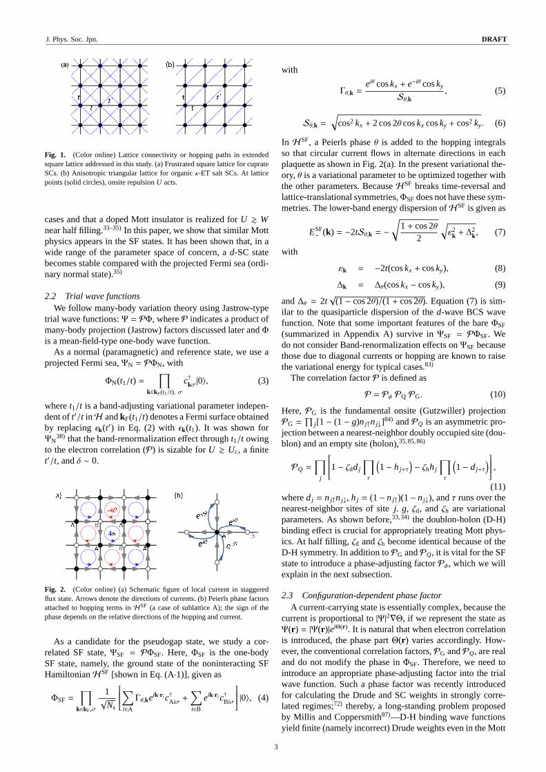
t t t'(a) (b)ttt'

Fig. 1. (Color online) Lattice connectivity or hopping paths in extendedsquare lattice addressed in this study. (a) Frustrated square lattice for cuprateSCs. (b) Anisotropic triangular lattice for organicκ-ET salt SCs. At latticepoints (solid circles), onsite repulsionU acts.

cases and that a doped Mott insulator is realized forU & Wnear half filling.33–35) In this paper, we show that similar Mottphysics appears in the SF states. It has been shown that, in awide range of the parameter space of concern, ad-SC statebecomes stable compared with the projected Fermi sea (ordi-nary normal state).35)

2.2 Trial wave functionsWe follow many-body variation theory using Jastrow-type

trial wave functions:Ψ = PΦ, whereP indicates a product ofmany-body projection (Jastrow) factors discussed later andΦ

is a mean-field-type one-body wave function.As a normal (paramagnetic) and reference state, we use a

projected Fermi sea,ΨN = PΦN, with

ΦN(t1/t) =∏

k∈kF(t1/t), σ

c†kσ|0⟩, (3)

wheret1/t is a band-adjusting variational parameter indepen-dent oft′/t inH andkF(t1/t) denotes a Fermi surface obtainedby replacingϵk(t′) in Eq. (2) with ϵk(t1). It was shown forΨN

38) that the band-renormalization effect throught1/t owingto the electron correlation (P) is sizable forU & Uc, a finitet′/t, andδ ∼ 0.

A B4θ-4θA B A

A B Aeiθe-iθ

eiθ e-iθA B A(a) (b)

Fig. 2. (Color online) (a) Schematic figure of local current in staggeredflux state. Arrows denote the directions of currents. (b) Peierls phase factorsattached to hopping terms inHSF (a case of sublattice A); the sign of thephase depends on the relative directions of the hopping and current.

As a candidate for the pseudogap state, we study a cor-related SF state,ΨSF = PΦSF. Here,ΦSF is the one-bodySF state, namely, the ground state of the noninteracting SFHamiltonianHSF [shown in Eq. (A·1)], given as

ΦSF =∏

k∈kF,σ

1√

Ns

∑i∈AΓθ,keik·r i c†Aiσ +

∑i∈B

eik·r i c†Biσ

|0⟩, (4)

with

Γθ,k =eiθ coskx + e−iθ cosky

Sθ,k, (5)

Sθ,k =√

cos2 kx + 2 cos 2θ coskx cosky + cos2 ky. (6)

In HSF, a Peierls phaseθ is added to the hopping integralsso that circular current flows in alternate directions in eachplaquette as shown in Fig. 2(a). In the present variational the-ory, θ is a variational parameter to be optimized together withthe other parameters. BecauseHSF breaks time-reversal andlattice-translational symmetries,ΦSF does not have these sym-metries. The lower-band energy dispersion ofHSF is given as

ESF− (k) = −2tSθ,k = −

√1+ cos 2θ

2

√ε2k + ∆

2k , (7)

with

εk = −2t(coskx + cosky), (8)

∆k = ∆θ(coskx − cosky), (9)

and∆θ = 2t√

(1− cos 2θ)/(1+ cos 2θ). Equation (7) is sim-ilar to the quasiparticle dispersion of thed-wave BCS wavefunction. Note that some important features of the bareΦSF

(summarized in Appendix A) survive inΨSF = PΦSF. Wedo not consider Band-renormalization effects onΨSF becausethose due to diagonal currents or hopping are known to raisethe variational energy for typical cases.83)

The correlation factorP is defined as

P = Pϕ PQ PG. (10)

Here,PG is the fundamental onsite (Gutzwiller) projectionPG =

∏j [1 − (1− g)n j↑n j↓]84) andPQ is an asymmetric pro-

jection between a nearest-neighbor doubly occupied site (dou-blon) and an empty site (holon),35,85,86)

PQ =∏

j

1− ζdd j

∏τ

(1− h j+τ

)− ζhh j

∏τ

(1− d j+τ

) ,(11)

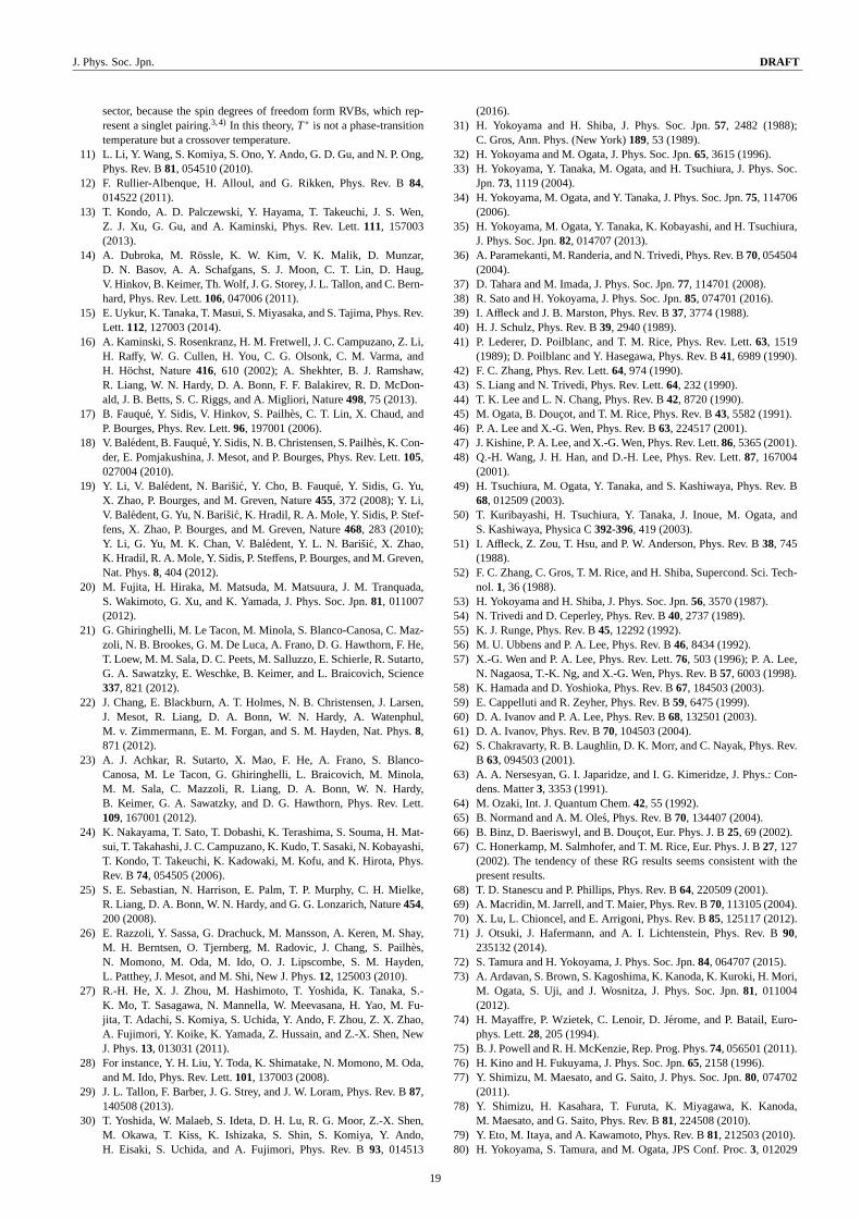
whered j = n j↑n j↓, h j = (1− n j↑)(1− n j↓), andτ runs over thenearest-neighbor sites of sitej. g, ζd, andζh are variationalparameters. As shown before,33,34) the doublon-holon (D-H)binding effect is crucial for appropriately treating Mott phys-ics. At half filling, ζd andζh become identical because of theD-H symmetry. In addition toPG andPQ, it is vital for the SFstate to introduce a phase-adjusting factorPϕ, which we willexplain in the next subsection.

2.3 Configuration-dependent phase factorA current-carrying state is essentially complex, because the

current is proportional to|Ψ|2∇Θ, if we represent the state asΨ(r ) = |Ψ(r )|eiΘ(r ). It is natural that when electron correlationis introduced, the phase partΘ(r ) varies accordingly. How-ever, the conventional correlation factors,PG andPQ, are realand do not modify the phase inΦSF. Therefore, we need tointroduce an appropriate phase-adjusting factor into the trialwave function. Such a phase factor was recently introducedfor calculating the Drude and SC weights in strongly corre-lated regimes;72) thereby, a long-standing problem proposedby Millis and Coppersmith87)—D-H binding wave functionsyield finite (namely incorrect) Drude weights even in the Mott

3


insulating regime— was solved.

Pϕyeiθ

eiϕe-iϕeiϕe-iϕ Aeiθ

H DD H A BBx

B A B B BΦSF(θ)e-iϕ e0 e-iϕ

(a) (b) (a’)Pϕ

Fig. 3. (Color online) Illustration for assigning configuration-dependentphaseϕ in Pϕ. Here, we assume that an electron hops in thex direction.For the hopping in they direction, the signs ofθ andϕ have to be reversed.The (Peierls) phase factor assigned byΦSF in hopping [Fig. 2(b)] is shown inthe blue dashed box. The values in the red boxes are the phase factors inPϕcorresponding to the three-site parts shown. The ratio (e±ϕ) indicated by redarrows is produced byPϕ in hopping.

We show that this type of phase factor also plays a vitalrole in the correlated SF state. InΦSF, a phaseθ or −θ isadded when an electron hops to a nearest-neighbor site de-pending on the direction and position (sublattice), as shownin Fig. 2(b). In the noninteracting case, such hopping occursequally in all directions. On the other hand, in the stronglycorrelated regime, the probability of hopping depends on thesurrounding configuration (see Fig. 3). For example, whena D-H pair is created [configurations (a) and (a′)], the nexthopping occurs probably in the direction in which the singlyoccupied configuration is recovered [configuration (b)]. Thishopping process does not contribute to a global current in theMott regime (U >∼ Uc).35) According to a previous study,72) toreduce the energy, it is important to cancel the phase attachedin this type of hopping (±θ) by introducing a phase parameter.

This hopping process can be specified by its local configu-rations and, correspondingly, we can attach a phase-adjustingvariational factor to the trial wave function. To be more spe-cific,Pϕ givese−iϕ as shown by the solid boxes (red) in Fig. 3,with ϕ being a variational parameter. This phase assignmentcan be written as

Pϕ = exp

[iϕ

2∑λ=1

(−1)λ+1∑

j

dλ, j

×(hλ, j+x + hλ, j−x − hλ, j+y − hλ, j−y

) ], (12)

wherex andy indicate the lattice vectors in thex andy di-rections, respectively,λ = 1 (λ = 2) indicates sublattice A(B), and j runs over all the lattice points in sublatticeλ. ByPϕ, a phase factore±iϕ is assigned to a D-H creation or anni-hilation process, in whiche∓iθ is yielded byΦSF as shown inthe dashed box (blue) in Fig. 3. Therefore, when the relationϕ = θ holds, the total phase shift in a D-H process vanishes.88)

This phase cancelation is acceptable since a phase shift doesnot appear in an exchange process in thet-J model. On theother hand, the phase is not canceled in the hopping processesunrelated to doublons (or of isolated holons).89)

The configuration-dependent phase factorPϕ is conceptu-ally distinct from position-dependent phase factors used invarious contexts.36,43,90)Note that, withoutPϕ, the energy ofthe SF state is never reduced from that ofΨN for any model

parameters, butΨSF with Pϕ has lower energy thanΨN, aswe will see below.91) Incidentally, this type of phase factorwas also recently shown to be crucial for SF states in a BoseHubbard model92) and ad-p model.93) In the regime of Mottphysics, the D-H binding affects not only the real part but alsothe phase in the wave function.

2.4 Variational Monte Carlo calculationsTo estimate variational expectation values, we adopt a plain

VMC method.94–97) In this study, we repeat linear optimiza-tion of each variational parameter with the other ones beingfixed, typically for four rounds of iteration. The linear opti-mization is convenient for obtaining an energy that is dis-continuous in some parameters (θ in this case). After con-vergence, we continue the same processes for more than 16rounds and estimate the optimized energy by averaging thedata measured in these rounds, excluding excessively scat-tered data (beyond twice the standard deviation). In each opti-mization, 2.5×105 samples are collected, so that substantiallyabout 4× 106 measurements are averaged. Only forΨSF withL = 16 andδ = 0, the sample number is reduced to 2.5×104 tosave CPU time. Typical statistical errors are 10−4t in the totalenergy and 10−4–2× 10−3 in the parameters, except near theMott transition points. We use systems ofNs = L×L sites withL = 10–18 under periodic-antiperiodic boundary conditions.

3. Staggered Flux State at Half Filling

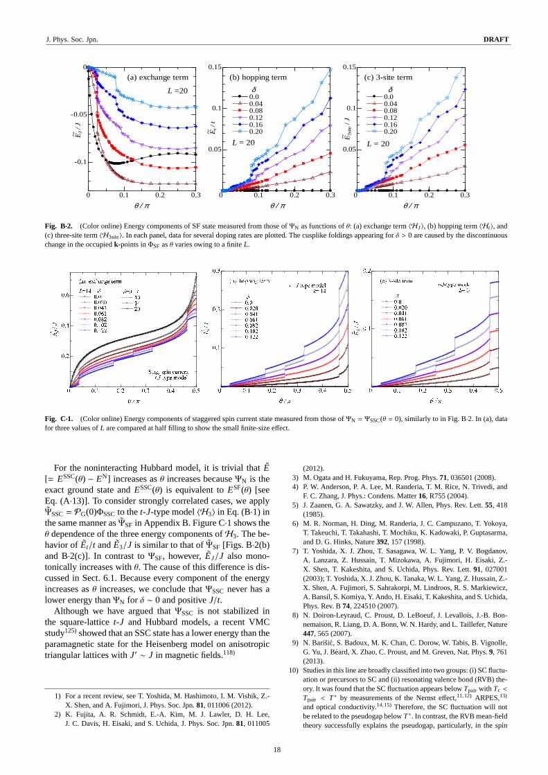
First, we study the unfrustrated cases (t′ = 0) in order tograsp the global features of the SF state because most of themdo not change even ift′ is introduced. In this section, we focuson the half-filled case.

3.1 Variational energyFigure 4(a) shows the variational energy per site ofΨSF

measured from that ofΨN,

E = ESF(θ) − EN, (13)

as a function ofθ for five values ofU/t. Here, the variationalparameters other thanθ are optimized for bothΨSF andΨN.The size dependence in the case ofU/t = 12 is also shown tosee the convergence of the values. ForU/t = 6, E monoton-ically increases as a function ofθ. This behavior is the samefor U/t = 0 shown in Fig. A·2(b) in Appendix A. Hence,ΨSF

is not stabilized for small values ofU/t. The situation changesfor U/t > 6; E/t becomes considerably negative for finiteθand has a minimum atθ/π ∼ 0.2 for large values ofU/t (= 8–16). This behavior is qualitatively consistent with that of thet-J model, the results of which are summarized in Appendix Bfor comparison. In Fig. 4(b), we plot the optimized values ofthe configuration-dependent phase factorϕ as a function ofθ.At the optimized points indicated by arrows,ϕ is very close toθ, especially for large values ofU/t. As discussed in Sect. 2.3,the Peierls phaseθ in the hopping process is mostly canceledby ϕ. Althoughθ is canceled out, the stateΨSF preserves thenature of the original flux state, as shown shortly in Sects. 3.3and 3.4. That is, a local staggered current flows and the mo-mentum distribution function has a typicalk-dependence.

Next, we discuss theU/t dependence of the energy gain ofthe fully optimizedΨSF with respect to the reference stateΨN,

∆E(SF)= E(N) − E(SF), (14)

4


-0.06-0.04-0.0200.020.04E / t

δ = 0 t' / t = 0~ U/t=12 L 10 12 14

(a) L= 10 U/t 6 6.8 8 12 16

0.1 0.2 0.3 0.4 0.50.10.20.30.4

0 θ / πφ / π

Staggered fluxδ = 0.0 t' / t = 0

L=10 U/t 6 6.8 8 12 16φ = θ(b)

Fig. 4. (Color online) (a) Variational energy per site of the staggered fluxstateΨSF (includingPϕ) measured from that ofΨN [E(θ = 0)] as a functionof θ for several values ofU/t (L = 10) in the Hubbard model at half filling.Data forL = 12 and 14 are added by dashed lines forU/t = 12. (b) Optimizedphase parameterϕ for the same values ofU/t as in (a). The line ofϕ = θ isadded for comparison. The size dependence in (b) is small. In both panels,the arrows indicate the optimal values ofθ whenE/t is minimum.

10 20 30

0.05

0.1

0.15

0U / t

∆E / t

t' / t = 0

AF d-wave Stag. flux

δ = 0

0 0.005 0.01

-0.5

-0.4

-0.3

1 / L2

E /

t

N

SF

d

AF

U / t = 8.0

1014L=18

Fig. 5. (Color online) Energy gain of AF,d-SC, and SF states with respectto projected Fermi sea (ΨN) at half filling as functions ofU/t. Data forL =14, 12, and 10 for each state are plotted as solid lines with symbols, dash-dotted lines, and dashed lines, respectively. A guide curve proportional tot/U is drawn for∆E(SF) with L = 14 (dash-dotted line). In the inset, thesystem-size dependence is shown forU/t = 8.0 and fitted by second-orderpolynomials.

whereE(N) andE(SF) are the optimized (includingθ) ener-gies per site ofΨN andΨSF, respectively. If∆E(SF) is posi-tive, the SF state is stabilized with respect toΨN. In Fig. 5,we show∆E(SF) compared with other ordered states, i.e., theAF state,ΨAF = PΦAF, and thed-SC (projected BCS) state,Ψd = PΦd. We use the sameΦAF andΦd as in the preced-

ing study (Ref. 35)98,99) but we adopt Eq. (11) forPQ. Forδ = 0 andU > Uc, Ψd is not SC but Mott insulating. InFig. 5, each state exhibits a maximum atU ∼ W (= 8t). Thesystem-size dependence of∆E for each state is large near themaximum but, as shown in the inset of Fig. 5,∆E remainsfinite and the order of the variational energy will not changeasL→ ∞. ∆E(AF) is largest, i.e., the AF state has the lowestenergy for anyU/t.33) For the SF state,∆E(SF)∼ 0 for smallvalues ofU/t (. 5). Although∆E(SF) is always smaller than∆E(d−SC), it is close to∆E(d−SC). At U/t ∼ 5, ∆E(SF)starts to increase abruptly. The range ofU/t whereΨSF is sta-bilized (U/t & 5) is similar to that ofΨd. In addition, thebehavior of physical quantities such as the momentum dis-tribution function is similar betweenΨSF andΨd as shownshortly. As mentioned, in the Heisenberg model,ΨSF(g = 0)andΨd(g = 0) are equivalent due to the SU(2) symmetry, butin the Hubbard model, the two states are not equivalent, prob-ably due to the difference in the distribution of doublons andholons.

3.2 SF transition and Mott transitionFigure 6 shows the optimizedθ andϕ in ΨSF as a function

of U/t. We find two transition points:USF/t at ∼ 4 – 5 andUc/t at ∼ 7. The former corresponds to the SF transition atwhichΨSF starts to have finiteθ andϕ and its variational en-ergy becomes lower than that ofΨN. The latter correspondsto a Mott transition at which the system starts to have a gap inthe charge degree of freedom. The symmetry does not changeatUc/t.

5 6 7 800.10.2

U / tθ /π, φ /π θ /π φ /π L 10 12 14 16

δ = 0 t' / t = 0Uc / tUSF / t10 20 3000.10.2U / t θ /π φ /π L 12 14

Fig. 6. (Color online) Optimized phase parameters (θ and ϕ) in ΨSF athalf filling. The arrows indicate the Mott transition (Uc/t) and SF transition(USF/t) for four system sizes. The inset shows the same quantities for a widerrange ofU/t, with the arrows denotingUc/t andUSF/t for L = 16.

At USF/t, θ andϕ exhibit first-order-transition-like discon-tinuities, for example, atUSF/t = 6.28 for L = 10. However,as L increases,USF/t shifts to lower values and the discon-tinuities become small and unclear, suggesting that the SFtransition is continuous and occurs at a smallU/t. Becausean appropriate scaling function is not known, we simply per-form a polynomial fit ofUSF/t up to the square of 1/L2 as arough estimate. This yieldsUSF/t = 2.93 for L = ∞ with asmall error. In any case, sinceθ andϕ are tiny forU/t . 5,we consider thatΨSF is substantially not stable in a weaklycorrelated regime.

5


5 6 7 8 9 1000.20.40.60.81

00.10.2

U / tζ

Staggered flux d ζd ζh L 10 12 14 16δ = 0.0 t' / t = 0 ddUc/t

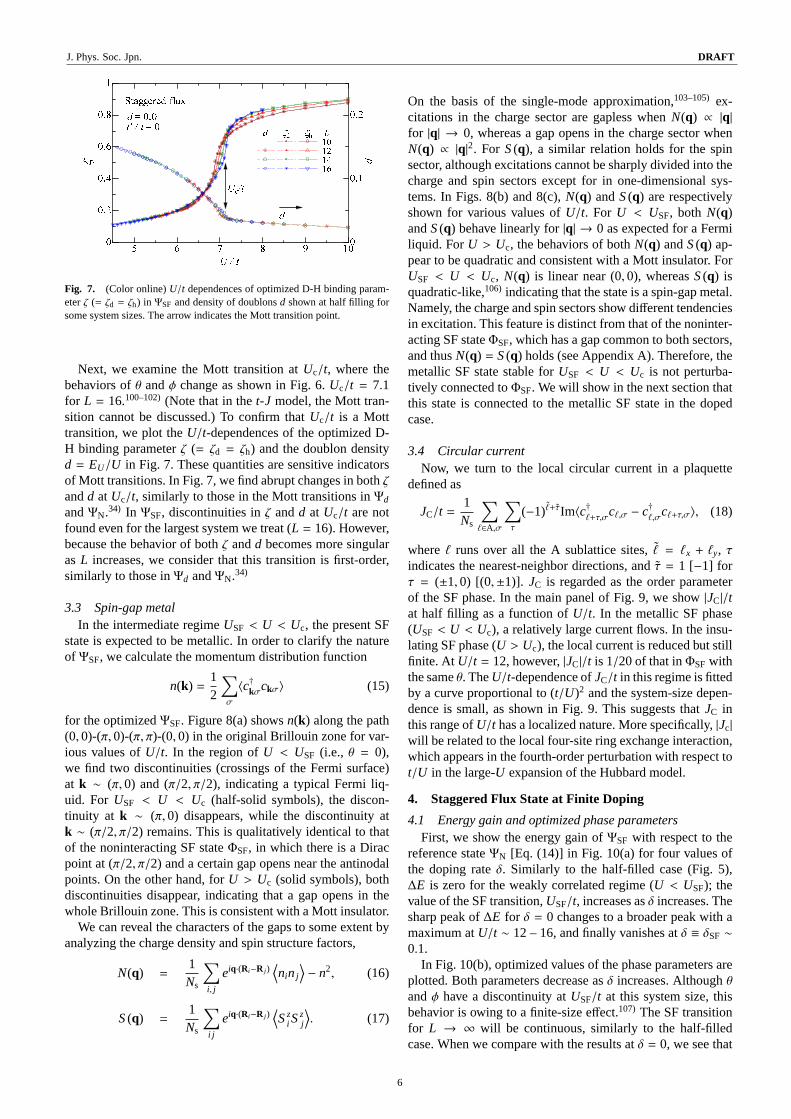
Fig. 7. (Color online)U/t dependences of optimized D-H binding param-eterζ (= ζd = ζh) in ΨSF and density of doublonsd shown at half filling forsome system sizes. The arrow indicates the Mott transition point.

Next, we examine the Mott transition atUc/t, where thebehaviors ofθ andϕ change as shown in Fig. 6.Uc/t = 7.1for L = 16.100–102)(Note that in thet-J model, the Mott tran-sition cannot be discussed.) To confirm thatUc/t is a Motttransition, we plot theU/t-dependences of the optimized D-H binding parameterζ (= ζd = ζh) and the doublon densityd = EU/U in Fig. 7. These quantities are sensitive indicatorsof Mott transitions. In Fig. 7, we find abrupt changes in bothζandd at Uc/t, similarly to those in the Mott transitions inΨd

andΨN.34) In ΨSF, discontinuities inζ andd at Uc/t are notfound even for the largest system we treat (L = 16). However,because the behavior of bothζ andd becomes more singularasL increases, we consider that this transition is first-order,similarly to those inΨd andΨN.34)

3.3 Spin-gap metalIn the intermediate regimeUSF < U < Uc, the present SF

state is expected to be metallic. In order to clarify the natureof ΨSF, we calculate the momentum distribution function

n(k) =12

∑σ

⟨c†kσckσ⟩ (15)

for the optimizedΨSF. Figure 8(a) showsn(k) along the path(0,0)-(π,0)-(π, π)-(0,0) in the original Brillouin zone for var-ious values ofU/t. In the region ofU < USF (i.e., θ = 0),we find two discontinuities (crossings of the Fermi surface)at k ∼ (π,0) and (π/2, π/2), indicating a typical Fermi liq-uid. For USF < U < Uc (half-solid symbols), the discon-tinuity at k ∼ (π,0) disappears, while the discontinuity atk ∼ (π/2, π/2) remains. This is qualitatively identical to thatof the noninteracting SF stateΦSF, in which there is a Diracpoint at (π/2, π/2) and a certain gap opens near the antinodalpoints. On the other hand, forU > Uc (solid symbols), bothdiscontinuities disappear, indicating that a gap opens in thewhole Brillouin zone. This is consistent with a Mott insulator.

We can reveal the characters of the gaps to some extent byanalyzing the charge density and spin structure factors,

N(q) =1Ns

∑i, j

eiq·(Ri−R j )⟨nin j

⟩− n2, (16)

S(q) =1Ns

∑i j

eiq·(Ri−R j )⟨Sz

i Szj

⟩. (17)

On the basis of the single-mode approximation,103–105) ex-citations in the charge sector are gapless whenN(q) ∝ |q|for |q| → 0, whereas a gap opens in the charge sector whenN(q) ∝ |q|2. For S(q), a similar relation holds for the spinsector, although excitations cannot be sharply divided into thecharge and spin sectors except for in one-dimensional sys-tems. In Figs. 8(b) and 8(c),N(q) andS(q) are respectivelyshown for various values ofU/t. For U < USF, both N(q)andS(q) behave linearly for|q| → 0 as expected for a Fermiliquid. For U > Uc, the behaviors of bothN(q) andS(q) ap-pear to be quadratic and consistent with a Mott insulator. ForUSF < U < Uc, N(q) is linear near (0,0), whereasS(q) isquadratic-like,106) indicating that the state is a spin-gap metal.Namely, the charge and spin sectors show different tendenciesin excitation. This feature is distinct from that of the noninter-acting SF stateΦSF, which has a gap common to both sectors,and thusN(q) = S(q) holds (see Appendix A). Therefore, themetallic SF state stable forUSF < U < Uc is not perturba-tively connected toΦSF. We will show in the next section thatthis state is connected to the metallic SF state in the dopedcase.

3.4 Circular currentNow, we turn to the local circular current in a plaquette

defined as

JC/t =1Ns

∑ℓ∈A,σ

∑τ

(−1)ℓ+τIm⟨c†ℓ+τ,σ

cℓ,σ − c†ℓ,σ

cℓ+τ,σ⟩, (18)

whereℓ runs over all the A sublattice sites,ℓ = ℓx + ℓy, τindicates the nearest-neighbor directions, and ˜τ = 1 [−1] forτ = (±1,0) [(0,±1)]. JC is regarded as the order parameterof the SF phase. In the main panel of Fig. 9, we show|JC|/tat half filling as a function ofU/t. In the metallic SF phase(USF < U < Uc), a relatively large current flows. In the insu-lating SF phase (U > Uc), the local current is reduced but stillfinite. At U/t = 12, however,|JC|/t is 1/20 of that inΦSF withthe sameθ. TheU/t-dependence ofJC/t in this regime is fittedby a curve proportional to (t/U)2 and the system-size depen-dence is small, as shown in Fig. 9. This suggests thatJC inthis range ofU/t has a localized nature. More specifically,|Jc|will be related to the local four-site ring exchange interaction,which appears in the fourth-order perturbation with respect tot/U in the large-U expansion of the Hubbard model.

4. Staggered Flux State at Finite Doping

4.1 Energy gain and optimized phase parametersFirst, we show the energy gain ofΨSF with respect to the

reference stateΨN [Eq. (14)] in Fig. 10(a) for four values ofthe doping rateδ. Similarly to the half-filled case (Fig. 5),∆E is zero for the weakly correlated regime (U < USF); thevalue of the SF transition,USF/t, increases asδ increases. Thesharp peak of∆E for δ = 0 changes to a broader peak with amaximum atU/t ∼ 12 – 16, and finally vanishes atδ ≡ δSF ∼0.1.

In Fig. 10(b), optimized values of the phase parameters areplotted. Both parameters decrease asδ increases. Althoughθandϕ have a discontinuity atUSF/t at this system size, thisbehavior is owing to a finite-size effect.107) The SF transitionfor L → ∞ will be continuous, similarly to the half-filledcase. When we compare with the results atδ = 0, we see that

6


00.20.40.60.81

Γ(0,0) k

n(k)

Γ(0,0) X (π,0) M(π,π)δ = 0.0 t' / t = 0 L = 14

U/t 3.0 5.0 6.0 6.5 6.9 7.2 12 16(a)

00.10.20.30.40.50.6

(0,0) q�(q)

(0,0)(π,0) (π,π)

δ = 0 t' / t = 0 L = 14 U/t 4.0 5.0 6.0 6.5 6.9 7.2 12 16(b)

00.20.40.60.81

(0,0) qS(q)

(0,0)(π,0) (π,π)

δ = 0 t' / t = 0 L = 14 U/t 3.0 4.0 5.0 6.0 6.5 6.9 7.2 12 16 USF/t ～ 5.05 Uc/t ～ 7.1 (c)00.10.20.30.4(0,0) q (π/2,0) L 10 12 14 16

L 10 12 14 16 U/t= 4.0 U/t= 6.5 Fig. 8. (Color online) Correlation functions in momentum space ofΨSF at half filling for various values ofU/t. (a) Momentum distribution function, (b)charge density structure factor, and (c) spin structure factor. In the inset in (c), the system-size dependence ofS(q) (L = 10–16) for typical cases of a Fermiliquid (U/t = 4) and spin-gap metal (U/t = 6.5) is shown for small|q| in the direction of (0,0)–(π, 0). See also Ref. 106. Open (black) symbols are forU < USF

(i.e.,θ = 0), half-solid (brown) symbols forUSF < U < Uc, and solid (red) symbols forU > Uc. For this system size (L = 14),USF/t ∼ 5.05 andUc/t ∼ 7.1.

10 20 300.10.20.30.40.5

0 U / t|JC| / t

∝(t/U)2 L 10 12 14 16δ = 0

Uc/t 10 20 300.10.20.30.40 U / t

δ 0.0 0.0278 0.0556 0.0833L = 12

USF/tFig. 9. (Color online) Absolute values of local circular current at half fill-ing as a function ofU/t for some system sizes. The SF and Mott transitionpoints are shown by arrows. A curve proportional to (t/U)2 is shown by agray dash-dotted line. The inset shows the same quantity for some dopingrates forL = 12 (discussed in Sect. 4).

ΦSF is realized in the strongly correlated region (U >W), andit is smoothly connected to the Mott insulating state at halffilling. It is also interesting thatϕ becomes larger thanθ asδincreases, while they are close to each other whenδ = 0. Thissuggests thatϕ overscreens the phaseθ in the D-H processesowing to the increasing number of free-holon processes.

Figure 11 shows theδ-dependence of∆E/t for the casewith U/t = 16. Except for the case withδ = 0, ∆E/t mono-tonically decreases as a function ofδ. Because theL depen-dence is appreciable,δSF should be somewhat larger in theL → ∞ limit. The behavior of∆E is consistent with that forthet-J model shown in Appendix B.108) In the inset of Fig. 11,theδ-dependences of the optimizedθ andϕ are plotted. Theirsystem-size dependences are very small.

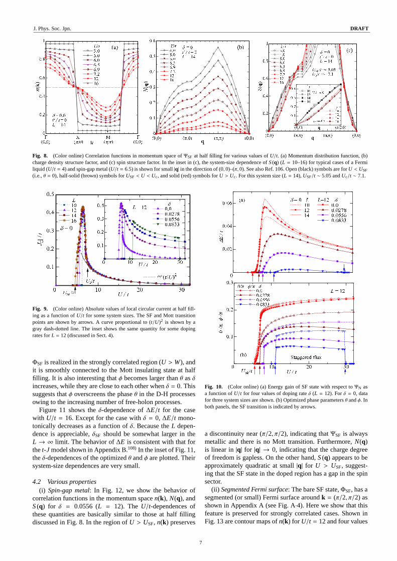
4.2 Various properties(i) Spin-gap metal: In Fig. 12, we show the behavior of

correlation functions in the momentum spacen(k), N(q), andS(q) for δ = 0.0556 (L = 12). TheU/t-dependences ofthese quantities are basically similar to those at half fillingdiscussed in Fig. 8. In the region ofU > USF, n(k) preserves

0.020.040.06

0∆E / t

L=12 δ 0.0 0.0278 0.0556 0.0833δ = 0 L 10 12 14(a)

10 20 300.10.20.3

0 U / tθ /π, φ /π Staggered flux

θ/π φ/π δ 0.0 0.0278 0.0556 0.0833 L = 12(b)USF/t

Fig. 10. (Color online) (a) Energy gain of SF state with respect toΨN asa function ofU/t for four values of doping rateδ (L = 12). Forδ = 0, datafor three system sizes are shown. (b) Optimized phase parametersθ andϕ. Inboth panels, the SF transition is indicated by arrows.

a discontinuity near (π/2, π/2), indicating thatΨSF is alwaysmetallic and there is no Mott transition. Furthermore,N(q)is linear in |q| for |q| → 0, indicating that the charge degreeof freedom is gapless. On the other hand,S(q) appears to beapproximately quadratic at small|q| for U > USF, suggest-ing that the SF state in the doped region has a gap in the spinsector.

(ii) Segmented Fermi surface: The bare SF state,ΦSF, has asegmented (or small) Fermi surface aroundk = (π/2, π/2) asshown in Appendix A (see Fig. A·4). Here we show that thisfeature is preserved for strongly correlated cases. Shown inFig. 13 are contour maps ofn(k) for U/t = 12 and four values

7


00.20.40.60.81

Γ(0,0) k

n(k)

Γ(0,0) X (π,0) M(π,π)δ = 0.0556 L = 12 t' / t = 0

U/t 4.0 6.0 7.0 7.75 8.0 10 12 16USF / t = 7.92(a) 00.10.20.30.40.50.6

(0,0) q

�(q)

(0,0)(π,0) (π,π)

δ = 0.0556 L = 12 t' / t = 0 U/t 4.0 6.0 7 7.75 8 10 12 16USF / t = 7.92

(b)

00.20.40.60.81

(0,0) q

S(q)

(0,0)(π,0) (π,π)δ = 0.0556 L = 12 t' / t = 0

U/t 4.0 6.0 7 7.75 8 10 12 16USF / t = 7.92

(c)

Fig. 12. (Color online) Behavior of (a) momentum distribution function, (b) charge density structure factor, and (c) spin structure factor ofΨSF for a finitedoping (δ = 0.0556) and various values ofU/t. Open (black) symbols are forU < USF and half-solid (brown) symbols are forU > USF. For this system size(L = 12) and doping, the SF transition is atUSF/t = 7.92.

0.05 0.1 0.150.010.020.030.040.05

0 δ∆E / t

Staggered flux∆E/t L 10 12 14 16

U / t = 160.05 0.10.10.2

0 δθ /π, φ /π θ /π φ /π L 10 12 14 16

U / t = 16φ /πθ /πFig. 11. (Color online) Energy gain of SF state with respect toΨN as afunction of doping rate atU/t = 16. Data for four system sizes are shown. Inthe inset, the optimized phase parametersθ andϕ are shown.

of δ. Here, we show the data fort′/t = −0.3 becauseΨSF isstabilized in a wide doping range (see Fig. 15 later) and thebehavior is similar to that fort′/t = 0. At half filling, there isno Fermi surface, as shown in panel (a). Upon doping, how-ever, pocket Fermi surfaces appear around (π/2, π/2) and, asδincreases, they extend to the antinodes along the AF Brillouinzone edge. These Fermi surfaces are shown by blue dashedovals in panels (b)-(d). A gap remains open near (π, 0).

(iii) Circular currents: The local circular currentsJC de-fined in Eq. (18) for the doped cases have already been shownin the inset of Fig. 9, where the evolution ofJC with increas-ing δ is shown as a function ofU/t. We find thatJC increasesasδ increases, although the optimized phase parametersθ andϕ decrease [see Fig. 10(b)]. This is probably because the num-ber of mobile carriers increases asδ increases in the stronglycorrelated regime, whose feature is typical of a doped Mottinsulator. In contrast, as shown in Appendix A,JC decreasesasδ increases in the noninteractingΦSF. At the phase tran-sition pointδSF, whereE(SF) becomes equal toE(N), the or-der parameter|JC|/t drops suddenly from 0.25–0.3 (almost themaximum value) to zero. This indicates that this transition isfirst-order, in contrast to the corresponding AF andd-SC tran-sitions, as a function ofδ.

��

��

��

�� 0.7

0.3

0.5

(a) � = 0.0

(�, �) (d) � ~ 0.12(c) � ~ 0.08

(b) � ~ 0.04

0.25

0.70.750.7 0.65

0.250.3

(�, �)

(0, 0)(�, 0)

(d) � ~ 0.12

Q = (�, �)

(c) � ~ 0.08

Fig. 13. (Color online) Contour maps of momentum distribution functionn(k) of the optimizedΨSF in the original Brillouin zone fort′/t = −0.3,U/t = 12, L = 10 – 14, and four values ofδ in (a)-(d). The wiggles of linesare simply due to the small number ofk points and are not important. The AFBrillouin zone boundary is indicated by pink dotted lines, and zone-diagonallines are shown with gray dotted lines in (c). Fermi surfaces are indicatedwith blue ovals in the third quadrants. In (d), the scattering vector ofq = Qconnecting the antinodes, discussed in Sect. 6.4, is shown with a blue arrow.

5. Effect of Diagonal Hopping t′

In this section, we study the effect of diagonal hoppingt′ inthe two cases shown in Fig. 1.

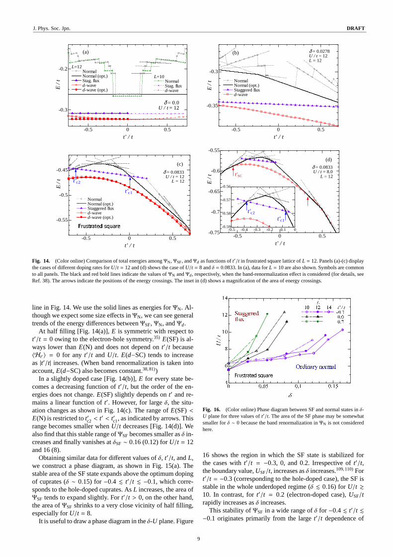
5.1 Frustrated square latticeFigure 14 summarizes the total energies ofΨSF,ΨN, andΨd

as functions oft′/t. Note that the energy forΨN without bandrenormalization exhibits complicated behaviors as a functionof t′/t. This is because the occupiedk-points in the Fermi sur-face change discontinuously inΦN. However, if we considerthe band-renormalization effect38) for ΨN and use the opti-mizedt1/t, the lowest energy forΨN becomes the black solid

8


-0.5 0 0.5

-0.3

-0.2

t' / t

E /

t

δ = 0.0 U / t = 12

L=12 Normal Normal (opt.) Stag. flux d-wave d-wave (opt.)

L=10 Normal Stag. flux d-wave

(a)

-0.5 0 0.5

-0.35

-0.3

t' / t

E /

t

δ = 0.0278 U / t = 12 L = 12

Normal Normal (opt.) Staggered flux d-wave

(b)

-0.5 0 0.5

-0.55

-0.5

-0.45

t' / t

E / t

δ = 0.0833 U / t = 12 L = 12

Normal Normal (opt.) Staggered flux d-wave d-wave (opt.)

t'c1

t'c2

(c)

��-0.5 0 0.5

-0.75

-0.7

-0.65

-0.6

-0.55

t' / t

E /

t

δ = 0.0833 U / t = 8.0 L = 12

t'c1

t'c2

t'SC

-0.5 -0.4 -0.3 -0.2 -0.1 0-0.59

-0.58

-0.57

-0.56

(d)

Fig. 14. (Color online) Comparison of total energies amongΨN,ΨSF, andΨd as functions oft′/t in frustrated square lattice ofL = 12. Panels (a)-(c) displaythe cases of different doping rates forU/t = 12 and (d) shows the case ofU/t = 8 andδ = 0.0833. In (a), data forL = 10 are also shown. Symbols are commonto all panels. The black and red bold lines indicate the values ofΨN andΨd, respectively, when the band-renormalization effect is considered (for details, seeRef. 38). The arrows indicate the positions of the energy crossings. The inset in (d) shows a magnification of the area of energy crossings.

line in Fig. 14. We use the solid lines as energies forΨN. Al-though we expect some size effects inΨN, we can see generaltrends of the energy differences betweenΨSF, ΨN, andΨd.

At half filling [Fig. 14(a)], E is symmetric with respect tot′/t = 0 owing to the electron-hole symmetry.35) E(SF) is al-ways lower thanE(N) and does not depend ont′/t because⟨Ht′⟩ = 0 for any t′/t and U/t. E(d−SC) tends to increaseas |t′/t| increases. (When band renormalization is taken intoaccount,E(d−SC) also becomes constant.38,81))

In a slightly doped case [Fig. 14(b)],E for every state be-comes a decreasing function oft′/t, but the order of the en-ergies does not change.E(SF) slightly depends ont′ and re-mains a linear function oft′. However, for largeδ, the situ-ation changes as shown in Fig. 14(c). The range ofE(SF) <E(N) is restricted tot′c2 < t′ < t′c1, as indicated by arrows. Thisrange becomes smaller whenU/t decreases [Fig. 14(d)]. Wealso find that this stable range ofΨSF becomes smaller asδ in-creases and finally vanishes atδSF ∼ 0.16 (0.12) forU/t = 12and 16 (8).

Obtaining similar data for different values ofδ, t′/t, andL,we construct a phase diagram, as shown in Fig. 15(a). Thestable area of the SF state expands above the optimum dopingof cuprates (δ ∼ 0.15) for −0.4 . t′/t . −0.1, which corre-sponds to the hole-doped cuprates. AsL increases, the area ofΨSF tends to expand slightly. Fort′/t > 0, on the other hand,the area ofΨSF shrinks to a very close vicinity of half filling,especially forU/t = 8.

It is useful to draw a phase diagram in theδ-U plane. Figure

0 0.05 0.1 0.1546810

1214

δU / t

L 10 12 14 t' / t -0.3 0.0 0.2Frustrated square Ordinary normalStaggered flux

Fig. 16. (Color online) Phase diagram between SF and normal states inδ-U plane for three values oft′/t. The area of the SF phase may be somewhatsmaller forδ ∼ 0 because the band renormalization inΨN is not consideredhere.

16 shows the region in which the SF state is stabilized forthe cases witht′/t = −0.3, 0, and 0.2. Irrespective oft′/t,the boundary value,USF/t, increases asδ increases.109,110)Fort′/t = −0.3 (corresponding to the hole-doped case), the SF isstable in the whole underdoped regime (δ . 0.16) for U/t &10. In contrast, fort′/t = 0.2 (electron-doped case),USF/trapidly increases asδ increases.

This stability ofΨSF in a wide range ofδ for −0.4 . t′/t .−0.1 originates primarily from the larget′/t dependence of

9


0 0.05 0.1 0.15-0.50

0.5

δt' / t

L=10 12 14 U / t 8 12 16Ordinary normalStaggered flux Ordinary normalhole dopedelectron doped Frustrated square(a) 0 0.05 0.1-1

01

δt' / t L=10 12 U / t 8 12

Ordinary normalStaggered fluxκ-ET salts Aniso. triangular

(b)Fig. 15. (Color online) Phase diagrams in theδ-t′ plane with doping rate (δ) and frustration strength (t′/t) for (a) the frustrated square lattice and (b) theanisotropic triangular lattice forU/t = 8 and 12 [and 16 in (a)]. “Ordinary normal” indicates the projected Fermi sea. The symbols with vertical bars placed att′/t ∼ −0.25 indicate that the SF state is not stabilized at these values ofδ. The scale of the abscissa is identical in the two panels.

ΨN and the very smallt′/t dependence ofΨSF. This meansthat the nature ofΨSF for t′ = 0 quantitatively remains that fort′/t , 0. For example, we show in Fig. 17 thet′/t dependencesof the optimized phase parameters and local circular current,JC, which do not strongly depend ont′/t. Furthermore, weconfirm that the momentum distribution functionn(k) is al-most the same fort′/t , 0. Note that this is in sharp contrast tothed-SC state, in whichn(k) in the antinodal region markedlychanges witht′/t (see Fig. 29 in Ref. 35). The reason for thisdifference betweenΨSF andΨd will be as follows. SinceΨSF

is very appropriately defined for the simple square lattice,t′

change the wave function ofΨSF only slightly. On the otherhand,Ψd has a gap opening at the Fermi surface near (π,0),which is markedly affected byt′. In this context, it is naturalto expect that extra current, such as diagonal currents in chiralspin states,111) will not be favored.83)

-0.6 -0.4 -0.2 0 0.200.10.20.30.4

00.10.2

t' / t|JC| / t U / t = 12 L = 12

Frustrated squareθ /π, φ /π|JC| / tφ /πθ /π metastable

|JC|/t θ /π φ /π δ 0.0833 0.1111

Fig. 17. (Color online)t′/t dependences of the optimized phase parametersθ andϕ and the local circular currentJC in ΨSF for two values ofδ. Theunstable regions ofΨSF are indicated by gray dashed lines and “metastable”.

In many studies on thet-J and Hubbard models, the insta-bility toward phase separation near half filling has been dis-cussed. Recently, states with AF long-range orders have beenshown to be unstable toward phase separation fort′/t ∼ 0 forthe Hubbard model using the VMC method.35,38,112–114)Forthet-J model, an SF state has also been shown to be unstabletoward phase separation in a wide range ofδ for t′/t = 0.61)

Therefore, we need to check this instability in the present

0 0.1 0.2

-10

0

10

δ

χ c-1

Stag. flux

U/t, t'/t, L 12 0.3 12 16 0 14 12 0 12 12 0 14 12 -0.3 10 12 -0.3 12 12 -0.3 14

d-wave U/t, t'/t, L

12 0 12 12 -0.3 12

Fig. 18. (Color online) Inverse charge susceptibility of the SF state shownas a function of doping rateδ for some parameter sets for the frustrated squarelattice [Fig. 1(a)]. We add guide lines (thick dashed) fort′/t = 0 and−0.3(U/t = 12, L = 14). The same quantity of thed-SC state is also shown withhalf-solid green symbols for comparison. Zigzags of the data forΨSF are dueto the discontinuous change in the occupiedk points and other finite-sizeeffects.

case. To this end, we consider the charge compressibilityκ orequivalently the charge susceptibilityχc (= n2κ), the inverseof which is given as

χ−1c =

∂2E(n)∂n2

∼ N2s

E(N + 4)+ E(N − 4)− 2E(N)42

, (19)

with n = N/Ns. If χ−1c < 0, the system is unstable toward

phase separation. In Fig. 18, we show theδ dependence ofχ−1

c for three values oft′/t andL. We find thatχ−1c is basically

negative fort′/t = 0 and 0.3, indicating thatΨSF is unstabletoward phase separation (data points ofδ ∼ 0 should be dis-regarded because they are affected by the Mott singularity atδ→ 0). This result is consistent with the previous one for thet-J model fort′/t = 0.61) In contrast, fort′/t = −0.3, χ−1

c be-comes positive forδ & 0.05 and comparable to that ofd-SC(green symbols). Therefore, a homogeneous SF state is possi-ble for the parameters of hole-doped cuprates.

10


5.2 Anisotropic triangular latticeFor the anisotropic triangular lattice, Fig. 19 summarizes

the total energies ofΨSF, ΨN, andΨd as a function oft′/t.Again,E(N), the lowest energy ofΨN considering band renor-malization,38) is shown by the black solid lines. First, letus consider the half-filled case [Fig. 19(a)].E is symmetricwith respect tot′/t = 0 owing to the electron-hole symme-try.35) Similarly to the case on the frustrated square lattice,E(FS) andE(d−SC) (if the band renormalization is consid-ered115,116)) are constant. For the ground state, we find fromFig. 19(a) thatΨN has a lower energy thanΨd for t′ > t′SC witht′SC/t = 0.807 forL = 12. However, the (π, π)-AF state or in-commensurate AF states including the case of a 120◦ structurehas a lower energy at half filling.115–117)

0 0.2 0.4 0.6 0.8-0.45

-0.4

-0.35

t' / t

E /

t

δ = 0.0 U / t = 8.0

L=10 12 Normal Stag. flux d-wave

(a)

d (renorm.) t'c2�� t'SC

t'c0Normal(opt.)

-1 -0.5 0 0.5

-0.42

-0.4

-0.38

-0.36

t' / t

E /

t

δ = 0.0556 U / t = 12 L = 12

Normal Stag. flux d-wave

t'c1

t'c2

(b)

Fig. 19. (Color online) Comparison of total energy amongΨN, ΨSF, andΨd as functions oft′/t. Panel (a) displays the half-filled case forU/t = 8(only the data fort′/t ≥ 0 are shown) andL = 10 and 12, and (b) a doped casefor U/t = 12 (δ = 0.0556) andL = 12. We show the optimized values by theband renormalization forΨN with (black) solid lines. The band-renormalizeddata forΨd are also shown in (a) with a (red) solid line.

We compare the energies betweenΨN andΨSF, assumingthat AF states are not stabilized. In Fig. 19(a),ΨSF is morestable thanΨN for t′ < t′c2 with t′c2/t = 0.749 (0.763) forU/t = 8 andL = 12 (10). We employ the valueU/t = 8 sim-ply because it is frequently used as a plausible value forκ-ETsalts.73) Actually,ΨSF is Mott insulating atU/t = 8; a value ofU/t . 7.1 is necessary for a metallic state. However, the pointhere does not change qualitatively irrespective of whetherΨSF

is insulating or metallic. On the basis of similar calculationsfor various values ofU/t and t′/t, we construct a phase dia-gram within the SF and normal state at half filling (Fig. 20),which is relevant for organic conductors. The boundary value

USF/t betweenΨSF andΨN increases ast′/t increases.As shown before, the Mott transition occurs atUc ∼ 7.1t

for t′ = 0. Since the properties ofΨSF are similar to the caseof t′ = 0, the SF state is metallic forU . Uc and insulatingfor U > Uc. This phase boundary is also shown in Fig. 20.

0 0.5 1 1.5

4

6

8

10

12

t' / t

U /

t

Staggered flux

Ordinary normal

�� δ = 0.0

t'c0 t'SF L 10 12 14

t1 = 0

t1�0

Uc/t

Fig. 20. (Color online) Phase diagram between the SF and normal states int′-U plane at half filling on anisotropic triangular lattice. Boundaries (USF,solid lines) are determined for three system sizes. The green arrow near thevertical axis represents the range of the metallic SF state. The dashed linesshow the boundary inΨN regarding whether the nesting condition is restored(t1 = 0) or not (t1 , 0) in the renormalized band (see Sect. 6.2 later).

For a doped case, we show in Fig. 19(b) thet′/t dependenceof the total energy for the three states for typical parameters.It is noteworthy thatE/t for ΨN andΨd decreases rapidly forlarge values of|t′/t| (∼ 1). Obtaining similar data for variousvalues oft′/t andδ, we construct a phase diagram in theδ-t′

space [Fig. 15(b)]. Compared with the case of the frustratedsquare lattice [Fig. 15(a)], the area ofΨSF is restricted to thesmall doping region.

6. Discussion

6.1 Phase cancelation mechanismFirst, let us consider intuitively whyΨSF has a low energy

in the strongly correlated region of the Hubbard model. Asdiscussed in a previous study,35) the processes correspondingto theJ term in thet-J model are those in which a D-H pairis created or annihilated as shown in Fig. 21(a). Generallyspeaking, the phase yielded in this process causes a loss ofkinetic energy. In order to reduce this kinetic energy loss, thephaseθ should be eliminated by the phaseϕ by applyingPθwith ϕ ∼ θ in the same manner as introduced in Ref. 72.

We expect a similar phenomenon in the Heisenberg inter-action in thet-J model. In theJ term, an↑ spin at sitei hops tosite j (= i+τ) and simultaneously a↓ spin at sitej hops to sitei. As shown in Fig. 21(b), if the former hopping yields a phaseθ, the latter yields−θ in ΦSF; the total phase in the exchangeprocess precisely cancels out (shown in the square brackets inFig. 21). Since the two processes occur simultaneously, it isunnecessary to introduceϕ in thet-J model to stabilize the SFstate. On the other hand, in the Hubbard model [Fig. 21(a)],a hopping resulting in D-H-pair annihilation does not neces-sarily occur immediately after a D-H pair is created; thesetwo processes are mutually independent events. Therefore, itis necessary to introduce the phaseϕ to eliminate±θ in eachprocess in order to stabilize the SF state.

11


ei(θ-ϕ)e-i(θ-ϕ)

eiθe-iθ

eiθeiθ

(a) ΨSF (Hubbard) (b) ΨSF (t - J) (c) ΨSSC (t - J)D-H process exhange exchange[~ ei0] [= ei0] [= e2iθ]i j

~ ~

Fig. 21. (Color online) Illustration of phase factors added in (a) creationor annihilation process of doublon-holon (D-H) pair inΨSF for large-U/tHubbard model, (b) spin exchange process inΨSF for t-J model, and (c) spinexchange process inΨSSC for t-J model. For details, see text.

Finally, let us apply the present mechanism to the spin-current-carrying state. Staggered spin current (SSC) states (orsometimes called spin-nematic states63)) have been consid-ered to be candidates for hidden orders in various systems.118)

In these states, counter-rotating currents of↑ and↓ spins al-ternately flow in each plaquette [Fig. A·1(b)]. We have car-ried out similar VMC calculations for the projected SSC stateΨSSC= PG(0)ΦSSC. The results are summarized in AppendixC. We conclude thatΨSSC is not stabilized for anyJ/t and un-derdopedδ. We can easily see the reason for this by consid-ering the phase cancelation. As we can see from Fig. 21(c),the total phase added in an exchange process inΨSSC re-mains 2θ. We found that this phase is difficult to eliminateby configuration-dependent phase factors such asPϕ. There-fore, we conclude that the SSC state or spin-nematic state willnever be stabilized.

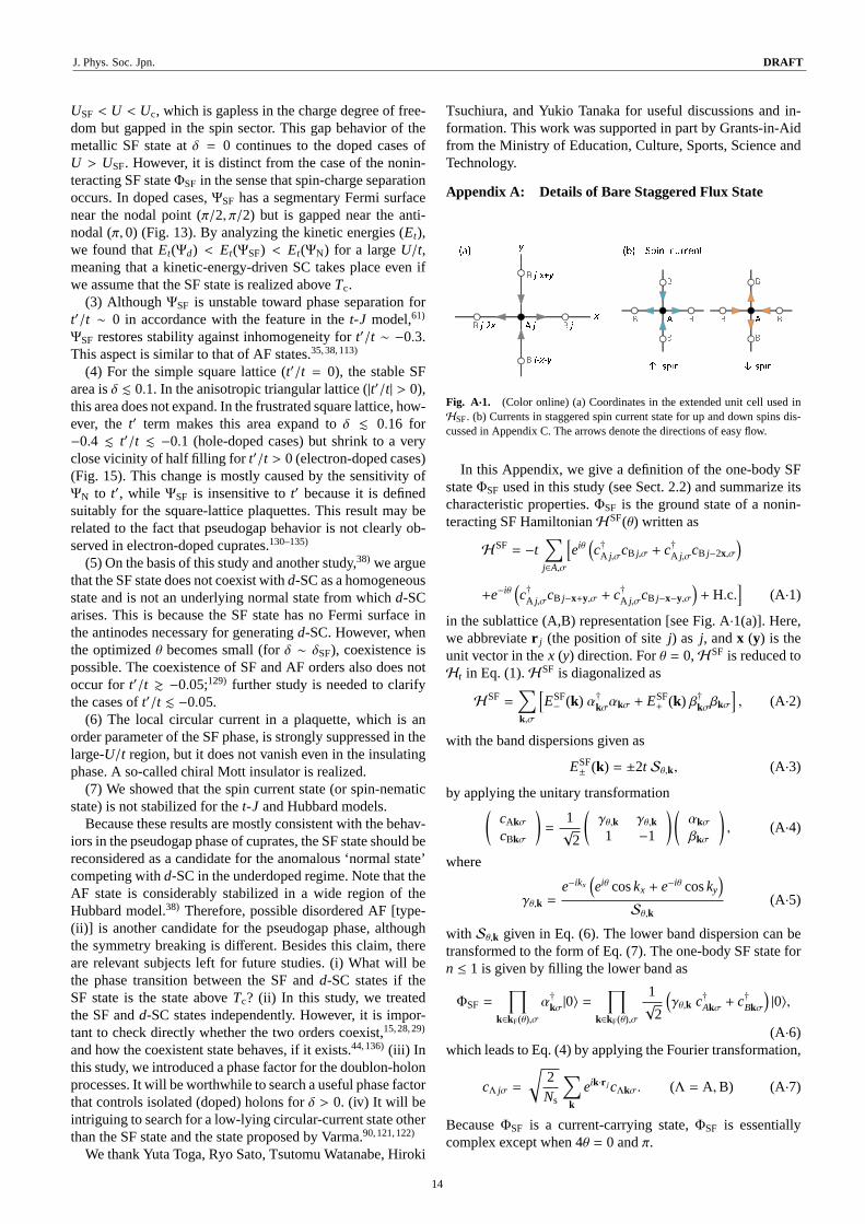
6.2 Kinetic energy gainWe discuss another physical reason for the stabilization of

the SF state. In Fig. 22. we show the difference in the kineticenergy∆Et and interaction energy∆EU between the optimalSF state and the projected Fermi sea,

∆Et = Et(N) − Et(SF),∆EU = EU(N) − EU(SF), (20)

for four values ofδ. In previous papers, we perfomed the sameanalysis forΨd andΨN,33,34) and showed that the SC transi-tion is driven by the kinetic energy gain forU & Uco withUco/t being the crossover value from weakly to strongly cor-related regimes. In Fig. 22, we find that a similar phenomenonemerges betweenΨSF andΨN: Kinetic energy gain occurs inthe strongly correlated region. The physical reason for thiswill be as follows. In the strongly correlated regime, the ki-netic energy is dominated by the D-H pair creation or annihi-lation processes (not shown). Since the phases arising in theseprocesses are canceled out byϕ, this kinetic energy gain cor-responds to that in theJ-term in thet-J model.

In Fig. 23. we show a similar comparison between thed-SCand optimal SF states, i.e.,

∆Et = Et(SF)− Et(d−SC),∆EU = EU(SF)− EU(d−SC). (21)

In particular, in the regime ofU > Uc(SF) at half filling andU > USF for δ > 0, the energy gain occurs exclusively inthe kinetic part (∆Et > 0 and∆EU < 0). Thus, the causeof stabilization both inΨN → ΨSF and inΨSF → Ψd is the

-0.3-0.2-0.100.1

∆Et / t L=12 δ 0.0 0.0278 0.0556 0.0833(a)

δ = 0 L 10 12 14

0 10 20 30-0.100.10.20.3

U / t∆EU / t

L=12 δ 0.0 0.0278 0.0556 0.0833(b) δ = 0 L 10 12 14

Fig. 22. (Color online) The two components of the energy difference be-tween the SF state and the projected Fermi sea are shown for some dopingrates (t′/t = 0, U/t = 12): (a) kinetic energy and (b) interaction energy parts.For δ = 0, we add data forL = 10 and 14. The arrows indicateUSF/t forL = 12.

kinetic energy gain for a sufficiently largeU/t.119)

6.3 Comparison with experiments(i) High-Tc cuprates: Here, we discuss the lattice trans-

lational symmetry, which is broken in the present SF state.The peaks arising from local loop currents in the polarizedneutron scattering spectra are found atk = (0,0),17–19) sug-gesting that the lattice translational symmetry is preservedin the pseudogap phase. Some authors have argued that theSF state breaks this symmetry, but physical quantities calcu-lated with SF states display a (0,0) peak in addition to a (π, π)peak.120) The above neutron experiments appear to be consis-tent with more complicated circular-current states that do notbreak this symmetry.90,121,122)Recently, however, one of theauthors showed that this type of circular-current state is notstabilized with respect to the normal state in a wide range ofthe model parameters on the basis of systematic VMC cal-culations with refined wave functions ford-p-type models.Instead, SF states are stabilized in some parameter ranges.123)

On the other hand, the shadow bands observed in the ARPESspectra,24–27) which also characterize the pseudogap phase,seem to require the scattering of (π, π) and a folded Brillouinzone. Therefore, the issue of translational symmetry breakingis still controversial.

(ii) Organic conductors: In Sect. 5.2, we studied theanisotropic triangular lattice. Let us here discuss the rele-vance of the present results to experiments. As discussed inSect. 1, deuteratedκ-(ET)2Cu[N(CN)2]Br has t′/t ∼ 0.4.The present results show that the SF state is stabilized forthe case oft′/t ∼ 0.4. Therefore, the pseudogap behaviorfor T > Tc observed in deuteratedκ-(ET)2Cu[N(CN)2]Bris probably caused by the SF state. On the other hand,κ-

12


-0.2-0.10∆Et / t ∆E = ESF - Ed(a)

10 20 300.010.020.030 U / t∆E / t δ = 0 L 10 12 14Uc/t (d)

Uc/t (SF)USF/t

0 10 20 3000.10.2

U / t∆EU / t

(b) L=12 δ 0 0.0278 0.0556 0.0833δ = 0 L 10 12 14

Fig. 23. (Color online) The two components of the energy difference be-tween thed-SC and SF states are shown for some doping rates (t′/t = 0,L = 12): (a) kinetic energy and (b) interaction energy parts. The symbols arecommon to all panels. Forδ = 0, data forL = 10 and 14 are added. Thearrows indicateUSF/t in the SF state forδ > 0. The inset in (a) shows thedifference in total energy (∆E = ∆Et + ∆EU ) for four values ofδ.

(ET)2Cu2(CN)3 with t′/t ∼ 0.8 shows Fermi-liquid-like be-havior aboveTc. Since the present result shows that the SFstate is not stabilized for the case oft′/t ∼ 0.8, the normalstate ofκ-(ET)2Cu2(CN)3 is naturally understood on the basisof ΨN. Although our results are consistent with experiments,quantitative discussions will be necessary to determine the ef-fective value ofU/t as well ast′/t more accurately for eachcompound.124,125)

For the organic conductors with finite doping, we find thatΨSF is not stabilized atδ = 0.11 for bothU/t = 8 and 12, re-gardless of the value oft′/t. Thus, concerning the pseudogapphenomena found in a dopedκ-ET salt,79) we cannot concludethat the SF state is a candidate for the pseudogap phase. Otherfactors may be necessary to understand this pseudogap.

6.4 Related studies and coexistence with other ordersA decade ago, Yang, Rice, and Zhang introduced a phe-

nomenological Green’s function that can represent vari-ous anomalous properties of the pseudogap phase.126) TheirGreen’s function contains a self-energy that reproduces thedx2−y2-wave RVB state at half filling. For finite doping, theGreen’s function is assumed to have the same self-energy butwithout the features of SC. On the other hand, the SF stateused in the present paper is also connected to thedx2−y2-waveRVB state due to the SU(2) symmetry at half filling. For finitedoping, however, the SF state does not show SC. Therefore,we expect a close relationship between the present SF stateand the phenomenological Green’s function, although the ex-plicit correspondence is not known.

As mentioned in Sect. 1, an AF state was recently studiedby applying a VMC method with a band-renormalization ef-fect to the Hubbard model on the frustrated square lattice.38)

It revealed that the AF state is considerably stable and occu-pies a wide range of the ground-state phase diagram. In dopedmetallic cases fort′/t . −0.05, an AF state called type-(ii) AFstate is stabilized, while fort′/t & −0.05, a type-(i) AF stateis stabilized. In a type-(ii) AF state, a pocket Fermi surfacearises around (π/2, π/2) and a gap opens in the antinode [near(π,0)]. As δ increases, the Fermi surface around (π/2, π/2)extends toward the antinodes along the AF Brillouin zoneedge. Such behavior resembles the pseudogap phenomena,as the SF state treated in this paper does. Thus, if such fea-tures are preserved when the AF long-range order is brokeninto a short-range order for some reason, as actually observedin cuprates,127) a (disordered) type-(ii) AF state becomes an-other candidate for a pseudogap state, although the symmetrybreaking is rather different from that in the SF state.

Let us discuss the coexistence withd-SC. The samestudy38) as discussed above showed that, although type-(ii)AF states do not coexist withd-SC, metallic AF states fort′/t & −0.05 [called type-(i) AF] coexist withd-SC; thesetype-(i) AF states have pocket Fermi surfaces in the antin-odes. This corroborates the fact that the electron scatteringof q = (π, π) that connects two antinodes is crucial for theappearance ofd-SC. From this result, we expect that the SFstate is unlikely to coexist withd-SC because gaps open inthe antinodes in the SF state, as shown in Fig. 13(d). As anexception, coexistence may be possible forδ ∼ δSF, wherethe Fermi surfaces extend to the antinodes, as discussed inRef. 38. Thus, the SF order probably competes with thed-SCorder rather than underlies it.128) We need to directly confirmthis by examining a mixed state of the SF andd-SC orders.

Finally, we consider the possibility of the coexistence of AFand SF orders. Recently, a Hubbard model with an SF phase,namely,H = HSF+HU [see Eqs. (1) and (A·1)], was studiedusing a VMC method with a mixed state of SF and AF orders,ΨSF+AF.129) For θ = 0 [Eq. (1) with t′ = 0], the optimizedΨSF+AF is reduced toΨAF, which belongs to the type-(i) AFphase. Namely, the SF order is excluded by the type-(i) AForder. This is probably because the AF order is energeticallydominant over the SF order, and the loci of Fermi surfacescompete with each other.

7. Conclusions

In this paper, we studied the stability and other propertiesof the staggered flux (SF) state in the two-dimensional Hub-bard model at and near half filling. We carried out systematiccomputations forU/t, t′/t, andδ, using a variational MonteCarlo method, which is useful for treating correlated systems.In the trial SF state, a configuration-dependent phase factorwas introduced, which is vital to treat a current-carrying statein the regime of Mott physics. In this SF state, we found agood possibility of explaining the pseudogap phenomena inhigh-Tc cuprates andκ-ET salts. The main results are summa-rized as follows:

(1) The SF state is not stabilized in a weakly correlatedregime (U/t . 5), but becomes considerably stable in astrongly correlated regime [Figs. 5 and 10(a)]. The physicalproperties in the latter regime are consistent with those of thet-J model.32,43,44,60)The transition fromΨN to ΨSF at USF/tis probably continuous.

(2) At half filling (δ = 0), the SF state becomes Mott in-sulating forU > Uc ∼ 7t. A metallic SF state is realized for

13


USF < U < Uc, which is gapless in the charge degree of free-dom but gapped in the spin sector. This gap behavior of themetallic SF state atδ = 0 continues to the doped cases ofU > USF. However, it is distinct from the case of the nonin-teracting SF stateΦSF in the sense that spin-charge separationoccurs. In doped cases,ΨSF has a segmentary Fermi surfacenear the nodal point (π/2, π/2) but is gapped near the anti-nodal (π,0) (Fig. 13). By analyzing the kinetic energies (Et),we found thatEt(Ψd) < Et(ΨSF) < Et(ΨN) for a largeU/t,meaning that a kinetic-energy-driven SC takes place even ifwe assume that the SF state is realized aboveTc.

(3) AlthoughΨSF is unstable toward phase separation fort′/t ∼ 0 in accordance with the feature in thet-J model,61)

ΨSF restores stability against inhomogeneity fort′/t ∼ −0.3.This aspect is similar to that of AF states.35,38,113)

(4) For the simple square lattice (t′/t = 0), the stable SFarea isδ . 0.1. In the anisotropic triangular lattice (|t′/t| > 0),this area does not expand. In the frustrated square lattice, how-ever, thet′ term makes this area expand toδ . 0.16 for−0.4 . t′/t . −0.1 (hole-doped cases) but shrink to a veryclose vicinity of half filling fort′/t > 0 (electron-doped cases)(Fig. 15). This change is mostly caused by the sensitivity ofΨN to t′, while ΨSF is insensitive tot′ because it is definedsuitably for the square-lattice plaquettes. This result may berelated to the fact that pseudogap behavior is not clearly ob-served in electron-doped cuprates.130–135)

(5) On the basis of this study and another study,38) we arguethat the SF state does not coexist withd-SC as a homogeneousstate and is not an underlying normal state from whichd-SCarises. This is because the SF state has no Fermi surface inthe antinodes necessary for generatingd-SC. However, whenthe optimizedθ becomes small (forδ ∼ δSF), coexistence ispossible. The coexistence of SF and AF orders also does notoccur for t′/t & −0.05;129) further study is needed to clarifythe cases oft′/t . −0.05.

(6) The local circular current in a plaquette, which is anorder parameter of the SF phase, is strongly suppressed in thelarge-U/t region, but it does not vanish even in the insulatingphase. A so-called chiral Mott insulator is realized.

(7) We showed that the spin current state (or spin-nematicstate) is not stabilized for thet-J and Hubbard models.

Because these results are mostly consistent with the behav-iors in the pseudogap phase of cuprates, the SF state should bereconsidered as a candidate for the anomalous ‘normal state’competing withd-SC in the underdoped regime. Note that theAF state is considerably stabilized in a wide region of theHubbard model.38) Therefore, possible disordered AF [type-(ii)] is another candidate for the pseudogap phase, althoughthe symmetry breaking is different. Besides this claim, thereare relevant subjects left for future studies. (i) What will bethe phase transition between the SF andd-SC states if theSF state is the state aboveTc? (ii) In this study, we treatedthe SF andd-SC states independently. However, it is impor-tant to check directly whether the two orders coexist,15,28,29)

and how the coexistent state behaves, if it exists.44,136)(iii) Inthis study, we introduced a phase factor for the doublon-holonprocesses. It will be worthwhile to search a useful phase factorthat controls isolated (doped) holons forδ > 0. (iv) It will beintriguing to search for a low-lying circular-current state otherthan the SF state and the state proposed by Varma.90,121,122)

We thank Yuta Toga, Ryo Sato, Tsutomu Watanabe, Hiroki

Tsuchiura, and Yukio Tanaka for useful discussions and in-formation. This work was supported in part by Grants-in-Aidfrom the Ministry of Education, Culture, Sports, Science andTechnology.

Appendix A: Details of Bare Staggered Flux State

A j B j(a)

B j-2x B j-x-yB j-x+yy

x B BBA B

(b) Spin currentB B

BA B↑- spin ↓-spin

Fig. A·1. (Color online) (a) Coordinates in the extended unit cell used inHSF. (b) Currents in staggered spin current state for up and down spins dis-cussed in Appendix C. The arrows denote the directions of easy flow.

In this Appendix, we give a definition of the one-body SFstateΦSF used in this study (see Sect. 2.2) and summarize itscharacteristic properties.ΦSF is the ground state of a nonin-teracting SF HamiltonianHSF(θ) written as

HSF = −t∑j∈A,σ

[eiθ

(c†A j,σcB j,σ + c†A j,σcB j−2x,σ

)+e−iθ

(c†A j,σcB j−x+y,σ + c†A j,σcB j−x−y,σ

)+ H.c.

](A·1)

in the sublattice (A,B) representation [see Fig. A·1(a)]. Here,we abbreviater j (the position of sitej) as j, andx (y) is theunit vector in thex (y) direction. Forθ = 0,HSF is reduced toHt in Eq. (1).HSF is diagonalized as

HSF =∑k,σ

[ESF− (k) α†kσαkσ + ESF

+ (k) β†kσβkσ

], (A·2)

with the band dispersions given as

ESF± (k) = ±2t Sθ,k , (A·3)

by applying the unitary transformation(cAkσ

cBkσ

)=

1√

2

(γθ,k γθ,k1 −1

) (αkσ

βkσ

), (A·4)

where

γθ,k =e−ikx

(eiθ coskx + e−iθ cosky

)Sθ,k

(A·5)

with Sθ,k given in Eq. (6). The lower band dispersion can betransformed to the form of Eq. (7). The one-body SF state forn ≤ 1 is given by filling the lower band as

ΦSF =∏

k∈kF(θ),σ

α†kσ|0⟩ =∏

k∈kF(θ),σ

1√

2

(γθ,k c†Akσ + c†Bkσ

)|0⟩,

(A·6)which leads to Eq. (4) by applying the Fourier transformation,

cΛ jσ =

√2Ns

∑k

eik·r j cΛkσ. (Λ = A,B) (A·7)

BecauseΦSF is a current-carrying state,ΦSF is essentiallycomplex except when 4θ = 0 andπ.

14


-0.8-0.6-0.4-0.20E / t δ 0 0.1 0.2 0.3 0.4 0.5U / t = 0SF model~

(a)

0.1 0.2 0.3 0.4 0.50.511.5

0 θ / πE / t U / t = 0Hubbard model

Analytic δ = 0 VMC δ = 0 L 10 20 δ = 0.08 20~(b)

Fig. A·2. (Color online) Total energies per site ofΦSF measured from thatof ΦN [Eq. (A·8)] are drawn as functions ofθ for (a) the SF Hamiltonian[Eq. (A·1)] and (b) the Hubbard Hamiltonian [Eq. (1)]. In (a), Eqs. (A·10)and (A·12) are used with a commonθ in ΦSF andHSF as the ground state.In (b), Eqs. (A·9) and (A·11) are used withθ being varied inΦSF; we plotVMC data for some cases in addition to the analytic result at half filling. Weconfirmed thatP has almost no effect forU = 0. t′ is fixed at 0.

The total energy per site ofΦSF measured from that of thebare Fermi seaΦN is written as

E = ESF− EN. (A·8)

Here,EN for ΨN is obtained for the Hubbard model [Eq. (1)with U = 0] through

EN =1Ns

⟨ΦN|Ht |ΦN⟩⟨ΦN|ΦN⟩

=1Ns

∑k∈kF(θ=0),σ

εk , (A·9)

whereεk [Eq. (8)] is the bare dispersion of an ordinary Fermisea, andEN is obtained for the SF model [Eq. (A·1)] through

EN =1Ns

⟨ΦN|HSF|ΦN⟩⟨ΦN|ΦN⟩

=1Ns

∑k∈kF(θ=0),σ

ESF− (k). (A·10)

The energy ofΦSF for the Hubbard model is given by

ESF =⟨ΦSF|Ht |ΦSF⟩Ns⟨ΦSF|ΦSF⟩

= −2t cosθNs

∑k∈kF(θ),σ

(coskx + cosky

)2

Sθ,k,

(A·11)and that for the SF Hamiltonian is given by

ESF =1Ns

⟨ΦSF|HSF|ΦSF⟩⟨ΦSF|ΦSF⟩

=1Ns

∑k∈kF(θ),σ

ESF− (k). (A·12)

In Fig. A·2(a), we showE/t for HSF as a function ofθ. Be-causeΦSF is the exact ground state ofHSF, E/t ≤ 0 holds; athalf filling, ESF andEN are identical because the Fermi sur-faces ofΦN andΦSF are identical, but the energy ofΦSF issizably reduced asδ or θ increases. In contrast, for the Hub-

bard model withU = 0 (Ht), E/t is positive because the exactground state ofHt isΦN [ΦSF(θ = 0)]. E/t monotonically in-creases asθ increases, as shown in Fig. A·2(b). Forθ ∼ 0, ESF

in Eq. (A·11) increases quadratically as

ESF = EN + θ2t

∑k∈kF (θ),σ

(coskx − cosky

)2∣∣∣coskx + cosky

∣∣∣ + · · · , (A·13)

at least forδ = 0. Hence, the SF state is unlikely to be stabi-lized even ifU/t is added as a perturbation; this feature is inagreement with that forU < USF discussed in Sects. 3 and 4.

-4-3-2-10

(0,0) (π,0) (π/2,π/2) (0,0)kESF (k) / t

Stag. flux θ/π 0 0.05 0.1 0.15 0.25 0.375 0.5

－－－－Fig. A·3. (Color online) Energy dispersion of the bare SF stateΦSF forseveral values ofθ along (0,0)-(π,0)-(π/2, π/2)-(0,0).

The (lower) band structure of the bare SF state,ESF− (k)

[Eq. (A·3)], is shown in Fig. A·3 for several values ofθ. Inthe ordinary Fermi sea (θ = 0), the band top is degeneratealong the AF Brillouin zone edge (π, 0)-(0, π)-(−π,0)-(0,−π),namely, the nesting condition is completely satisfied at halffilling. By introducingθ, this degeneracy is lifted and the bandtop becomes located at (π/2, π/2) and the three other equiv-alent points. In particular, for theπ-flux state (θ = π/4), theband top forms an isotropic Dirac cone centered at (π/2, π/2).This cone becomes elongated in the (π,0)-(0, π) direction asθdecreases fromπ/4.

This peculiar band structure brings about anomalous prop-erties inΦSF. At half filling, the state forθ > 0 is not a con-ventional metal. Although it is not explicitly shown here,n(k)is a smooth continuous function except for a discontinuity atk = (π/2, π/2), andN(q) = S(q) becomes a quadratic func-tion of |q| for |q| → 0. In a doped case, a Fermi surface appearsthat is made of a cross section of the elongated Dirac coneneark = (π/2, π/2), which is shown in Fig. A·4 for somevalues ofθ andδ and is reminiscent of a Fermi arc or holepocket observed in cuprates by ARPES and so forth. This isin contrast to thed-SC stateΦd, in which the Fermi surface isa point on the nodal line irrespective of the value ofδ. Asδ in-creases orθ decreases, this segmentary Fermi surface ofΦSF

becomes longer, and the gap region shrinks to the vicinity ofthe antinodal points. However, the behavior ofN(q) [= S(q)]for |q| → 0 in dopedΦSF is basically unchanged from thatat half filling. This gap behavior differs from the case of themetallicSF stateΨSF for U > USF, as discussed in Sects. 3.3and 4.2.

The local circular current defined by Eq. (18) is calculated

15


0.2 0.4 0.6 0.8 10.20.40.60.81

0

θ / π = 0.0625

kx / π

ky / π δ = 00.2 (a)0.1

0.2 0.4 0.6 0.8 10.20.40.60.81

0

θ / π = 0.125

kx / π

ky / π δ = 00.20.30.4

0.5 0.1 (b)0.4

0.2 0.4 0.6 0.8 10.20.40.60.81

0

θ / π = 0.25

kx / π

ky / π δ = 00.20.30.40.5 0.1(c)

Fig. A·4. (Color online) Fermi surfaces of the bare SF stateΦSF shown for (a)θ = 0.0625, (b)θ = 0.125, and (c)θ = 0.25 (π flux) for some doping rates.kpoints nearkF (k ∈ kF) for L = 1000 are plotted. The (π, π)-folded Brillouin zone edge is shown by a gray dash-dotted line.

0.1 0.2 0.3 0.4 0.50.511.5

0 θ / π|JC| / t U/t=12 δ 0.0 0.0278 0.0556 0.0833

(L = 200)U=0 δ 0.0 0.05 0.1 0.2 L = 12ΦSFΨSF (VMC)

Fig. A·5. (Color online) Local circular currents of one-body SF state (ΦSF)are shown as functions of Peierls phase for four doping rates. The data arenumerically computed using Eq. (A·14) for L = 200. For comparison, VMCdata ofΨSF for U/t = 12 andL = 12 are shown for four values ofδ.

for ΦSF as

JC = −2t sinθ

Ns

∑k∈kF(θ),σ

(coskx − cosky

)2

Sθ,k, (A·14)

and is shown in Fig. A·5; the optimalθ is always 0 forthe Hubbard model [Fig. A·2(a)]. For comparison, data forstrongly correlated cases are also plotted. Here, we only pointout two notable features. (i) Asδ increases,|JC| decreases forthe noninteractingΦSF, while |JC| increases for the stronglycorrelatedΨSF for the Hubbard model withU/t = 12. (ii) Asthe interaction increases,|JC| is markedly reduced.

Appendix B: Staggered Flux State fort-J Model

In this Appendix, we summarize the stability of the SF statein t-J-type models with calculations of reliable accuracy for acomparison with the Hubbard model treated in the main text.For this purpose, we include the following three-site (or pair-hopping) termH3site, which is the same order asHJ [t2/U(= J/4)] in the strong-coupling expansion:

Ht-J = Ht +HJ, H3 = Ht-J +H3site, (B·1)

with

Ht = −t∑⟨i, j⟩,σ

(c†iσc jσ + H.c.

), (B·2)

HJ = J∑⟨i, j⟩

(Si · Sj −

14

ni n j

), (B·3)

H3site = − J4

∑j,τ,τ′,σ

(c†j,−σc j,−σc†j+τ,σc j+τ′,σ

+c†j+τ,−σc j,−σc†j,σc j+τ′,σ

), (B·4)

where c jσ = c jσ(1 − n j−σ), n j =∑σ c†jσc jσ, and Sj =

12

∑α,β c†jασαβc jβ with σ being the Pauli matrix forS = 1/2

spins. We callHt-J thet-J model andH3 the three-site model.In doped cases, the behavior of the Hubbard model should bemore similar to that ofH3. Here, we disregard diagonal hop-ping terms for simplicity.

To these models, we apply a VMC scheme similar to thatfor the Hubbard model. As a many-body factor, we use onlythe complete Gutzwiller projector,P = PG with g = 0,as in previous studies.32,43,44,60)Thus, ΨSF = PG(0)ΦSF(θ)[ΨN = PG(0)ΦN] has one [no] variational parameter. Here,we concentrate on the decrease in energy ofΨSF from that ofΨN,

E = ESF(θ) − EN, (B·5)

whereEN = ESF(θ = 0).

0 0.1 0.2 0.3 0.4 0.5-0.1-0.08-0.06-0.04-0.020

θ / πEJ / J

L 10 14 20 26δ = 0.0Staggered flux Square

~ ~0.06 0.08 0.1 0.12-0.1-0.095

θ / πEJ / J

Fig. B·1. (Color online) Exchange energy per siteEJ/J of ΨSF measuredfrom that ofΨN at half filling as a function ofθ. The graph is symmetric withrespect toθ/π = 1/4 (π-flux). The inset shows the magnification near theminimum (θopt) of the smallerθ. Data for four values ofL are compared.

16


First, we consider the half-filled case (δ = 0), in whichEt

(= ⟨Ht⟩/Ns) and E3site (= ⟨H3site⟩/Ns) vanish; the total en-ergy is given by the exchange termE = EJ = ⟨HJ⟩/Ns. InFig. B·1, we plot EJ/J (= E/J) as a function ofθ. EJ hasa minimum atθ/π ∼ 0.08. BecauseΨSF is equivalent to thed-SC stateΨd = PGΦd owing to the SU(2) symmetry,39,52)

the minimum energy ofΨSF [e.g., ESFJ /J = −1.1396(4) for

L = 10] coincides with that ofΨd [EdJ/J = −1.1398].32) This

value is very low and broadly comparable to the minimumenergy of the AF state on the same footing,ΨAF = PGΨAF

[EAF/J = −1.1412].53) Thus, the SF state is very stable athalf filling irrespective of the value ofJ/t.

For doped cases (δ > 0), Et andE3site also make contribu-tions. Figure B·2 shows theθ dependence of the three energycomponents ofΨSF measured from those ofΨN. By introduc-ing θ, the exchange energy is lowered (EJ/J < 0), similarlyto the case of half filling, in a wide range ofδ [Fig. B·2(a)];|EJ|/t is large, especially near half filling. In contrast,Et/t andE3site/J monotonically increase withθ, namely, they desta-bilize the SF state, and become more marked asδ increases[Figs. B·2(b) and B·2(c)]. For fixed values ofδ and J/t, thetotal energyE/t is the sum of these competing components.For example, in Fig. B·3, we plotE/t for thet-J and three-sitemodels for typical values ofδ andJ/t of underdoped cuprates.We find thatΨSF is stable with respect toΨN in a wide rangeof J/t. BecauseE3site/J is disadvantageous to the SF state[Fig. B·2(c)], the decrease inE3/t is somewhat smaller thanthat in Et−J/t.

-0.04-0.03-0.02-0.010Et-J / t J/t 0.2 0.3 0.4 0.5t - J model~ ∆Et-J / t(a)

0 0.1 0.2-0.03-0.02-0.010θ / π

E3 / t J/t (U/t) 0.2 (20) 0.3 (13.3) 0.4 (10) 0.5 ( 8)3-site modelδ = 0.08 L = 20~ (b)

∆E3 / tFig. B·3. (Color online) Total energies of the SF state (ΨSF) measured fromthat ofΨN plotted as a function ofθ for (a) thet-J model and (b) the three-site model. The doping rate is fixed at 0.08 and the values ofJ/t are chosenappropriately for cuprates. The values ofU/t in (b) are converted usingJ =4t2/U. Arrows in both panels indicate the energy gains∆E/t by the SF statefor J/t = 0.3.

Finally, we look at theδ dependence of the stability ofΨSF.In Fig. B·4(a), we plot the energy gain or difference ofΨSF as

00.010.020.030.04∆E / t t - J3-site J / t = 0.3

(a)∆Et-J ∆E3 L 20 14 10

0.1 0.20.050.1

0 δθopt / π t - J3-siteJ / t = 0.3 Staggered flux

t-J 3site L 20 14 10(b)

Fig. B·4. (Color online) (a) Doping rate dependence of energy gain of SFstate measured from the energy ofΨN for the t-J (∆E2) and the three-site(∆E3) models. Data for three values ofL are plotted for each model. (b)Optimized values ofθ in SF state as functions of doping rate.

compared withΨN, defined as

∆E(SF)= E(N) − E(SF), (B·6)

for J/t = 0.3. Note that∆E has the inverse sign toE. InFig. B·4(b), we show the optimizedθ (θopt). The behavior ofθopt is similar to that ofE, but θopt vanishes abruptly at theboundaryδSF owing to finite-size effects. From the system-size dependence, the range of the SF state seems to expand tosome extent in the thermodynamic limit.

Appendix C: Staggered Spin Current State

In this Appendix, we study the staggered spin cur-rent (SSC) stateΨSSC = PΦSSC,40,63,64) as illustrated inFig. A·1(b). The one-body state,ΦSSC, is obtained as theground state of the noninteracting SSC model written as

HSSC= −t∑i∈A,σ

[eiθs(σ)

(c†Ai,σcBi,σ + c†Ai,σcBi−2x,σ

)+e−iθs(σ)

(c†Ai,σcBi−x+y,σ + c†Ai,σcBi−x−y,σ

)+ H.c.

], (C·1)

wheres(σ) = 1 or−1 according to whetherσ =↑ or ↓.HSSC

is diagonalized in the same way asHSF. The energy disper-sion is identical toESF

± (k) [Eq. (A·3)]. Consequently, we have

ΦSSC=∏

k∈kF,σ

1√

2

[γσk (θ) c†Akσ + c†Bkσ

]|0⟩, (C·2)

γσk (θ) =e−ikx

(eiθs(σ) coskx + e−iθs(σ) cosky

)Sθ,k

. (C·3)

ΦSSC has a doubled unit cell but, in contrast toΨSF, it has nomagnetic flux and preserves the time-reversal symmetry. TheSU(2) symmetry is broken inΦSSCeven at half filling.

17


0 0.1 0.2 0.3

-0.1

-0.05

0

θ / π

EJ

/ J

L =20

(a) exchange term~

0.1 0.2 0.3

0.05

0.1

0.15

0

θ / πE

t / t

δ 0.0 0.04 0.08 0.12 0.16 0.20

L = 20

(b) hopping term

~

0.1 0.2 0.3

0.05

0.1

0.15

0

θ / π

E3s

ite /

J

δ 0.0 0.04 0.08 0.12 0.16 0.20

L = 20

(c) 3-site term

~

Fig. B·2. (Color online) Energy components of SF state measured from those ofΨN as functions ofθ: (a) exchange term⟨HJ⟩, (b) hopping term⟨Ht⟩, and(c) three-site term⟨H3site⟩. In each panel, data for several doping rates are plotted. The cusplike foldings appearing forδ > 0 are caused by the discontinuouschange in the occupiedk-points inΦSF asθ varies owing to a finiteL.

0.1 0.2 0.3 0.4 0.50.20.40.6

0 θ / πEJ / J

L=14 δ 0.0 0.020 0.041 0.061 0.082 0.102 0.122Stag. spin current t-J-type model

δ=0 L 10 14 20(a) exchange term~

0.1 0.2 0.3 0.4 0.50.10.20.3

0 θ / πEt / t

δ 0.0 0.020 0.041 0.061 0.082 0.102 0.122t - J-type model L = 14(b) hopping term

~0.1 0.2 0.3 0.4 0.5

0.10.2

0 θ / πE3 / J

δ 0.0 0.020 0.041 0.061 0.082 0.102 0.122t-J-type model L = 14(c) 3-site term

~

Fig. C·1. (Color online) Energy components of staggered spin current state measured from those ofΨN = ΨSSC(θ = 0), similarly to in Fig. B·2. In (a), datafor three values ofL are compared at half filling to show the small finite-size effect.

For the noninteracting Hubbard model, it is trivial thatE[= ESSC(θ) − EN] increases asθ increases becauseΨN is theexact ground state andESSC(θ) is equivalent toESF(θ) [seeEq. (A·13)]. To consider strongly correlated cases, we applyΨSSC= PG(0)ΦSSC to thet-J-type model⟨H3⟩ in Eq. (B·1) inthe same manner asΨSF in Appendix B. Figure C·1 shows theθ dependence of the three energy components ofH3. The be-havior of Et/t andE3/J is similar to that ofΨSF [Figs. B·2(b)and B·2(c)]. In contrast toΨSF, however,EJ/J also mono-tonically increases withθ. The cause of this difference is dis-cussed in Sect. 6.1. Because every component of the energyincreases asθ increases, we conclude thatΨSSC never has alower energy thanΨN for δ ∼ 0 and positiveJ/t.

Although we have argued thatΨSSC is not stabilized inthe square-latticet-J and Hubbard models, a recent VMCstudy125) showed that an SSC state has a lower energy than theparamagnetic state for the Heisenberg model on anisotropictriangular lattices withJ′ ∼ J in magnetic fields.118)

1) For a recent review, see T. Yoshida, M. Hashimoto, I. M. Vishik, Z.-X. Shen, and A. Fujimori, J. Phys. Soc. Jpn.81, 011006 (2012).

2) K. Fujita, A. R. Schmidt, E.-A. Kim, M. J. Lawler, D. H. Lee,J. C. Davis, H. Eisaki, and S. Uchida, J. Phys. Soc. Jpn.81, 011005

(2012).3) M. Ogata and H. Fukuyama, Rep. Prog. Phys.71, 036501 (2008).4) P. W. Anderson, P. A. Lee, M. Randeria, T. M. Rice, N. Trivedi, and

F. C. Zhang, J. Phys.: Condens. Matter16, R755 (2004).5) J. Zaanen, G. A. Sawatzky, and J. W. Allen, Phys. Rev. Lett.55, 418

(1985).6) M. R. Norman, H. Ding, M. Randeria, J. C. Campuzano, T. Yokoya,

T. Takeuchi, T. Takahashi, T. Mochiku, K. Kadowaki, P. Guptasarma,and D. G. Hinks, Nature392, 157 (1998).

7) T. Yoshida, X. J. Zhou, T. Sasagawa, W. L. Yang, P. V. Bogdanov,A. Lanzara, Z. Hussain, T. Mizokawa, A. Fujimori, H. Eisaki, Z.-X. Shen, T. Kakeshita, and S. Uchida, Phys. Rev. Lett.91, 027001(2003); T. Yoshida, X. J. Zhou, K. Tanaka, W. L. Yang, Z. Hussain, Z.-X. Shen, A. Fujimori, S. Sahrakorpi, M. Lindroos, R. S. Markiewicz,A. Bansil, S. Komiya, Y. Ando, H. Eisaki, T. Kakeshita, and S. Uchida,Phys. Rev. B74, 224510 (2007).

8) N. Doiron-Leyraud, C. Proust, D. LeBoeuf, J. Levallois, J.-B. Bon-nemaison, R. Liang, D. A. Bonn, W. N. Hardy, and L. Taillefer, Nature447, 565 (2007).

9) N. Barisic, S. Badoux, M. K. Chan, C. Dorow, W. Tabis, B. Vignolle,G. Yu, J. Beard, X. Zhao, C. Proust, and M. Greven, Nat. Phys.9, 761(2013).

10) Studies in this line are broadly classified into two groups: (i) SC fluctu-ation or precursors to SC and (ii) resonating valence bond (RVB) the-ory. It was found that the SC fluctuation appears belowTpair with Tc <

Tpair < T∗ by measurements of the Nernst effect,11,12) ARPES,13)

and optical conductivity.14,15) Therefore, the SC fluctuation will notbe related to the pseudogap belowT∗. In contrast, the RVB mean-fieldtheory successfully explains the pseudogap, particularly, in the spin

18


sector, because the spin degrees of freedom form RVBs, which rep-resent a singlet pairing.3,4) In this theory,T∗ is not a phase-transitiontemperature but a crossover temperature.

11) L. Li, Y. Wang, S. Komiya, S. Ono, Y. Ando, G. D. Gu, and N. P. Ong,Phys. Rev. B81, 054510 (2010).

12) F. Rullier-Albenque, H. Alloul, and G. Rikken, Phys. Rev. B84,014522 (2011).

13) T. Kondo, A. D. Palczewski, Y. Hayama, T. Takeuchi, J. S. Wen,Z. J. Xu, G. Gu, and A. Kaminski, Phys. Rev. Lett.111, 157003(2013).

14) A. Dubroka, M. Rossle, K. W. Kim, V. K. Malik, D. Munzar,D. N. Basov, A. A. Schafgans, S. J. Moon, C. T. Lin, D. Haug,V. Hinkov, B. Keimer, Th. Wolf, J. G. Storey, J. L. Tallon, and C. Bern-hard, Phys. Rev. Lett.106, 047006 (2011).

15) E. Uykur, K. Tanaka, T. Masui, S. Miyasaka, and S. Tajima, Phys. Rev.Lett. 112, 127003 (2014).

16) A. Kaminski, S. Rosenkranz, H. M. Fretwell, J. C. Campuzano, Z. Li,H. Raffy, W. G. Cullen, H. You, C. G. Olsonk, C. M. Varma, andH. Hochst, Nature416, 610 (2002); A. Shekhter, B. J. Ramshaw,R. Liang, W. N. Hardy, D. A. Bonn, F. F. Balakirev, R. D. McDon-ald, J. B. Betts, S. C. Riggs, and A. Migliori, Nature498, 75 (2013).

17) B. Fauque, Y. Sidis, V. Hinkov, S. Pailhes, C. T. Lin, X. Chaud, andP. Bourges, Phys. Rev. Lett.96, 197001 (2006).

18) V. Baledent, B. Fauque, Y. Sidis, N. B. Christensen, S.Pailhes, K. Con-der, E. Pomjakushina, J. Mesot, and P. Bourges, Phys. Rev. Lett.105,027004 (2010).

19) Y. Li, V. Baledent, N. Barisic, Y. Cho, B. Fauque, Y. Sidis, G. Yu,X. Zhao, P. Bourges, and M. Greven, Nature455, 372 (2008); Y. Li,V. Baledent, G. Yu, N. Barisic, K. Hradil, R. A. Mole, Y. Sidis, P. Stef-fens, X. Zhao, P. Bourges, and M. Greven, Nature468, 283 (2010);Y. Li, G. Yu, M. K. Chan, V. Baledent, Y. L. N. Barisic, X. Zhao,K. Hradil, R. A. Mole, Y. Sidis, P. Steffens, P. Bourges, and M. Greven,Nat. Phys.8, 404 (2012).

20) M. Fujita, H. Hiraka, M. Matsuda, M. Matsuura, J. M. Tranquada,S. Wakimoto, G. Xu, and K. Yamada, J. Phys. Soc. Jpn.81, 011007(2012).

21) G. Ghiringhelli, M. Le Tacon, M. Minola, S. Blanco-Canosa, C. Maz-zoli, N. B. Brookes, G. M. De Luca, A. Frano, D. G. Hawthorn, F. He,T. Loew, M. M. Sala, D. C. Peets, M. Salluzzo, E. Schierle, R. Sutarto,G. A. Sawatzky, E. Weschke, B. Keimer, and L. Braicovich, Science337, 821 (2012).

22) J. Chang, E. Blackburn, A. T. Holmes, N. B. Christensen, J. Larsen,J. Mesot, R. Liang, D. A. Bonn, W. N. Hardy, A. Watenphul,M. v. Zimmermann, E. M. Forgan, and S. M. Hayden, Nat. Phys.8,871 (2012).

23) A. J. Achkar, R. Sutarto, X. Mao, F. He, A. Frano, S. Blanco-Canosa, M. Le Tacon, G. Ghiringhelli, L. Braicovich, M. Minola,M. M. Sala, C. Mazzoli, R. Liang, D. A. Bonn, W. N. Hardy,B. Keimer, G. A. Sawatzky, and D. G. Hawthorn, Phys. Rev. Lett.109, 167001 (2012).

24) K. Nakayama, T. Sato, T. Dobashi, K. Terashima, S. Souma, H. Mat-sui, T. Takahashi, J. C. Campuzano, K. Kudo, T. Sasaki, N. Kobayashi,T. Kondo, T. Takeuchi, K. Kadowaki, M. Kofu, and K. Hirota, Phys.Rev. B74, 054505 (2006).

25) S. E. Sebastian, N. Harrison, E. Palm, T. P. Murphy, C. H. Mielke,R. Liang, D. A. Bonn, W. N. Hardy, and G. G. Lonzarich, Nature454,200 (2008).

26) E. Razzoli, Y. Sassa, G. Drachuck, M. Mansson, A. Keren, M. Shay,M. H. Berntsen, O. Tjernberg, M. Radovic, J. Chang, S. Pailhes,N. Momono, M. Oda, M. Ido, O. J. Lipscombe, S. M. Hayden,L. Patthey, J. Mesot, and M. Shi, New J. Phys.12, 125003 (2010).

27) R.-H. He, X. J. Zhou, M. Hashimoto, T. Yoshida, K. Tanaka, S.-K. Mo, T. Sasagawa, N. Mannella, W. Meevasana, H. Yao, M. Fu-jita, T. Adachi, S. Komiya, S. Uchida, Y. Ando, F. Zhou, Z. X. Zhao,A. Fujimori, Y. Koike, K. Yamada, Z. Hussain, and Z.-X. Shen, NewJ. Phys.13, 013031 (2011).

28) For instance, Y. H. Liu, Y. Toda, K. Shimatake, N. Momono, M. Oda,and M. Ido, Phys. Rev. Lett.101, 137003 (2008).

29) J. L. Tallon, F. Barber, J. G. Strey, and J. W. Loram, Phys. Rev. B87,140508 (2013).

30) T. Yoshida, W. Malaeb, S. Ideta, D. H. Lu, R. G. Moor, Z.-X. Shen,M. Okawa, T. Kiss, K. Ishizaka, S. Shin, S. Komiya, Y. Ando,H. Eisaki, S. Uchida, and A. Fujimori, Phys. Rev. B93, 014513

(2016).31) H. Yokoyama and H. Shiba, J. Phys. Soc. Jpn.57, 2482 (1988);

C. Gros, Ann. Phys. (New York)189, 53 (1989).32) H. Yokoyama and M. Ogata, J. Phys. Soc. Jpn.65, 3615 (1996).33) H. Yokoyama, Y. Tanaka, M. Ogata, and H. Tsuchiura, J. Phys. Soc.

Jpn.73, 1119 (2004).34) H. Yokoyama, M. Ogata, and Y. Tanaka, J. Phys. Soc. Jpn.75, 114706

(2006).35) H. Yokoyama, M. Ogata, Y. Tanaka, K. Kobayashi, and H. Tsuchiura,

J. Phys. Soc. Jpn.82, 014707 (2013).36) A. Paramekanti, M. Randeria, and N. Trivedi, Phys. Rev. B70, 054504

(2004).37) D. Tahara and M. Imada, J. Phys. Soc. Jpn.77, 114701 (2008).38) R. Sato and H. Yokoyama, J. Phys. Soc. Jpn.85, 074701 (2016).39) I. Affleck and J. B. Marston, Phys. Rev. B37, 3774 (1988).40) H. J. Schulz, Phys. Rev. B39, 2940 (1989).41) P. Lederer, D. Poilblanc, and T. M. Rice, Phys. Rev. Lett.63, 1519

(1989); D. Poilblanc and Y. Hasegawa, Phys. Rev. B41, 6989 (1990).42) F. C. Zhang, Phys. Rev. Lett.64, 974 (1990).43) S. Liang and N. Trivedi, Phys. Rev. Lett.64, 232 (1990).44) T. K. Lee and L. N. Chang, Phys. Rev. B42, 8720 (1990).45) M. Ogata, B. Doucot, and T. M. Rice, Phys. Rev. B43, 5582 (1991).46) P. A. Lee and X.-G. Wen, Phys. Rev. B63, 224517 (2001).47) J. Kishine, P. A. Lee, and X.-G. Wen, Phys. Rev. Lett.86, 5365 (2001).48) Q.-H. Wang, J. H. Han, and D.-H. Lee, Phys. Rev. Lett.87, 167004

(2001).49) H. Tsuchiura, M. Ogata, Y. Tanaka, and S. Kashiwaya, Phys. Rev. B

68, 012509 (2003).50) T. Kuribayashi, H. Tsuchiura, Y. Tanaka, J. Inoue, M. Ogata, and

S. Kashiwaya, Physica C392-396, 419 (2003).51) I. Affleck, Z. Zou, T. Hsu, and P. W. Anderson, Phys. Rev. B38, 745

(1988).52) F. C. Zhang, C. Gros, T. M. Rice, and H. Shiba, Supercond. Sci. Tech-

nol. 1, 36 (1988).53) H. Yokoyama and H. Shiba, J. Phys. Soc. Jpn.56, 3570 (1987).54) N. Trivedi and D. Ceperley, Phys. Rev. B40, 2737 (1989).55) K. J. Runge, Phys. Rev. B45, 12292 (1992).56) M. U. Ubbens and P. A. Lee, Phys. Rev. B46, 8434 (1992).57) X.-G. Wen and P. A. Lee, Phys. Rev. Lett.76, 503 (1996); P. A. Lee,

N. Nagaosa, T.-K. Ng, and X.-G. Wen, Phys. Rev. B57, 6003 (1998).58) K. Hamada and D. Yoshioka, Phys. Rev. B67, 184503 (2003).59) E. Cappelluti and R. Zeyher, Phys. Rev. B59, 6475 (1999).60) D. A. Ivanov and P. A. Lee, Phys. Rev. B68, 132501 (2003).61) D. A. Ivanov, Phys. Rev. B70, 104503 (2004).62) S. Chakravarty, R. B. Laughlin, D. K. Morr, and C. Nayak, Phys. Rev.

B 63, 094503 (2001).63) A. A. Nersesyan, G. I. Japaridze, and I. G. Kimeridze, J. Phys.: Con-

dens. Matter3, 3353 (1991).64) M. Ozaki, Int. J. Quantum Chem.42, 55 (1992).65) B. Normand and A. M. Oles, Phys. Rev. B70, 134407 (2004).66) B. Binz, D. Baeriswyl, and B. Doucot, Eur. Phys. J. B25, 69 (2002).67) C. Honerkamp, M. Salmhofer, and T. M. Rice, Eur. Phys. J. B27, 127

(2002). The tendency of these RG results seems consistent with thepresent results.

68) T. D. Stanescu and P. Phillips, Phys. Rev. B64, 220509 (2001).69) A. Macridin, M. Jarrell, and T. Maier, Phys. Rev. B70, 113105 (2004).70) X. Lu, L. Chioncel, and E. Arrigoni, Phys. Rev. B85, 125117 (2012).71) J. Otsuki, J. Hafermann, and A. I. Lichtenstein, Phys. Rev. B90,

235132 (2014).72) S. Tamura and H. Yokoyama, J. Phys. Soc. Jpn.84, 064707 (2015).73) A. Ardavan, S. Brown, S. Kagoshima, K. Kanoda, K. Kuroki, H. Mori,

M. Ogata, S. Uji, and J. Wosnitza, J. Phys. Soc. Jpn.81, 011004(2012).

74) H. Mayaffre, P. Wzietek, C. Lenoir, D. Jerome, and P. Batail, Euro-phys. Lett.28, 205 (1994).

75) B. J. Powell and R. H. McKenzie, Rep. Prog. Phys.74, 056501 (2011).76) H. Kino and H. Fukuyama, J. Phys. Soc. Jpn.65, 2158 (1996).77) Y. Shimizu, M. Maesato, and G. Saito, J. Phys. Soc. Jpn.80, 074702

(2011).78) Y. Shimizu, H. Kasahara, T. Furuta, K. Miyagawa, K. Kanoda,

M. Maesato, and G. Saito, Phys. Rev. B81, 224508 (2010).79) Y. Eto, M. Itaya, and A. Kawamoto, Phys. Rev. B81, 212503 (2010).80) H. Yokoyama, S. Tamura, and M. Ogata, JPS Conf. Proc.3, 012029

19


(2014).81) H. Yokoyama, S. Tamura, T. Watanabe, K. Kobayashi, and M. Ogata,

Phys. Proc.58, 14 (2014).82) T. Tohyama and S. Maekawa, Supercond. Sci. Technol.13, R17

(2000).83) H. Shiba and M. Ogata, J. Phys. Soc. Jpn.59, 2971 (1990).84) M. C. Gutzwiller, Phys. Rev. Lett.10, 159 (1963).85) T. A. Kaplan, P. Horsch, and P. Fulde, Phys. Rev. Lett.49, 889 (1982).86) H. Yokoyama and H. Shiba, J. Phys. Soc. Jpn.59, 3669 (1990).87) A. J. Millis and S. N. Coppersmith, Phys. Rev. B43, 13770 (1991).88) Precisely speaking,θ in the wave function slightly deviates from the

actually averaged value of the phase variation⟨θ⟩ in the hopping pro-cesses as in Fig. 3. At half filling,⟨θ⟩ is slightly larger thanθ butθ ∼ ⟨θ⟩ holds as a whole. For a sufficiently largeU/t, ϕ = ⟨θ⟩ holdsrather thanϕ = θ.

89) In this process, a phase assignment similar to Eq. (12), such as

Pξ = exp

iξ∑

j

(−1) jh j

∏τ

(1− d j+τ

) (n j+x + n j−x − n j+y − n j−y

) ,can be assumed, wheren j = n j↑ +n j↓ andξ is a variational parameter.However, we can easily show thatPξ = 1, namely, the phase variationθ in the hopping of isolated holons is not controlled by this type ofphase factor.

90) C. Weber, A. Lauchli, F. Milla, and T. Giamarchi, Phys. Rev. Lett.102,017005 (2009).

91) If we applyPϕ to a real wave function such asΨN, ΨAF, or Ψd, thephase factor inPϕ is optimized asϕ = 0, namely,Pϕ = 1. Therefore,expectation values associated with the optimized real state do not alterregardless of whetherPϕ is introduced or not.

92) Y. Toga and H. Yokoyama, Phys. Proc.65, 29 (2015).93) S. Tamura and H. Yokoyama, Phys. Proc.81, 5 (2016).94) W. L. McMillan, Phys. Rev.138, A442 (1965).95) D. Ceperley, G. V. Chester, and D. H. Kalos, Phys. Rev. B16, 3081

(1977).96) H. Yokoyama and H. Shiba, J. Phys. Soc. Jpn.56, 1490 (1987).97) C. J. Umrigar, K. G. Wilson, and J. W. Wilkins, Phys. Rev. Lett.60,

1719 (1988).98) Because the band-renormalization effect99) is small inΨAF as well as

in Ψd even forδ ∼ 0 (See Ref. 38) in the case oft′ = 0, we do not treatit here. It does not directly affect the present result.

99) A. Himeda and M. Ogata, Phys. Rev. Lett.85, 4345 (2000).100) To estimateUc/t more accurately, the long-range part of the D-H (Jas-

trow) factor is important.101,102)Therefore, here we do not pursue thequantitative accuracy ofUc/t.

101) M. Capello, F. Becca, M. Fabrizio, S. Sorella, and E. Tosatti, Phys.Rev. Lett.94, 026406 (2005).

102) T. Miyagawa and H. Yokoyama, J. Phys. Soc. Jpn.80, 084705 (2011).103) R. P. Feynman,Statistical Mechanics(Benjamin/Cummings, Reading,

MA., 1972) Chap. 11; A. Auerbach,Interacting Electrons and Quan-tum Magnetism(Springer, New York, 1974) Chap. 9.

104) For a procedure of applying SMA to finite-size systems, see, for in-stance, the treatment in constructing Fig. 5 in Ref. 105, in which a con-ductive spin-gap state was similarly confirmed in the Bose-Einstein-condensation regime for the attractive Hubbard model.

105) S. Tamura and H. Yokoyama, J. Phys. Soc. Jpn.81, 064718 (2012).106) To examine the behavior ofS(q) for |q| → 0, we consider the second-

order finite difference forL calculated using the smallest three|q|points in thex direction:

C(L) =∆2S(q)

∆|q|2=

S(0,0)+ S(4π/L,0)− 2S(2π/L,0)

(2π/L)2.

If C(L) is positive forL → ∞, S(q) is a quadratic (or higher-order)function, whereas if|C(∞)| vanishes,S(q) becomes a linear function.For a typical value of the spin-gap metal phase [U/t = 6.5; brown sym-bols in the inset in Fig. 8(c)],C(L) becomes 0.154, 0.203, 0.232, and0.257 for L = 10, 12, 14, and 16, respectively.C(L) is an increasingfunction ofL and likely to remain positive forL → ∞. This tendencyalso holds for the Mott insulating regime (U > Uc). In contrast, for atypical Fermi liquid [U/t = 4; black symbols in the inset in Fig. 8(c)],|C(L)| with C(L) < 0 tends to decrease asL increases, suggesting thatS(q) is linear.

107) At half filling, the occupiedk points (within the magnetic Brillouin

zone) do not alter asU/t varies; the SF transition tends toward a con-tinuous transition asL increases. In a doped case with finiteL, how-ever, the occupiedk points suddenly change asθ changes at severalvalues ofθ (= θa, θb, · · · ). Consequently,∆E becomes a discontinu-ous function ofθ with multiple local minima. Thus, the optimizedθswitches, for instance, fromθ1 (0 ≤ θ1 < θa) to θ2 (θa ≤ θ2 < θb) atcertain values ofU/t. The present SF transition for finiteL correspondsto a first-order transition fromθ1 (= 0) to θ2 (> 0). However, becausethe change in the Fermi surface becomes continuous asL→ ∞, the SFtransition is expected to become a continuous transition in this limit.

108) In thet-J model, not onlyδSF but alsoδd (the transition point fromΨd

toΨN) tends to be large as compared with in the Hubbard model.109) In Fig. 16, we find that the system-size dependence becomes large

whenδ approachesδSF. This is because the optimalθ discontinuouslyswitches from the lower edge of the second continuous segment (θain Ref. 107) to zero (minimum in the first segment) atU = USF. Thevalue ofθa depends onL; θa→ 0 asL→ ∞.

110) Here,USF/t is estimated without considering the band renormalizationin ΨN for ease of calculation; therefore, the area of the SF state mayshrink to some extent near half filling.

111) X. G. Wen, F. Wilczek, and A. Zee, Phys. Rev. B39, 11413 (1989).112) K. Kobayashi and H. Yokoyama, JPS Conf. Proc.1, 012120 (2014);

JPS Conf. Proc.3, 015012 (2014); Phys. Proc.58, 22 (2014);Phys. Proc.65, 9 (2015).

113) T. Misawa and M. Imada, Phys. Rev. B90, 115137 (2014).114) H. Yokoyama, R. Sato, S. Tamura, and M. Ogata, Phys. Proc.65, 29

(2015).115) T. Watanabe, H. Yokoyama, Y. Tanaka, and J. Inoue, J. Phys. Soc. Jpn.

75, 074707 (2006); Phys. Rev. B77, 214505 (2008).116) L. F. Tocchio, H. Feldner, F. Becca, R. Valentı, and C. Gros, Phys.

Rev. B87, 035143 (2013).117) L. F. Tocchio, A. Parola, C. Gros, and F. Becca, Phys. Rev. B80,

064419 (2009).118) For instance, S. Fujimoto, Phys. Rev. Lett.106, 196407 (2011);

A. V. Chubkov and O. A. Starykh, Phys. Rev. Lett.110, 217210(2013).

119) Generally, the band renormalization also occurs so as to reduce thekinetic energy.38) In Fig. 20, we show the boundary where the effectiveband inΨN is renormalized tot1 = 0 and then the nesting condition,which is lost fort′ , 0, is restored. Note that this boundary fort′/t &0.3 behaves similarly to the phase boundary betweenΨN andΨSF ofconcern in the text.

120) J. D. Sau, I. Mandal, S. Tewari, and S. Chakravarty, Phys. Rev. B87,224503 (2013).

121) C. M. Varma, Phys. Rev. B55, 14554 (1997); Phys. Rev. B73, 155113(2006).

122) C. Weber, T. Giamarchi, and C. Varma, Phys. Rev. Lett.101, 017001(2014).

123) S. Tamura, Dr. Thesis, Faculty of Science, Tohoku University, Sendai(2016) [in Japanese].

124) In this connection, we mention the renormalization flow inΨN. As inFig. 19(a),t1 < t′ holds and the value oft′c2/t atU/t = 8 decreases asLincreases fort′/t . 0.8, indicating that the flow is directed tot′/t → 0in this regime. On the other hand, we find thatt1 > t′ for t′/t & 1.3 andt′c2/t increases withL at U/t = 12, meaning that the flow is directedto t′/t → ∞. Similar analysis has been performed for a paramagneticstate in the Heisenberg model (U/t → ∞) on an anisotropic triangularlattice, and it was concluded that the boundary isJ′/J ∼ 0.95.125)

125) S. Tamura and H. Yokoyama, Phys. Proc.58, 10 (2014).126) K.-Y. Yang, T. M. Rice, and F.-C. Zhang, Phys. Rev. B73, 174501

(2006).127) Y. Sidis, C. Ulrich, P. Bourges, C. Bernhard, C. Niedermayer,

L. P. Regnault, N. H. Andersen, and B. Keimer, Phys. Rev. Lett.86, 4100 (2001); H. A. Mook, P. Dai, S. M. Hayden, A. Hiess,J. W. Lynn, S.-H. Lee, and F. Dogan, Phys. Rev. B66, 144513 (2002);J. A. Hodges, Y. Sidis, P. Bourges, I. Mirebeau, M. Hennion, andX. Chaud, Phys. Rev. B66, 020501(R) (2002).

128) We should rectify the argument in Refs. 80 and 81 that the SF statemay be an underlying normal state from whichd-SC arises.

129) Y. Toga and H. Yokoyama, Phys. Proc.81, 13 (2016), and unpublished.130) In electron-doped cuprates, pseudogap behavior has been found at the

so-called hot spots—the intersections of a quasi-Fermi surface withthe AF-Brillouin-zone boundary—, which are detached from the anti-

20


nodal points.131) This pseudogap is related to AF correlations132) orAF orders.133) Thed-SC gap also has a maximum at the hot spot.134)

However, recent experiments on high-quality samples showed thatsuch an AF pseudogap is suppressed.135)

131) N. P. Armitage, D. H. Lu, C. Kim, A. Damascelli, K. M. Shen, F. Ron-ning, D. L. Feng, P. Bogdanov, Z.-X. Shen, Y. Onose, Y. Taguchi,Y. Tokura, P. K. Mang, N. Kaneko, and M. Greven, Phys. Rev. Lett.87, 147003 (2001).

132) Y. Onose, Y. Taguchi, K. Ishizaka, and Y. Tokura, Phys. Rev. Lett.87,217001 (2001).

133) H. Matsui, K. Terashima, T. Sato, T. Takahashi, S.-C. Wang, H.-

B. Yang, H. Ding, T. Uefuji, and K. Yamada, Phys. Rev. Lett.94,047005 (2005).

134) H. Matsui, K. Terashima, T. Sato, T. Takahashi, M. Fujita, and K. Ya-mada, Phys. Rev. Lett.95, 017003 (2005).

135) M. Horio, T. Adachi, Y. Mori, A. Takahashi, T. Yoshida, H. Suzuki,L. C. C. Ambolode II, K. Okazaki, K. Ono, H. Kumigashira, H. An-zai, M. Arita, H. Namatame, M. Taniguchi, D. Ootsuki, K. Sawada,M. Takahashi, T. Mizokawa, Y. Koike, and A. Fujimori, Nat. Com-mun.7, 10567 (2016).

136) R. B. Laughlin, Phys. Rev. B89, 035134 (2014).

21

Date post:	13-Sep-2019
Category:	Documents
Upload:	others
View:	1 times
Download:	0 times

Staggered Flux State in Two-Dimensional Hubbard Modelsyoko/67675.pdf · Journal of the Physical...

Documents