STAT 503X Case Study 2: Italian Olive Oils 1 Description This data consists of the percentage composition of 8 fatty acids (palmitic, palmitoleic, stearic, oleic, linoleic, linolenic, arachidic, eicosenoic) found in the lipid fraction of 572 Italian olive oils. (An analysis of this data is given in (Forina, Armanino, Lanteri & Tiscornia 1983)). There are 9 collection areas, 4 from southern Italy (North and South Apulia, Calabria, Sicily), two from Sardinia (Inland and Coastal) and 3 from northern Italy (Umbria, East and West Liguria). The data available are: Region South, North or Sardinia Area Sub-regions within the larger regions (North and South Apulia, Calabria, Sicily, Inland and Coastal Sardinia, Umbria, East and West Liguria Palmitic Acid Percentage ×100 in sample Palmitoleic Acid Percentage ×100 in sample Stearic Acid Percentage ×100 in sample Oleic Acid Percentage ×100 in sample Linoleic Acid Percentage ×100 in sample Linolenic Acid Percentage ×100 in sample Arachidic Acid Percentage ×100 in sample Eicosenoic Acid Percentage ×100 in sample The primary question is “How do we distinguish the oils from different regions and areas in Italy based on their combinations of the fatty acids?” 1
Transcript
STAT 503X Case Study 2: Italian Olive Oils
1 Description
This data consists of the percentage composition of 8 fatty acids (palmitic, palmitoleic, stearic, oleic, linoleic,linolenic, arachidic, eicosenoic) found in the lipid fraction of 572 Italian olive oils. (An analysis of this data isgiven in (Forina, Armanino, Lanteri & Tiscornia 1983)). There are 9 collection areas, 4 from southern Italy(North and South Apulia, Calabria, Sicily), two from Sardinia (Inland and Coastal) and 3 from northernItaly (Umbria, East and West Liguria).
The data available are:
Region South, North or SardiniaArea Sub-regions within the larger regions (North and South Apulia,
Calabria, Sicily, Inland and Coastal Sardinia, Umbria, East andWest Liguria
Palmitic Acid Percentage ×100 in samplePalmitoleic Acid Percentage ×100 in sampleStearic Acid Percentage ×100 in sampleOleic Acid Percentage ×100 in sampleLinoleic Acid Percentage ×100 in sampleLinolenic Acid Percentage ×100 in sampleArachidic Acid Percentage ×100 in sampleEicosenoic Acid Percentage ×100 in sample
The primary question is “How do we distinguish the oils from different regions and areas in Italy basedon their combinations of the fatty acids?”
1
2
2 Suggested Approaches
Approach Reason Type of questions addressedData Restructuring This is very clean data so I don’t see
any need to restructure.Summary Statistics To get at location and scale informa-
tion for each variable, and by groupsWhat is the average percent compo-sition of eicosenoic acid overall? Isthere a difference in the average per-centage of eicosenoic acid for olivesfrom different growing regions?
Visual Inspection Theaim of visual methodsis to understand sep-arations, help decidethe best classificationmethod, and henceinterpret solutions
Univariate Plots, Bivariate Plots,Touring Plots
Are there differences in the fatty acidcomposition between the olives fromdifferent growing regions?
Numerical AnalysisThe aim of numericalsolutions is to get thebest predictive results.
Linear Discriminant Analysis(LDA), Quadratic DiscriminantAnalysis (QDA), Classification andRegression Trees (CART), Forests,Feed-Forward Neural Networks andSupport Vector Machines
“Can define the percentage com-position of fatty acids that distin-guishes olives from different growingregions?”
3
3 Actual Approaches
3.1 Summary Statistics
The following tables contain information on the minimum, maximum, median, mean and standard deviationfor the fatty acids, in total and broken down by different growing region.
All the 572 observations (values reported as percentages):
From the summary statistics we notice that olive oils are mostly constituted of oleic acid. Palmiticaccounts for about 12% on average and the rest less than 10% on average.
Southern oils have much higher eicosenoic acid on average eicosenoic and slightly higher palmitic andpalmitoleic acid content. The north and sardinian oils have some difference in the average oleic, linoleic andarachidic acids.
Among the southern oils there is some difference in most of the averages.Northern oils have some difference in most of the averages.
4
3.2 Visual Inspection
The objective here is to find differences in the measured variables amongst the classes. Differences heremight be actual separations between classes on a variable or linear combination of variables. The approachis relatively simple:
1. Use color and or symbol to code the categorical class information into plot.
2. Begin with low-dimensional plots (histogram, density plot, dot plot, scatterplot) of the measured vari-ables and work up to high-dimensional plots (parallel coordinate plot, tours), exploring class structurein relation to data space.
3.2.1 Regions - Univariate Plots
Using 1D Plot mode sequentially work through the variables, either by manually sepecting variables orcycling through automatically, to examine separations between regions. Its possible to neatly separate theoils from southern Italy from the other two regions using just one variable, eicosenoic acid. Figure 1 displaysa textured dotplot and an ASH plot of this variable.
The oils from southern Italy are removed, and we concentrate on separating the oils from northern Italyand Sardinia. Although a clear separation between these two regions cannot be found using one variable,two of the variables, oleic and linoleic acid, appear to be important for the separation (Figure 1).
3.2.2 Regions - Bivariate Plots
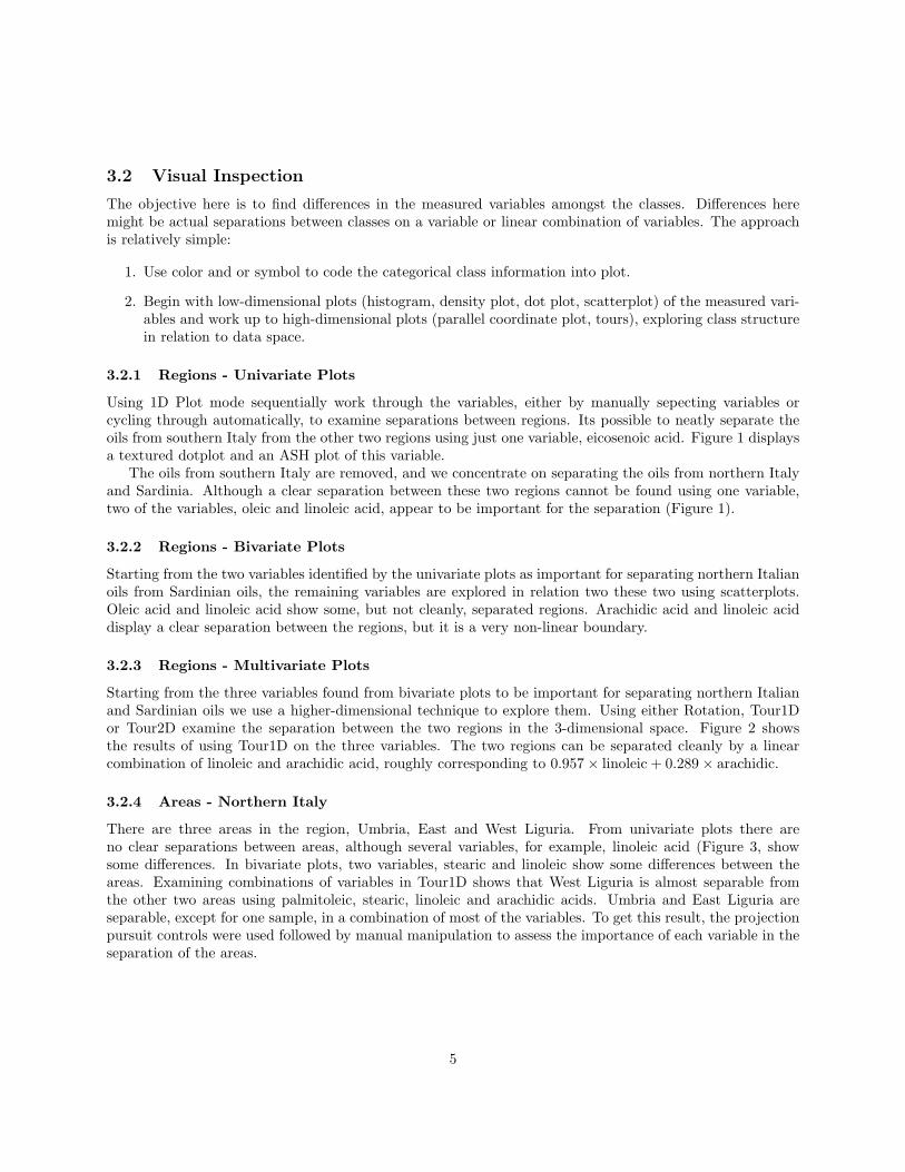
Starting from the two variables identified by the univariate plots as important for separating northern Italianoils from Sardinian oils, the remaining variables are explored in relation two these two using scatterplots.Oleic acid and linoleic acid show some, but not cleanly, separated regions. Arachidic acid and linoleic aciddisplay a clear separation between the regions, but it is a very non-linear boundary.
3.2.3 Regions - Multivariate Plots
Starting from the three variables found from bivariate plots to be important for separating northern Italianand Sardinian oils we use a higher-dimensional technique to explore them. Using either Rotation, Tour1Dor Tour2D examine the separation between the two regions in the 3-dimensional space. Figure 2 showsthe results of using Tour1D on the three variables. The two regions can be separated cleanly by a linearcombination of linoleic and arachidic acid, roughly corresponding to 0.957× linoleic + 0.289× arachidic.
3.2.4 Areas - Northern Italy
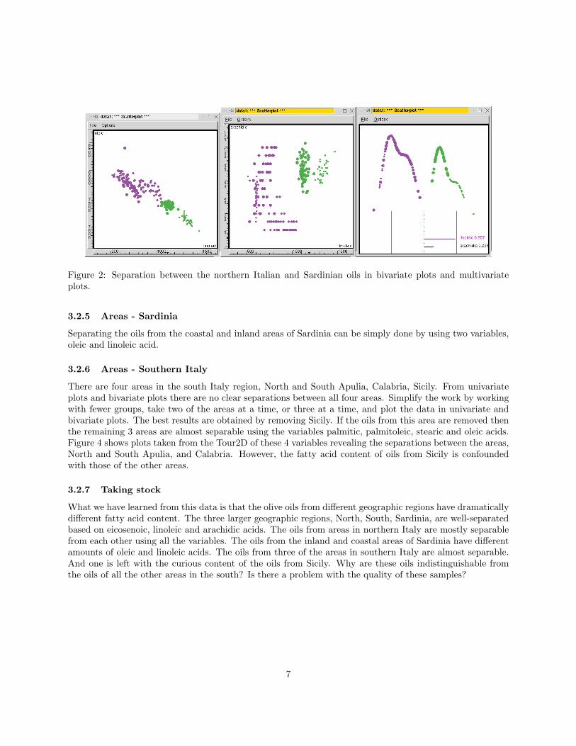
There are three areas in the region, Umbria, East and West Liguria. From univariate plots there areno clear separations between areas, although several variables, for example, linoleic acid (Figure 3, showsome differences. In bivariate plots, two variables, stearic and linoleic show some differences between theareas. Examining combinations of variables in Tour1D shows that West Liguria is almost separable fromthe other two areas using palmitoleic, stearic, linoleic and arachidic acids. Umbria and East Liguria areseparable, except for one sample, in a combination of most of the variables. To get this result, the projectionpursuit controls were used followed by manual manipulation to assess the importance of each variable in theseparation of the areas.
5
Figure 1: Separation between the 3 regions of Italian olive oil data in univariate plots.
6
Figure 2: Separation between the northern Italian and Sardinian oils in bivariate plots and multivariateplots.
3.2.5 Areas - Sardinia
Separating the oils from the coastal and inland areas of Sardinia can be simply done by using two variables,oleic and linoleic acid.
3.2.6 Areas - Southern Italy
There are four areas in the south Italy region, North and South Apulia, Calabria, Sicily. From univariateplots and bivariate plots there are no clear separations between all four areas. Simplify the work by workingwith fewer groups, take two of the areas at a time, or three at a time, and plot the data in univariate andbivariate plots. The best results are obtained by removing Sicily. If the oils from this area are removed thenthe remaining 3 areas are almost separable using the variables palmitic, palmitoleic, stearic and oleic acids.Figure 4 shows plots taken from the Tour2D of these 4 variables revealing the separations between the areas,North and South Apulia, and Calabria. However, the fatty acid content of oils from Sicily is confoundedwith those of the other areas.
3.2.7 Taking stock
What we have learned from this data is that the olive oils from different geographic regions have dramaticallydifferent fatty acid content. The three larger geographic regions, North, South, Sardinia, are well-separatedbased on eicosenoic, linoleic and arachidic acids. The oils from areas in northern Italy are mostly separablefrom each other using all the variables. The oils from the inland and coastal areas of Sardinia have differentamounts of oleic and linoleic acids. The oils from three of the areas in southern Italy are almost separable.And one is left with the curious content of the oils from Sicily. Why are these oils indistinguishable fromthe oils of all the other areas in the south? Is there a problem with the quality of these samples?
7
Figure 3: Separation in the oils from areas of northern Italy, univariate, bivariate and multivariate plots.
8
Figure 4: The areas of southern Italy are mostly separable, except for Sicily.
3.3 Numerical Analysis
The data is broken into training and test samples for this part of the analysis. Approximately 25% of caseswithin each group are reserved for the test samples. These are the cases used for the test sample, where thedata has been sorted by region and area:
Region Area # Train # TestSouth N. Apul. 19 6South Calabria 42 14South S. Apul 158 48South Sicily 27 9Sard Inland 49 16Sard Coast 25 8North E. Lig. 38 12North W. Lig. 38 12North Umbria 40 11
We will use what we learned from the visual analysis to guide the numerical analysis. Some methodsrestrict classification to just two groups, so we will use this restriction with all the classification methods.We will also drop the Sicilian oils from the study - because there is some question raised about the validityof these oils. Here is the binary classification steps we will follow:
9
3.3.1 Methods Used
Classification trees generate a classification tree by sequentially doing binary splits on variables. Splits aredecided on according to the variable and split value which produces the lower measure of impurity. Thereare several common measures of impurity, Gini and deviance. For example, for a two class problem with400 observations in each class, denoted as (400,400), variable 1 produces a split of (300,100) and (100,300),and variable 2 produces a split (200,400) and (200,0). The split on variable 2 will produce a lower impurityvalue because one branch is more pure. There are numerous implementations: R packages such as rpartand standalone packages such as C4.5, C5.0.
Classical Linear discriminant analysis (LDA) assumes that the populations come from multivariate normaldistributions with different mean but equal variance-covariance matrices. Linear boundaries result, and itis possible to reduce the dimension of the data into the space of maximum separation using canonicalcoordinates. The MASS package in R has functions for LDA.
Quadratic discriminant analysis (QDA) assumes that the populations come from multivariate normaldistributions with different mean and different variance-covariance. Non-linear boundaries are the result.The MASS package in R has functions for LDA.
Feed-forward neural networks provide a flexible way to generalize linear regression functions. A simplenetwork model as produced by nnet code in R (Venables & Ripley 1994) may be represented by the equation:
y = φ(α +s∑
h=1
whφ(αh +p∑
i=1
wihxi))
where x is the vector of explanatory variable values, y is the target value, p is the number of variables, s is
10
the number of nodes in the single hidden layer and φ is a fixed function, usually a linear or logistic function.This model has a single hidden layer, and univariate output values.
SVM have recently gained widespread attention due to their success at prediction in classification prob-lems. The subject started in the late seventies (Vapnik 1979). The definitive reference is Vapnik (1999), andBurges (1998) gives a simpler tutorial into the subject. The main difference between this and the previouslydescribed classification techniques is that SVMs really only work for separating between 2 groups. Thereare some modifications for multiple groups but these are little more than one might do manually by workingpairwise through the groups. SVM algorithms work by finding a subset of points in the two groups that canbe separated, which are then known as the support vectors. These support vectors can be used to definea separating hyperplane, w.x + b = 0, where w =
∑NS
i=1 αiyixi, NS is the number of support vectors, andα comes from the constraint
∑NS
i=1 αiyi = 0. Actually we search for the support vectors which gives thehyperplane which gives the biggest separation between the two classes. Note that it is posssible to incorpo-rate non-linear kernel functions allows for defining non-linear separations, and also that modifications allowSVMs to perform well when the classes are not separable. We use the software SVM Light: binary anddocumentation at http://svmlight.joachims.org/
3.3.2 The Classification
Separating RegionsIn separating the southern oils from the other two regions, and then northern oils from Sardinian oils,
here is the classification tree solution:
If eicosenoic acid $>$ 7 then the region is South (1)ElseIf linoleic $>$ 1053.5 then the region is Sardinia (2)Else the region is North (3)
There are no missclassifications on the first split but the second split is problematic. It is a perfectseparation for this data but there is no gap between the two groups. This is easily seen from the plot of thetwo variables used, Figure 5. So at this point we will shift to using a different method to build a classificationrule for northen oils from Sardinian oils.
Here is the R code:
# South vs othersd.olive.train<-d.olive[indx.tr,-c(1,2)]d.olive.test<-d.olive[indx.tst,-c(1,2)]c1<-rep(-1,572)c1[d.olive[,1]!=1]<-1c1.train<-c1[indx.tr]c1.test<-c1[indx.tst]
# North vs Sardiniad.olive.train<-d.olive[indx.tr,]c1.train<-c(rep(-1,572))[indx.tr]c1.train[d.olive.train[,1]==3]<-1c1.train<-c1.train[d.olive.train[,1]!=1]d.olive.train<-d.olive.train[d.olive.train[,1]!=1,-c(1,2)]d.olive.test<-d.olive[indx.tst,]c1.test<-c(rep(-1,572))[indx.tst]
11
Figure 5: (Left)Plot illustrating the results of tree classifier. (Right) Second boundary from LDA solution,dashed boundary is the tree solution on the LDA predicted values.
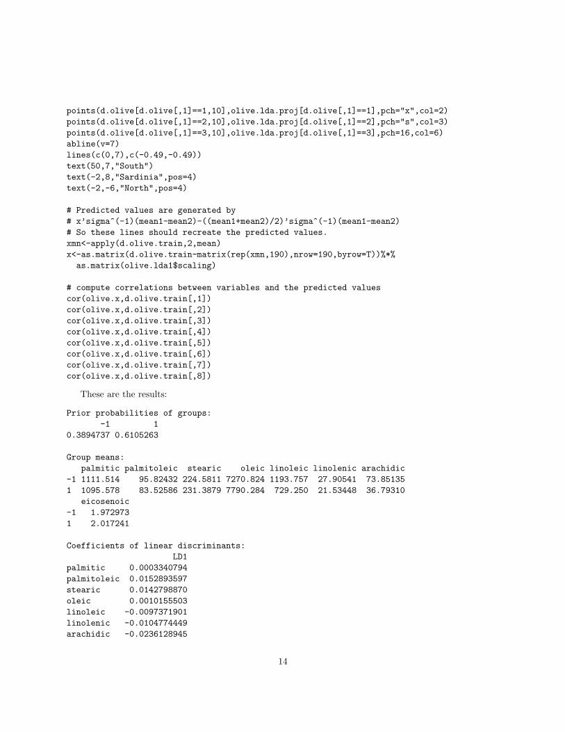
LDA results in errors in the training sample (error rate = 1/190 = 0.005) and no errors in the test sample.The predicted values are well-separated (see figure) but the boundary is in the wrong place! (See Figure 5,right plot.)
Table 1: Correlations between predicted values and the predictors.
The variables oleic, linoleic and arachidic are highly correlated with the predicted values (Table 1). Thepredicted values show a big gap between the northern oils and the sardinian oils but the boundary is set tooclose to the sardinian group because LDA assumes equal variances.
# plot the predictions of the current sampleolive.x<-predict(olive.lda1,d.olive.train, dimen=1)$xolive.x2<-predict(olive.lda1,d.olive.test, dimen=1)$xolive.lda.proj<-predict(olive.lda1,d.olive[,-c(1,2)],dimen=1)$x
# Predicted values are generated by# x’sigma^(-1)(mean1-mean2)-((mean1+mean2)/2)’sigma^(-1)(mean1-mean2)# So these lines should recreate the predicted values.xmn<-apply(d.olive.train,2,mean)x<-as.matrix(d.olive.train-matrix(rep(xmn,190),nrow=190,byrow=T))%*%as.matrix(olive.lda1$scaling)
# compute correlations between variables and the predicted valuescor(olive.x,d.olive.train[,1])cor(olive.x,d.olive.train[,2])cor(olive.x,d.olive.train[,3])cor(olive.x,d.olive.train[,4])cor(olive.x,d.olive.train[,5])cor(olive.x,d.olive.train[,6])cor(olive.x,d.olive.train[,7])cor(olive.x,d.olive.train[,8])
These are the results:
Prior probabilities of groups:-1 1
0.3894737 0.6105263
Group means:palmitic palmitoleic stearic oleic linoleic linolenic arachidic
Quadratic discriminant analysis provides a perfect classification but its more difficult to determine thelocation of the boundary between the two groups.
Trees calculated on the predicted values provide a perfect classification, although the boundary seems alittle too close to the northern oils (Figure 5).
# Check if trees will give a better boundaryrpart(c1.train~olive.x,method="class")par(lty=2)lines(c(0,7),c(-1.49,-1.49))par(lty=1)
This gives the classification of the regions as:
If eicosenoic acid > 7 then the region is South (1)Else
If 0.0003×palmitic +0.0153×palmitoleic +0.01423×stearic +0.0010×oleic −0.0097×linoleic -0.0105×linolenic −0.0236×arachidic −0.1193×eicosenoic - 2.12 > -1.49 then the region is Sardinia (2)
Else the region is North (3)
There is no error associated with this rule.
Sardinian OilsSplit the samples into training and test sets.
Figure 6: Separation of the inland and coastal Sardinian oils using trees (horizontal axis) and LDA (verticalaxis).
A classification tree produces a perfect classification of both training and test samples but the separationbetween groups is rather small relative to the split for a slightly more complex solution provided by LDA(Figure 6). Here is the code:
If 0.0097×palmitic +0.0018×palmitoleic +0.0276×stearic +0.00075×oleic +0.0271×linoleic +0.0750×linolenic−0.0260×arachidic −0.0400×eicosenoic - 55.04 > 0.73 then the sample is from inland Sardinia.
Table 2: Correlations between variables and predicted values for Sardinian oils.
Based on correlations with the predicted values (Table 2) the important variables for separating inland andcoastal Sardinia are oleic, linoleic and stearic acids, with palmitic and linolenic being somewhat important.
Northern OilsSeparating these northern oils is more difficult, based on our visual analysis.
East Liguria vs West Liguria,UmbriaThe classification difficulty is reflected in the results of tree classifiers: the error in the training set is
8/116 = 0.07 and the error in the test set is 8/35 = 0.23. But is is a simple solution using just two variables,palmitic and arachidic. (See Figure 7 left plot.)
The LDA solution is a littler better, with 6/116 = 0.05 errors in the training set and 3/35 = 0.09 in thetest set (Figure 7).
# East Liguria vs others# Treesolive.rp<-rpart(c1.train~.,data.frame(d.olive.train),method="class")olive.rptable(c1.train,predict(olive.rp,type="class"))table(c1.test,predict(olive.rp,data.frame(d.olive.test),type="class"))
# Linear discriminant analysisolive.lda1<-lda(d.olive.train,c1.train)olive.lda1table(c1.train,predict(olive.lda1,d.olive.train)$class)table(c1.test,predict(olive.lda1,d.olive.test)$class)olive.x<-predict(olive.lda1,d.olive.train)$xolive.x2<-predict(olive.lda1,d.olive.test)$x
# compute correlations between variables and the predicted valuescor(olive.x,d.olive.train[,1])cor(olive.x,d.olive.train[,2])cor(olive.x,d.olive.train[,3])cor(olive.x,d.olive.train[,4])cor(olive.x,d.olive.train[,5])cor(olive.x,d.olive.train[,6])cor(olive.x,d.olive.train[,7])cor(olive.x,d.olive.train[,8])
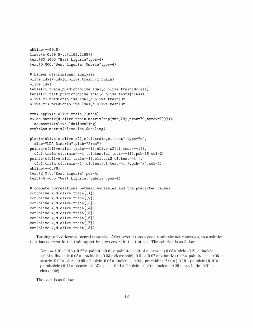
Turning to feed-forward neural networks. After several runs a good result the net converges, to a solutionthat has no error in the training set but two errors in the test set. The solution is as follows:
Figure 7: (Left) Tree solution for East Liguria vs West Liguria,Umbria, (Middle) LDA solution for EastLiguria vs West Liguria,Umbria, (Right) LDA solution for West Liguria vs Umbria.
# weights: 31initial value 101.133439iter 10 value 100.792293iter 20 value 88.353498...iter 560 value 0.004900final value 0.004900converged> table(c1.train,round(predict(olive.nn,d.olive.train)))
Support vector machines (SVM) produce 2 errors in the training set and 6 errors in the test set. TheWindows version of SVM light is used. To run SVM the data needs to be outputted to file in a specialformat. The svm learn and svm classify executables are run in a command window. The parametersneeds to be adjusted some to get the best results. Linear kernels are used.
The neural network solution is the best but not substantially different from the LDA solution in test seterror. So we will use the LDA solution which is a little simpler.
West Liguria vs UmbriaTrees result in no errors in the training set and 2/22 = 0.09 errors in the test set. LDA results in no
errors in either training or test sets (Figure 7).
19
# West Liguria vs Umbriad.olive.train2<-d.olive[indx.tr,]c2.train<-c(rep(-1,572))[indx.tr]c2.train[d.olive.train2[,2]==8]<-1c2.train<-c2.train[d.olive.train2[,1]==3&d.olive.train2[,2]!=7]d.olive.train2<-d.olive.train2[d.olive.train2[,1]==3&d.olive.train2[,2]!=7,-c(1,2)]
If 0.0285×palmitic +0.0009×palmitoleic +0.0317×stearic +0.0187×oleic +0.0180×linoleic −0.0264×linolenic +0.0768×arachidic +0.0795×eicosenoic - 200.0 > 0.76then the sample is from East Liguria
W. Lig vs Umb -0.34 0.80 0.76 -0.88 0.94 -0.93 -0.85 0.05
Table 3: Correlations between variables and predicted values for northern oils.
Based on correlations with the predicted values (Table 3) the important variables for separating EastLiguria are palmitic and arachidic, and for separating West Liguria from Umbria the important variablesare palmitoleic, stearic, oleic, linoleic, linolenic, arachidic.
Southern Oils
The areas of the southern region promised to be the most difficult to classify. We ignore Sicily to begin.Calabria vs Others
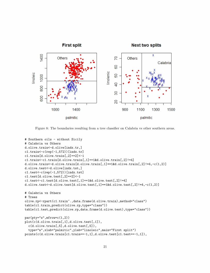
With trees there are 4/219 = 0.018 errors in the training set, and 2/68 = 0.029 errors in the test set. Theplots in Figure 8 illustrate the splits. This is about the best solution of all the methods, surprisingly! Thereare too many errors in the training set, but the most important error to guard against is the test error, andtrees give the smallest test error. LDA results in 4/219 = 0.18 errors in the training set and 5/68 = 074errors in the test set. QDA results in only 1/219 = 0.004 in the training set but 3/68 = 0.044 in the testset. The best results for FFNN were 0 errors in the training set but 3/68− 0.044 errors in the test set. SVMhad 1 error in the training set and 4 errors in the test set.
This is the code:
20
Figure 8: The boundaries resulting from a tree classifier on Calabria vs other southern areas.
# Southern oils - without Sicily# Calabria vs Othersd.olive.train<-d.olive[indx.tr,]c1.train<-c(rep(-1,572))[indx.tr]c1.train[d.olive.train[,2]==2]<-1c1.train<-c1.train[d.olive.train[,1]==1&d.olive.train[,2]!=4]d.olive.train<-d.olive.train[d.olive.train[,1]==1&d.olive.train[,2]!=4,-c(1,2)]d.olive.test<-d.olive[indx.tst,]c1.test<-c(rep(-1,572))[indx.tst]c1.test[d.olive.test[,2]==2]<-1c1.test<-c1.test[d.olive.test[,1]==1&d.olive.test[,2]!=4]d.olive.test<-d.olive.test[d.olive.test[,1]==1&d.olive.test[,2]!=4,-c(1,2)]
# Calabria vs Others# Treesolive.rp<-rpart(c1.train~.,data.frame(d.olive.train),method="class")table(c1.train,predict(olive.rp,type="class"))table(c1.test,predict(olive.rp,data.frame(d.olive.test),type="class"))
plot(c(d.olive.train[d.olive.train[,5]<946,1],d.olive.test[d.olive.test[,5]<946,1]),c(d.olive.train[d.olive.train[,5]<946,6],d.olive.test[d.olive.test[,5]<946,6]),type="n",xlab="palmitic",ylab="linolenic",main="Next two splits")
# Linear discriminant analysisolive.lda1<-lda(d.olive.train,c1.train)olive.lda1table(c1.train,predict(olive.lda1,d.olive.train)$class)table(c1.test,predict(olive.lda1,d.olive.test)$class)olive.x<-predict(olive.lda1,d.olive.train)$xolive.x2<-predict(olive.lda1,d.olive.test)$x
# FFNN# weights: 51initial value 144.303546iter 10 value 69.334956.....iter 250 value 0.542601final value 0.542600converged
c1.train -1 1-1 177 01 0 42
c1.test -1 0 1-1 53 0 11 1 1 12
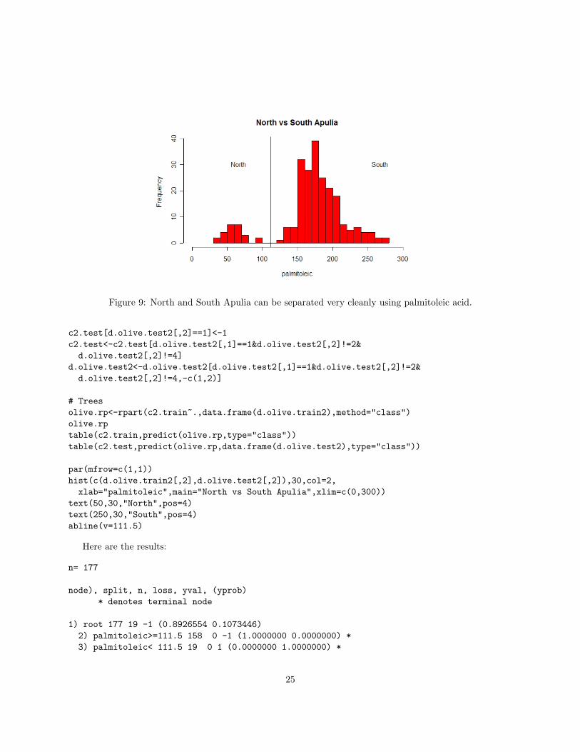
North vs South ApuliaThese two areas turn out to be very easy to separate, using trees. The training and test sets are both
perfectly classified using palmitoleic acid (Figure 9).Here is the code:
# North Apulia vs South Apuliad.olive.train2<-d.olive[indx.tr,]c2.train<-c(rep(-1,572))[indx.tr]c2.train[d.olive.train2[,2]==1]<-1c2.train<-c2.train[d.olive.train2[,1]==1&d.olive.train2[,2]!=2&d.olive.train2[,2]!=4]
Thus the solution for the areas of the southern region (without Sicily) is:
If linoleic>=946If palmitoleic >= 111.5 then the area is South ApuliaElse the area is North Apulia
Else (linoleic<946)If palmitic<1116If palmitoleic >= 111.5 then the area is South Apulia
26
Else the area is North ApuliaElse (palmitic>=1116)If linolenic<37If palmitoleic >= 111.5 then the area is South ApuliaElse the area is North Apulia
Else (linolenic>37) the area is Calabria
The test error associated with this classification is 3%.
27
4 Summary
The classification rule (with values given in % ×100) is then:
If eicosenoic acid > 7 then the region is SouthIf eicosenoic acid < 34.5 then the area is SicilyElse
If stearic < 261If arachidic < 84.5 the area is Sicily
If stearic ≥ 261 OR if (stearic < 261 and arachidic ≥ 84.5)If linoleic ≥ 946
If palmitoleic ≥ 111.5 the area is South ApuliaElse the area is North Apulia
Else (linoleic <946)If palmitic ≥ 1116
If palmitoleic ≥ 111.5 the area is South ApuliaElse the area is North Apulia
Else (palmitic ≥ 1116)If linolenic < 37
If palmitoleic ≥ 111.5 then the area is South ApuliaElse the area is North Apulia
Else (linolenic > 37) the area is CalabriaElse
If 0.0003×palmitic +0.0153×palmitoleic +0.01423×stearic +0.0010×oleic −0.0097×linoleic -0.0105×linolenic −0.0236×arachidic −0.1193×eicosenoic - 2.12 > -1.49 then the region is SardiniaIf 0.0097×palmitic +0.0018×palmitoleic +0.0276×stearic +0.00075×oleic +0.0271×linoleic+
0.0750×linolenic −0.0260×arachidic −0.0400×eicosenoic - 55.04 > 0.73 then the sample isfrom inland Sardinia
Else the sample is from coastal SardiniaElse the region is North
If 0.0285×palmitic +0.0009×palmitoleic +0.0317×stearic +0.0187×oleic +0.0180×linoleic −0.0264×linolenic +0.0768×arachidic +0.0795×eicosenoic - 200.0 > 0.76then the sample is from East Liguria
0.0172×linoleic −0.0627×linolenic −0.0342×arachidic −0.2244×eicosenoic - 128.0 > -0.03then the sample is from West Liguria
Else it is from Umbria
The error on the test set overall is (3 + 7 + 2)/136 = 0.09 including Sicily and 5/127 = 0.04 withoutSicily, and separately on the areas is given in Table 4. The important variables in each of the separationsare given in Table 5.
There are several qualifications about the study:
• We are assuming that the data samples have been collected appropriately, that the samples are repre-sentative of the oils of the areas they are purported to be produced in.
• There is a big difference in the sample sizes for each class. South Apulia is the most abundantlyrepresented and form the internet search of material this is one of the most prolific olive oil producing
28
Classes Test ErrorOverall (with Sicily) 12/136=0.09Overall (without Sicily) 5/127=0.04South vs Others 0/136 =0North vs Sardinia 0/59 =0Inland vs Coastal Sardinia 0/24=0East Liguria vs Others 3/35=0.09Umbria vs West Liguria 0/23=0Sicily vs Others 7/77=0.09Calabria vs Others 2/68=0.03North vs South Apulia 0/54=0
Table 5: This table marks the important variables for each separation.
areas. North Apulia has the least samples, only 25. Perhaps the sample size is indicative of theproductivity and should perhaps be incorporated into the classifiers.
29
References
Burges, C. J. C. (1998), ‘A Tutorial Support Vector Machines for Pattern Recognition’, Data Mining andKnowledge Discovery 2, 121–167.
Forina, M., Armanino, C., Lanteri, S. & Tiscornia, E. (1983), Classification of olive oils from their fattyacid composition, in H. Martens & H. Russwurm Jr., eds, ‘Food Research and Data Analysis’, AppliedScience Publishers, London, pp. 189–214.
Vapnik, V. (1979), Estimation of Dependence Based on Empirical Data (In Russian), Nauka, Moscow.
Vapnik, V. (1999), The Nature of Statistical Learning Theory (Statistics for Engineering and InformationScience), Springer-Verlag, New York, NY.
Venables, W. N. & Ripley, B. (1994), Modern Applied Statistics with S-Plus, Springer-Verlag, New York.


![Wheat/Dairy/Corn-free Ingredients & Foods...• Light Coconut Milk • Extra Virgin Olive Oil (any of Trader Joe's olive oils, organic or not) [no image] 5 OILS, SAUCES, CONDIMENTS,](https://static.documents.pub/doc/80x56/5f6a5e6c87a61a68241363ed/wheatdairycorn-free-ingredients-foods-a-light-coconut-milk-a-extra.jpg)


