1 Electronic Supplemental Material for the study "Are Measuring Concern About the Global Climate Change Correctly? Testing a Novel Measurement Approach with the Data from 28 Countries" Appendix 1: Socio-demographic characteristics of national samples (rel. frequencies, means, and counts). Country Proporti on of males [%] Avr. age Proportion of people with university or college education [%] 1 Sampl e size Austria 47.4 47.7 22.5 1019 Belgium 48.5 49.6 49.1 1077 Bulgaria 46.7 49.6 34.5 1026 Croatia 44.3 42.9 35.3 1002 Cyprus (Republic) 46.8 49.3 36.6 500 Czech Republic 42.1 46.0 23.5 1018 Denmark 48.6 54.9 80.3 1010 Estonia 40.7 50.3 49.7 1012 Finland 45 55.0 61.6 971 France 46.3 50.5 42.3 1022 Germany 49.5 51.0 33.6 1600 Greece 48.6 47.3 39.2 1007 Hungary 41.5 48.4 21.1 1012 Ireland 44 47.0 36.3 1007 Italy 44 46.9 28.2 1019 Latvia 45.5 43.2 43.6 1011 Lithuania 45.4 46.3 47.8 1023 Luxembourg 40.6 51.1 49.6 510 Malta 40.6 55.1 18.6 500 Netherlands 45.5 52.3 56.8 1037 Poland 38.8 48.2 39.2 1000 Portugal 44.6 51.2 23.1 1055 Romania 50.5 48.9 34.1 1013 Slovakia 42.8 46.1 28.6 1000 Slovenia 41.7 50.7 38.3 1113 Spain 46.9 47.2 32.1 1013 Sweden 50.6 57.1 70.8 1011 United Kingdom 46.5 52.0 28.8 1331
Transcript
1
Electronic Supplemental Material for the study "Are Measuring Concern About the Global Climate Change Correctly? Testing a Novel Measurement Approach with the Data from 28 Countries"
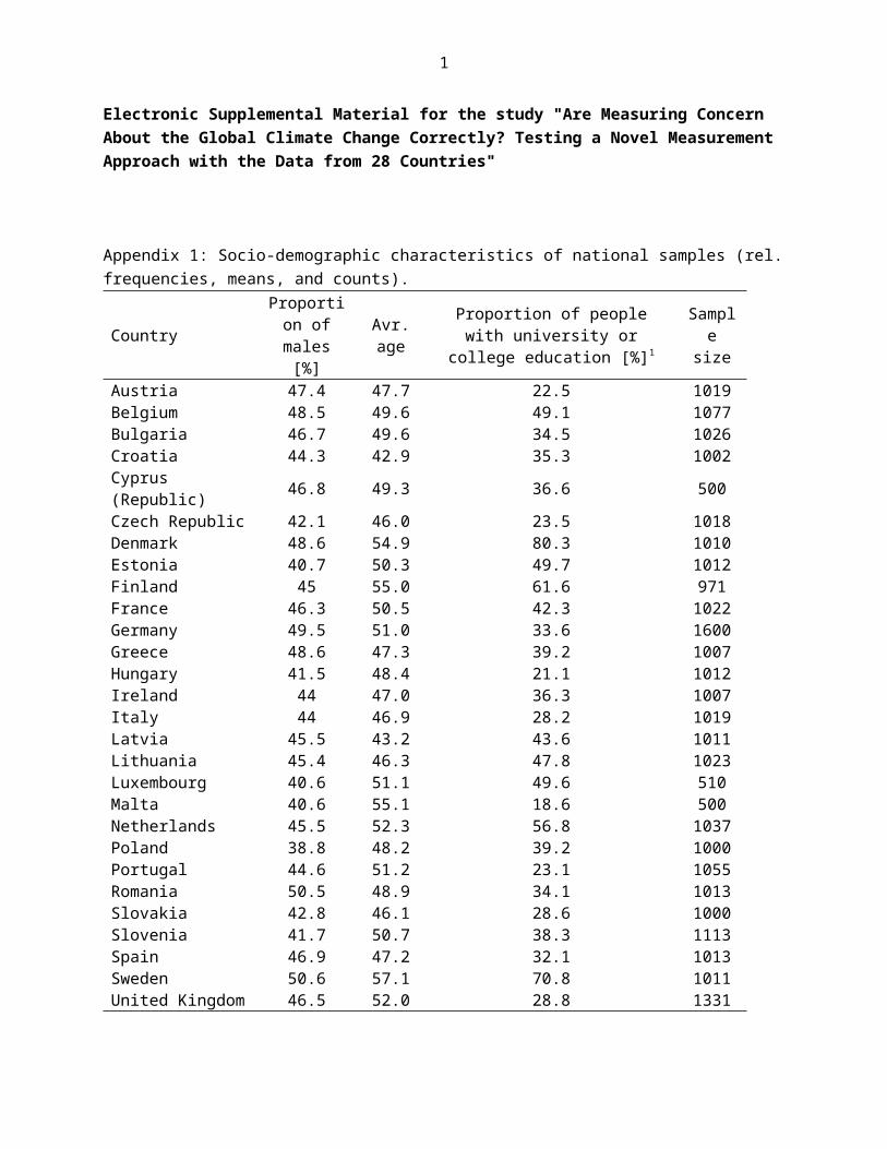
Appendix 1: Socio-demographic characteristics of national samples (rel. frequencies, means, and counts).
Country Proportion of males [%]
Avr. age
Proportion of people with university or college education [%]1
Note: 1 People who finished their full-time studies education at age of 20 or at higher age.
2
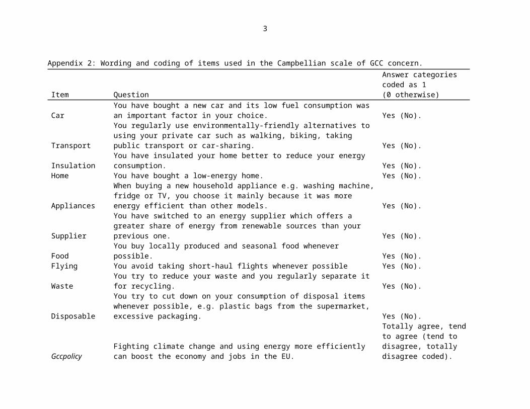
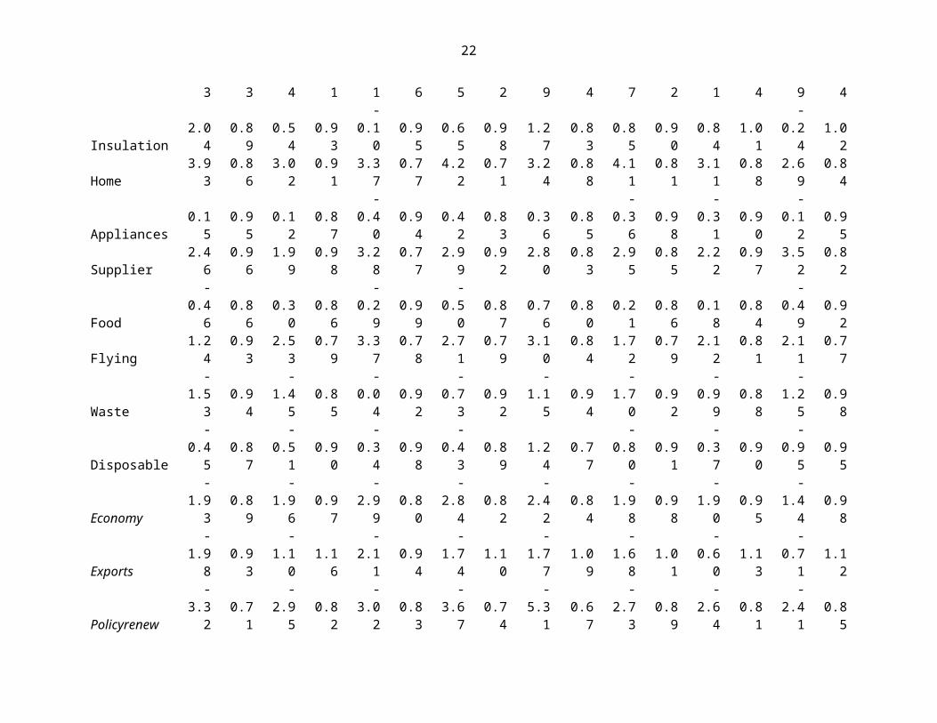
Appendix 2: Wording and coding of items used in the Campbellian scale of GCC concern.
Item QuestionAnswer categories coded as 1 (0 otherwise)
CarYou have bought a new car and its low fuel consumption was an important factor in your choice. Yes (No).
TransportYou regularly use environmentally-friendly alternatives to using your private car such as walking, biking, taking public transport or car-sharing. Yes (No).
Insulation You have insulated your home better to reduce your energy consumption. Yes (No).Home You have bought a low-energy home. Yes (No).
AppliancesWhen buying a new household appliance e.g. washing machine, fridge or TV, you choose it mainly because it was more energy efficient than other models. Yes (No).
SupplierYou have switched to an energy supplier which offers a greater share of energy from renewable sources than your previous one. Yes (No).
Food You buy locally produced and seasonal food whenever possible. Yes (No).Flying You avoid taking short-haul flights whenever possible Yes (No).Waste You try to reduce your waste and you regularly separate it for recycling. Yes (No).
DisposableYou try to cut down on your consumption of disposal items whenever possible, e.g. plastic bags from the supermarket, excessive packaging. Yes (No).
GccpolicyFighting climate change and using energy more efficiently can boost the economy and jobs in the EU.
Totally agree, tend to agree (tend to disagree, totally disagree coded).
Fossilpolicy Reducing fossil fuel imports from outside the EU could benefit the EU economically.
Totally agree, tend to agree (tend to disagree, totally disagree coded).
Renewpolicy
How important do you think it is that the our [nationality specified for each national sample] government sets targets to increase the amount of renewable energy used, such as wind or solar power, by 2030? (1=very important; 2=fairly important; 3=not very important; 4=not at all important)
Very important, fairly important (not very important, not important at all).
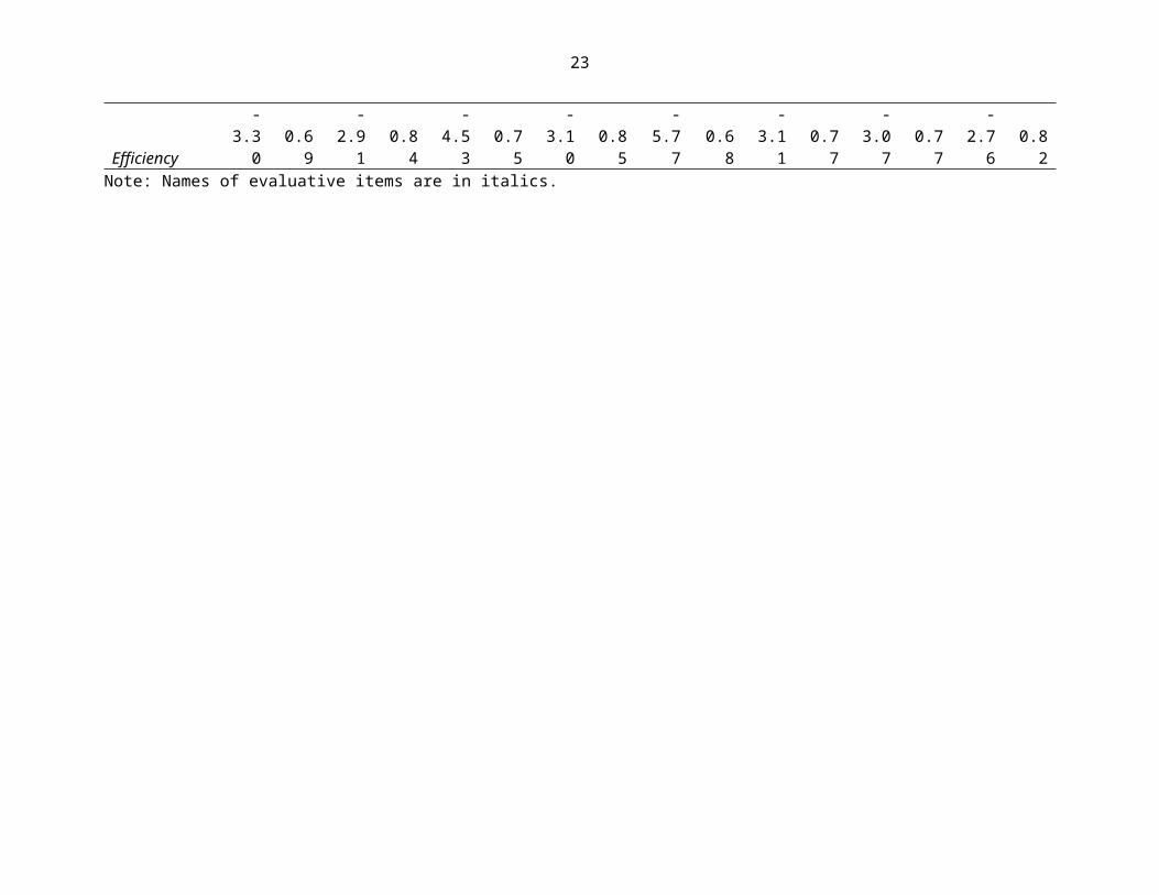
Efficpolicy
How important do you think it is that the our [nationality specified for each national sample] government provides support for improving energy efficiency (for example, by encouraging people to insulate their home or purchase low energy light bulbs) by 2030?
Very important, fairly important (not very important, not important at all).
Note: Names of evaluative items are in italics.
3
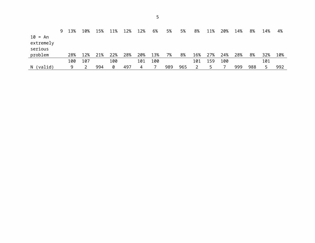
Appendix 3: Country-specific evaluative rating of GCC concern (rel. probabilities).
Concern rating AT BE BG HR CY CZ DK EE FI FR DE GR HU IE IT LV1 = Not at all a serious problem 0% 1% 0% 2% 2% 1% 2% 8% 3% 1% 1% 1% 1% 2% 0% 5%
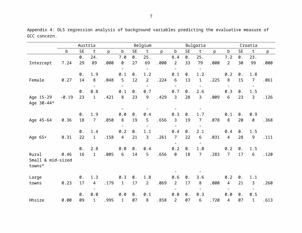
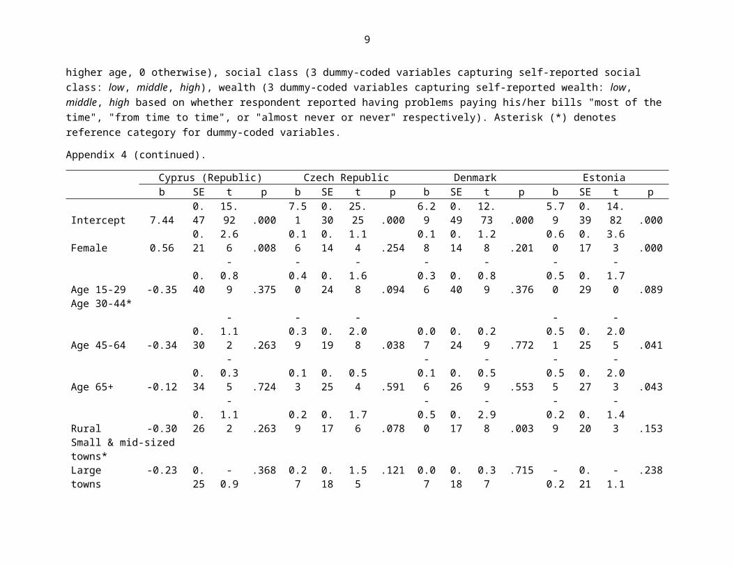
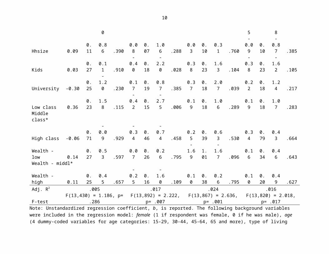
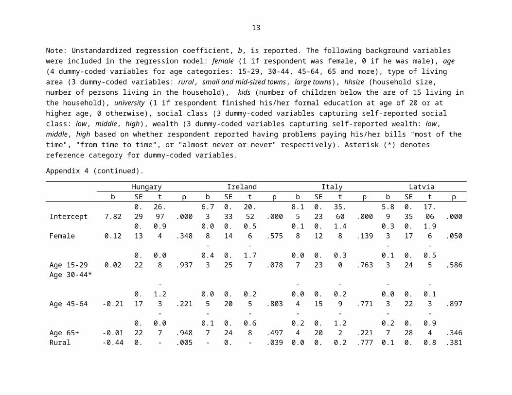
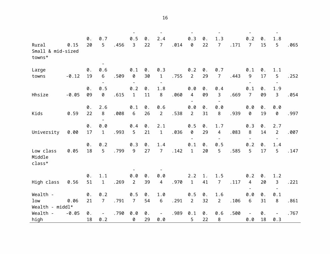
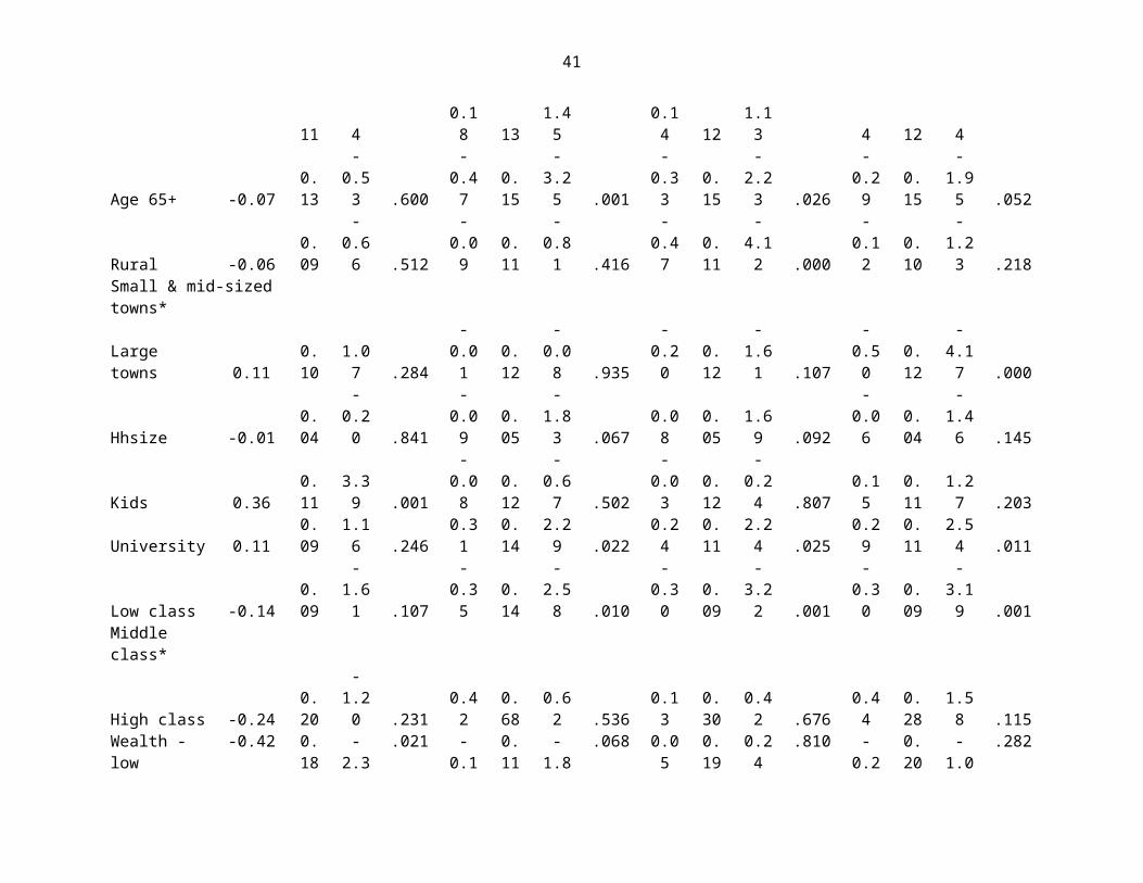
Note: Unstandardized regression coefficient, b, is reported. The following background variables were included in the regression model: female (1 if respondent was female, 0 if he was male), age (4 dummy-coded variables for age categories: 15-29, 30-44, 45-64, 65 and more), type of living area (3 dummy-coded variables: rural, small and mid-sized towns, large towns), hhsize (household size, number of persons living in the household), kids (number of children below the are of 15 living in the household), university (1 if respondent finished his/her formal education at age of 20 or at higher age, 0 otherwise), social class (3 dummy-coded variables capturing self-reported social class: low, middle, high), wealth (3 dummy-coded variables capturing self-reported wealth: low, middle, high based on whether respondent reported having problems paying his/her bills "most of the time", "from time to time", or "almost never or never" respectively). Asterisk (*) denotes reference category for dummy-coded variables.
Note: Unstandardized regression coefficient, b, is reported. The following background variables were included in the regression model: female (1 if respondent was female, 0 if he was male), age (4 dummy-coded variables for age categories: 15-29, 30-44, 45-64, 65 and more), type of living area (3 dummy-coded variables: rural, small and mid-sized towns, large towns), hhsize (household size, number of persons living in the household), kids (number of children below the are of 15 living in the household), university (1 if respondent finished his/her formal education at age of 20 or at higher age, 0 otherwise), social class (3 dummy-coded variables capturing self-reported social class: low, middle, high), wealth (3 dummy-coded variables capturing self-reported wealth: low, middle, high based on whether respondent reported having problems paying his/her bills "most of the time", "from time to time", or "almost never or never" respectively). Asterisk (*) denotes reference category for dummy-coded variables.
Note: Unstandardized regression coefficient, b, is reported. The following background variables were included in the regression model: female (1 if respondent was female, 0 if he was male), age (4 dummy-coded variables for age categories: 15-29, 30-44, 45-64, 65 and more), type of living area (3 dummy-coded variables: rural, small and mid-sized towns, large towns), hhsize (household size, number of persons living in the household), kids (number of children below the are of 15 living in the household), university (1 if respondent finished his/her formal education at age of 20 or at higher age, 0 otherwise), social class (3 dummy-coded variables capturing self-reported social class: low, middle, high), wealth (3 dummy-coded variables capturing self-reported wealth: low, middle, high based on whether respondent reported having problems paying his/her bills "most of the time", "from time to time", or "almost never or never" respectively). Asterisk (*) denotes reference category for dummy-coded variables.
Note: Unstandardized regression coefficient, b, is reported. The following background variables were included in the regression model: female (1 if respondent was female, 0 if he was male), age (4 dummy-coded variables for age categories: 15-29, 30-44, 45-64, 65 and more), type of living area (3 dummy-coded variables: rural, small and mid-sized towns, large towns), hhsize (household size, number of persons living in the household), kids (number of children below the are of 15 living in the household), university (1 if respondent finished his/her formal education at age of 20 or at higher age, 0 otherwise), social class (3 dummy-coded variables capturing self-reported social class: low, middle, high), wealth (3 dummy-coded variables capturing self-reported wealth: low, middle, high based on whether respondent reported having problems paying his/her bills "most of the time", "from time to time", or "almost never or never" respectively). Asterisk (*) denotes reference category for dummy-coded variables.
Note: Unstandardized regression coefficient, b, is reported. The following background variables were included in the regression model: female (1 if respondent was female, 0 if he was male), age (4 dummy-coded variables for age categories: 15-29, 30-44, 45-64, 65 and more), type of living area (3 dummy-coded variables: rural, small and mid-sized towns, large towns), hhsize (household size, number of persons living in the household), kids (number of children below the are of 15 living in the household), university (1 if respondent finished his/her formal education at age of 20 or at higher age, 0 otherwise), social class (3 dummy-coded variables capturing self-reported social class: low, middle, high), wealth (3 dummy-coded variables capturing self-reported wealth: low, middle, high based on whether respondent reported having problems paying his/her bills "most of the time", "from time to time", or "almost never or never" respectively). Asterisk (*) denotes reference category for dummy-coded variables.
Note: Unstandardized regression coefficient, b, is reported. The following background variables were included in the regression model: female (1 if respondent was female, 0 if he was male), age (4 dummy-coded variables for age categories: 15-29, 30-44, 45-64, 65 and more), type of living area (3 dummy-coded variables: rural, small and mid-sized towns, large towns), hhsize (household size, number of persons living in the household), kids (number of children below the are of 15 living in the household), university (1 if respondent finished his/her formal education at age of 20 or at higher age, 0 otherwise), social class (3 dummy-coded variables capturing self-reported social class: low, middle, high), wealth (3 dummy-coded variables capturing self-reported wealth: low, middle, high based on whether respondent reported having problems paying his/her bills "most of the time", "from time to time", or "almost never or never" respectively). Asterisk (*) denotes reference category for dummy-coded variables.
Note: Unstandardized regression coefficient, b, is reported. The following background variables were included in the regression model: female (1 if respondent was female, 0 if he was male), age (4 dummy-coded variables for age categories: 15-29, 30-44, 45-64, 65 and more), type of living area (3 dummy-coded variables: rural, small and mid-sized towns, large towns), hhsize (household size, number of persons living in the household), kids (number of children below the are of 15 living in the household), university (1 if respondent finished his/her formal education at age of 20 or at higher age, 0 otherwise), social class (3 dummy-coded variables capturing self-reported social class: low, middle, high), wealth (3 dummy-coded variables capturing self-reported wealth: low, middle, high based on whether respondent reported having problems paying his/her bills "most of the time", "from time to time", or "almost never or never" respectively). Asterisk (*) denotes reference category for dummy-coded variables.
12
Appendix 5: Difficulty and fit estimates for items forming the Campbellian GCC concern measure (binary Rasch model).
Note: Unstandardized regression coefficient, b, is reported. The following background variables were included in the regression model: female (1 if respondent was female, 0 if he was male), age (4 dummy-coded variables for age categories: 15-29, 30-44, 45-64, 65 and more), type of living area (3 dummy-coded variables: rural, small and mid-sized towns, large towns), hhsize (household size, number of persons living in the household), kids (number of children below the are of 15 living in the household), university (1 if respondent finished his/her formal education at age of 20 or at higher age, 0 otherwise), social class (3 dummy-coded variables capturing self-reported social class: low, middle, high), wealth (3 dummy-coded variables capturing self-reported wealth: low, middle, high based on whether respondent reported having problems paying his/her bills "most of the time", "from time to time", or "almost never or never" respectively). Asterisk (*) denotes reference category for dummy-coded variables.
Note: Unstandardized regression coefficient, b, is reported. The following background variables were included in the regression model: female (1 if respondent was female, 0 if he was male), age (4 dummy-coded variables for age categories: 15-29, 30-44, 45-64, 65 and more), type of living area (3 dummy-coded variables: rural, small and mid-sized towns, large towns), hhsize (household size, number of persons living in the household), kids (number of children below the are of 15 living in the household), university (1 if respondent finished his/her formal education at age of 20 or at higher age, 0 otherwise), social class (3 dummy-coded variables capturing self-reported social class: low, middle, high), wealth (3 dummy-coded variables capturing self-reported wealth: low, middle, high based on whether respondent reported having problems paying his/her bills "most of the time", "from time to time", or "almost never or never" respectively). Asterisk (*) denotes reference category for dummy-coded variables.
Note: Unstandardized regression coefficient, b, is reported. The following background variables were included in the regression model: female (1 if respondent was female, 0 if he was male), age (4 dummy-coded variables for age categories: 15-29, 30-44, 45-64, 65 and more), type of living area (3 dummy-coded variables: rural, small and mid-sized towns, large towns), hhsize (household size, number of persons living in the household), kids (number of children below the are of 15 living in the household), university (1 if respondent finished his/her formal education at age of 20 or at higher age, 0 otherwise), social class (3 dummy-coded variables capturing self-reported social class: low, middle, high), wealth (3 dummy-coded variables capturing self-reported wealth: low, middle, high based on whether respondent reported having problems paying his/her bills "most of the time", "from time to time", or "almost never or never" respectively). Asterisk (*) denotes reference category for dummy-coded variables.
Note: Unstandardized regression coefficient, b, is reported. The following background variables were included in the regression model: female (1 if respondent was female, 0 if he was male), age (4 dummy-coded variables for age categories: 15-29, 30-44, 45-64, 65 and more), type of living area (3 dummy-coded variables: rural, small and mid-sized towns, large towns), hhsize (household size, number of persons living in the household), kids (number of children below the are of 15 living in the household), university (1 if respondent finished his/her formal education at age of 20 or at higher age, 0 otherwise), social class (3 dummy-coded variables capturing self-reported social class: low, middle, high), wealth (3 dummy-coded variables capturing self-reported wealth: low, middle, high based on whether respondent reported having problems paying his/her bills "most of the time", "from time to time", or "almost never or never" respectively). Asterisk (*) denotes reference category for dummy-coded variables.
Note: Unstandardized regression coefficient, b, is reported. The following background variables were included in the regression model: female (1 if respondent was female, 0 if he was male), age (4 dummy-coded variables for age categories: 15-29, 30-44, 45-64, 65 and more), type of living area (3 dummy-coded variables: rural, small and mid-sized towns, large towns), hhsize (household size, number of persons living in the household), kids (number of children below the are of 15 living in the household), university (1 if respondent finished his/her formal education at age of 20 or at higher age, 0 otherwise), social class (3 dummy-coded variables capturing self-reported social class: low, middle, high), wealth (3 dummy-coded variables capturing self-reported wealth: low, middle, high based on whether respondent reported having problems paying his/her bills "most of the time", "from time to time", or "almost never or never" respectively). Asterisk (*) denotes reference category for dummy-coded variables.
21
Appendix 6 (continued).
Poland Portugal Romania Slovakia b SE t p b SE t p b SE t p b SE t p
2Adj. R2 .033 .037 .073 .067F-test F(13,816) = 3.208, p < .001 F(13,849) = 3.53, p < .001 F(13,854) = 6.261, p < .001 F(13,832) = 5.632, p < .001
Note: Unstandardized regression coefficient, b, is reported. The following background variables were included in the regression model: female (1 if respondent was female, 0 if he was male), age (4 dummy-coded variables for age categories: 15-29, 30-44, 45-64, 65 and more), type of living area (3 dummy-coded variables: rural, small and mid-sized towns, large towns), hhsize (household size, number of persons living in the household), kids (number of children below the are of 15 living in the household), university (1 if respondent finished his/her formal education at age of 20 or at higher age, 0 otherwise), social class (3 dummy-coded variables capturing self-reported social class: low, middle, high), wealth (3 dummy-coded variables capturing self-reported wealth: low, middle, high based on whether respondent reported having problems paying his/her bills "most of the time", "from time to time", or "almost never or never" respectively). Asterisk (*) denotes reference category for dummy-coded variables.
Wealth - high 0.34 0.09 3.85 .000 0.31 0.11 2.84 .005 0.18 0.18 1.01 .313 -0.13 0.11 -1.23 .220Adj. R2 .081 .084 .053 .075F-test F(13,925) = 7.398, p < .001 F(13,872) = 7.277, p < .001 F(13,911) = 5.006, p < .001 F(13,1135) = 8.112, p < .001
Note: Unstandardized regression coefficient, b, is reported. The following background variables were included in the regression model: female (1 if respondent was female, 0 if he was male), age (4 dummy-coded variables for age categories: 15-29, 30-44, 45-64, 65 and more), type of living area (3 dummy-coded variables: rural, small and mid-sized towns, large towns), hhsize (household size, number of persons living in the household), kids (number of children below the are of 15 living in the household), university (1 if respondent finished his/her formal education at age of 20 or at higher age, 0 otherwise), social class (3 dummy-coded variables capturing self-reported social class: low, middle, high), wealth (3 dummy-coded variables capturing self-reported wealth: low, middle, high based on whether respondent reported having problems paying his/her bills "most of the time", "from time to time", or "almost never or never" respectively). Asterisk (*) denotes reference category for dummy-coded variables.
24
Appendix 7: Results of ANCOVA test of effects of background variables and criterion variable (installation of renewables) on the Campbellian measure of GCC concern.
Austria Belgium Bulgaria Croatia
Df SS MSS F p η2 Df SS MSS F p η2 Df SS MSS F p η2 Df SS MSS F p η2
Gender 1 20.78 20.78 14.50 .000 .016 1 0.16 0.16 0.12 .726 .000 1 0.01 0.01 0.01 .936 .000 1 4.97 4.97 4.00 .046 .002Age 3 22.28 7.43 5.18 .001 .019 3 16.60 5.54 4.19 .006 .009 3 51.76 17.25 11.84 .000 .024 3 16.23 5.41 4.36 .005 .016Area 2 15.11 7.56 5.27 .005 .014 2 15.36 7.68 5.82 .003 .011 2 36.35 18.18 12.48 .000 .017 2 1.91 0.96 0.77 .464 .001Hhsize 1 14.32 14.32 10.00 .002 .008 1 3.45 3.45 2.62 .106 .001 1 0.77 0.77 0.53 .468 .001 1 0.53 0.53 0.43 .515 .000Kids 1 1.41 1.41 0.98 .322 .001 1 2.07 2.07 1.57 .211 .002 1 6.20 6.20 4.26 .039 .003 1 3.70 3.70 2.98 .085 .004University 1 12.58 12.58 8.78 .003 .007 1 49.11 49.11 37.21 .000 .018 1 33.76 33.76 23.17 .000 .017 1 9.65 9.65 7.77 .005 .008Class 2 2.98 1.49 1.04 .354 .002 2 21.88 10.94 8.29 .000 .011 2 2.73 1.36 0.94 .393 .002 2 10.11 5.06 4.07 .017 .008Wealth 2 0.33 0.16 0.11 .892 .000 2 21.19 10.60 8.03 .000 .016 2 2.90 1.45 1.00 .370 .002 2 4.41 2.21 1.78 .170 .004Renewables 1 3.68 3.68 2.57 .110 .003 1 6.86 6.86 5.20 .023 .006 1 7.57 7.57 5.20 .023 .007 1 4.97 4.97 4.00 .046 .005Residuals 809 1159 1.43 948 1251 1.32 788 1148 1.46 812 1009 1.24Sample size 1010 1073 987 996 Note: The following background variables were included in the regression model: gender (0 if respondent was male, 1 if she was female), age (4 age categories: 15-29, 30-44, 45-64, 65 and more), area (3 categories of living area: rural, small and mid-sized towns, large towns), hhsize (household size, number of persons living in the hoousehold), kids (number of children below the are of 15 living in the household), university (1 if respondent finished his/her formal education at age of 20 or at higher age, and 0 otherwise), class (3 categories of self-reported social class: low, middle, high), wealth (3 categories of self-reported wealth: low, middle, high based on whether respondent reported having problems paying his/her bills "most of the time", "from time to time", or "almost never or never"), renewables (criterion test variable, 1 if respondent has installed renewables, 0 otherwise).
25
Appendix 7 (continued).
Cyprus (Republic) Czech Republic Denmark Estonia
Df SS MSS F p η2 Df SS MSS F p η2 Df SS MSS F p η2 Df SS MSS F p η2
Gender 1 0.00 0.00 0.00 .985 .000 1 3.96 3.96 3.62 .058 .006 1 21.07 21.07 19.41 .000 .020 1 17.33 17.33 15.35 .000 .018Age 3 44.31 14.77 6.91 .000 .050 3 16.83 5.61 5.12 .002 .017 3 7.22 2.41 2.22 .085 .001 3 14.83 4.95 4.38 .005 .004Area 2 16.44 8.22 3.84 .022 .007 2 17.79 8.89 8.12 .000 .016 2 3.12 1.56 1.44 .238 .002 2 4.41 2.21 1.95 .142 .002Hhsize 1 0.29 0.29 0.14 .714 .000 1 4.68 4.68 4.28 .039 .003 1 21.62 21.62 19.91 .000 .013 1 4.57 4.57 4.05 .044 .004Kids 1 1.16 1.16 0.54 .462 .001 1 1.91 1.91 1.74 .187 .002 1 1.72 1.72 1.59 .208 .001 1 0.81 0.81 0.72 .397 .001University 1 23.26 23.26 10.88 .001 .003 1 1.09 1.09 1.00 .318 .000 1 12.62 12.62 11.62 .001 .008 1 5.75 5.75 5.09 .024 .002Class 2 42.97 21.49 10.05 .000 .020 2 3.12 1.56 1.42 .241 .002 2 17.59 8.80 8.10 .000 .016 2 7.28 3.64 3.22 .040 .005Wealth 2 34.82 17.41 8.14 .000 .034 2 4.04 2.02 1.85 .159 .004 2 2.64 1.32 1.21 .297 .003 2 2.76 1.38 1.22 .295 .003Renewables 1 3.80 3.80 1.78 .183 .004 1 0.94 0.94 0.86 .354 .001 1 2.08 2.08 1.92 .166 .002 1 0.66 0.66 0.59 .444 .001Residuals 432 924 2.14 892 977 1.10 869 944 1.09 836 944 1.13 Sample size 499 1009 1009 992Note: The following background variables were included in the regression model: gender (0 if respondent was male, 1 if she was female), age (4 age categories: 15-29, 30-44, 45-64, 65 and more), area (3 categories of living area: rural, small and mid-sized towns, large towns), hhsize (household size, number of persons living in the hoousehold), kids (number of children below the are of 15 living in the household), university (1 if respondent finished his/her formal education at age of 20 or at higher age, and 0 otherwise), class (3 categories of self-reported social class: low, middle, high), wealth (3 categories of self-reported wealth: low, middle, high based on whether respondent reported having problems paying his/her bills "most of the time", "from time to time", or "almost never or never"), renewables (criterion test variable, 1 if respondent has installed renewables, 0 otherwise).
26
Appendix 7 (continued).
Finland France Germany Greece
Df SS MSS F p η2 Df SS MSS F p η2 Df SS MSS F p η2 Df SS MSS F p η2
Gender 1 24.29 24.29 18.78 .000 .024 1 2.51 2.51 1.81 .179 .001 1 1.05 1.05 0.97 .326 .001 1 2.55 2.55 1.40 .238 .001Age 3 33.60 11.20 8.66 .000 .002 3 33.95 11.32 8.19 .000 .024 3 12.64 4.21 3.87 .009 .005 3 43.43 14.48 7.94 .000 .022Area 2 1.13 0.57 0.44 .646 .003 2 5.85 2.92 2.12 .121 .008 2 6.46 3.23 2.96 .052 .002 2 7.67 3.83 2.10 .123 .002Hhsize 1 15.26 15.26 11.80 .001 .009 1 5.99 5.99 4.33 .038 .004 1 2.55 2.55 2.34 .127 .000 1 0.00 0.00 0.00 .978 .000Kids 1 5.86 5.86 4.53 .034 .004 1 0.08 0.08 0.06 .808 .000 1 0.07 0.07 0.06 .804 .000 1 10.49 10.49 5.75 .017 .007University 1 24.34 24.34 18.81 .000 .016 1 52.71 52.71 38.13 .000 .026 1 71.18 71.18 65.29 .000 .023 1 6.85 6.85 3.76 .053 .001Class 2 5.05 2.52 1.95 .143 .006 2 5.88 2.94 2.13 .120 .003 2 19.58 9.79 8.98 .000 .006 2 9.91 4.95 2.72 .067 .002Wealth 2 4.72 2.36 1.82 .162 .005 2 7.70 3.85 2.79 .062 .006 2 12.95 6.48 5.94 .003 .008 2 16.04 8.02 4.40 .013 .010Renewables 1 2.74 2.74 2.12 .146 .003 1 3.09 3.09 2.24 .135 .002 1 14.99 14.99 13.75 .000 .010 1 1.22 1.22 0.67 .414 .001Residuals 756 978 1.29 918 1269 1.38 1378 1502 1.09 879 1603 1.82 Sample size 966 1018 1583 1000Note: The following background variables were included in the regression model: gender (0 if respondent was male, 1 if she was female), age (4 age categories: 15-29, 30-44, 45-64, 65 and more), area (3 categories of living area: rural, small and mid-sized towns, large towns), hhsize (household size, number of persons living in the hoousehold), kids (number of children below the are of 15 living in the household), university (1 if respondent finished his/her formal education at age of 20 or at higher age, and 0 otherwise), class (3 categories of self-reported social class: low, middle, high), wealth (3 categories of self-reported wealth: low, middle, high based on whether respondent reported having problems paying his/her bills "most of the time", "from time to time", or "almost never or never"), renewables (criterion test variable, 1 if respondent has installed renewables, 0 otherwise).
27
Appendix 7 (continued).
Hungary Ireland Italy Latvia
Df SS MSS F p η2 Df SS MSS F p η2 Df SS MSS F p η2 Df SS MSS F p η2
Gender 1 0.43 0.43 0.34 .562 .001 1 0.29 0.29 0.18 .670 .000 1 0.00 0.00 0.00 .958 .000 1 2.94 2.94 2.64 .105 .001Age 3 26.37 8.79 6.84 .000 .016 3 17.12 5.71 3.52 .015 .019 3 5.32 1.77 1.29 .278 .004 3 5.33 1.78 1.60 .189 .006Area 2 47.22 23.61 18.36 .000 .035 2 6.65 3.32 2.05 .130 .004 2 26.00 13.00 9.44 .000 .018 2 18.56 9.28 8.34 .000 .015Hhsize 1 10.09 10.09 7.85 .005 .009 1 6.18 6.18 3.81 .051 .004 1 0.55 0.55 0.40 .529 .000 1 3.56 3.56 3.20 .074 .004Kids 1 0.04 0.04 0.03 .863 .000 1 2.90 2.90 1.79 .182 .004 1 0.46 0.46 0.33 .564 .000 1 1.40 1.40 1.25 .263 .001University 1 24.40 24.40 18.98 .000 .015 1 40.55 40.55 25.00 .000 .018 1 2.88 2.88 2.09 .149 .001 1 15.44 15.44 13.88 .000 .008Class 2 2.60 1.30 1.01 .364 .002 2 2.09 1.05 0.64 .525 .001 2 9.97 4.98 3.62 .027 .008 2 19.32 9.66 8.68 .000 .018Wealth 2 2.69 1.35 1.05 .352 .002 2 13.32 6.66 4.11 .017 .007 2 16.41 8.20 5.96 .003 .014 2 2.40 1.20 1.08 .341 .002Renewables 1 0.07 0.07 0.06 .812 .000 1 19.34 19.34 11.92 .001 .014 1 3.31 3.31 2.41 .121 .003 1 1.35 1.35 1.22 .270 .001Residuals 863 1110 1.29 845 1371 1.62 846 1165 1.38 850 946 1.11 Sample size 1008 993 1007 993Note: The following background variables were included in the regression model: gender (0 if respondent was male, 1 if she was female), age (4 age categories: 15-29, 30-44, 45-64, 65 and more), area (3 categories of living area: rural, small and mid-sized towns, large towns), hhsize (household size, number of persons living in the hoousehold), kids (number of children below the are of 15 living in the household), university (1 if respondent finished his/her formal education at age of 20 or at higher age, and 0 otherwise), class (3 categories of self-reported social class: low, middle, high), wealth (3 categories of self-reported wealth: low, middle, high based on whether respondent reported having problems paying his/her bills "most of the time", "from time to time", or "almost never or never"), renewables (criterion test variable, 1 if respondent has installed renewables, 0 otherwise).
28
Appendix 7 (continued).
Lithuania Luxembourg Malta Netherlands
Df SS MSS F p η2 Df SS MSS F p η2 Df SS MSS F p η2 Df SS MSS F p η2
Gender 1 2.09 2.09 1.29 .257 .002 1 5.72 5.72 4.00 .046 .014 1 1.56 1.56 0.85 .358 .002 1 36.03 36.03 27.14 .000 .035Age 3 35.10 11.70 7.20 .000 .020 3 14.73 4.91 3.43 .017 .017 3 21.39 7.13 3.86 .010 .014 3 40.02 13.34 10.05 .000 .028Area 2 4.28 2.14 1.32 .268 .004 2 2.33 1.17 0.82 .443 .004 2 5.24 2.62 1.42 .244 .006 2 8.78 4.39 3.31 .037 .006Hhsize 1 0.40 0.40 0.25 .620 .000 1 0.25 0.25 0.18 .674 .001 1 0.12 0.12 0.06 .800 .001 1 0.69 0.69 0.52 .472 .000Kids 1 1.11 1.11 0.68 .409 .001 1 0.61 0.61 0.43 .513 .000 1 0.07 0.07 0.04 .848 .000 1 0.11 0.11 0.08 .778 .000University 1 0.41 0.41 0.25 .614 .000 1 17.27 17.27 12.07 .001 .015 1 18.18 18.18 9.83 .002 .009 1 20.20 20.20 15.21 .000 .007Class 2 0.70 0.35 0.21 .807 .001 2 7.63 3.82 2.67 .071 .014 2 15.09 7.54 4.08 .018 .013 2 20.83 10.42 7.85 .000 .014Wealth 2 0.91 0.45 0.28 .756 .001 2 1.85 0.92 0.65 .525 .003 2 2.36 1.18 0.64 .528 .002 2 7.68 3.84 2.89 .056 .006Renewables 1 4.03 4.03 2.48 .116 .003 1 2.99 2.99 2.09 .149 .005 1 7.89 7.89 4.27 .039 .009 1 6.90 6.90 5.20 .023 .006Residuals 806 1309 1.62 440 630 1.43 449 830 1.85 896 1189 1.33 Sample size 995 506 499 1030Note: The following background variables were included in the regression model: gender (0 if respondent was male, 1 if she was female), age (4 age categories: 15-29, 30-44, 45-64, 65 and more), area (3 categories of living area: rural, small and mid-sized towns, large towns), hhsize (household size, number of persons living in the hoousehold), kids (number of children below the are of 15 living in the household), university (1 if respondent finished his/her formal education at age of 20 or at higher age, and 0 otherwise), class (3 categories of self-reported social class: low, middle, high), wealth (3 categories of self-reported wealth: low, middle, high based on whether respondent reported having problems paying his/her bills "most of the time", "from time to time", or "almost never or never"), renewables (criterion test variable, 1 if respondent has installed renewables, 0 otherwise).
29
Appendix 7 (continued).
Poland Portugal Romania Slovakia
Df SS MSS F p η2 Df SS MSS F p η2 Df SS MSS F p η2 Df SS MSS F p η2
Gender 1 3.43 3.43 2.78 .096 .001 1 2.09 2.09 1.21 .272 .001 1 0.70 0.70 0.42 .519 .000 1 11.98 11.98 8.27 .004 .006Age 3 12.80 4.27 3.46 .016 .006 3 26.08 8.69 5.03 .002 .015 3 14.45 4.82 2.87 .036 .008 3 16.89 5.63 3.88 .009 .014Area 2 6.29 3.15 2.55 .078 .004 2 5.96 2.98 1.72 .179 .001 2 49.17 24.59 14.63 .000 .020 2 22.56 11.28 7.78 .000 .020Hhsize 1 0.12 0.12 0.10 .751 .000 1 6.14 6.14 3.55 .060 .004 1 6.21 6.21 3.69 .055 .004 1 1.11 1.11 0.77 .381 .003Kids 1 12.93 12.93 10.50 .001 .014 1 1.44 1.44 0.83 .363 .001 1 0.18 0.18 0.11 .742 .000 1 2.16 2.16 1.49 .223 .002University 1 3.72 3.72 3.02 .083 .002 1 14.97 14.97 8.65 .003 .006 1 21.02 21.02 12.51 .000 .006 1 27.32 27.32 18.84 .000 .008Class 2 4.67 2.33 1.89 .151 .004 2 11.82 5.91 3.41 .033 .008 2 26.32 13.16 7.83 .000 .012 2 22.26 11.13 7.68 .000 .015Wealth 2 7.45 3.73 3.02 .049 .008 2 11.05 5.53 3.19 .042 .007 2 18.84 9.42 5.60 .004 .014 2 1.99 0.99 0.69 .504 .002Renewables 1 1.70 1.70 1.38 .241 .002 1 4.24 4.24 2.45 .118 .003 1 2.60 2.60 1.55 .214 .002 1 2.53 2.53 1.74 .187 .002Residuals 815 1004 1.23 848 1467 1.73 853 1434 1.68 831 1205 1.45 Sample size 979 1035 990 993Note: The following background variables were included in the regression model: gender (0 if respondent was male, 1 if she was female), age (4 age categories: 15-29, 30-44, 45-64, 65 and more), area (3 categories of living area: rural, small and mid-sized towns, large towns), hhsize (household size, number of persons living in the hoousehold), kids (number of children below the are of 15 living in the household), university (1 if respondent finished his/her formal education at age of 20 or at higher age, and 0 otherwise), class (3 categories of self-reported social class: low, middle, high), wealth (3 categories of self-reported wealth: low, middle, high based on whether respondent reported having problems paying his/her bills "most of the time", "from time to time", or "almost never or never"), renewables (criterion test variable, 1 if respondent has installed renewables, 0 otherwise).
30
Appendix 7 (continued).
Slovenia Spain Sweden United Kingdom
Df SS MSS F p η2 Df SS MSS F p η2 Df SS MSS F p η2 Df SS MSS F p η2
Gender 1 0.45 0.45 0.38 .538 .002 1 4.57 4.57 2.80 .094 .003 1 13.07 13.07 13.58 .000 .014 1 3.92 3.92 2.47 .116 .002Age 3 34.19 11.40 9.59 .000 .031 3 22.86 7.62 4.68 .003 .013 3 16.54 5.51 5.73 .001 .003 3 106.81 35.60 22.50 .000 .032Area 2 15.30 7.65 6.44 .002 .015 2 5.55 2.78 1.70 .183 .008 2 1.43 0.71 0.74 .477 .001 2 13.71 6.86 4.33 .013 .008Hhsize 1 9.93 9.93 8.36 .004 .007 1 2.73 2.73 1.67 .196 .003 1 0.85 0.85 0.89 .347 .000 1 5.55 5.55 3.51 .061 .002Kids 1 0.40 0.40 0.34 .561 .000 1 4.92 4.92 3.02 .082 .001 1 5.36 5.36 5.57 .018 .005 1 0.09 0.09 0.06 .812 .000University 1 13.16 13.16 11.08 .001 .008 1 35.38 35.38 21.72 .000 .010 1 24.40 24.40 25.35 .000 .024 1 26.25 26.25 16.59 .000 .011Class 2 0.77 0.39 0.33 .723 .001 2 21.86 10.93 6.71 .001 .013 2 1.08 0.54 0.56 .570 .001 2 2.89 1.44 0.91 .402 .002Wealth 2 43.39 21.69 18.26 .000 .032 2 58.89 29.45 18.08 .000 .040 2 1.07 0.53 0.55 .575 .001 2 8.63 4.32 2.73 .066 .005Renewables 1 33.37 33.37 28.10 .000 .030 1 26.33 26.33 16.17 .000 .018 1 17.19 17.19 17.86 .000 .019 1 11.64 11.64 7.36 .007 .006Residuals 924 1098 1.19 871 1419 1.63 910 876 0.96 1134 1795 1.58 Sample size 1109 1000 1008 1321Note: The following background variables were included in the regression model: gender (0 if respondent was male, 1 if she was female), age (4 age categories: 15-29, 30-44, 45-64, 65 and more), area (3 categories of living area: rural, small and mid-sized towns, large towns), hhsize (household size, number of persons living in the hoousehold), kids (number of children below the are of 15 living in the household), university (1 if respondent finished his/her formal education at age of 20 or at higher age, and 0 otherwise), class (3 categories of self-reported social class: low, middle, high), wealth (3 categories of self-reported wealth: low, middle, high based on whether respondent reported having problems paying his/her bills "most of the time", "from time to time", or "almost never or never"), renewables (criterion test variable, 1 if respondent has installed renewables, 0 otherwise).
31
Appendix 8: Results of ANCOVA test of effects of background variables and criterion variable (installation of renewables) on the evaluative measure of GCC concern.
Austria Belgium Bulgaria Croatia
Df SS MSS F p η2 Df SS MSS F p η2 Df SS MSS F p η2 Df SS MSS F p η2
Gender 1 20.15 20.15 5.50 .019 .005 1 7.17 7.17 2.14 .144 .001 1 3.64 3.64 1.05 .306 .002 1 23.59 23.59 5.16 .023 .004Age 3 17.25 5.75 1.57 .195 .010 3 14.16 4.72 1.41 .240 .002 3 37.14 12.38 3.56 .014 .011 3 46.18 15.39 3.36 .018 .012Area 2 27.59 13.79 3.77 .024 .010 2 9.37 4.68 1.40 .248 .004 2 41.07 20.54 5.91 .003 .019 2 13.28 6.64 1.45 .235 .004Hhsize 1 2.17 2.17 0.59 .442 .000 1 0.24 0.24 0.07 .789 .000 1 1.94 1.94 0.56 .455 .000 1 0.79 0.79 0.17 .679 .000Kids 1 35.15 35.15 9.59 .002 .011 1 0.38 0.38 0.11 .737 .000 1 0.46 0.46 0.13 .715 .001 1 4.82 4.82 1.05 .305 .001University 1 11.32 11.32 3.09 .079 .003 1 24.37 24.37 7.26 .007 .009 1 30.99 30.99 8.92 .003 .014 1 6.17 6.17 1.35 .246 .003Class 2 5.94 2.97 0.81 .445 .002 2 5.70 2.85 0.85 .428 .002 2 6.63 3.32 0.96 .385 .000 2 19.61 9.80 2.14 .118 .004Wealth 2 2.11 1.06 0.29 .750 .001 2 1.45 0.72 0.22 .806 .001 2 44.25 22.12 6.37 .002 .016 2 2.38 1.19 0.26 .771 .001Renewables 1 1.25 1.25 0.34 .559 .000 1 3.83 3.83 1.14 .286 .001 1 0.10 0.10 0.03 .865 .000 1 1.86 1.86 0.41 .524 .001Residuals 805 2950 3.66 944 3168 3.36 773 2685 3.47 810 3706 4.58 Sample size 1010 1073 987 996Note: The following background variables were included in the regression model: gender (0 if respondent was male, 1 if she was female), age (4 age categories: 15-29, 30-44, 45-64, 65 and more), area (3 categories of living area: rural, small and mid-sized towns, large towns), hhsize (household size, number of persons living in the hoousehold), kids (number of children below the are of 15 living in the household), university (1 if respondent finished his/her formal education at age of 20 or at higher age, and 0 otherwise), class (3 categories of self-reported social class: low, middle, high), wealth (3 categories of self-reported wealth: low, middle, high based on whether respondent reported having problems paying his/her bills "most of the time", "from time to time", or "almost never or never"), renewables (criterion test variable, 1 if respondent has installed renewables, 0 otherwise).
32
Appendix 8 (continued).
Cyprus (Republic) Czech Republic Denmark Estonia
Df SS MSS F p η2 Df SS MSS F p η2 Df SS MSS F p η2 Df SS MSS F p η2
Gender 1 27.02 27.02 5.86 .016 .016 1 6.91 6.91 1.58 .209 .002 1 16.81 16.81 3.83 .051 .002 1 73.59 73.59 13.82 .000 .016Age 3 5.78 1.93 0.42 .740 .004 3 25.68 8.56 1.96 .119 .010 3 29.58 9.86 2.25 .082 .003 3 13.80 4.60 0.86 .459 .007Area 2 4.18 2.09 0.45 .636 .003 2 22.39 11.20 2.56 .078 .004 2 54.45 27.23 6.20 .002 .014 2 16.02 8.01 1.50 .223 .003Hhsize 1 3.38 3.38 0.73 .393 .002 1 2.87 2.87 0.66 .418 .001 1 1.88 1.88 0.43 .513 .000 1 8.26 8.26 1.55 .213 .001Kids 1 0.04 0.04 0.01 .925 .000 1 18.58 18.58 4.25 .040 .006 1 11.74 11.74 2.68 .102 .003 1 13.84 13.84 2.60 .107 .003University 1 15.09 15.09 3.27 .071 .004 1 6.36 6.36 1.46 .228 .001 1 15.49 15.49 3.53 .061 .005 1 5.56 5.56 1.05 .307 .002Class 2 13.87 6.94 1.50 .223 .006 2 28.58 14.29 3.27 .039 .009 2 4.71 2.36 0.54 .585 .002 2 6.76 3.38 0.63 .531 .002Wealth 2 1.61 0.80 0.17 .840 .001 2 14.89 7.44 1.70 .183 .004 2 15.65 7.82 1.78 .169 .004 2 1.69 0.85 0.16 .853 .000Renewables 1 0.68 0.68 0.15 .700 .000 1 2.49 2.49 0.57 .451 .001 1 0.40 0.40 0.09 .763 .000 1 0.41 0.41 0.08 .781 .000Residuals 429 1978 4.61 891 3897 4.37 866 3802 4.39 819 4361 5.32 Sample size 499 1009 1009 992Note: The following background variables were included in the regression model: gender (0 if respondent was male, 1 if she was female), age (4 age categories: 15-29, 30-44, 45-64, 65 and more), area (3 categories of living area: rural, small and mid-sized towns, large towns), hhsize (household size, number of persons living in the hoousehold), kids (number of children below the are of 15 living in the household), university (1 if respondent finished his/her formal education at age of 20 or at higher age, and 0 otherwise), class (3 categories of self-reported social class: low, middle, high), wealth (3 categories of self-reported wealth: low, middle, high based on whether respondent reported having problems paying his/her bills "most of the time", "from time to time", or "almost never or never"), renewables (criterion test variable, 1 if respondent has installed renewables, 0 otherwise).
33
Appendix 8 (continued).
Finland France Germany Greece
Df SS MSS F p η2 Df SS MSS F p η2 Df SS MSS F p η2 Df SS MSS F p η2
Gender 1 92.63 92.63 21.89 .000 .021 1 0.19 0.19 0.05 .830 .000 1 96.71 96.71 21.50 .000 .016 1 11.68 11.68 3.94 .047 .003Age 3 33.31 11.10 2.62 .050 .000 3 38.47 12.82 3.22 .022 .011 3 52.41 17.47 3.88 .009 .006 3 5.07 1.69 0.57 .634 .001Area 2 21.94 10.97 2.59 .075 .005 2 39.25 19.63 4.92 .007 .009 2 30.46 15.23 3.39 .034 .004 2 13.96 6.98 2.36 .095 .004Hhsize 1 0.68 0.68 0.16 .689 .000 1 2.93 2.93 0.73 .392 .001 1 2.45 2.45 0.55 .460 .001 1 3.38 3.38 1.14 .286 .001Kids 1 9.94 9.94 2.35 .126 .002 1 0.04 0.04 0.01 .916 .000 1 7.87 7.87 1.75 .186 .001 1 0.30 0.30 0.10 .751 .000University 1 26.86 26.86 6.35 .012 .005 1 5.80 5.80 1.46 .228 .003 1 0.32 0.32 0.07 .791 .000 1 0.11 0.11 0.04 .846 .000Class 2 15.37 7.68 1.82 .163 .008 2 5.76 2.88 0.72 .486 .001 2 40.27 20.14 4.48 .012 .007 2 15.26 7.63 2.58 .077 .007Wealth 2 31.58 15.79 3.73 .024 .010 2 11.40 5.70 1.43 .240 .003 2 15.22 7.61 1.69 .185 .003 2 5.21 2.61 0.88 .415 .002Renewables 1 0.31 0.31 0.07 .788 .000 1 0.01 0.01 0.00 .967 .000 1 0.78 0.78 0.17 .678 .000 1 0.06 0.06 0.02 .891 .000Residuals 754 3190 4.23 911 3633 3.99 1374 6181 4.50 879 2603 2.96 Sample size 966 1018 1583 1000Note: The following background variables were included in the regression model: gender (0 if respondent was male, 1 if she was female), age (4 age categories: 15-29, 30-44, 45-64, 65 and more), area (3 categories of living area: rural, small and mid-sized towns, large towns), hhsize (household size, number of persons living in the hoousehold), kids (number of children below the are of 15 living in the household), university (1 if respondent finished his/her formal education at age of 20 or at higher age, and 0 otherwise), class (3 categories of self-reported social class: low, middle, high), wealth (3 categories of self-reported wealth: low, middle, high based on whether respondent reported having problems paying his/her bills "most of the time", "from time to time", or "almost never or never"), renewables (criterion test variable, 1 if respondent has installed renewables, 0 otherwise).
34
Appendix 8 (continued).
Hungary Ireland Italy Latvia
Df SS MSS F p η2 Df SS MSS F p η2 Df SS MSS F p η2 Df SS MSS F p η2
Gender 1 3.89 3.89 1.15 .285 .001 1 0.81 0.81 0.20 .651 .000 1 7.33 7.33 2.52 .113 .003 1 26.54 26.54 4.79 .029 .005Age 3 7.27 2.43 0.72 .543 .003 3 13.70 4.57 1.16 .326 .006 3 1.84 0.61 0.21 .889 .002 3 7.38 2.46 0.44 .722 .002Area 2 52.05 26.03 7.67 .000 .021 2 21.38 10.69 2.70 .068 .005 2 18.14 9.07 3.12 .045 .005 2 7.15 3.58 0.65 .524 .001Hhsize 1 1.91 1.91 0.56 .453 .001 1 0.20 0.20 0.05 .821 .000 1 3.06 3.06 1.05 .306 .001 1 0.02 0.02 0.00 .950 .000Kids 1 2.24 2.24 0.66 .417 .001 1 9.55 9.55 2.42 .121 .004 1 0.19 0.19 0.07 .799 .000 1 3.78 3.78 0.68 .409 .001University 1 0.10 0.10 0.03 .867 .001 1 15.72 15.72 3.98 .046 .006 1 3.53 3.53 1.22 .271 .001 1 4.94 4.94 0.89 .345 .000Class 2 16.79 8.40 2.48 .085 .002 2 1.51 0.75 0.19 .827 .000 2 30.29 15.15 5.21 .006 .016 2 22.35 11.18 2.02 .134 .005Wealth 2 34.06 17.03 5.02 .007 .012 2 18.99 9.49 2.40 .091 .006 2 24.29 12.14 4.18 .016 .010 2 4.94 2.47 0.45 .640 .001Renewables 1 8.21 8.21 2.42 .120 .003 1 3.10 3.10 0.79 .376 .001 1 0.33 0.33 0.11 .738 .000 1 8.31 8.31 1.50 .221 .002Residuals 853 2893 3.39 830 3281 3.95 844 2455 2.91 836 4629 5.54 Sample size 1008 993 1007 993Note: The following background variables were included in the regression model: gender (0 if respondent was male, 1 if she was female), age (4 age categories: 15-29, 30-44, 45-64, 65 and more), area (3 categories of living area: rural, small and mid-sized towns, large towns), hhsize (household size, number of persons living in the hoousehold), kids (number of children below the are of 15 living in the household), university (1 if respondent finished his/her formal education at age of 20 or at higher age, and 0 otherwise), class (3 categories of self-reported social class: low, middle, high), wealth (3 categories of self-reported wealth: low, middle, high based on whether respondent reported having problems paying his/her bills "most of the time", "from time to time", or "almost never or never"), renewables (criterion test variable, 1 if respondent has installed renewables, 0 otherwise).
35
Appendix 8 (continued).
Lithuania Luxembourg Malta Netherlands
Df SS MSS F p η2 Df SS MSS F p η2 Df SS MSS F p η2 Df SS MSS F p η2
Gender 1 48.23 48.23 9.94 .002 .008 1 17.56 17.56 4.15 .042 .010 1 0.28 0.28 0.07 .789 .000 1 2.36 2.36 0.67 .414 .002Age 3 24.39 8.13 1.68 .171 .009 3 2.54 0.85 0.20 .897 .001 3 24.71 8.24 2.13 .095 .012 3 27.48 9.16 2.59 .052 .008Area 2 9.02 4.51 0.93 .395 .002 2 33.28 16.64 3.93 .020 .016 2 18.44 9.22 2.39 .093 .010 2 43.99 22.00 6.23 .002 .010Hhsize 1 1.34 1.34 0.28 .599 .000 1 18.30 18.30 4.32 .038 .008 1 1.39 1.39 0.36 .548 .000 1 12.74 12.74 3.61 .058 .004Kids 1 36.19 36.19 7.46 .006 .009 1 1.90 1.90 0.45 .504 .001 1 0.12 0.12 0.03 .862 .000 1 0.19 0.19 0.05 .816 .000University 1 0.00 0.00 0.00 .993 .000 1 11.83 11.83 2.79 .095 .010 1 12.87 12.87 3.33 .069 .006 1 48.08 48.08 13.61 .000 .008Class 2 5.80 2.90 0.60 .550 .002 2 11.39 5.69 1.34 .262 .005 2 12.46 6.23 1.61 .200 .007 2 13.98 6.99 1.98 .139 .004Wealth 2 1.10 0.55 0.11 .893 .000 2 5.63 2.81 0.66 .515 .003 2 10.13 5.07 1.31 .270 .006 2 0.32 0.16 0.05 .956 .000Renewables 1 0.19 0.19 0.04 .842 .000 1 0.75 0.75 0.18 .673 .000 1 2.42 2.42 0.63 .429 .001 1 15.61 15.61 4.42 .036 .005Residuals 799 3876 4.85 437 1850 4.23 442 1706 3.86 892 3152 3.53 Sample size 995 506 499 1030Note: The following background variables were included in the regression model: gender (0 if respondent was male, 1 if she was female), age (4 age categories: 15-29, 30-44, 45-64, 65 and more), area (3 categories of living area: rural, small and mid-sized towns, large towns), hhsize (household size, number of persons living in the hoousehold), kids (number of children below the are of 15 living in the household), university (1 if respondent finished his/her formal education at age of 20 or at higher age, and 0 otherwise), class (3 categories of self-reported social class: low, middle, high), wealth (3 categories of self-reported wealth: low, middle, high based on whether respondent reported having problems paying his/her bills "most of the time", "from time to time", or "almost never or never"), renewables (criterion test variable, 1 if respondent has installed renewables, 0 otherwise).
36
Appendix 8 (continued).
Poland Portugal Romania Slovakia
Df SS MSS F p η2 Df SS MSS F p η2 Df SS MSS F p η2 Df SS MSS F p η2
Gender 1 0.22 0.22 0.04 .833 .000 1 2.02 2.02 0.60 .438 .001 1 12.78 12.78 2.76 .097 .003 1 11.61 11.61 3.35 .068 .003Age 3 35.31 11.77 2.35 .071 .009 3 0.20 0.07 0.02 .996 .000 3 13.60 4.53 0.98 .402 .003 3 15.91 5.30 1.53 .206 .006Area 2 30.09 15.05 3.00 .050 .010 2 8.42 4.21 1.26 .285 .002 2 44.14 22.07 4.77 .009 .010 2 40.30 20.15 5.81 .003 .014Hhsize 1 3.34 3.34 0.67 .415 .002 1 9.18 9.18 2.74 .098 .003 1 1.17 1.17 0.25 .615 .000 1 3.49 3.49 1.01 .316 .001Kids 1 18.30 18.30 3.65 .056 .004 1 2.65 2.65 0.79 .374 .000 1 0.10 0.10 0.02 .884 .000 1 8.69 8.69 2.50 .114 .003University 1 15.85 15.85 3.16 .076 .001 1 0.73 0.73 0.22 .642 .001 1 0.66 0.66 0.14 .705 .001 1 1.48 1.48 0.43 .513 .001Class 2 40.37 20.19 4.03 .018 .010 2 7.25 3.63 1.08 .339 .005 2 1.87 0.93 0.20 .817 .000 2 0.77 0.39 0.11 .895 .000Wealth 2 10.29 5.15 1.03 .359 .003 2 88.13 44.06 13.15 .000 .030 2 15.87 7.93 1.72 .181 .004 2 5.18 2.59 0.75 .474 .002Renewables 1 2.01 2.01 0.40 .527 .001 1 0.30 0.30 0.09 .764 .000 1 3.54 3.54 0.77 .382 .001 1 5.33 5.33 1.54 .216 .002Residuals 803 4026 5.01 844 2829 3.35 825 3815 4.63 828 2874 3.47 Sample size 979 1035 990 993Note: The following background variables were included in the regression model: gender (0 if respondent was male, 1 if she was female), age (4 age categories: 15-29, 30-44, 45-64, 65 and more), area (3 categories of living area: rural, small and mid-sized towns, large towns), hhsize (household size, number of persons living in the hoousehold), kids (number of children below the are of 15 living in the household), university (1 if respondent finished his/her formal education at age of 20 or at higher age, and 0 otherwise), class (3 categories of self-reported social class: low, middle, high), wealth (3 categories of self-reported wealth: low, middle, high based on whether respondent reported having problems paying his/her bills "most of the time", "from time to time", or "almost never or never"), renewables (criterion test variable, 1 if respondent has installed renewables, 0 otherwise).
37
Appendix 8 (continued).
Slovenia Spain Sweden United Kingdom
Df SS MSS F p η2 Df SS MSS F p η2 Df SS MSS F p η2 Df SS MSS F p η2
Gender 1 20.15 20.15 4.97 .026 .006 1 4.47 4.47 1.40 .237 .002 1 168.88 168.88 45.46 .000 .042 1 5.51 5.51 1.21 .272 .001Age 3 6.52 2.17 0.54 .658 .002 3 24.10 8.03 2.51 .057 .006 3 23.84 7.95 2.14 .094 .002 3 104.92 34.97 7.67 .000 .015Area 2 63.27 31.63 7.80 .000 .013 2 29.04 14.52 4.55 .011 .009 2 39.70 19.85 5.34 .005 .008 2 8.79 4.39 0.96 .382 .002Hhsize 1 18.17 18.17 4.48 .035 .004 1 1.52 1.52 0.48 .491 .001 1 1.33 1.33 0.36 .550 .001 1 0.83 0.83 0.18 .670 .001Kids 1 0.72 0.72 0.18 .674 .000 1 10.32 10.32 3.23 .073 .004 1 5.89 5.89 1.58 .209 .002 1 20.32 20.32 4.46 .035 .006University 1 18.12 18.12 4.47 .035 .009 1 7.34 7.34 2.30 .130 .003 1 25.10 25.10 6.76 .009 .006 1 11.90 11.90 2.61 .106 .004Class 2 63.29 31.65 7.80 .000 .013 2 4.41 2.21 0.69 .502 .002 2 8.58 4.29 1.15 .316 .002 2 27.60 13.80 3.03 .049 .004Wealth 2 18.60 9.30 2.29 .102 .005 2 14.20 7.10 2.22 .109 .005 2 7.55 3.78 1.02 .362 .002 2 45.24 22.62 4.96 .007 .009Renewables 1 2.56 2.56 0.63 .427 .001 1 3.06 3.06 0.96 .328 .001 1 0.28 0.28 0.08 .782 .000 1 10.87 10.87 2.38 .123 .002Residuals 915 3712 4.06 861 2750 3.19 908 3374 3.72 1109 5055 4.56 Sample size 1109 1000 1008 1321Note: The following background variables were included in the regression model: gender (0 if respondent was male, 1 if she was female), age (4 age categories: 15-29, 30-44, 45-64, 65 and more), area (3 categories of living area: rural, small and mid-sized towns, large towns), hhsize (household size, number of persons living in the hoousehold), kids (number of children below the are of 15 living in the household), university (1 if respondent finished his/her formal education at age of 20 or at higher age, and 0 otherwise), class (3 categories of self-reported social class: low, middle, high), wealth (3 categories of self-reported wealth: low, middle, high based on whether respondent reported having problems paying his/her bills "most of the time", "from time to time", or "almost never or never"), renewables (criterion test variable, 1 if respondent has installed renewables, 0 otherwise).
38
Appendix 9: Difficulty and fit estimates for behavioral and evaluative items related to GCC (binary Rasch model, full model that includes also evaluative rating of GCC and installation of renewables).