173
Static Analysis of Power Systems Lennart S¨oder andMehrdad Ghandhari Electric Power Systems Royal Institute of Technology 2016-V2

Static Analysisof
Power Systems
Lennart Soder and Mehrdad Ghandhari
Electric Power SystemsRoyal Institute of Technology
2016-V2

ii

Contents
1 Introduction 1
1.1 The development of the Swedish power system . . . . . . . . . . . . . . . . . 1
1.2 The structure of the electric power system . . . . . . . . . . . . . . . . . . . 3
2 Alternating current circuits 7
2.1 Single-phase circuit . . . . . . . . . . . . . . . . . . . . . . . . . . . . . . . . 7
2.1.1 Complex power . . . . . . . . . . . . . . . . . . . . . . . . . . . . . . 9
2.2 Balanced three-phase circuit . . . . . . . . . . . . . . . . . . . . . . . . . . . 12
2.2.1 Complex power . . . . . . . . . . . . . . . . . . . . . . . . . . . . . . 13
3 Models of power system components 19
3.1 Electrical characteristic of an overhead line . . . . . . . . . . . . . . . . . . . 19
3.1.1 Resistance . . . . . . . . . . . . . . . . . . . . . . . . . . . . . . . . . 20
3.1.2 Shunt conductance . . . . . . . . . . . . . . . . . . . . . . . . . . . . 20
3.1.3 Inductance . . . . . . . . . . . . . . . . . . . . . . . . . . . . . . . . . 20
3.1.4 Shunt capacitance . . . . . . . . . . . . . . . . . . . . . . . . . . . . . 23
3.2 Model of a line . . . . . . . . . . . . . . . . . . . . . . . . . . . . . . . . . . 24
3.2.1 Short lines . . . . . . . . . . . . . . . . . . . . . . . . . . . . . . . . . 24
3.2.2 Medium long lines . . . . . . . . . . . . . . . . . . . . . . . . . . . . 25
3.3 Single-phase transformer . . . . . . . . . . . . . . . . . . . . . . . . . . . . . 25
3.4 Three-phase transformer . . . . . . . . . . . . . . . . . . . . . . . . . . . . . 27
3.4.1 Single-phase equivalent of three-phase transformers . . . . . . . . . . 28
iii

iv
4 Important theorems in power system analysis 31
4.1 Bus analysis, admittance matrices . . . . . . . . . . . . . . . . . . . . . . . 31
4.2 Millman’s theorem . . . . . . . . . . . . . . . . . . . . . . . . . . . . . . . . 34
4.3 Superposition theorem . . . . . . . . . . . . . . . . . . . . . . . . . . . . . . 36
4.4 Reciprocity theorem . . . . . . . . . . . . . . . . . . . . . . . . . . . . . . . 37
4.5 Thevenin-Helmholtz’s theorem . . . . . . . . . . . . . . . . . . . . . . . . . 38
5 Analysis of balanced three-phase systems 41
5.1 Single-line and impedance diagrams . . . . . . . . . . . . . . . . . . . . . . . 42
5.2 The per-unit (pu) system . . . . . . . . . . . . . . . . . . . . . . . . . . . . . 44
5.2.1 Per-unit representation of transformers . . . . . . . . . . . . . . . . . 45
5.2.2 Per-unit representation of transmission lines . . . . . . . . . . . . . . 47
5.2.3 System analysis in the per-unit system . . . . . . . . . . . . . . . . . 48
6 Power transmission to impedance loads 51
6.1 Twoport theory . . . . . . . . . . . . . . . . . . . . . . . . . . . . . . . . . . 51
6.1.1 Symmetrical twoports . . . . . . . . . . . . . . . . . . . . . . . . . . 52
6.1.2 Application of twoport theory to transmission line and transformerand impedance load . . . . . . . . . . . . . . . . . . . . . . . . . . . 53
6.1.3 Connection to network . . . . . . . . . . . . . . . . . . . . . . . . . . 55
6.2 A general method for analysis of linear balanced three-phase systems . . . . 60
6.3 Extended method to be used for power loads . . . . . . . . . . . . . . . . . . 67
7 Power flow calculations 71
7.1 Power flow in a line . . . . . . . . . . . . . . . . . . . . . . . . . . . . . . . 71
7.1.1 Line losses . . . . . . . . . . . . . . . . . . . . . . . . . . . . . . . . 74
7.1.2 Shunt capacitors and shunt reactors . . . . . . . . . . . . . . . . . . . 75
7.1.3 Series capacitors . . . . . . . . . . . . . . . . . . . . . . . . . . . . . 76
7.2 Non-linear power flow equations . . . . . . . . . . . . . . . . . . . . . . . . 76
7.3 Power flow calculations of a simple two-bus system . . . . . . . . . . . . . . 80
7.3.1 Slack bus + PU-bus . . . . . . . . . . . . . . . . . . . . . . . . . . . 81

v
7.3.2 Slack bus + PQ-bus . . . . . . . . . . . . . . . . . . . . . . . . . . . 82
7.4 Newton-Raphson method . . . . . . . . . . . . . . . . . . . . . . . . . . . . . 85
7.4.1 Theory . . . . . . . . . . . . . . . . . . . . . . . . . . . . . . . . . . . 85
7.4.2 Application to power systems . . . . . . . . . . . . . . . . . . . . . . 89
7.4.3 Newton-Raphson method for solving power flow equations . . . . . . 92
8 Symmetrical components 103
8.1 Definitions . . . . . . . . . . . . . . . . . . . . . . . . . . . . . . . . . . . . . 103
8.1.1 Power calculations under unbalanced conditions . . . . . . . . . . . . 106
8.2 Sequence circuits of power system components . . . . . . . . . . . . . . . . . 107
8.2.1 Transformers . . . . . . . . . . . . . . . . . . . . . . . . . . . . . . . 107
8.2.2 Impedance loads . . . . . . . . . . . . . . . . . . . . . . . . . . . . . 109
8.2.3 Transmission line . . . . . . . . . . . . . . . . . . . . . . . . . . . . . 111
8.3 Analysis of unbalanced three-phase systems . . . . . . . . . . . . . . . . . . 120
8.3.1 Connection to a system under unbalanced conditions . . . . . . . . . 120
8.3.2 Single line-to-ground fault . . . . . . . . . . . . . . . . . . . . . . . . 121
8.3.3 Analysis of a linear three-phase system with one unbalanced load . . 123
8.4 A general method for analysis of linear three-phase systems with one unbal-anced load . . . . . . . . . . . . . . . . . . . . . . . . . . . . . . . . . . . . 128
A Matlab-codes for Examples in Chapters 6-7 139
A.1 Example 6.2 . . . . . . . . . . . . . . . . . . . . . . . . . . . . . . . . . . . . 139
A.2 Example 6.3 . . . . . . . . . . . . . . . . . . . . . . . . . . . . . . . . . . . . 140
A.3 Example 7.10 . . . . . . . . . . . . . . . . . . . . . . . . . . . . . . . . . . . 142
A.4 Example 7.12 . . . . . . . . . . . . . . . . . . . . . . . . . . . . . . . . . . . 143
A.5 Example 7.13 . . . . . . . . . . . . . . . . . . . . . . . . . . . . . . . . . . . 144
A.6 Example 7.14 . . . . . . . . . . . . . . . . . . . . . . . . . . . . . . . . . . . 145
A.7 Example 7.15 . . . . . . . . . . . . . . . . . . . . . . . . . . . . . . . . . . . 149
A.8 Example 8.5 . . . . . . . . . . . . . . . . . . . . . . . . . . . . . . . . . . . . 152
A.9 Example 8.6 . . . . . . . . . . . . . . . . . . . . . . . . . . . . . . . . . . . . 153

vi
B Analysis of three-phase systems using linear transformations 157
B.1 Linear transformations . . . . . . . . . . . . . . . . . . . . . . . . . . . . . . 158
B.1.1 Power invarians . . . . . . . . . . . . . . . . . . . . . . . . . . . . . 158
B.1.2 The coefficient matrix in the original space . . . . . . . . . . . . . . . 159
B.1.3 The coefficient matrix in the image space . . . . . . . . . . . . . . . . 160
B.2 Examples of linear transformations that are used in analysis of three-phasesystems . . . . . . . . . . . . . . . . . . . . . . . . . . . . . . . . . . . . . . 161
B.2.1 Symmetrical components . . . . . . . . . . . . . . . . . . . . . . . . . 161
B.2.2 Clarke’s components . . . . . . . . . . . . . . . . . . . . . . . . . . . 163
B.2.3 Park’s transformation . . . . . . . . . . . . . . . . . . . . . . . . . . . 164
B.2.4 Phasor components . . . . . . . . . . . . . . . . . . . . . . . . . . . . 165

Chapter 1
Introduction
1.1 The development of the Swedish power system
The Swedish power system started to develop around a number of hydro power stations,Porjus in Norrland, Alvkarleby in eastern Svealand, Motala in the middle of Svealand andTrollhattan in Gotaland, at the time of the first world war. Later on, coal fired powerplants located at larger cities as Stockholm, Goteborg, Malmo and Vasteras came into oper-ation. At the time for the second world war, a comprehensive proposal was made concerningexploitation of the rivers in the northern part of Sweden. To transmit this power to themiddle and south parts of Sweden, where the heavy metal industry were located, a 220 kVtransmission system was planned.
Today, the transmission system is well developed with a nominal voltage of 220 or 400 kV.In rough outline, the transmission system consists of lines, transformers and sub-stations.
A power plant can have an installed capacity of more than 1000 MW, e.g. the nuclear powerplants Forsmark 3 and Oskarshamn 3, whereas an ordinary private consumer can have anelectric power need of some kW. This implies that electric power can be generated at somefew locations but the consumption, which shows large variations at single consumers, can bespread all over the country.
1940 1950 1960 1970 1980 1990 2000 2010 20200
20
40
60
80
100
120
140
160
180
Hydro power
Conventional thermal power + CHP
Nuclear power
Wind power
TW
h/y
ear
Figure 1.1. Electricity supply in Sweden 1944–2013
In Figure 1.1, the electricity supply in Sweden between 1944 and 2013 is given. The hydropower was in the beginning of this period the dominating source of electricity until themiddle of the 1960s when some conventional thermal power plants (oil fired power plants,industrial back pressure, etc.) were taken into service. In the beginning of the 1970s, thefirst nuclear power plants were taken into operation and this power source has ever afterbeing the one showing the largest increase in generated electric energy. Since around 1990,the trend showing a continuous high increase in electric power consumption has been broken.
1

2
In Table 1.1, the electricity supply in Sweden during 2014 is given.
Source of power Energy generation Installed capacity 14-12-31TWh = 109 kWh MW
Hydro 64.2 16 155Nuclear 62.2 9 528Industrial back pressure 5.9 1 375Combined heat and power 6.9 3 681Oil fired condensing power 0.5 1 748Gas turbine 0.01 1 563Solar power 0.05 79Wind power 11.5 54 20Total 151.2 39 549
Table 1.1. Electricity supply in Sweden 2014
The total consumption of electricity is usually grouped into different categories. In Figure1.2, the consumption from 1946-2013 is given for different groups.
1940 1950 1960 1970 1980 1990 2000 2010 20200
20
40
60
80
100
120
140
160
Communication
Industry
Households and service
Space heating
Losses
TW
h/y
ear
Figure 1.2. Consumption of electricity in Sweden 1946–2013
As shown in the figure, the major increase in energy need has earlier been dominated by theindustry. When the nuclear power was introduced in the early 1970s, the electric space heat-ing increased significantly. Before 1965, the electric space heating was only marginal. Com-munication, i.e. trains, trams and subway, has increased its consumption from 1.4 TWh/yearin 1950 to 2.8 TWh/year in 2013.
In proportion to the total electricity consumption, the communication group has decreasedfrom 8.5 % to 1.9 % during the same period. The losses on the transmission and distributionsystems have during the period 1946–2013 decreased from around 14 % of total consumptionto approximately 7.5 %.

3
1.2 The structure of the electric power system
A power system consists of generation sources which via power lines and transformers trans-mits the electric power to the end consumers.
The power system between the generation sources and end consumers is divided into differentparts according to Figure 1.3.
Transmission network
400 – 200 kV
(Svenska Kraftnät)
Sub-transmission network
130 – 40 kV
Distribution network
primary part
40 – 10 kV
Distribution network
secondary part
low voltage 230/400 V
Figure 1.3. The structure of the electric power system
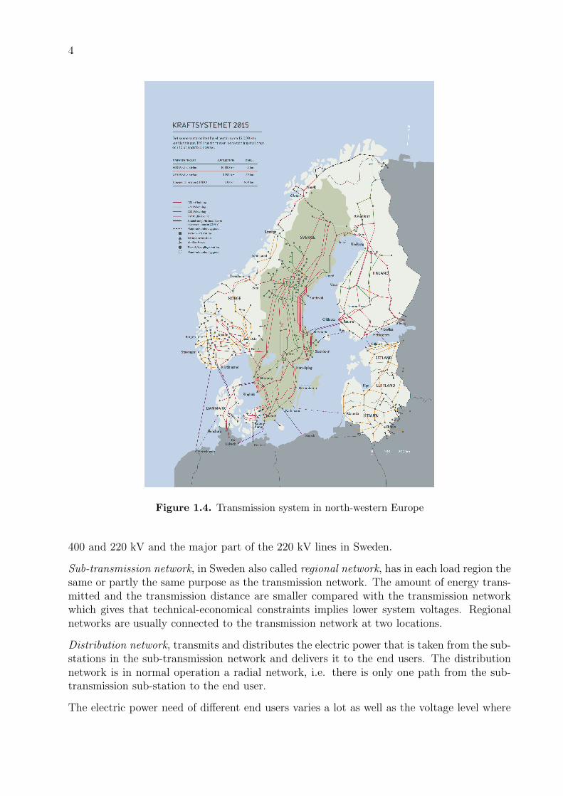
The transmission network, connects the main power sources and transmits a large amountof electric energy. The Swedish transmission system consists of approximately 15327 kmpower lines, and there are 16 interconnections to other countries. In Figure 1.4, a generalmap of the transmission system in Sweden and neighboring countries is given. The primarytask for the transmission system is to transmit energy from generation areas to load areas.To achieve a high degree of efficiency and reliability, different aspects must be taken intoaccount. The transmission system should for instance make it possible to optimize thegeneration within the country and also support trading with electricity with neighboringcountries. It is also necessary to withstand different disturbances such as disconnection oftransmission lines, lightning storms, outage of power plants as well as unexpected growthin power demand without reducing the quality of the electricity services. As shown inFigure 1.4, the transmission system is meshed, i.e. there are a number of closed loops in thetransmission system.
A state utility, Svenska Kraftnat, manages the national transmission system and foreignlinks in operation at date. Svenska Kraftnat owns all 400 kV lines, all transformers between
4
Figure 1.4. Transmission system in north-western Europe
400 and 220 kV and the major part of the 220 kV lines in Sweden.
Sub-transmission network, in Sweden also called regional network, has in each load region thesame or partly the same purpose as the transmission network. The amount of energy trans-mitted and the transmission distance are smaller compared with the transmission networkwhich gives that technical-economical constraints implies lower system voltages. Regionalnetworks are usually connected to the transmission network at two locations.
Distribution network, transmits and distributes the electric power that is taken from the sub-stations in the sub-transmission network and delivers it to the end users. The distributionnetwork is in normal operation a radial network, i.e. there is only one path from the sub-transmission sub-station to the end user.
The electric power need of different end users varies a lot as well as the voltage level where

5
the end user is connected. Generally, the higher power need the end user has, the highervoltage level is the user connected to.
The nominal voltage levels (Root Mean Square (RMS) value for tree-phase line-to-line (LL)voltages) used in distribution of high voltage electric power is normally lower compared withthe voltage levels used in transmission. In Figure 1.5, the voltage levels used in Sweden aregiven. In special industry networks, except for levels given in Figure 1.5, also the voltage660 V as well as the non-standard voltage 500 V are used. Distribution of low voltage electricpower to end users is usually performed in three-phase lines with a zero conductor, whichgives the voltage levels 400/230 V (line-to-line (LL)/line-to-neutral (LN) voltage).
transmission
network
sub-transmission
network
distribution network
high voltage
distribution network
low voltage
Nominal
voltage
kV
1000
800
400
220
800
400
200
Notation
132
66
45
130
70
50
33
22
11
6.6
3.3
30
20
10
6
3
400/230 V
ultra high
voltage (UHV)
extra high
voltage (EHV)
high voltage
industry network
only
low voltage
Figure 1.5. Standard voltage level for transmission and distribution. In Sweden,400 kV is the maximum voltage

6

Chapter 2
Alternating current circuits
In this chapter, instantaneous and also complex power in an alternating current (AC) circuitis discussed. Also, the fundamental properties of AC voltage, current and power in a balanced(or symmetrical) three-phase circuit are presented.
2.1 Single-phase circuit
Assume that an AC voltage source with a sinusoidal voltage supplies a load as shown inFigure 2.1.
( )u t
( )i t
+
-~ Load
Figure 2.1. A sinusoidal voltage source supplies a load.
Let the instantaneous voltage and current be given by
u(t) = UM cos(ωt+ θ)
i(t) = IM cos(ωt+ γ)(2.1)
where,
UM is the peak value of the voltage,
IM is the peak value of the current,
θ is the the phase angle of the voltage,
γ is the the phase angle of the current,
ω = 2π f, and f is the frequency of the voltage source.
The single-phase instantaneous power consumed by the load is given by
p(t) = u(t) · i(t) = UMIM cos(ωt+ θ) cos(ωt+ γ) =
=1
2UMIM [cos(θ − γ) + cos(2ωt+ θ + γ)] =
=UM√2
IM√2[(1 + cos(2ωt+ 2θ)) cosφ+ sin(2ωt+ 2θ) sinφ] =
= P (1 + cos(2ωt+ 2θ)) +Q sin(2ωt+ 2θ)
(2.2)
7

8
where
φ = θ − γ
P =UM√2
IM√2cosφ = U I cosφ = active power
Q =UM√2
IM√2sinφ = U I sin φ = reactive power
U and I are the Root Mean Square (RMS) value of the voltage and current, respectively.The RMS-values are defined as
U =
√
1
T
∫ T
0
u(t)2dt (2.3)
I =
√
1
T
∫ T
0
i(t)2dt (2.4)
With sinusoidal voltage and current, according to equation (2.1), the corresponding RMS-values are given by
U =
√
1
T
∫ T
0
U2M cos2(ωt+ θ) = UM
√
1
T
∫ T
0
(1
2+
cos(2ωt+ 2θ)
2
)
=UM√2
(2.5)
I =
√
1
T
∫ T
0
I2M cos2(ωt+ γ) =IM√2
(2.6)
As shown in equation (2.2), the instantaneous power has been decomposed into two com-ponents. The first component has a mean value P , and pulsates with the double frequency.The second component also pulsates with double frequency with a amplitude Q, but it hasa zero mean value. In Figure 2.2, the instantaneous voltage, current and power are shown.
time (t)
i(t)
u(t)
p(t)
UIcosφ
p(t)
time (t)
I
II
UIsinφ
UIcosφ
φ
Figure 2.2. Voltage, current and power versus time.
9
Example 2.1 A resistor of 1210 Ω is fed by an AC voltage source with frequency 50 Hz andvoltage 220 V (RMS). Find the mean value power (i.e. the active power) consumed by theresistor.
Solution
The consumed mean value power over one period can be calculated as
P =1
T
∫ T
0
p(t) dt =1
T
∫ T
0
R · i2(t)dt = 1
T
∫ T
0
Ru2(t)
R2dt =
1
R
1
T
∫ T
0
u2(t)dt
which can be rewritten according to equation (2.3) as
P =1
RU2 =
2202
1210= 40 W
2.1.1 Complex power
The complex method is a powerful tool for calculation of electrical power, and can offersolutions in an elegant manner.
The single-phase phasor voltage and current are expressed by
U = Uejθ
I = Iejγ(2.7)
where, U is the magnitude (RMS-value) of the voltage phasor, and θ is its phase angle. Also,I is the magnitude (RMS-value) of the current phasor, and γ is its phase angle.
The complex power (S) is expressed by
S = Sejφ = P + jQ = U I∗= UIej(θ−γ) = UIejφ = UI(cos φ+ j sinφ) (2.8)
which implies that
P = S cosφ = UI cosφ
Q = S sinφ = UI sin φ(2.9)
where, P is called active power, Q is called reactive power and cos φ is called power factor.
Example 2.2 Calculate the complex power consumed by an inductor with the inductanceof 3.85 H which is fed by an AC voltage source with the phasor U = U 6 θ = 220 6 0 V. Thecircuit frequency is 50 Hz.
Solution

10
The impedance is given by
Z = jωL = j · 2 · π · 50 · 3.85 = j1210 Ω
Next, the phasor current through the impedance can be calculated as
I =U
Z=
220
j1210= −j0.1818 A = 0.1818 e−j π
2 A
Thus, the complex power is given by
S = U I∗= UIej(θ−γ) = UIej(φ)
= 220 (0.1818) ej(0+π2) = 220(j0.1818) = j40 VA
i.e. P = 0 W, Q = 40 VAr.
Example 2.3 Two series connected impedances are fed by an AC voltage source with thephasor U 1 = 1 6 0 V as shown in Figure 2.3.
1 2
1 1U V=1 0.1 0.2Z j= + Ω
2 2 2U U θ= ∠
2 0.7 0.2Z j= + ΩI
Figure 2.3. Network used in Example 2.3.
a) Calculate the power consumed by Z2 as well as the power factor (cosφ) at bus 1 and 2where φk is the phase angle between the voltage and the current at bus k.
b) Calculate the magnitude U2 when Z2 is capacitive : Z2 = 0.7− j0.5 Ω
Solution
a)
U 1 = U1 6 θ1 = 1 6 0 V and I =U1
Z1 + Z2
= I 6 γ = 1.118 6 − 26.57 A
Thus, φ1 = θ1 − γ = 26.57, and cosφ1 = 0.8944 lagging, since the current lags the voltage.Furthermore,
U 2 = Z2 · I = U2 6 θ2 = 0.814 6 − 10.62
Thus, φ2 = θ2 − γ = −10.62 + 26.57 = 15.95, and cos φ2 = 0.9615, lagging. The equationabove can be written on polar form as
U2 = Z2 · Iθ2 = arg(Z2) + γ

11
U 1
−R1 · I
U 2 = U 1 −R1 · I − jX1 · I
I
γ
φ2
θ2
Figure 2.4. Solution to Example 2.3 a).
i.e. φ2 = arg(Z2) = arctan X2
R2= 15.95
The power consumption in Z2 can be calculated as
S2 = P2 + jQ2 = Z2 · I2 = (0.7 + j0.2)1.1182 = 0.875 + j0.25 VA
or
S2 = P2 + jQ2 = U 2I∗= U2 I 6 φ2 = 0.814 · 1.118 6 15.95 = 0.875 + j0.25 VA
1 2
1 1U V=1 0.1 0.2Z j= + Ω
2 2 2U U θ= ∠
2 0.7 0.5Z j= − ΩI
Figure 2.5. Network used in Example 2.3 b).
b)
U2 =
∣∣∣∣
Z2
Z1 + Z2
∣∣∣∣U1 =
|0.7− j0.5||0.8− j0.3| =
√0.49 + 0.25√0.64 + 0.09
=
√0.74√0.73
= 1.007 V
Conclusions from this example are that
• a capacitance increases the voltage - so called phase compensation,
• active power can be transmitted towards higher voltage magnitude,
• the power factor cos φ may be different in different ends of a line,
• the line impedances are ≪ load impedances.
12
2.2 Balanced three-phase circuit
In a balanced (or symmetrical) three-phase circuit, a three-phase voltage source consists ofthree AC voltage sources (one for each phase) which are equal in amplitude (or magnitude)and displaced in phase by 120. Furthermore, each phase is equally loaded.
Let the instantaneous phase (also termed as line-to-neutral (LN)) voltages be given by
ua(t) = UM cos(ωt+ θ)
ub(t) = UM cos(ωt+ θ − 2π
3) (2.10)
uc(t) = UM cos(ωt+ θ +2π
3)
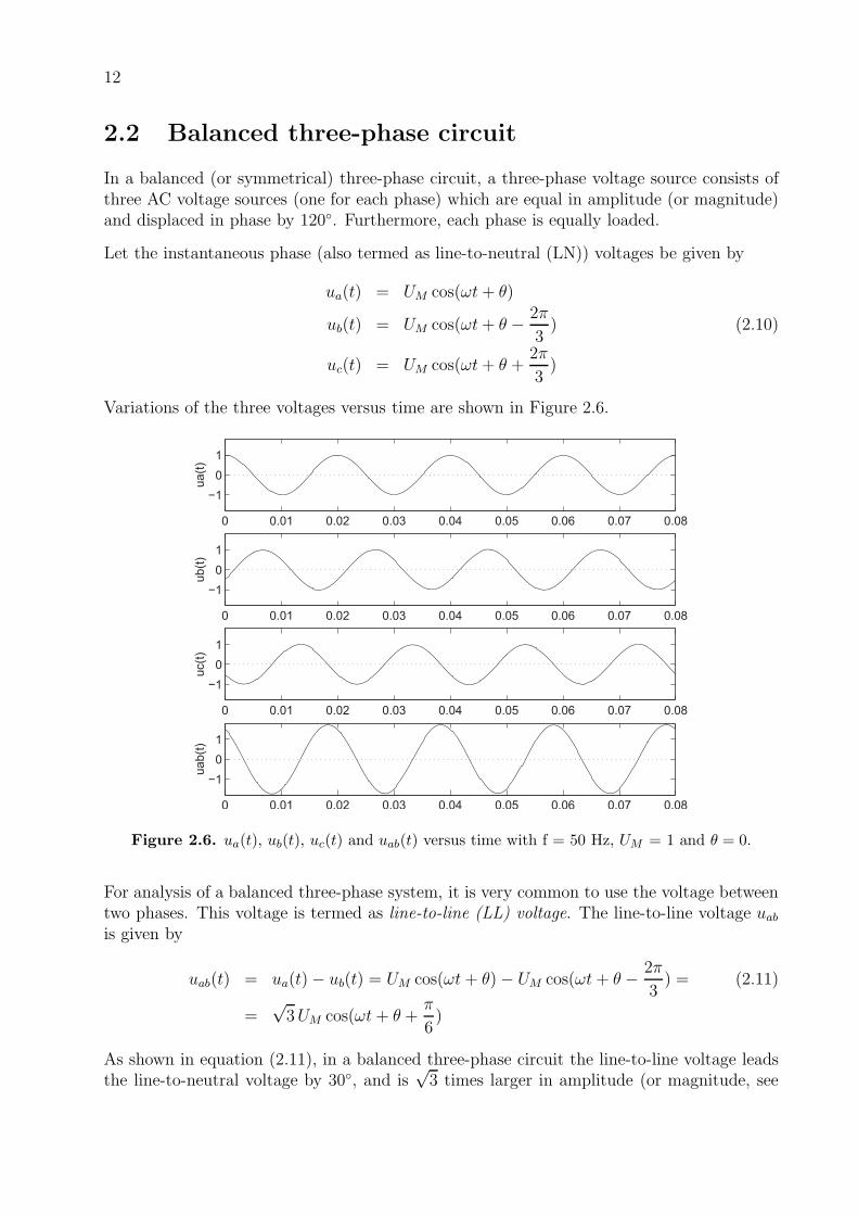
Variations of the three voltages versus time are shown in Figure 2.6.
0 0.01 0.02 0.03 0.04 0.05 0.06 0.07 0.08
−1
0
1
ua(t
)
0 0.01 0.02 0.03 0.04 0.05 0.06 0.07 0.08
−1
0
1
ub(t
)
0 0.01 0.02 0.03 0.04 0.05 0.06 0.07 0.08
−1
0
1
uc(t
)
0 0.01 0.02 0.03 0.04 0.05 0.06 0.07 0.08
−1
0
1
uab(t
)
Figure 2.6. ua(t), ub(t), uc(t) and uab(t) versus time with f = 50 Hz, UM = 1 and θ = 0.
For analysis of a balanced three-phase system, it is very common to use the voltage betweentwo phases. This voltage is termed as line-to-line (LL) voltage. The line-to-line voltage uab
is given by
uab(t) = ua(t)− ub(t) = UM cos(ωt+ θ)− UM cos(ωt+ θ − 2π
3) = (2.11)
=√3UM cos(ωt+ θ +
π
6)
As shown in equation (2.11), in a balanced three-phase circuit the line-to-line voltage leadsthe line-to-neutral voltage by 30, and is
√3 times larger in amplitude (or magnitude, see

13
equation (2.5)). For instance, at a three-phase power outlet the magnitude of a phase is 230V, but the magnitude of a line-to-line voltage is
√3 · 230 = 400 V, i.e. ULL =
√3ULN . The
line-to-line voltage uab is shown at the bottom of Figure 2.6.
Next, assume that the voltages given in equation (2.10) supply a balanced (or symmetrical)three-phase load whose phase currents are
ia(t) = IM cos(ωt+ γ)
ib(t) = IM cos(ωt+ γ − 2π
3) (2.12)
ic(t) = IM cos(ωt+ γ +2π
3)
Then, the total instantaneous power is given by
p3(t) = pa(t) + pb(t) + pc(t) = ua(t)ia(t) + ub(t)ib(t) + uc(t)ic(t) =
=UM√2
IM√2[(1 + cos 2(ωt+ θ)) cosφ+ sin 2(ωt+ θ) sinφ] +
+UM√2
IM√2[(1 + cos 2(ωt+ θ − 2π
3)) cosφ+ sin 2(ωt+ θ − 2π
3) sinφ] +
+UM√2
IM√2[(1 + cos 2(ωt+ θ +
2π
3)) cosφ+ sin 2(ωt+ θ +
2π
3) sinφ] = (2.13)
= 3UM√2
IM√2
[
cosφ+
(
cos 2(ωt+ θ) + cos 2[ωt+ θ − 2π
3] + cos 2[ωt+ θ +
2π
3]
)
︸ ︷︷ ︸
=0
+
+
(
sin 2(ωt+ θ) + sin 2[ωt+ θ − 2π
3] + sin 2[ωt+ θ +
2π
3]
)
︸ ︷︷ ︸
=0
]
=
= 3UM√2
IM√2cos φ = 3ULN I cosφ
Note that the total instantaneous power is equal to three times the active power of a singlephase, and it is constant. This is one of the main reasons why three-phase systems havebeen used.
2.2.1 Complex power
The corresponding phasor voltages are defined as:
Ua = ULN 6 θ
U b = ULN 6 (θ − 120) (2.14)
U c = ULN 6 (θ + 120)
Figure 2.7 shows the phasor diagram of the three balanced line-to-neutral voltages, and alsothe phasor diagram of the line-to-line voltages.

14
cU
caU
aU
abUbU
bcU
120+ °
120- °
Figure 2.7. Phasor diagram of the line-to-neutral and line-to-line voltages.
The phasor of the line-to-line voltages can be determined as follows
Uab =Ua − U b =√3ULN 6 (θ + 30) =
√3Ua e
j30
U bc =U b − U c =√3ULN 6 (θ − 90) =
√3U b e
j30
U ca =U c − Ua =√3ULN 6 (θ + 150) =
√3U c e
j30
(2.15)
Obviously, the line-to-line voltages are also balanced. Equation (2.15) also shows that theline-to-line phasor voltage leads the line-to-neutral phasor voltage by 30, and it is
√3 times
the line-to-neutral phasor voltage.
Next, let the balanced phasor currents be defined as
Ia = I 6 γ
Ib = I 6 (γ − 120) (2.16)
Ic = I 6 (γ + 120)
Then, the total three-phase power (S3Φ) is given by :
S3Φ = Sa + Sb + Sc = UaI∗a + U bI
∗b + U cI
∗c =
= 3ULN I cosφ+ j3ULN I sin φ =
= 3ULN I ejφ(2.17)
Obviously, for a balanced three-phase system Sa = Sb = Sc and S3Φ = 3S1Φ, where S1Φ isthe complex power of a single phase.
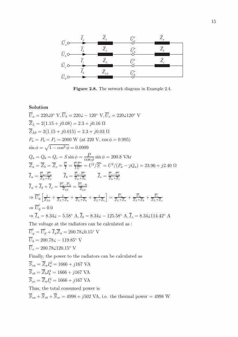
Example 2.4 The student Elektra lives in a house situated 2 km from a transformer havinga completely symmetrical three-phase voltage (Ua = 220V 6 0, U b = 220V 6 − 120, U c =220V 6 120 ). The house is connected to this transformer via a three-phase cable (EKKJ,3×16 mm2 + 16 mm2). A cold day, Elektra switches on two electrical radiators to eachphase, each radiator is rated 1000 W (at 220 V with cosφ = 0.995 lagging (inductive)).Assume that the cable can be modeled as four impedances connected in parallel (zL = 1.15 +j0.08 Ω/phase,km, zL0 = 1.15 + j0.015 Ω/km) and that the radiators also can be consideredas impedances. Calculate the total thermal power given by the radiators.
15
LZ
aI aU ′
bU ′
cU ′
0U ′
aU
bU
cU
0U
bI
cI
0I
LZ
0LZ
aZ
bZ
cZ
LZ
Figure 2.8. The network diagram in Example 2.4.
Solution
Ua = 220 6 0 V, U b = 220 6 − 120 V, U c = 220 6 120 V
ZL = 2(1.15 + j0.08) = 2.3 + j0.16 Ω
ZL0 = 2(1.15 + j0.015) = 2.3 + j0.03 Ω
Pa = Pb = Pc = 2000 W (at 220 V, cosφ = 0.995)
sinφ =√
1− cos2 φ = 0.0999
Qa = Qb = Qc = S sinφ = Pcosφ
sin φ = 200.8 VAr
Za = Zb = Zc =UI= U ·U∗
I·U∗ = U2/S∗= U2/(Pa − jQa) = 23.96 + j2.40 Ω
Ia =Ua−U
′
0
ZL+ZaIb =
Ub−U′
0
ZL+ZbIc =
Uc−U′
0
ZL+Zc
Ia + Ib + Ic =U
′
0−U0
ZL0= U
′
0−0
ZL0
⇒ U′0
[1
ZL0+ 1
ZL+Za+ 1
ZL+Zb+ 1
ZL+Zc
]
= Ua
ZL+Za+ Ub
ZL+Zb+ Uc
ZL+Zc
⇒ U′0 = 0.0
⇒ Ia = 8.34 6 − 5.58 A, Ib = 8.34 6 − 125.58 A, Ic = 8.34 6 114.42 A
The voltage at the radiators can be calculated as :
U′a = U
′0 + IaZa = 200.78 6 0.15 V
U b = 200.78 6 − 119.85 V
U c = 200.78 6 120.15 V
Finally, the power to the radiators can be calculated as
Sza = ZaI2a = 1666 + j167 VA
Szb = ZbI2b = 1666 + j167 VA
Szc = ZaI2c = 1666 + j167 VA
Thus, the total consumed power is
Sza + Szb + Szc = 4998 + j502 VA, i.e. the thermal power = 4998 W

16
Note that since we are dealing with a balanced three-phase system, Sza = Szb = Szc.
The total transmission losses are
ZL(I2a + I2b + I2c ) + ZL0|Ia + Ib + Ic|2) = ZL(I
2a + I2b + I2c ) = 480 + j33 VA
i.e. the active losses are 480 W, which means that the efficiency is 91.2 %.
In a balanced three-phase system, Ia + Ib + Ic = 0. Thus, no current flows in the neutralconductor (i.e. I0 = 0), and the voltage at the neutral point is zero, i.e. U
′0 = 0. Therefore,
for analyzing a balanced three-phase system, it is more common to analyze only a singlephase (or more precisely only the positive-sequence network of the system, see Chapter 8).Then, the total three-phase power can be determined as three times the power of the singlephase.
Example 2.5 Use the data in Example 2.4, but in this example the student Elektra connectsone 1000 W radiator (at 220 V with cosφ = 0.995 lagging) to phase a, three radiators tophase b and two to phase c. Calculate the total thermal power given by the radiators, as wellas the system losses.
Solution
Ua = 220 6 0 V, U b = 220 6 − 120 V, U c = 220 6 120 V
ZL = 2(1.15 + j0.08) = 2.3 + j0.16 Ω
ZL0 = 2(1.15 + j0.015) = 2.3 + j0.03 Ω
Pa = 1000 W (at 220 V, cosφ = 0.995)
sinφ =√
1− cos2 φ = 0.0999
Qa = S sinφ = Pcosφ
sin φ = 100.4 VAr
Za = U2/S∗a = U2/(Pa − jQa) = 47.9 + j4.81 Ω
Zb = Za/3 = 15.97 + j1.60 Ω
Zc = Za/2 = 23.96 + j2.40 Ω
U′0
[1
ZL0+ 1
ZL+Za+ 1
ZL+Zb+ 1
ZL+Zc
]
= Ua
ZL+Za+ Ub
ZL+Zb+ Uc
ZL+Zc
⇒ U′0 = 12.08 6 − 155.14 V
⇒ Ia = 4.58 6 − 4.39 A, Ib = 11.45 6 − 123.62 A, Ic = 8.31 6 111.28 A
The voltages at the radiators can be calculated as :
U′a = U
′0 + IaZa = 209.45 6 0.02 V
U′b = U
′0 + IbZb = 193.60 6 − 120.05 V
U′c = U
′0 + IcZc = 200.91 6 129.45 V
Note that these voltages are not local phase voltages since they are calculated as U′a − U
′0
etc. The power to the radiators can be calculated as :
Sza = ZaI2a = 1004 + j101 VA

17
Szb = ZbI2b = 2095 + j210 VA
Szc = ZaI2c = 1655 + j166 VA
The total amount of power consumed is
Sza + Szb + Szc = 4754 + j477 VA, i.e. the thermal power is 4754 W
The total transmission losses are
ZL(I2a + I2b + I2c ) + ZL0|Ia + Ib + Ic|2) = 572.1 + j36 VA, i.e. 572.1 W
which gives an efficiency of 89.3 %.
As shown in this example, an unsymmetrical impedance load will result in unsymmetricalphase currents, i.e. we are dealing with an unbalanced three-phase system. As a consequence,a voltage can be detected at the neutral point (i.e. U
′0 6= 0) which gives rise to a current
in the neutral conductor, i.e. I0 6= 0. The total thermal power obtained was reduced byapproximately 5 % and the line losses increased partly due to the losses in the neutralconductor. The efficiency of the transmission decreased. It can also be noted that the powerper radiator decreased with the number of radiators connected to the same phase. This owingto the fact that the voltage at the neutral point will be closest to the voltage in the phasewith the lowest impedance, i.e. the phase with the largest number of radiators connected.

18

Chapter 3
Models of power system components
Electric energy is transmitted from power plants to consumers via overhead lines, cables andtransformers. In the following, these components will be discussed and mathematical modelsto be used in the analysis of symmetrical three-phase systems will be derived. In Chapter8, analysis of power systems under unsymmetrical conditions will be discussed.
3.1 Electrical characteristic of an overhead line
Overhead transmission lines need large surface area and are mostly suitable to be used inrural areas and in areas with low population density. In areas with high population densityand urban areas cables are a better alternative. For a certain amount of power transmitted,a cable transmission system is about ten times as expensive as an overhead transmissionsystem.
Power lines have a resistance (r) owing to the resistivity of the conductor and a shunt con-ductance (g) because of leakage currents in the insulation. The lines also have an inductance(l) owing to the magnetic flux surrounding the line as well as a shunt capacitance (c) becauseof the electric field between the lines and between the lines and ground. These quantitiesare given per unit length and are continuously distributed along the whole length of the line.Resistance and inductance are in series while the conductance and capacitance are shuntquantities.
l l l lr r r r
c c c cg g g g
Figure 3.1. A line with distributed quantities.
Assuming symmetrical three-phase, a line can be modeled as shown in Figure 3.1. Thequantities r, g, l, and c determine the characteristics of a line. Power lines can be modeledby simple equivalent circuits which, together with models of other system components, canbe formed to a model of a complete system or parts of it. This is important since suchmodels are used in power system analysis where active and reactive power flows in thenetwork, voltage levels, losses, power system stability and other properties at disturbancesas e.g. short circuits, are of interest.
For a more detailed derivation of the expressions of inductance and capacitance given below,more fundamental literature in electro-magnetic theory has to be studied.
19

20
3.1.1 Resistance
The resistance of a conductor with the cross-section area A mm2 and the resistivity ρΩmm2/km is
r =ρ
AΩ/km (3.1)
The conductor is made of copper with the resistivity at 20C of 17.2 Ωmm2/km, or aluminumwith the resistivity at 20C of 27.0 Ωmm2/km. The choice between copper or aluminum isrelated to the price difference between the materials.
The effective alternating current resistance at normal system frequency (50–60 Hz) for lineswith a small cross-section area is close to the value for the direct current resistance. Forlarger cross-section areas, the current density will not be equal over the whole cross-section.The current density will be higher at the peripheral parts of the conductor. That phenomenais called current displacement or skin effect and depends on the internal magnetic flux ofthe conductor. The current paths that are located in the center of the conductor will besurrounded by the whole internal magnetic flux and will consequently have an internal selfinductance. Current paths that are more peripheral will be surrounded by a smaller magneticflux and thereby have a smaller internal inductance.
The resistance of a line is given by the manufacturer where the influence of the skin effect istaken. Normal values of the resistance of lines are in the range 10–0.01 Ω/km.
The resistance plays, compared with the reactance, often a minor role when comparing thetransmission capability and voltage drop between different lines. For low voltage lines andwhen calculating the losses, the resistance is of significant importance.
3.1.2 Shunt conductance
The shunt conductance of an overhead line represents the losses owing to leakage currentsat the insulators. There are no reliable data over the shunt conductances of lines and theseare very much dependent on humidity, salt content and pollution in the surrounding air. Forcables, the shunt conductance represents the dielectric losses in the insulation material anddata can be obtained from the manufacturer.
The dielectric losses are e.g. for a 12 kV cross-linked polyethylene (XLPE) cable with across-section area of 240 mm2/phase 7 W/km,phase and for a 170 kV XLPE cable with thesame area 305 W/km,phase.
The shunt conductance will be neglected in all calculations throughout this compendium.
3.1.3 Inductance
The inductance is in most cases the most important parameter of a line. It has a largeinfluence on the line transmission capability, voltage drop and indirectly the line losses. Theinductance of a line can be calculated by the following formula :

21
l = 2 · 10−4
(
lna
d/2+
1
4n
)
H/km,phase (3.2)
where
a = 3√a12a13a23 m, = geometrical mean distance according to Figure 3.2.
d = diameter of the conductor, m
n = number of conductors per phase
Ground level
H1
H2 H
3
a12
a23
a13
A1
A2
A3
Figure 3.2. The geometrical quantities of a line in calculations of inductance and capacitance.
The calculation of the inductance according to equation (3.2), is made under some assump-tions, viz. the conductor material must be non-magnetic as copper and aluminum togetherwith the assumption that the line is transposed. The majority of the long transmission linesare transposed, see Figure 3.3.
Transposing cycle
Locations of transposing
Figure 3.3. Transposing of three-phase overhead line.
This implies that each one of the conductors, under a transposing cycle, has had all threepossible locations in the transmission line. Each location is held under equal distance whichimplies that all conductors in average have the same distance to ground and to the otherconductors. This gives that the mutual inductance between the three phases are equalizedso that the inductance per phase is equal among the three phases.
22
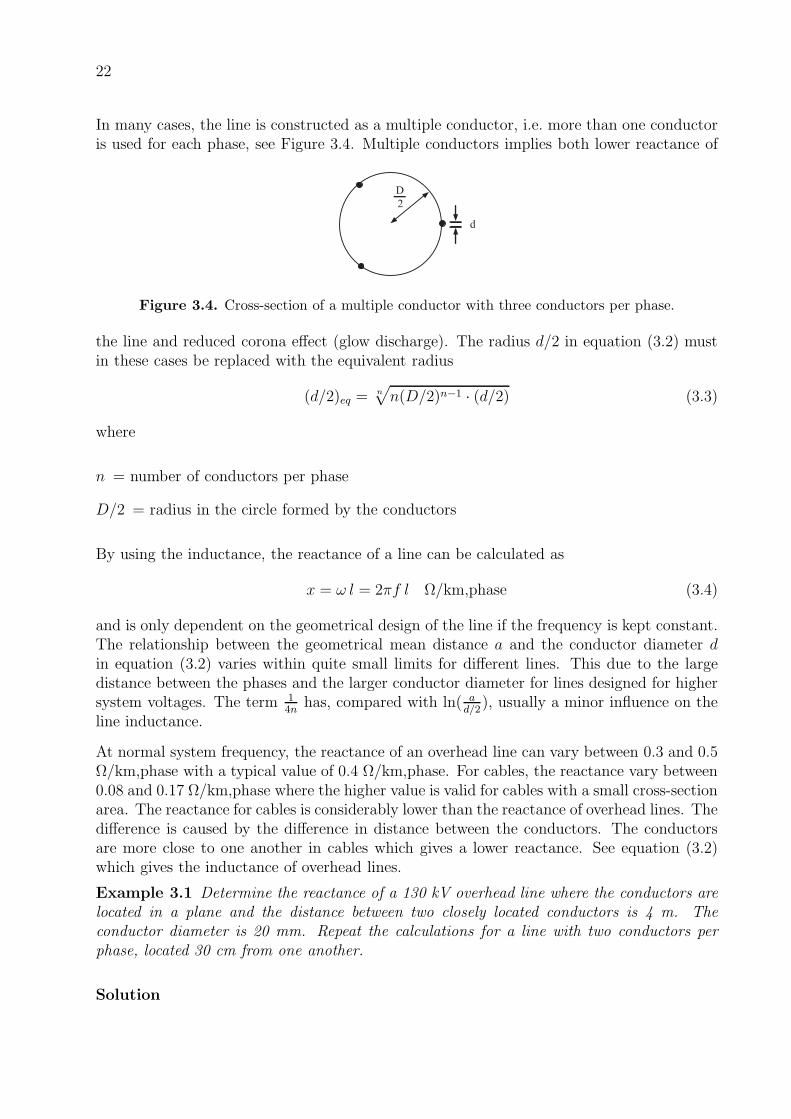
In many cases, the line is constructed as a multiple conductor, i.e. more than one conductoris used for each phase, see Figure 3.4. Multiple conductors implies both lower reactance of
D
2
d
Figure 3.4. Cross-section of a multiple conductor with three conductors per phase.
the line and reduced corona effect (glow discharge). The radius d/2 in equation (3.2) mustin these cases be replaced with the equivalent radius
(d/2)eq =n√
n(D/2)n−1 · (d/2) (3.3)
where
n = number of conductors per phase
D/2 = radius in the circle formed by the conductors
By using the inductance, the reactance of a line can be calculated as
x = ω l = 2πf l Ω/km,phase (3.4)
and is only dependent on the geometrical design of the line if the frequency is kept constant.The relationship between the geometrical mean distance a and the conductor diameter din equation (3.2) varies within quite small limits for different lines. This due to the largedistance between the phases and the larger conductor diameter for lines designed for highersystem voltages. The term 1
4nhas, compared with ln( a
d/2), usually a minor influence on the
line inductance.
At normal system frequency, the reactance of an overhead line can vary between 0.3 and 0.5Ω/km,phase with a typical value of 0.4 Ω/km,phase. For cables, the reactance vary between0.08 and 0.17 Ω/km,phase where the higher value is valid for cables with a small cross-sectionarea. The reactance for cables is considerably lower than the reactance of overhead lines. Thedifference is caused by the difference in distance between the conductors. The conductorsare more close to one another in cables which gives a lower reactance. See equation (3.2)which gives the inductance of overhead lines.
Example 3.1 Determine the reactance of a 130 kV overhead line where the conductors arelocated in a plane and the distance between two closely located conductors is 4 m. Theconductor diameter is 20 mm. Repeat the calculations for a line with two conductors perphase, located 30 cm from one another.
Solution

23
a12 = a23 = 4, a13 = 8
d/2 = 0.01 m
a = 3√4 · 4 · 8 = 5.04
x = 2π · 50 · 2 · 10−4(ln 5.04
0.01+ 1
4
)= 0.0628 (ln(504) + 0.25) = 0.41 Ω/km,phase
Multiple conductor (duplex)
(d/2)eq =2√
2(0.3/2)0.01 = 0.055
x = 0.0628(ln 5.04
0.055+ 1
8
)= 0.29 Ω/km,phase
The reactance is in this case reduced by 28 %.
3.1.4 Shunt capacitance
For a three-phase transposed overhead line, the capacitance to ground per phase can becalculated as
c =10−6
18 ln(
2HA
· a(d/2)eq
) F/km,phase (3.5)
where
H = 3√H1H2H3 = geometrical mean height for the conductors according to Figure 3.2.
A = 3√A1A2A3 = geometrical mean distance between the conductors and their image con-
ductors according to Figure 3.2.
As indicated in equation (3.5), the ground has some influence on the capacitance of the line.The capacitance is determined by the electrical field which is dependent on the characteristicsof the ground. The ground will form an equipotential surface which has an influence on theelectric field.
The degree of influence the ground has on the capacitance is determined by the factor 2H/Ain equation (3.5). This factor has usually a value near 1.
Assume that a line mounted on relatively high poles (⇒ A ≈ 2H) is considered and that theterm 1
4ncan be neglected in equation (3.2). By multiplying the expressions for inductance
and capacitance, the following is obtained
l · c = 2 · 10−4
(
lna
(d/2)eq
)
· 10−6
18 ln(
a(d/2)eq
) =1
(3 · 105)2(km
s
)−2
=1
v2(3.6)
where v = speed of light in vacuum in km/s. Equation (3.6) can be interpreted as theinductance and capacitance are the inverse of one another for a line. Equation (3.6) is agood approximation for an overhead line. The shunt susceptance of a line is
bc = 2πf · c S/km,phase (3.7)
A typical value of the shunt susceptance of a line is 3 · 10−6 S/km,phase. Cables haveconsiderable higher values between 3 · 10−5 – 3 · 10−4 S/km,phase.

24
Example 3.2 Assume that a line has a shunt susceptance of 3 · 10−6 S/km,phase. Useequation (3.6) to estimate the reactance of the line.
Solution
x = ωl ≈ ω
cv2=
ω2
bv2=
(100π)2
3 · 10−6(3 · 105)2 = 0.366 Ω/km
which is near the standard value of 0.4 Ω/km for the reactance of an overhead line.
3.2 Model of a line
Both overhead lines and cables have their electrical quantities r, x, g and b distributed alongthe whole length. Figure 3.1 shows an approximation of the distribution of the quantities.Generally, the accuracy of the calculation result will increase with the number of distributedquantities.
At a first glance, it seems possible to form a line model where the total resistance/inductanceis calculated as the product between the resistance/inductance per length unit and the lengthof the line. This approximation is though only valid for short lines and lines of mediumlength. For long lines, the distribution of the quantities r, l, c and g must be taken intoaccount. Such analysis can be carried out with help of differential calculus.
There are no absolute limits between short, medium and long lines. Usually, lines shorterthan 100 km are considered as short, between 100 km and 300 km as medium long and lineslonger than 300 km are classified as long. For cables, having considerable higher values ofthe shunt capacitance, the distance 100 km should be considered as medium long. In thefollowing, models for short and medium long lines are given.
3.2.1 Short lines
In short line models, the shunt parameters are neglected, i.e. conductance and susceptance.This because the current flowing through these components is less than one percent of therated current of the line. The short line model is given in Figure 3.5. This single-phasemodel of a three-phase system is valid under the assumption that the system is operatingunder symmetrical conditions.
kUkI kj kj kjZ R jX= +
jU
Figure 3.5. Short line model of a line.

25
The impedance of the line between bus k and bus j can be calculated as
Zkj = Rkj + jXkj = (rkj + jxkj)L Ω/phase (3.8)
where L is the length of the line in km.
3.2.2 Medium long lines
For lines having a length between 100 and 300 km, the shunt capacitance cannot be neglected.The model shown in Figure 3.5 has to be extended with the shunt susceptance, whichresults in a model called the π-equivalent shown in Figure 3.6. The impedance is calculated
kUkI
kj kj kjZ R jX= +
jU
2
sh kjY −
2
sh kjY −
shI
I
or
kUkI
kj kj kjZ R jX= +
jU
sh kjy −
shI
I
sh kjy −
Figure 3.6. Medium long model of a line.
according to equation (3.8) and the admittance to ground per phase is obtained by
Y sh−kj
2= j
bc L2
= ysh−kj = jbsh−kj S (3.9)
i.e. the total shunt capacitance of the line is divided into two equal parts, one at each endof the line. The π-equivalent is a very common and useful model in power system analysis.
3.3 Single-phase transformer
The principle diagram of a two winding transformer is shown in Figure 3.7. The fundamentalprinciples of a transformer are given in the figure. In a real transformer, the demand ofa strong magnetic coupling between the primary and secondary sides must be taken intoaccount in the design.
Assume that the magnetic flux can be divided into three components. There is a core flux Φm
passing through both the primary and the secondary windings. There are also leakage fluxes,Φl1 passing only the primary winding and Φl2 which passes only the secondary winding. Theresistance of the primary winding is r1 and for the secondary winding r2. According to thelaw of induction, the following relationships can be given for the voltages at the transformerterminals :
u1 = r1i1 +N1d(Φl1 + Φm)
dt(3.10)
u2 = r2i′2 +N2
d(Φl2 + Φm)
dt

26
Iron core
mΦ
1lΦ
2lΦ
1u
2u
1i 2
i′
Primary
Winding
N1 turns
Secondary
Winding
N2 turns
Figure 3.7. Principle design of a two winding transformer.
Assuming linear conditions, the following is valid
N1Φl1 = Ll1i1 (3.11)
N2Φl2 = Ll2i′2
where
Ll1 = inductance of the primary winding
Ll2 = inductance of the secondary winding
Equation (3.10) can be rewritten as
u1 = r1i1 + Ll1di1dt
+N1dΦm
dt(3.12)
u2 = r2i′2 + Ll2
di′2dt
+N2dΦm
dt
With the reluctance R of the iron core and the definitions of the directions of the currentsaccording to Figure 3.7, the magnetomotive forces N1i1 and N2i
′2 can be added as
N1i1 +N2i′2 = RΦm (3.13)
Assume that i′2 = 0, i.e. the secondary side of the transformer is not connected. The currentnow flowing in the primary winding is called the magnetizing current and the magnitude canbe calculated using equation (3.13) as
im =RΦm
N1(3.14)

27
If equation (3.14) is inserted into equation (3.13), the result is
i1 = im − N2
N1
i′2 = im +N2
N1
i2 (3.15)
wherei2 = −i′2 (3.16)
Assuming linear conditions, the induced voltage drop N1dΦmdt
in equation (3.12) can beexpressed by using an inductor as
N1dΦm
dt= Lm
dimdt
(3.17)
i.e. Lm = N21 /R. By using equations (3.12), (3.15) and (3.17), the equivalent diagram of a
single-phase transformer can be drawn, see Figure 3.8.
22
1
Ni
N
mi
1i 2i2r1r
1u 2u2e1e
1lL 2lL
1N 2N
mL
ideal
Figure 3.8. Equivalent diagram of a single-phase transformer.
In Figure 3.8, one part of the ideal transformer is shown, which is a lossless transformerwithout leakage fluxes and magnetizing currents.
The equivalent diagram in Figure 3.8 has the advantage that the different parts representsdifferent parts of the real transformer. For example, the inductance Lm represents theassumed linear relationship between the core flux Φm and the magnetomotive force of theiron core. Also the resistive copper losses in the transformer are represented by r1 and r2.
In power system analysis, where the transformer is modeled, a simplified model is often usedwhere the magnetizing current is neglected.
3.4 Three-phase transformer
There are three fundamental ways of connecting single-phase transformers into one three-phase transformer. The three combinations are Y-Y-connected, ∆-∆-connected and Y-∆-connected (or ∆-Y-connected). In Figure 3.9, the different combinations are shown.
When the neutral (i.e. n or N) is grounded, the Y-connected part will be designated byY0. The different consequences that these different connections imply, will be discussed inChapter 8.

28
a
b
c
n N
A
B
C
a
b
c
A
B
C
a
b
c
n
A
B
C
Y-Y-connected Y- -connected- -connected
Figure 3.9. Standard connections for three-phase transformers.
3.4.1 Single-phase equivalent of three-phase transformers
Figure 3.10 shows the single-phase equivalent of a Y-Y-connected three-phase transformer. Inthe figure, Uan and UAN are the line-to-neutral phasor voltages of the primary and secondarysides, respectively. However, Uab and UAB are the line-to-line phasor voltages of the primaryand secondary sides, respectively. As shown in Figure 3.10 b), the ratio of line-to-neutralvoltages is the same as the ratio of line-to-line voltages.
aIa
b
c
nabUanU 1N
N
ANU
A
C
B
ABU
AI 1 2:N N
anU ANU
aI AI
a) b)
1 1
2 2
;an ab
AN AB
U UN N
U N U N= =
2N
Figure 3.10. Single-phase equivalent of a three-phase Y-Y-connected transformer.
Figure 3.11 shows the single-phase equivalent of a ∆-∆-connected three-phase transformer.For a ∆-∆-connected transformer the ratio of line-to-neutral voltages is also the same asthe ratio of line-to-line voltages. Furthermore, for Y-Y-connected and ∆-∆-connected trans-formers Uan is in phase with UAN (or Uab is in phase with UAB).
It should be noted that ∆ windings have no neutral, and for analysis of ∆-connected trans-formers it is more convenient to replace the ∆-connection with an equivalent Y-connection

29
aIa
b
c
n
abUanU
1N
N
ANU
A
C
B
ABU
AI
a) b)
2N
1 2:3 3
N N
anU ANU
aI AI
1 1
22
/ 3;
/ 3
an ab
AB AB
U UN N
U U NN= =
1 / 3N 2 / 3N
Figure 3.11. Single-phase equivalent of a three-phase ∆-∆-connected transformer.
as shown with the dashed lines in the figure. Since for balanced operation, the neutrals of theequivalent Y-connections have the same potential the single-phase equivalent of both sidescan be connected together by a neutral conductor. This is also valid for Y-∆-connected (or∆-Y-connected) three-phase transformer.
Figure 3.12 shows the single-phase equivalent of a Y-∆-connected three-phase transformer.
aIa
b
c
nabUanU 1N
N
ANU
A
C
B
ABU
AI
a) b)
2N
2/ 3N
21 :
3
NN
anU ANU
aI AI
1 1
2 2
; 3an ab
AB AB
U UN N
U N U N= =
Figure 3.12. Single-phase equivalent of a three-phase Y-∆-connected transformer.
It can be shown that Uan = N1
N2UAB =
√3 N1
N2UAN ej 30
, i.e. Uan leads UAN by 30 (see alsoequation (2.15)).
In this compendium, this phase shift is not of concern. Furthermore, in this compendiumthe ratio of rated line-to-line voltages (rather than the turns ratio) will be used. Therefore,regardless of the transformer connection, the voltage and current can be transferred from thevoltage level on one side to the voltage level on the other side by using the ratio of rated line-to-line voltages as multiplying factor. Also, the transformer losses and magnetizing currents(i.e. im in Figure 3.8) are neglected.
Figure 3.13 shows the single-line diagram of a lossless three-phase transformer which will beused in this compendium. In the figure, U1n is the rated line-to-line voltage (given in kV) ofthe primary side and U2n is the rated line-to-line voltage (given in kV) of the secondary side.

30
1U
1
2
; ;nnt t
n
US x
U
2U
Figure 3.13. Single-line diagram of a three-phase transformer.
U1n/U2n is the ratio of rated line-to-line voltages. Snt is the transformer three-phase ratinggiven in MVA, and xt is the transformer leakage reactance, normally given as a percent basedon the transformer rated (or nominal) values. Finally, U1 and U 2 are the line-to-line phasorvoltages of the transformer terminals.

Chapter 4
Important theorems in power system analysis
In many cases, the use of theorems can simplify the analysis of electrical circuits and systems.In the following sections, some important theorems will be discussed and proofs will be given.
4.1 Bus analysis, admittance matrices
Consider an electric network which consists of four buses as shown in Figure 4.1. Each busis connected to the other buses via an admittance ykj where the subscript indicates whichbuses the admittance is connected to. Assume that there are no mutual inductances between
o o
o
o
y12
y23y13
y14
y24
y34
1
3
4
2I2I1
I4
I3
Figure 4.1. Four bus network.
the admittances and that the buses voltages are U 1, U 2, U 3 and U4. The currents I1, I2, I3and I4 are assumed to be injected into the buses from external current sources. Applicationof Kirchhoff’s current law at bus 1 gives
I1 = y12(U1 − U2) + y13(U1 − U 3) + y14(U 1 − U 4) (4.1)
or
I1 = (y12 + y13 + y14)U 1 − y12U 2 − y13U3 − y14U4 = (4.2)
= Y 11U 1 + Y 12U2 + Y 13U3 + Y 14U 4
where
Y 11 = y12 + y13 + y14 , Y 12 = −y12 , Y 13 = −y13 and Y 14 = −y14 (4.3)
Corresponding equations can be formed for the other buses. These equations can be put
31

32
together to a matrix equation as :
I =
I1I2I3I4
=
Y 11Y 12Y 13Y 14
Y 21Y 22Y 23Y 24
Y 31Y 32Y 33Y 34
Y 41Y 42Y 43Y 44
U 1
U 2
U 3
U 4
= YU (4.4)
This matrix is termed as the bus admittance matrix or Y-bus matrix which has the followingproperties :
• It can be uniquely determined from a given admittance network.
• The diagonal element Y kk is the sum of all admittances connected to bus k.
• The non-diagonal element Y kj is defined by Y kj = −ykj = − 1Zkj
where ykj is the
admittance between bus k and bus j.
• This gives that the matrix is symmetric, i.e. Y kj = Y jk (one exception is when thenetwork includes phase shifting transformers).
• It is singular since I1 + I2 + I3 + I4 = 0
If the potential in one bus is assumed to be zero, the corresponding row and column in theadmittance matrix can be removed which results in a non-singular matrix. Bus analysis usingthe Y-bus matrix is the method most often used when studying larger, meshed networks ina systematic manner.
Example 4.1 Re-do Example 2.5 by using the Y-bus matrix of the network in order tocalculate the power given by the radiators.
2I1U
2U
3U
3I
0I 4I4U
1I
LZ
0U
LZ
0LZ
aZ
bZ
cZ
LZ
Figure 4.2. Network diagram used in the example.
Solution
According to the task and to the calculations performed in Example 2.5, the following is valid;ZL = 2.3 + j0.16 Ω, ZL0 = 2.3 + j0.03 Ω, Za = 47.9 + j4.81 Ω, Zb = 15.97 + j1.60 Ω, Zc =

33
23.96 + j2.40 Ω. Start with forming the Y-bus matrix. I0 and U 0 are neglected since thesystem otherwise will be singular.
I =
I1I2I3I4
=
1ZL+Za
0 0 − 1ZL+Za
0 1ZL+Zb
0 − 1ZL+Zb
0 0 1ZL+Zc
− 1ZL+Zc
− 1ZL+Za
− 1ZL+Zb
− 1ZL+Zc
Y 44
U 1
U 2
U 3
U 4
= YU (4.5)
where
Y 44 =1
ZL + Za
+1
ZL + Zb
+1
ZL + Zc
+1
ZL0
(4.6)
In the matrix equation above, U 1, U 2, U3 and I4 (I4=0) as well as all impedances, i.e. theY-bus matrix, are known. If the given Y-bus matrix is inverted, the corresponding Z-busmatrix is obtained :
U =
U 1
U 2
U 3
U 4
= ZI = Y−1I =
Z11Z12Z13Z14
Z21Z22Z23Z24
Z31Z32Z33Z34
Z41Z42Z43Z44
I1I2I3I4
(4.7)
Since the elements in the Y-bus matrix are known, all the elements in the Z-bus matrix canbe calculated. Since I4=0 the voltages U1, U2 and U 3 can be expressed as a function of thecurrents I1, I2 and I3 by using only a part of the Z-bus matrix :
U 1
U 2
U 3
=
Z11Z12Z13
Z21Z22Z23
Z31Z32Z33
I1I2I3
(4.8)
Since the voltages U 1, U 2 and U 3 are known, the currents I1, I2 and I3 can be calculated as :
I1I2I3
=
Z11Z12Z13
Z21Z22Z23
Z31Z32Z33
−1
U1
U2
U3
= (4.9)
= 10−3
19.0− j1.83 −1.95− j0.324 −1.36 + j0.227−1.95 + j0.324 48.9− j4.36 −3.73− j0.614−1.36 + j0.227 −3.73 + j0.614 35.1− j3.25
220 6 0
220 6 − 120
220 6 120
=
=
4.58 6 − 4.39
11.5 6 − 123.6
8.31 6 111.3
A
By using these currents, the power given by the radiators can be calculated as :
Sza = ZaI21 = 1004 + j101 VA
Szb = ZbI22 = 2095 + j210 VA
∑
= 4754 + j477 VA (4.10)
Szc = ZcI23 = 1655 + j166 VA
i.e. the thermal power obtained is 4754 W.

34
4.2 Millman’s theorem
Millman’s theorem (the parallel generator-theorem) gives that if a number of admittancesY 1k, Y 2k, Y 3k . . . Y nk are connected to a common bus k, and the voltages to a reference busU 10, U 20, U 30 . . . Un0 are known, the voltage between bus k and the reference bus, Uk0 canbe calculated as
Uk0 =
n∑
i=1
Y ikU i0
n∑
i=1
Y ik
(4.11)
Assume a Y-connection of admittances as shown in Figure 4.3. The Y-bus matrix for this
20U10U
0nU
0kU
1InI
1kY
2I1
0
n
k
2
2kY
nkY
Figure 4.3. Y-connected admittances.
network can be formed as
I1I2...InIk
=
Y 1k 0 . . . 0 −Y 1k
0 Y 2k . . . 0 −Y 2k...
.... . .
......
0 0 . . . Y nk −Y nk
−Y 1k −Y 2k . . . −Y nk (Y 1k + Y 2k + . . . Y nk)
U10
U20...
Un0
Uk0
(4.12)
This equation can be written as
I1I2...Ik
=
U 10Y 1k − Uk0Y 1k
U 20Y 2k − Uk0Y 2k...
−U 10Y 1k − U20Y 2k − . . .+∑n
i=1 Y ikUk0
(4.13)
Since no current is injected at bus k (Ik = 0), the last equation can be written as
Ik = 0 = −U 10Y 1k − U20Y 2k − . . .+
n∑
i=1
Y ikUk0 (4.14)

35
This equation can be written as
Uk0 =U 10Y 1k + U 20Y 2k + . . .+ Un0Y nk
n∑
i=1
Y ik
(4.15)
and by that, the proof of the Millman’s theorem is completed.
Example 4.2 Find the solution to Example 2.5 by using Millman’s theorem, which will bethe most efficient method to solve the problem so far.
2I1U
2U
3U
3I
0I 4I4U
1I
LZ
0U
LZ
0LZ
aZ
bZ
cZ
LZ
Figure 4.4. Diagram of the network used in the example.
Solution
According to the task and to the calculations performed in Example 2.5, the following is valid;ZL = 2.3 + j0.16 Ω, ZL0 = 2.3 + j0.03 Ω, Za = 47.9 + j4.81 Ω, Zb = 15.97 + j1.60 Ω, Zc =23.96 + j2.40 Ω.
By using Millman’s theorem (i.e. equation (4.15)), the voltage at bus 4 can be calculated by
U40 =U0
1ZL0
+ U 11
Za+ZL+ U 2
1Zb+ZL
+ U 31
Zc+ZL
1ZL0
+ 1Za+ZL
+ 1Zb+ZL
+ 1Zc+ZL
=
= 12.08 6 − 155.1 V
(4.16)
The currents through the impedances can be calculated as
I1 =U 1 − U 4
Za + ZL
= 4.58 6 − 4.39 A
I2 =U2 − U4
Zb + ZL
= 11.5 6 − 123.6 A (4.17)
I3 =U 3 − U4
Zc + ZL
= 8.31 6 111.3 A

36
By using these currents, the power from the radiators can be calculated in the same way asearlier :
Sza = ZaI21 = 1004 + j101 VA
Szb = ZbI22 = 2095 + j210 VA
∑
= 4754 + j477 VA (4.18)
Szc = ZcI23 = 1655 + j166 VA
i.e. the thermal power is 4754 W.
4.3 Superposition theorem
According to section 4.1, each admittance network can be described by a Y-bus matrix, i.e.
I = YU (4.19)
where
I = vector with currents injected into the buses
U = vector with the bus voltages
The superposition theorem can be applied to variables with a linear dependence, as shown inequation (4.19). This implies that the solution is obtained piecewise, e.g. for one generatorat the time. The total solution is obtained by adding all the part solutions found :
I =
I1I2...In
= Y
U 1
U 2...Un
= Y
U 1
0...0
+Y
0U 2...0
+ . . .+Y
00...
Un
(4.20)
It can be noted that the superposition theorem cannot be applied to calculations of thepower flow since they cannot be considered as linear properties since they are the productbetween voltage and current.
Example 4.3 Use the conditions given in Example 4.1 and assume that a fault at the feedingtransformer gives a short circuit of phase 2. Phase 1 and 3 are operating as usual. Calculatethe thermal power obtained in the house of Elektra.
Solution
According to equation (4.9) in Example 4.1, the phase currents can be expressed as a functionof the feeding voltages as
I1I2I3
=
Z11Z12Z13
Z21Z22Z23
Z31Z32Z33
−1
U1
U2
U3
(4.21)

37
2I
~
~ 2U−
1U
2U3U
3I
0I
4I4U
1I
LZ
0U
LZ
0LZ
aZ
bZ
cZ
LZ
Figure 4.5. Diagram of the network used in the example.
A short circuit in phase 2 is equivalent with connecting an extra voltage source in reversedirection in series with the already existing voltage source. The phase currents in the changedsystem can be calculated as :
I1I2I3
=
Z11Z12Z13
Z21Z22Z23
Z31Z32Z33
−1
U1
U2
U3
+
Z11Z12Z13
Z21Z22Z23
Z31Z32Z33
−1
0
−U 2
0
=
=
4.58 6 − 4.39
11.5 6 − 123.6
8.31 6 111.3
+
Z11Z12Z13
Z21Z22Z23
Z31Z32Z33
−1
0−220 6 − 120
0
=
=
4.34 6 − 9.09
0.719 6 − 100.9
7.94 6 − 116.5
A (4.22)
Sza = ZaI21 = 904 + j91 VA
Szb = ZbI22 = 8.27 + j0.830 VA
∑
= 2421 + j243 VA (4.23)
Szc = ZcI23 = 1509 + j151 VA
i.e. the thermal power is 2421 W
As shown in this example, the superposition theorem can, for instance, be used when studyingchanges in the system. But it should once again be pointed out that this is valid under theassumption that the loads (the radiators in this example) can be modeled as impedances.
4.4 Reciprocity theorem
Assume that a voltage source is connected to a terminal k in a linear reciprocal network andis giving rise to a current at terminal l. According to the reciprocity theorem, the voltagesource will cause the same current at k if it is connected to l. The Y-bus matrix (and bythat also the Z-bus matrix) are symmetrical matrices for a reciprocal electric network.

38
Assume that an electric network with n buses can be described by a symmetric Y-bus matrix,i.e.
I1I2...In
= I = YU =
Y 11 Y 12 . . . Y 1n
Y 21 Y 22 . . . Y 2n...
.... . .
...Y n1 Y n2 . . . Y nn
U 1
U 2...Un
(4.24)
Assume that Uk is the only non-zero voltage. The current at l can now be calculated as
I l = Y lkUk (4.25)
Assume now that U l is the only non-zero voltage. This means that the current at k is
Ik = Y klU l (4.26)
If Uk = U l, the currents Ik and I l will be equal since the Y-bus matrix is symmetric, i.e.Y kl = Y lk. By that, the proof of the reciprocity theorem is completed.
4.5 Thevenin-Helmholtz’s theorem
This theorem is often called the Thevenin’s theorem (after Leon Charles Thevenin, telegraphengineer and teacher, who published the theorem in 1883). But 30 years earlier, Hermannvon Helmholtz published the same theorem in 1853, including a simple proof. The theoremcan be described as follows:
• Thevenin-Helmholtz’s theorem states that from any output terminal in a linear electricnetwork, no matter how complex, the entire linear electric network as seen from theoutput terminal can be modelled as an ideal voltage source UTh (i.e. the voltage willbe constant (or unchanged) regardless of how the voltage source is loaded) in serieswith an impedance ZTh. According to this theorem, when the output terminal is notloaded, its voltage is UTh, and the impedance ZTh is the impedance as seen from theoutput terminal when all voltage sources in the network are short circuited and allcurrent sources are disconnected.

39
Proof :Assume that the voltage at an outputterminal is UTh. Loading the outputterminal with an impedance Zk, a cur-rent I will flow through the impedance.This connection is similar to have a net-work with a voltage source UTh con-necting to the output terminal in se-ries with the impedance Zk, togetherwith having a network with the voltagesource −UTh connecting to the outputterminal and the other voltage sourcesin the network shortened. By usingthe superposition theorem, the currentI can be calculated as the sum of I1and I2. The current I1 = 0 since thevoltage is equal on both sides of theimpedance Zk. The current I2 can becalculated asI2 = −(−UTh)/(Zk + ZTh)since the network impedance seen fromthe output terminal is ZTh. The con-clusion is that
~
I
ThU
kZ
Linear
electric
network
=
Linear
electric
network
1I
+
~ ThU−
Voltage
sources
shortened
2I
kZ
kZ
Output
terminal
I = I1 + I2 =UTh
Zk + ZTh
(4.27)
which is the same as stated by Thevenin-Helmholtz’s theorem, viz.
~ThU
Linear
electric
network
=ThZ
ThU
Output
terminal

40

Chapter 5
Analysis of balanced three-phase systems
Consider the simple balanced three-phase system shown in Figure 5.1, where a symmetricthree-phase Y0-connected generator supplies a symmetric Y0-connected impedance load.The neutral of the generator (i.e. point N) is grounded via the impedance ZNG. However,the neutral of the load (i.e. point n) is directly grounded. Since we are dealing with abalanced (or symmetrical) system, IN = Ia + Ib + Ic = In = 0, i.e. UN = Un = 0 and ZNG
has no impact on the system. Note that also in case of connecting point n directly to pointN via the impedance ZNG, the neutrals n and N have the same potential, i.e. UN = Un,since in a balanced system Ia + Ib + Ic = 0.
~
NGZ
nN
aI
~
~
NI bI
cI
nI
GZ
GZ
GZ
LDZ
LDZ
LDZ
aU
bU
cU
Figure 5.1. A simple three-phase system.
Therefore, the analysis of a balanced three-phase system can be carried out by studying onlyone single phase where the components can be connected together by a common neutralconductor as shown in Figure 5.1 a).
~
aIGZ
LDZaU ~
IGZ
LDZU
a) b)
Figure 5.2. Single-phase equivalent of a symmetric three-phase system.
Based on Figure 5.1 a), the total three-phase supplied power is given by
Ia = I ejγ =Ua
ZG + ZL
=ULN ejθ
ZG + ZL
S3Φ = 3Ua I∗a = 3ULN I ej(θ−γ) = 3ULN I ejφ
=√3√3ULN I ejφ =
√3ULL I e
jφ
(5.1)
For analysis of balanced three-phase systems, it is common to use the line-to line voltagemagnitudes, i.e. the voltage Ua in Figure 5.1 a) is replaced by U = U ejθ (as shown in
41
42
Figure 5.1 b)) where, U = ULL, however the phase angle of this voltage is the phase angleof the phase voltage. Furthermore, the other components in Figure 5.1 b) are per phasecomponents. Based on Figure 5.1 b), we have then
U =√3 I (ZG + ZL)
S3Φ =√3U I
∗=
√3U I ejφ
(5.2)
5.1 Single-line and impedance diagrams
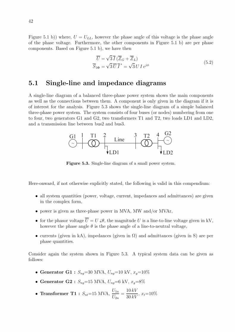
A single-line diagram of a balanced three-phase power system shows the main componentsas well as the connections between them. A component is only given in the diagram if it isof interest for the analysis. Figure 5.3 shows the single-line diagram of a simple balancedthree-phase power system. The system consists of four buses (or nodes) numbering from oneto four, two generators G1 and G2, two transformers T1 and T2, two loads LD1 and LD2,and a transmission line between bus2 and bus3.
~~
1 2 3 4Line
LD1 LD2
G1G2T1 T2
Figure 5.3. Single-line diagram of a small power system.
Here-onward, if not otherwise explicitly stated, the following is valid in this compendium:
• all system quantities (power, voltage, current, impedances and admittances) are givenin the complex form,
• power is given as three-phase power in MVA, MW and/or MVAr,
• for the phasor voltage U = U 6 θ, the magnitude U is a line-to-line voltage given in kV,however the phase angle θ is the phase angle of a line-to-neutral voltage,
• currents (given in kA), impedances (given in Ω) and admittances (given in S) are perphase quantities.
Consider again the system shown in Figure 5.3. A typical system data can be given asfollows:
• Generator G1 : Sng=30 MVA, Ung=10 kV, xg=10%
• Generator G2 : Sng=15 MVA, Ung=6 kV, xg=8%
• Transformer T1 : Snt=15 MVA,U1n
U2n=
10 kV
30 kV, xt=10%
43
• Transformer T2 : Snt=15 MVA,U1n
U2n=
30 kV
6 kV, xt=10%
• Line : r = 0.17 Ω/km, x = 0.3 Ω/km, bc = 3.2× 10⁻⁶ S/km and L = 10 km
• Load LD1 : impedance load, PLD = 15 MW, Un = 30 kV, cosφ = 0.9 inductive
• Load LD2 : impedance load, PLD = 40 MW, Un = 6 kV, cos φ = 0.8 inductive
Comments:
Sng is the generator three-phase rating, Ung is the generator rated (or nominal) line-to-linevoltage and xg is the generator reactance given as a percent based on the generator ratedvalues. The actual value of the generator reactance can be determined by
Xg =xg
100
U2ng
Sng
Ω and Zg = j Xg
In a similar way the actual value of the transformer leakage reactance can be determined,however, depending on which side of the transformer it will be calculated. Having thereactance on the primary side, then it is determined by
Xtp =xt
100
U21n
Snt
Ω and Ztp = j Xtp
Having the reactance on the secondary side, then it is determined by
Xts =xt
100
U22n
SntΩ and Zts = j Xts
For the line, using the model shown in Figure 3.6, we have
Z12 = L (r + jx) Ω and Y sh−12 = jbc L S
For the load, P is the consumed three-phase active power with the power factor cosφ at thenominal (or rated) voltage Un. Thus, the impedance load can be determined by
ZLD =U2n
S∗LD
=U2n
SLD(cosφ− j sinφ)=
U2n
SLD
(cosφ+ j sinφ) where SLD =PLD
cos φ
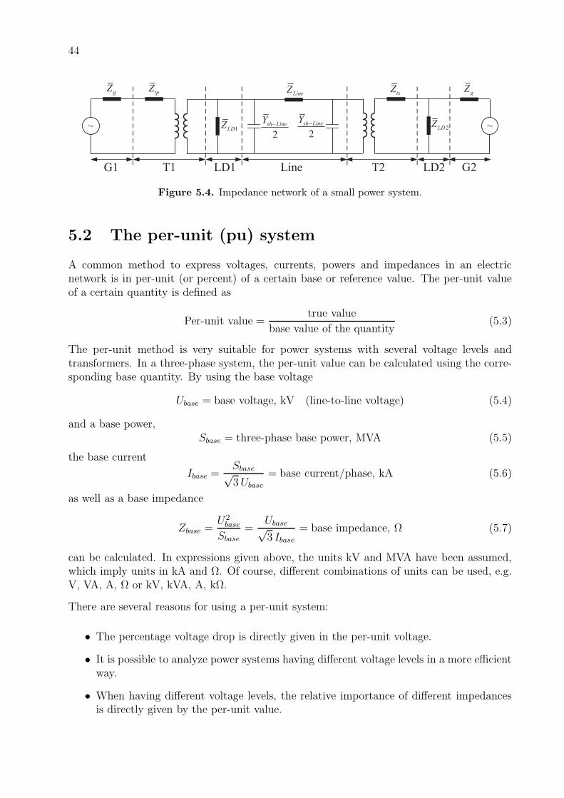
Figure 5.4 shows the single-phase impedance diagram corresponding to the single-line dia-gram shown in Figure 5.3.
The simple system shown in Figure 5.4 has three different voltage levels (6, 10 and 30 kV).The analysis of the system can be carried out by transferring all impedances to a singlevoltage level. This method gives often quite extensive calculations, especially dealing withlarge systems with several different voltage levels. To overcome this difficulty, the so calledper-unit system was developed, and it will be presented in the next section.
44
tpZ
~
gZ
1LDZ
G1 T1 LD1
LineZ
2
sh LineY −
2
sh LineY − ~
gZ
2LDZ
Line T2 LD2
tsZ
G2
Figure 5.4. Impedance network of a small power system.
5.2 The per-unit (pu) system
A common method to express voltages, currents, powers and impedances in an electricnetwork is in per-unit (or percent) of a certain base or reference value. The per-unit valueof a certain quantity is defined as
Per-unit value =true value
base value of the quantity(5.3)
The per-unit method is very suitable for power systems with several voltage levels andtransformers. In a three-phase system, the per-unit value can be calculated using the corre-sponding base quantity. By using the base voltage
Ubase = base voltage, kV (line-to-line voltage) (5.4)
and a base power,Sbase = three-phase base power, MVA (5.5)
the base current
Ibase =Sbase√3Ubase
= base current/phase, kA (5.6)
as well as a base impedance
Zbase =U2base
Sbase
=Ubase√3 Ibase
= base impedance, Ω (5.7)
can be calculated. In expressions given above, the units kV and MVA have been assumed,which imply units in kA and Ω. Of course, different combinations of units can be used, e.g.V, VA, A, Ω or kV, kVA, A, kΩ.
There are several reasons for using a per-unit system:
• The percentage voltage drop is directly given in the per-unit voltage.
• It is possible to analyze power systems having different voltage levels in a more efficientway.
• When having different voltage levels, the relative importance of different impedancesis directly given by the per-unit value.

45
• When having large systems, numerical values of the same magnitude are obtainedwhich increase the numerical accuracy of the analysis.
• Use of the constant√3 is reduced in three-phase calculations.
5.2.1 Per-unit representation of transformers
Figure 5.5 shows the single-phase impedance diagram of a symmetrical three-phase trans-former. In Figure 5.5 a), the transformer leakage impedance is given on the primary side,and in Figure 5.5 b), the transformer leakage impedance is given on the secondary side. Fur-thermore, α is the ratio of rated line-to-line voltages. Thus, based on transformer propertieswe have
U1n
U2n=
1
αand
I1
I2= α (5.8)
Let the base power be Sbase. Note that Sbase is a global base value, i.e. it is the same in alldifferent voltages levels. Let also U1base and U2base be the base voltages on the primary sideand secondary side, respectively. The base voltages have been chosen such that they havethe same ratio as the ratio of the transformer, i.e.
U1base
U2base=
1
α(5.9)
Furthermore, since Sbase =√3U1base I1base =
√3U2base I2base, by virtue of equation (5.9) we
find thatI1baseI2base
= α (5.10)
where, I1base and I2base are the base currents on the primary side and secondary side, respec-tively.
The base impedances on both sides are given by
Z1base =U21base
Sbase=
U1base√3 I1base
and Z2base =U22base
Sbase=
U2base√3 I2base
(5.11)
tpZ
1U 2U
1I 2I1:α
2U
α
tsZ
1U 2U
1I 2I1:α
1Uα
a) b)
Figure 5.5. single-phase impedance diagram of a symmetrical three-phase transformer.

46
Now consider the circuit shown in Figure 5.5 a). The voltage equation is given by
U 1 =√3 I1 Ztp +
U2
α(5.12)
In per-unit (pu), we have
U 1
U1base=
√3 I1 Ztp√
3 I1base Z1base
+U 2
αU1base=
I1I1base
Ztp
Z1base+
U 2
U2base⇒ U1pu = I1pu Ztppu + U 2pu
(5.13)Next, consider the circuit shown in Figure 5.5 b). The voltage equation is given by
αU 1 =√3 I2 Zts + U 2 (5.14)
In per-unit (pu), we have
αU 1
U2base=
αU 1
αU1base=
√3 I2 Zts√
3 I2base Z2base
+U 2
U2base=
I2I2base
Zts
Z2base+
U2
U2base⇒ U 1pu = I2pu Ztspu+U2pu
(5.15)
By virtue of equations (5.13) and (5.15), we find that
I1pu Ztppu = I2pu Ztspu
Furthermore, based on equations (5.8) and (5.10) it can be shown that I1pu = I2pu (showthat). Thus,
Ztppu = Ztspu (5.16)
Equation (5.16) implies that the per-unit impedance diagram of a transformer is the sameregardless of whether the actual impedance is determined on the primary side or on thesecondary side. Based on this property, the single-phase impedance diagram of a three-phasetransformer in per-unit can be drawn as shown in Figure 5.6, where Ztpu = Ztppu = Ztspu.
tpuZ
1puU
puI
2 puU or tpuZpuI1puU 2 puU
Figure 5.6. Per-unit impedance diagram of a transformer.
Example 5.1 Assume that a 15 MVA transformer has a voltage ratio of 6 kV/30 kV anda leakage reactance of 8 %. Calculate the pu-impedance when the base power of the systemis 20 MVA and the base voltage on the 30 kV-side is 33 kV.
Solution
Based on given data, Snt = 15 MVA, U1n/U2n = 6/30, xt = 8% and U2base = 33 kV. We first

47
calculate the transformer impedance in ohm on the 30 kV-side and after that, the per-unitvalue.
Z30kv =Z%
100Ztbase30 =
Z%
100
U22n
Snt
=j8 · 302100 · 15 = j4.8 Ω
Ztpu =Z%
100Ztbase30
Z2base=
Z30kV
Z2base=
Z30kV · Sbase
U22base
=j4.8 · 20
332= j0.088 pu
The given leakage reactance in percent can be considered as the per unit value of reactancebased on the transformer ratings, i.e. Ztbase. To convert this per unit value to the systemper unit value, we may apply the following equation
Ztpu−new = Ztpu−given
U2base−given
Sbase−given
Sbase−new
U2base−new
In our case, Ztpu−given = j 8/100, Ubase−given = U2n = 30, Sbase−given = Snt = 15, Sbase−new =20, and Ubase−new = 33.
Thus,
Ztpu−new =j8
100
302
15
20
332= j0.088 pu (5.17)
The pu-value of the reactance can be also determined based on the base values on the primaryside. From equation (5.9), we have
U1base
U2base=
1
α=
6
30⇒ U1base =
6
30U2base =
6
3033
Z1base =U21base
Sbase
=
(1
α
)2U22base
Sbase
=
(1
α
)2
Z2base
Thus,
Z6kv =Z%
100Ztbase6 =
Z%
100
U21n
Snt=
j8
100
62
15
Ztpu =Z6kV
Z1base=
j8
100
62
15
(30
6
)220
332=
j8
100
302
15
20
332= j0.088 pu
5.2.2 Per-unit representation of transmission lines
Figure 5.7 shows the π-equivalent model of a line, where ysh−kj = Y sh−kj/2.
The voltage at bus k in kV is given by
Uk =√3Zkj I + U j , where I = Ik − Ish = Ik − ysh−kj
Uk√3
Let Sbase, Ubase, Ibase and Zbase be the base values for the line. Note that the base admittanceis given by Ybase = 1/Zbase. Then, the above equations i per unit are given by
Uk
Ubase=
√3Zkj I√
3Zbase Ibase+
U j
Ubase⇒ Ukpu = Zkjpu Ipu + U jpu

48
kUkI
kj kj kjZ R jX= +
jU
2
sh kjY −
2
sh kjY −
shI
I
or
kUkI
kj kj kjZ R jX= +
jU
sh kjy −
shI
I
sh kjy −
Figure 5.7. π-equivalent model of a line.
where
Ipu =IkIbase
− ysh−kj
Uk√3
√3Zbase
Ubase= Ikpu − ysh−kj Zbase
Uk
Ubase= Ikpu − ysh−kjpuUkpu
Figure 5.8 shows the per-unit impedance diagram of a transmission line.
kpuUkjpuZ jpuU
sh kjpuy − sh kjpuy −
Figure 5.8. Per-unit impedance diagram of a transmission line.
5.2.3 System analysis in the per-unit system
To analyze a three-phase power system, it is more convenient and effective to convert thephysical quantities into the per-unit system as follows:
1. Choose a suitable base power for the system. It should be in the same range as therated power of the installed system equipments.
2. Choose a base voltage at one section (or voltage level) of the system. The system isdivided into different sections (or voltage levels) by the transformers.
3. Calculate the base voltages in all sections of the system by using the transformer ratios.
4. Calculate all per-unit values of all system components that are connected.
5. Draw the per-unit impedance diagram of the system.
6. Perform the system analysis (in the per-unit system).
7. Convert the per-unit results back to the physical values.
Example 5.2 Consider the power system shown in Figure 5.9, where a load is fed by agenerator via a transmission line and two transformers. Based on the given system databelow, calculate the load voltage as well as the active power of the load.

49
~
1 2 3 4Line
LD
G T1 T2
Figure 5.9. Single-line diagram of the system in Example 5.2.
System data:
Generator G : Ug=13.8 kV,
Transformer T1 : Snt=10 MVA,U1n
U2n=
13.8 kV
69 kV, Xtp=1.524 Ω (on 13.8 kV-side),
Transformer T2 : Snt=5 MVA,U1n
U2n=
66 kV
13.2 kV, xt=8%,
Line : x = 0.8 Ω/km and L = 10 kmLoad LD : impedance load, PLD = 4 MW, Un = 13.2 kV, cos φ = 0.8 inductive.
Solution
1. Let the base power be Sbase=10 MVA.2. Let the base voltage at the generator be U1base=13.8 kV.3. The transformer ratio gives the base voltage U2base=69 kV for the line andU3base = 69 · 13.2/66 = 13.8 kV for the load.
In Figure 5.10, the different sections of the system are given.
~
1 2 3 4Line
LD
G
1
10 MVA
13.8 kV
base
base
S
U
=
= 2
10 MVA
69 kV
base
base
S
U
=
= 3
10 MVA
13.8 kV
base
base
S
U
=
=
Figure 5.10. Different sections of the system given in Example 5.2.
4. Calculate the per-unit values of the system components.
G: Ugpu = U1pu =Ug
U1base=
13.8
13.8= 1.0 pu
T1: Zt1pu =Ztp
Z1base= j1.524
10
13.82= j0.080 pu
T2: Zt2pu = j8
100
13.22
5
1
Z3base= j
8
100
13.22
5
10
13.82= 0.1464 pu
Line: Z23pu =L z23Z2base
= 10 · j0.8 10
692= j0.0168 pu

50
LD: ZLD =U2n
S∗LD
=U2n
SLD(cosφ− j sinφ)=
U2n
SLD
(cosφ+ j sinφ) =
=13.22
4/0.8(0.8 + j0.6) = 27.8784 + j20.9088 Ω
ZLDpu =ZLD
Z3base
= (27.8784 + j20.9088) · 10
13.82= 1.4639 + j1.0979 pu
5. By using these values, an impedance diagram can be drawn as shown in Figure 5.11.
1 1 0puU = ∠
1t puZ23 puZ
2 puU 3 puU
2t puZ4 puU
LDpuZ
~puI
Figure 5.11. Impedance network in per-unit.
6. The current through the network can be calculated as
Ipu =1 + j0
j0.08 + j0.0168 + j0.1464 + 1.4639 + j1.0979= 0.5037 6 −42.4933 pu (5.18)
The load voltage is
U4pu = ULDpu = Ipu ZLDpu = 0.9217 6 −5.6221 pu (5.19)
The load power isSLDpu = ULDpuI
∗pu = 0.3714 + j0.2785 pu (5.20)
7. The load voltage and active load power in physical units can be obtained by multiplyingthe per-unit values with corresponding base quantities.
ULD = ULDpu U3base = 0.9217 · 13.8 = 12.7199 kV (5.21)
PLD = Real(SLDpu)Sbase = 0.3714 · 10 = 3.714 MW (5.22)
Note that the PLD given in the system data (i.e. PLD=4 MW) is the consumed activepower at the rated (or nominal) voltage Un=13.2 kV. However, the actual voltage at bus 4is 12.7199 kV. Therefore, the actual consumed power is 3.714 MW.
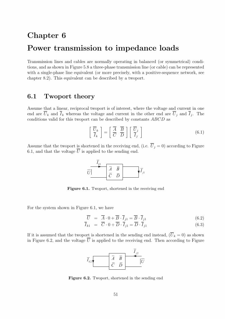
Chapter 6
Power transmission to impedance loads
Transmission lines and cables are normally operating in balanced (or symmetrical) condi-tions, and as shown in Figure 5.8 a three-phase transmission line (or cable) can be representedwith a single-phase line equivalent (or more precisely, with a positive-sequence network, seechapter 8.2). This equivalent can be described by a twoport.
6.1 Twoport theory
Assume that a linear, reciprocal twoport is of interest, where the voltage and current in oneend are Uk and Ik whereas the voltage and current in the other end are U j and Ij . Theconditions valid for this twoport can be described by constants ABCD as
[Uk
Ik
]
=
[A BC D
] [U j
Ij
]
(6.1)
Assume that the twoport is shortened in the receiving end, (i.e. U j = 0) according to Figure6.1, and that the voltage U is applied to the sending end.
UA B
C D
1kI
1jI
Figure 6.1. Twoport, shortened in the receiving end
For the system shown in Figure 6.1, we have
U = A · 0 +B · Ij1 = B · Ij1 (6.2)
Ik1 = C · 0 +D · Ij1 = D · Ij1 (6.3)
If it is assumed that the twoport is shortened in the sending end instead, (Uk = 0) as shownin Figure 6.2, and the voltage U is applied to the receiving end. Then according to Figure
UA B
C D2kI
2jI
Figure 6.2. Twoport, shortened in the sending end
51

52
6.2, we have
0 = A · U − B · Ij2 (6.4)
−Ik2 = C · U −D · Ij2 (6.5)
The reciprocity theorem gives that
Ik2 = Ij1 = I (6.6)
From the equations given above, the following expressions can be derived :
eq. (6.4) ⇒ Ij2 =A
BU (6.7)
eq. (6.7)+(6.6)+(6.2) ⇒ Ij2 = A · I (6.8)
eq. (6.2)+(6.5)+(6.8) ⇒ −I = C · B · I −D ·A · I (6.9)
eq. (6.9), I 6= 0 ⇒ A ·D −B · C = 1 (6.10)
i.e. the determinant of a reciprocal twoport is equal to 1. This implies that if severalreciprocal twoports are connected after one another, the determinant of the total twoportobtained is also equal to 1. With three reciprocal twoports F1, F2 and F3 connected afterone another, the following is always valid :
det(F1F2F3) = det(F1) det(F2) det(F3) = 1 · 1 · 1 = 1 (6.11)
6.1.1 Symmetrical twoports
Assume that a symmetrical linear reciprocal twoport is of interest. If the definitions ofdirections given in Figure 6.3 is used, a current injected in the sending end Ik at the voltage
1UA B
C D
kI 1I
kU
Figure 6.3. Symmetrical twoport, connection 1
Uk gives rise to a current I1 at the voltage U1 in the receiving end. This can be written inan equation as
[Uk
Ik
]
=
[A BC D
] [U 1
I1
]
(6.12)
Suppose that the circuit is fed in the opposite direction, i.e. U1 and I1 are obtained in thesending end according to Figure 6.4. This connection can mathematically be formulated as :
[U 1
−I1
]
=
[A BC D
] [U j
−I j
]
(6.13)

53
1UA B
C D
jI1I
jU
Figure 6.4. Symmetrical twoport, connection 2
By changing the position of the minus sign inside the matrix, equation (6.13) can be rewrittenas [
U 1
I1
]
=
[A −B−C D
] [U j
Ij
]
(6.14)
The matrix in equation (6.14) can be inverted which gives that
[U j
Ij
]
=1
A ·D − B · C︸ ︷︷ ︸
=1
[D BC A
] [U 1
I1
]
(6.15)
Since the twoport is symmetrical, the following is valid
[U j
Ij
]
≡[Uk
Ik
]
(6.16)
The equations (6.12), (6.15) and (6.16) give together that
[A BC D
]
=
[D BC A
]
(6.17)
This concludes that for symmetrical twoports A = D.
6.1.2 Application of twoport theory to transmission line and trans-former and impedance load
Note that all variables in this subsection are expressed in (pu).
Figure 6.5 shows the π-equivalent model of a line.
kUkjZ jU
kI jI
sh kjy − sh kjy −
Figure 6.5. π-equivalent model of a line.

54
From the figure, we have
Uk = U j +(Ij + U j · ysh−kj
)Zkj (6.18)
Ik = Uk · ysh−kj + Ij + U j · ysh−kj
These equations can be rewritten as
Uk =(1 + Zkj · ysh−kj
)U j + Zkj · Ij (6.19)
Ik = ysh−kj
(1 + 1 + Zkj · ysh−kj
)U j +
(Zkj · ysh−kj + 1
)Ij
and by using the matrix notation, this can be written as a twoport equation
[Uk
Ik
]
=
A︷ ︸︸ ︷
1 + ysh−kj · Zkj
B︷︸︸︷
Zkj
ysh−kj(2 + ysh−kj · Zkj)︸ ︷︷ ︸
C
1 + ysh−kj · Zkj︸ ︷︷ ︸
D
[U j
Ij
]
(6.20)
As shown in equation (6.20), a line is symmetrical which gives that A = D. A line is alsoreciprocal which gives that A ·D − B · C = 1.
Using the short line model, then ysh−kj = 0. Therefore, the twoport equation for a short linemodel is given by
[Uk
Ik
]
=
[1 Zkj
0 1
] [U j
Ij
]
(6.21)
The per-unit impedance diagram of a transformer is similar to the per-unit impedance di-agram of a short line. Therefore, the twoport equation for a transformer is similar to thetwoport equation of a short line model, i.e.
[Uk
Ik
]
=
[1 Zt
0 1
] [U j
Ij
]
(6.22)
Figure 6.6 shows the per-unit impedance diagram of an impedance load.
kU
LDZ
jU
kI jI
LDI
Figure 6.6. Impedance diagram of an impedance load.

55
From the figure, the following can be easily obtained.
Uk = U j
Ik = Ij + ILD = Ij +U j
ZLD
(6.23)
Therefore, the twoport equation for an impedance load is given by[Uk
Ik
]
=
[1 01
ZLD1
] [U j
Ij
]
(6.24)
6.1.3 Connection to network
As discussed in section 4.5, based on Thevenin-Helmholtz’s theorem from any output ter-minal in a linear electric network the entire linear electric network as seen from the outputterminal can be modelled as an ideal voltage source UTh in series with an impedance ZTh.Considering any bus in a linear electric network as an output terminal, as seen from any busk the network can be replaced with a Thevenin equivalent as shown in Figure 6.7, whereUk = UTh. Assume that a solid three-phase short circuit (i.e. Zk = 0) is applied to bus k.
ThkZThU
~
k
Figure 6.7. Thevenin equivalent of the network as seen from bus k.
This model implies that the short circuit current is
Isck =UTh kV√3ZThk Ω
kA or Isck =UTh p.u
ZThk p.up.u (6.25)
The question is now how well this model can be adapted to real conditions. For instance,consider the simple system shown in Figure 6.8, where LD is an impedance load and shortline model is used for the lines.
~
A B C DLine1
LD
G T1 T2Line2
E
Figure 6.8. A simple system.
Assume that the initial voltage at bus D is known, i.e. UDi = UDi 6 θDi (p.u). If the pu-valuesof all components are known, then as seen from bus D the following Thevenin equivalent canbe obtained,

56
ThDZThU
~
D
Figure 6.9. Thevenin equivalent seen from bus D.
where,
UTh = UDi and ZThD =Zt1 ZLD
Zt1 + ZLD
+ ZBC + Zt2
If the pu-values of all components are not known, by applying a solid three-phase short circuitto bus D, the short circuit current can be measured and converted to per unit (i.e. Isck (p.u)will be known). Then, the Thevenin impedance as seen from bus D can be calculated as
ZThD =UTh
Isckp.u
Having connected an impedance load ZLDD (p.u) to bus D, the voltage at bus D will be
UD =ZLDD
ZThD + ZLDD
UTh ⇒ UD =
∣∣∣∣
ZLDD
ZThD + ZLDD
∣∣∣∣UTh (6.26)
i.e., the voltage magnitude at bus D will drop with∣∣∣∣
ZLDD
ZThD + ZLDD
∣∣∣∣.100%
Now assume that the transformer T2 has a regulator to automatically regulate the voltagemagnitude at bus D to its initial value, i.e. UDi (p.u). This kind of transformer is known asOn Load Tap Changer (OLTC). When the load is connected to bus D, the OLTC regulatesthe voltage at bus D to UDi, i.e. UD = UDi not the voltage given in equation (6.26). TheThevenin equivalent is not valid in this case. Thevenin-Helmholtz’s theorem is applied tolinear circuits with passive components (static linear circuits), and an OLTC is not a passivecomponent.
Next, as seen from bus E the following Thevenin equivalent can be obtained,
ThEZThU
~
E
Figure 6.10. Thevenin equivalent as seen from bus E.
where, ZThE = ZThD + ZDE and UTh = UEi.
57
Having connected an impedance load ZLDE (p.u) to bus E, the voltage at bus E will be
UE =ZLDE
ZThE + ZLDE
UTh ⇒ UE =
∣∣∣∣
ZLDE
ZThE + ZLDE
∣∣∣∣UTh (6.27)
i.e., the voltage magnitude at bus E will drop with∣∣∣∣
ZLDE
ZThE + ZLDE
∣∣∣∣.100%
If transformer T2 is an OLTC, the voltage at bus D will be recovered to its initial value (i.e.UD = UDi), but not the voltage at bus E. Therefore, the voltage at bus E when the load iconnected will be
UE =
∣∣∣∣
ZLDE
ZDE + ZLDE
∣∣∣∣UDi =
∣∣∣∣
ZLDE
(ZThE − ZThD) + ZLDE
∣∣∣∣UDi (6.28)
The conclusion is that the equivalent impedance from a bus located out in a distributionsystem (with a fairly weak voltage) to the closest bus with regulated voltage can be calculatedas the difference between the Thevenin impedance from the bus with weak voltage and theThevenin impedance from the bus with voltage regulation. To calculate the voltage dropat the connection of the load, the calculated equivalent impedance and the voltage at theregulated bus will be used in the Thevenin equivalent model.
In some cases, the term short circuit capacity Ssck at a bus k is used. It is defined as
Ssck = UThI∗sck = UTh Isck 6 φsck p.u (6.29)
which gives the power that is obtained in the Thevenin impedance. Since this impedanceoften is mostly reactive we have φsck ≈ 90. The short circuit capacity is of interest when theloadability of a certain bus is concerned. The short circuit capacity indicates how much thebus voltage will change for different loading at that bus. The voltage increase at generatorbuses can be also calculated.
Example 6.1 At a bus with a pure inductive short circuit capacity of 500 MVA (i.e. cosφsck =0) an impedance load of 4 MW, cosφLD = 0.8 at nominal voltage, is connected. Calculatethe change in the bus voltage when the load is connected.
Solution
Assume a voltage of 1 pu and a base power Sbase = 500 MVA, i.e. Sscpu = 1 6 90. Thenetwork can then be modeled as shown in Figure 6.11.
The Thevenin impedance can be calculated according to equation (6.25) and (6.29) :
ZThpu =UThpu
Iscpu=
U2Thpu
S∗scpu
=1
1 6 − 90= j1 (6.30)
The load impedance can be calculated as
ZLDpu =U2npu
S∗LDpu
=U2npu
PLD
Sbase·cosφLD
(cosφLD + j sin φLD) =12
4500·0.8
(0.8 + j0.6) (6.31)

58
ThpuZThpuU
~
LDpuZ
LDpuU
Figure 6.11. Single-phase model of system given in the example.
Thus, the voltage ULD at the load is
ULDpu =ZLDpu
ZThpu + ZLDpu
UThpu =80 + j60
j1 + 80 + j601 6 0 = 0.9940 6 − 0.4556 (6.32)
i.e. the voltage drop is about 0.6 %.
Conclusion : A load with an apparent power of 1 % of the short circuit capacity at the busconnected, will cause a voltage drop at that bus of ≈ 1 %.
Example 6.2 As shown in Figure 6.12, a small industry (LD) is fed by a power system viaa transformer (5 MVA, 70/10, x = 4 %) which is located at a distance of 5 km. The electricpower demand of the industry is 400 kW at cosφ=0.8, lagging, at a voltage of 10 kV. Theindustry can be modeled as an impedance load. The 10 kV line has an series impedance of0.9+j0.3 Ω/km and a shunt admittance of j3× 10−6 S/km. Assume that the line is modeledby the π-equivalent. When the transformer is disconnected from bus 3, the voltage at thisbus is 70 kV, and a three-phase short circuit applied to this bus results in a pure inductiveshort circuit current of 0.3 kA.
Calculate the voltage at the industry as well as the power fed by the transformer into theline.
123Line
LD
TPower
system70/10 5 km
Figure 6.12. Single-line diagram of the system in Example 6.2.
Solution
Choose the base values (MVA, kV, ⇒ kA, Ω) :
Sbase = 0.5 MVA, Ubase10 = 10 kV ⇒ Ibase10 = Sbase/√3Ubase10 = 0.0289 kA, Zbase10 =
U2base10/Sbase = 200 Ω

59
Ubase70 = 70 kV ⇒ Ibase70 = Sbase/√3Ubase70 = 0.0041 kA
Calculate the per-unit values of the Thevenin equivalent of the system:
UThpu =UTh
Ubase70=
70 6 0
70= 1 6 0 = 1 and Iscpu =
IscIbase70
=0.3 6 − 90
0.00412= 72.8155 6 − 90
ZThpu =UThpu
Iscpu= j0.0137
Calculate the per-unit values of the transformer:
Ztpu =Zt%
100
Ztbase10
Zbase10=
Zt%
100
U22n
Snt
Sbase
U2base10
=j4
100
102
5
0.5
102=
j4
100
0.5
5= j0.004
Calculate the per-unit values of the line:
Z21pu =5 · (0.9 + j0.3)
Zbase10= 0.0225 + j0.0075
ysh−21pu =Y sh−21pu
2=
5 · (j3× 10−6)
2Zbase10 =
j0.003
2AL = 1 + ysh−21pu · Z21pu = 1.0000 + j0.0000
BL = Z21pu = 0.0225 + j0.0075
CL = ysh−21pu(2 + ysh−21pu · Z21pu) = 0.0000 + j0.0030
DL = AL = 1.0000 + j0.0000
Calculate the per-unit values of the industry impedance:
ZLDpu =U2n
S∗LD
1
Zbase10=
102
0.40.8
(0.8 + j0.6)1
200= 0.8 + j0.6
Figure 6.13 shows the per-unit impedance diagram of the entire system, where the powersystem has been modelled by its Thevenin equivalent. Bus 4 (the terminal bus of the idealvoltage source) is termed as infinite bus.
ThpuZThpuU
~
LDpuZ
21puZtpuZ
123
4
Thévenin equivalent
of the power system
21sh puy − 21sh puy −
Figure 6.13. Per-unit impedance diagram of the system in Example 6.2.
The twoport of the above system (from the infinite bus to bus 1) can be formulated as[UThpu
I4pu
]
=
[1 ZThpu + Ztpu
0 1
] [U2pu
I2pu
]
=
[1 ZThpu + Ztpu
0 1
] [AL BL
CL DL
] [U 1pu
I1pu
]
=
=
[A BC D
] [U 1pu
I1pu
]
=
[0.9999 + j0.0000 0.0225 + j0.02520.0000 + j0.0030 1.0000 + j0.0000
] [U 1pu
I1pu
]

60
As seen from bus 4, the impedance of the entire system (including the industry) can becalculated as
Ztotpu =UThpu
I4pu=
AU 1pu +B I1pu
C U 1pu +D I1pu=
AU1pu
I1pu+B
CU1pu
I1pu+D
=AZLDpu +B
C ZLDpu +D= 0.8254 + j0.6244
⇒ I4pu = UThpu/Ztotpu = 0.9662 6 − 37.1035
The power fed by the transformer into the line can be calculated as[U2pu
I2pu
]
=
[1 ZThpu + Ztrapu
0 1
]−1 [UThpu
I4pu
]
=
[0.9898 6 − 0.7917
0.9662 6 − 37.1035
]
⇒ S2 = U 2pu I∗2pu Sbase = 0.3853 + j0.2832 MVA
the voltage at the industry can be calculated as[U 1pu
I1pu
]
=
[A BC D
]−1 [UThpu
I4pu
]
=
[0.9680 6 − 0.3733
0.9680 6 − 37.2432
]
⇒ U1 (kV) = U1pu Ubase10 = 9.6796 kV
6.2 A general method for analysis of linear balanced
three-phase systems
When analyzing large power systems, it is necessary to perform the analysis in a systematicmanner. Below, a small system is analyzed with a method which can be used for largesystems. In Figure 6.14, an impedance load ZLD1 is fed from an infinite bus (i.e. bus 3
~
1LDZ
21ZtZ123
3I
2I 1I
Figure 6.14. Per unit impedance diagram of a balanced power system.
which is the terminal bus of the ideal voltage source) via a transformer with impedance Zt
and a line with impedance Z21. The voltage at the infinite bus is U 3. All variables areexpressed in per unit. The Y-bus matrix for this system can be formulated as
I1I2I3
= I = YU =
1ZLD1
+ 1Z21
− 1Z21
0
− 1Z21
1Z21
+ 1Zt
− 1Zt
0 − 1Zt
1Zt
U 1
U 2
U 3
(6.33)
The Y-bus matrix can be inverted which results in the corresponding Z-bus matrix :
U = Y−1I = ZI (6.34)

61
Since I1 = I2 = 0, the third row in equation (6.34) can be written as
U3 = Z(3, 3) · I3 ⇒ I3 =U 3
Z(3, 3)(6.35)
where Z(3, 3) is an element in the Z-bus matrix. With that value of the current inserted intoequation (6.34), all system voltages are obtained.
U 1 = Z(1, 3) · I3 (6.36)
U 2 = Z(2, 3) · I3Corresponding calculations can be performed for arbitrarily large systems containing impedanceloads and one voltage source.
a) ~
1LDZ
21ZtZ123
2LDI ′
2LDZ
b) ~
1LDZ
21ZtZ123
2 0LDI =
2LDZ
~2U
c)
1LDZ
21ZtZ12
2LDZ
~2U−
2 2LDI I∆′= −
1 0I∆ =
U′
preU
U∆
Figure 6.15. Total voltage obtained by using superposition
Assume that an impedance ZLD2 is added to the system at bus 2, as shown in Figure 6.15a). This will change the voltage magnitudes at all buses with exception of the bus connectedto the voltage source (bus 3 in this example). Then, the actual voltages can be expressed by
U′ = Upre +U∆ (6.37)
where U′ is a vector containing the actual voltages due to the change, Upre is a vectorcontaining the voltages of all buses (with exception of the bus connected to the voltage

62
source) prior to the change and U∆ is the applied change. This equation can be illustratedgraphically as shown in Figure 6.15, i.e. the total voltage can be calculated as a superpositionof two systems with equal impedances but with different voltage sources.
As indicated by the system in Figure 6.15 c), the feeding voltage is −U 2 while the voltagesource at bus 3 is shortened (when the voltage source is short circuited the bus connectedto the voltage source (i.e. bus 3) is removed). The Y-bus matrix for this system can beobtained by removing the row and column corresponding to bus 3 in Y (see equation (6.33))since bus 3 is grounded and removed. If bus 3 was kept in the mathematical formulation,Y(3, 3) = ∞ since the impedance to ground is zero.
[I∆1
I∆2
]
= I∆ = Y∆U∆ =
[1
ZLD1+ 1
Z21− 1
Z21
− 1Z21
1Z21
+ 1Zt
][U∆1
U∆2
]
(6.38)
The expression given above, can be inverted which gives the corresponding Z-bus matrix :
U∆ = Y−1∆ I∆ = Z∆I∆ ⇒
[U∆1
U∆2
]
=
[Z∆(1, 1) Z∆(1, 2)Z∆(2, 1) Z∆(2, 2)
] [I∆1
I∆2
]
(6.39)
In this equation, I∆1 = 0 which is shown in Figure 6.15 c). This gives that the second rowcan be written as
U∆2 = Z∆(2, 2)I∆2 (6.40)
Figure 6.14 gives the same currents as Figure 6.15 b), since the voltage over ZLD2 in Figure
6.15 b) is zero. This implies that the current through ZLD2 is zero. Therefore, I∆2 = −I′LD2.
At bus 2 in Figure 6.15 a) the following is valid
U′2 = I
′LD2 · ZLD2 = −I∆2 · ZLD2 (6.41)
By combining equations (6.37), (6.40) and (6.41), the following can be obtained
I∆2 =−U 2
ZLD2 + Z∆(2, 2)(6.42)
By inserting that value in the equations given above, all voltages after the system changecan be calculated as :
U′2 =
ZLD2
ZLD2 + Z∆(2, 2)U 2 (6.43)
U′1 = U1 −
Z∆(1, 2)
ZLD2 + Z∆(2, 2)U 2 (6.44)
The procedure given above can be generalized to be used for an arbitrarily large system.Assume that an impedance Zr is connected to a bus r and an arbitrary bus is termed i. Thecurrent I
′r (=−I∆r) through Zr can be calculated as well as the voltages after connection of
the impedance Zr at bus r. The equations are as follows.
I′r =
U r
Zr + Z∆(r, r)(6.45)
U′r =
Zr
Zr + Z∆(r, r)U r (6.46)
U′i = U i −
Z∆(i, r)
Zr + Z∆(r, r)U r (6.47)

63
Note that i 6= r, and bus r and bus i do not represent the bus connected to the voltagesource.
The Thevenin equivalent at a bus in a symmetrical network can be calculated by usingequations (6.37) and (6.39). At bus r (r=2 in this case), the equation will be as
U′(r) = Upre(r) + Z∆(r, r)I∆(r) (6.48)
where
Upre(r) = UThr Thevenin voltage at bus r prior to the change, see Figure 6.16.
Z∆(r, r) = ZThr Thevenin impedance as seen from bus r, see Figure 6.16.
I∆(r) = −I′r The actual injected current into bus r.
U′(r) = U′r the actual voltage at bus r.
( , )Z r r∆
preU ( )r
~
r
U ( )r′I ( )r∆
ThrZThrU
~
r
rU ′
rI ′
or
Figure 6.16. Thevenin equivalent at bus r in a symmetrical three-phase network.
As given by equation (6.48) and Figure 6.16, U′(r) = Upre(r) if I∆(r) = 0. This formu-lation shows that the Thevenin voltage at bus r can be calculated as the voltage at bus rwhen the bus is not loaded, i.e. I∆(r) = 0. The Thevenin impedance is found as the r-thdiagonal element of the impedance matrix Z∆ which is determined when the voltage sourceis shortened.
Example 6.3 In Figure 6.17, an internal network of an industry is given. Power is deliveredby an infinite bus with a nominal voltage at bus 1. Power is transmitted via transformer T1,Line2 and transformer T2 to the load LD2. There is also a high voltage load LD1 connected
1
2 3
4
Line1
LD1T1
T2Line2
5
LD2
Figure 6.17. Single-line diagram of an internal industry network
to T1 via Line1. The system data is given as follows:

64
• Transformer T1 : 800 kVA, 70/10, x = 7 %
• Transformer T2 : 300 kVA, 10/0.4, x = 8 %
• Line1 : r = 0.17 Ω/km, x = 0.3Ω/km, bc = 3.2× 10⁻⁶ S/km, L = 2 km
• Line2 : r = 0.17 Ω/km, x = 0.3Ω/km, bc = 3.2× 10⁻⁶ S/km, L = 1 km
• Load LD1 : impedance load, 500 kW, cosφ = 0.80, inductive at 10 kV
• Load LD2 : impedance load, 200 kW, cosφ = 0.95, inductive at 0.4 kV
The π-equivalent model is used for the lines.
Calculate the efficiency of the internal network as well as the short circuit current that isobtained at a solid three-phase short circuit at bus 4.
Solution
1
2 3
4 5
1t puZ
23 puZ
23sh puy − 1LD puZ
24 puZ
2LD puZ
2t puZ
24sh puy −
Figure 6.18. Network in Example 6.3.
Choose the base values (MVA, kV, ⇒ kA, Ω) :Sbase = 500 kVA = 0.5 MVA, Ubase70 = 70 kV
Ubase10 = 10 kV ⇒ Ibase10 = Sbase/√3Ubase10 = 0.0289 kA, Zbase10 = U2
base10/Sbase = 200 Ω
Ubase04 = 0.4 kV ⇒ Ibase04 = Sbase/√3Ubase04 = 0.7217 kA, Zbase04 = U2
base04/Sbase = 0.32 Ω
Calculate the per-unit values of the infinite bus :U 1 = 70/Ubase70 = 70/70 = 1
Calculate the per-unit values of the transformer T1 :Zt1pu = (Zt1%/100) ·Zt1base10/Zbase10 = (ZT1%/100) ·Sbase/Snt1 = (j7/100) ·0.5/0.8 = j0.0438
Calculate the per-unit values of the transformer T2 :Zt2pu = (Zt2%/100) · Sbase/Snt2 = (j8/100) · 0.5/0.3 = j0.1333
Calculate the per-unit values of Line1 :

65
Z23pu = L(r + jx)/Zbase10 = 2 · (0.17 + j0.3)/Zbase10 = 0.0017 + j0.003ysh−23pu = jL bc Zbase10/2 = j2 · (3.2× 10−6) · Zbase10/2 = j0.0013/2
Calculate the per-unit values of Line2 :Z24pu = L(r + jx)/Zbase10 = 1 · (0.17 + j0.3)/Zbase10 = 0.0009 + j0.0015
ysh−24pu = jL bc Zbase10/2 = j1 · (3.2× 10−6) · Zbase10/2 = j0.00064/2Calculate the per-unit values of the impedance LD1 :ZLD1pu = (U2
LD1/S∗LD1)/Zbase10 = (102/[0.5/0.8]) · (0.8 + j0.6)/200 = 0.64 + j0.48
Calculate the per-unit values of the impedance LD2 :ZLD2pu = (U2
LD2/S∗LD2)/Zbase04 = (0.42/0.2/0.95) · (0.95 + j
√1− 0.952)/0.32 = 2.2562 +
j0.7416
Calculate the Y-bus matrix of the network. The grounding point is not included in the Y-busmatrix since the system then is overdetermined.
Y =
1Zt1pu
− 1Zt1pu
0 0 0
− 1Zt1pu
Y 22 − 1Z23pu
− 1Z24pu
0
0 − 1Z23pu
Y 33 0 0
0 − 1Z24pu
0 Y 44 − 1Zt2pu
0 0 0 − 1Zt2pu
1Zt2pu
+ 1ZLD2pu
(6.49)
where
Y 22 =1
Zt1pu
+1
Z23pu
+ ysh−23pu +1
Z24pu
+ ysh−24pu
Y 33 =1
Z23pu
+ ysh−23pu +1
ZLD1pu
Y 44 =1
Z24pu
+ ysh−24pu +1
Zt2pu
Next, we haveI = YU (6.50)
which can be rewritten as
U 1
U 2
U 3
U 4
U 5
= U = Y−1I = ZI = Z
I1I2I3I4I5
(6.51)
The Z-bus matrix can be calculated by inverting the Y-bus matrix :
Z =
0.510+j0.375 0.510+j0.331 0.508+j0.329 0.510+j0.331 0.516+j0.298
0.510+j0.331 0.510+j0.331 0.508+j0.329 0.510+j0.331 0.516+j0.298
0.508+j0.329 0.508+j0.329 0.509+j0.330 0.508+j0.329 0.515+j0.296
0.510+j0.331 0.510+j0.331 0.508+j0.329 0.510+j0.332 0.517+j0.299
0.516+j0.298 0.516+j0.298 0.515+j0.296 0.517+j0.299 0.529+j0.397
(6.52)

66
Since all injected currents with exception of I1 are zero, I1 can be calculated using the firstrow in equation (6.51) :
U 1 = Z(1, 1)I1 ⇒ I1 = U1/Z(1, 1) = 1.0/(0.510 + j0.375) = 1.58 6 − 36.33 (6.53)
The voltages at the other buses can be easily be solved by using equation (6.51) :
U 2 = Z(2, 1)I1 = (0.510 + j0.331) · (1.58 6 − 36.33) = 0.9606 6 − 3.324
U 3 = Z(3, 1)I1 = (0.508 + j0.329) · (1.58 6 − 36.33) = 0.9569 6 − 3.423 (6.54)
U 4 = Z(4, 1)I1 = (0.510 + j0.331) · (1.58 6 − 36.33) = 0.9601 6 − 3.350
U 5 = Z(5, 1)I1 = (0.516 + j0.298) · (1.58 6 − 36.33) = 0.9423 6 − 6.351
The total amount of power delivered to the industry is
S1 = U 1 · I∗1 · Sbase = 0.6367 + j0.4682 MVA (6.55)
The power losses in Line1 and Line2 can be calculated as
IZ23 =(U2 − U 3)/Z23pu = 1.1957 6 − 40.27
IZ24 =(U2 − U 4)/Z24pu = 0.3966 6 − 24.50
PfLine1 =Real(Z23pu)I2Z23 · Sbase = 0.0012 MW
PfLine2 =Real(Z24pu)I2Z24 · Sbase = 0.0000669MW
(6.56)
The efficiency for the network is then
η =Real(S1)− PfLine1 − PfLine2
Real(S1)= 0.9980 ⇒ 99.80% (6.57)
A solid short circuit at bus 4 can be calculated by connecting an impedance with Z4 = 0 atbus 4. According to section 6.2, the current through the impedance Z4 can be determined byremoving the row and the column of the Y-bus matrix that corresponds to the bus connectedto the voltage source (i.e. bus 1 in this example). Thus,
Y∆ = Y(2 : 5, 2 : 5) =
Y 22 − 1Z23pu
− 1Z24pu
0
− 1Z23pu
Y 33 0 0
− 1Z24pu
0 Y 44 − 1Zt2pu
0 0 − 1Zt2pu
1Zt2pu
+ 1ZLD2pu
(6.58)
The inverse of this matrix is
Z∆ = Y−1∆ =
0.0024+j0.0420 0.0025+j0.0418 0.0025+j0.0419 0.0046+j0.0410
0.0025+j0.0418 0.0043+j0.0446 0.0025+j0.0418 0.0046+j0.0408
0.0025+j0.0419 0.0025+j0.0418 0.0033+j0.0434 0.0055+j0.0424
0.0046+j0.0410 0.0046+j0.0408 0.0055+j0.0424 0.0144+j0.1719
(6.59)
The short circuit current at bus 4 can then be calculated according to equation (6.45).
Isc4 =U 4
Z4 + Z∆(4, 4)︸ ︷︷ ︸
element (3,3) in Z∆
Ibase10 =0.9601 6 − 3.350
0 + (0.0033 + j0.0434)0.0289 =
= 0.6366 6 − 88.97 kA (6.60)

67
6.3 Extended method to be used for power loads
The method described in section 6.2 is valid when all system loads are modeled as impedanceloads, i.e. the power consumed is proportional to the voltage squared. In steady-stateconditions, an often used load model is the constant power model. The method describedin section 6.2 can be used in an iterative way, described as follows:
1. Calculate the per-unit values of all components that are of interest. Loads that aremodeled with constant power (independent of the voltage) are replaced by impedances.The impedance of a load at bus k can be calculated as ZLDk = U2
n/S∗LDk where Un = 1
pu is the rated (or nominal) voltage, and SLDk is the rated power of the load.
2. Calculate the Y-bus matrix and the corresponding Z-bus matrix of the network as wellas the load impedances. By using the method described in section 6.2 (equation (6.35)and (6.36)), the voltage at all buses can be calculated.
3. Calculate the load demand at all loads. The power demand SLDk−b at load LDk isobtained as SLDk−b = U2
k/Z∗LDk where Uk is the actual calculated voltage at bus k.
4. Calculate the difference between the actual calculated and specified load demand forall power loads :
∆PLDk = |Re(SLDk−b)− Re(SLDk)| (6.61)
∆QLDk = |Im(SLDk−b)− Im(SLDk)| (6.62)
5. If ∆PLDk and/or ∆QLDk are too large for a certain bus :
(a) Calculate new load impedances according to ZLDk = U2k/S
∗LDk where Uk is the
actual calculated voltage at bus k obtained in step 3,
(b) Go back to step 2 and repeat the calculations.
If ∆PLDk and ∆QLDk are found to be acceptable for all power loads, the iterationprocess is finished.
A simple example will be given to clarify this method.
Example 6.4 Assume a line operating with a voltage of U1 = 225 6 0 kV in the sendingend, i.e. bus 1, and with a load of PLD = 80 MW and QLD = 60 MVAr in the receiving end,i.e. bus 2. The line has a length of 100 km with x = 0.4 Ω/km, r = 0.04 Ω/km and bc =3× 10⁻⁶ S/km. Calculate the receiving end voltage.
Solution
In Figure 6.19, the network modeled by impedance loads is given.
Assume Sbase = 100 MVA and Ubase = 225 kV which gives
Zbase = U2base/Sbase = 506.25 Ω

68
1 212Z
12 12sh shy jb− −= LD LD LDS P jQ= +
12I
Figure 6.19. Impedance diagram of the system in Example 6.4.
This gives the following per-unit values of the line
U1pu = 225/Ubase = 1.0, PLDpu = PLD/Sbase = 0.8, QLDpu = QLD/Sbase = 0.6
Z12pu = L (r + j x)/Zbase = 100 (0.04 + j 0.4)/Zbase = 0.0079 + j 0.0790
Based on equation (3.9),bsh−12pu = L bc Zbase/2 = 100 (3× 10⁻⁶)Zbase/2 = 0.0759
The iteration process can now be started :
1. U2pu = 1, ZLDpu = U22pu/(PLDpu − jQLDpu) = 0.8 + j0.6
2. I12pu = U1pu/(Z12pu +1
jbsh−12pu‖ ZLDpu) = 0.7330 - j0.5415 ⇒ U2pu = |U1pu − I12puZ12pu|
= 0.9529
3. SLDpu = U22pu/Z
∗LDpu = 0.7265 + j0.5448
4. ∆PLD = 0.0735, ∆QLD = 0.0552
1. ZLDpu = 0.7265 + j0.5448
2. U2pu = 0.9477
4. ∆PLD = 0.0087, ∆QLD = 0.0066
1. ZLDpu = 0.7185 + j0.5389
2. U2pu = 0.9471
4. ∆PLD = 0.0011, ∆QLD = 0.00079
1. ZLDpu = 0.7176 + 0.5382i
2. U2pu = 0.9470
4. ∆PLD = 0.0001, ∆QLD = 0.0001
This is found to be acceptable, which gives a voltage magnitude in the sending end ofU2 = 0.9470 · Ubase = 213.08 kV. This simple example can be solved exactly by using anon-linear expression which will be shown in Example 7.4.
Example 6.5 Consider the system in Example 6.2, but let the short line model be used forthe line (i.e. bc = 0), and the load be considered as a constant power load.
Calculate the voltage level at the industry.
Solution
1. From Example 6.2, we have the following:
UThpu = 1, ZThpu = j0.0137, Ztpu = j0.004, Z21pu = 0.0225 + j0.0075

69
totpuZThpuU
LD LD LDS P jQ= +
LDpuU
Figure 6.20. Network used in Example 6.5.
The total impedance between bus 1 and bus 4 is given by:
Ztotpu = ZThpu + Ztpu + Z21pu = 0.0225 + j0.0252
Calculate the per-unit values of the power demand of the industry as well as the correspond-ing impedance at nominal voltage :SLDpu = (PLD + j[PLD/ cosφ] · sinφ)/Sbase = 0.8000 + j0.6000
ZLDpu = (U2n/S
∗LDpu)/U
2base10 = 0.8 + j0.6
2. The Y-bus matrix of the network can be calculated as :
Y =
[1
Ztotpu− 1
Ztotpu
− 1Ztotpu
1Ztotpu
+ 1ZLDpu
]
=
[19.67− j22.08 −19.67 + j22.08−19.67 + j22.08 20.47− j22.68
]
(6.63)
The Z-bus matrix is calculated as the inverse of the Y-bus matrix :
Z = Y−1 =
[0.82 + j0.63 0.80 + j0.600.80 + j0.60 0.80 + j0.60
]
(6.64)
The voltage at the industry is now calculated according to equation (6.36) :
ULDpu = Z(2, 1) · UThpu/Z(1, 1) = 0.9679 6 − 0.3714 (6.65)
3. The power delivered to the industry can be calculated as :
SLDpu−b = U2LD/Z
∗LDpu = 0.7495 + j0.5621 (6.66)
4. The difference between calculated and specified power can be calculated as :
∆PLD = |Re(SLDpu−b)−Re(SLDpu)| = 0.0505 (6.67)
∆QLD = |Im(SLDpu−b)− Im(SLDpu)| = 0.0379 (6.68)
5. These deviations are too large and the calculations are therefore repeated and a newindustry impedance is calculated by using the new voltage magnitude :
ZLDpu = (U2LDpu/S
∗LDpu) = 0.7495 + j0.5621 (6.69)
Repeat the calculations from step 2.
2, 3. ⇒ SLDpu−b = 0.7965 + j0.59744. ∆PLD = 0.0035, ∆QLD = 0.0026
70
Unacceptable ⇒5. ZLDpu = 0.7462 + j0.5597Continue from step 2.
2, 3. ⇒ SLDpu−b = 0.7998 + j0.59984. ∆PLD = 0.00024, ∆QLD = 0.00018Unacceptable ⇒5. ZLDpu = 0.7460 + j0.5595Continue from step 2.
2, 3. ⇒ SLDpu−b = 0.8000 + j0.60004. ∆PLD = 0.000016, ∆QLD = 0.000012Acceptable ⇒ULD = ULDpu · Ubase10 = 9.6565 6 − 0.3974

Chapter 7
Power flow calculations
In chapters 5 and 6, it was assumed that the network had only one voltage source (orgenerator bus), and the loads were modelled as impedances. These assumptions resulted inusing a linear set of equations which could be easily solved.
In this chapter, the loads are modelled as constant power loads, and the system has morethan one generator bus (i.e. a multi-generator system).
First, the power flow in a transmission line will be derived, and then a more general powerflow calculations (commonly known as load flow) will be presented.
7.1 Power flow in a line
Consider the the π-equivalent model of a line shown in Figure 7.1, where all variables ex-pressed in per-unit.
kjZ
sh kjjb −
IkU jU
sh kjjb −
shI
kjS
Figure 7.1. π-equivalent model of a line.
Let
Uk = Ukejθk , U j = Uje
jθj
Zkj = Rkj + jXkj , Zkj =√
R2kj +X2
kj
θkj = θk − θj
(7.1)
The power Skj in the sending end k is given by
Skj = Uk
(
I∗sh + I
∗)
= Uk
(
(j bsh−kj Uk
)∗+
U∗k − U
∗j
Z∗kj
)
=
= −j bsh−kj U2k +
U2k
Rkj − jXkj
− UkUj
Rkj − jXkj
ej(θk−θj) =
= −j bsh−kj U2k +
U2k
Z2kj
(Rkj + jXkj)−UkUj
Z2kj
(Rkj + jXkj) (cos θkj + j sin θkj)
(7.2)
71

72
By dividing equation (7.2) into a real and an imaginary part, expressions for the active andreactive power can be obtained, respectively, as
Pkj =Rkj
Z2kj
U2k +
Uk Uj
Z2kj
(Xkj sin θkj − Rkj cos θkj)
=Rkj
Z2kj
U2k +
Uk Uj
Zkjsin
(
θkj − arctan
(Rkj
Xkj
)) (7.3)
Qkj = −bsh−kj U2k +
Xkj
Z2kj
U2k − UkUj
Z2kj
(R sin θkj +Xkj cos θkj)
=
(
−bsh−kj +Xkj
Z2kj
)
U2k − Uk Uj
Zkj
cos
(
θkj − arctan
(Rkj
Xkj
)) (7.4)
From equations (7.3) and (7.4), it can be concluded that if the phasor voltages (i.e. thevoltage magnitude and phase angle) at both ends of the line are known, the power flow canbe uniquely determined. This implies that if the phasor voltages of all buses in a system areknown, the power flows in the whole system are known, i.e the phasor voltages define thesystem state.
Example 7.1 Assume a line where the voltage in the sending end is U 1 = 225 6 0 kV andin the receiving end U2 = 213.08 6 − 3.572 kV. The line has a length of 100 km and hasx = 0.4 Ω/km, r = 0.04 Ω/km and bc = 3 × 10⁻⁶ S/km. Calculate the amount of powertransmitted from bus 1 to bus 2.
Solution
Assume Sbase = 100 MVA and Ubase = 225 kV, this gives that
Zbase = U2base/Sbase = 506.25 Ω
The per-unit values for the line are
U1 = 225/Ubase = 1.0 pu, U2 = 213.08/Ubase = 0.9470 pu, θ12 = 0-(-3.572) = 3.572
R12 = 0.04 · 100/Zbase = 0.0079 pu, X12 = 0.4 · 100/Zbase = 0.0790 pu,
bsh−12 = 3× 10−6 · 100 · Zbase/2 = 0.0759 pu, Z12 =√
R212 +X2
12 = 0.0794 pu
The power flow in per-unit can be calculated by using equation (7.3) and (7.4) :
P12 =0.0079
0.079421.02 +
1.0 · 0.94700.0794
sin
(
3.572 − arctan
(0.0079
0.0790
))
=
= 0.8081 pu
Q12 =
(
−0.0759 +0.0790
0.07942
)
∗ 1.02 − 1.0 · 0.94700.0794
cos
(
3.572 − arctan
(0.0079
0.0790
))
=
= 0.5373 pu
expressed in nominal values
P12 = 0.8081 · Sbase = 80.81 MW
Q12 = 0.5373 · Sbase = 53.73 MVAr

73
For this simple system, the calculations can be performed without using the per-unit system.By using equation (5.7), equation (7.3) can be rewritten as
Pkj(MW) = Pkj(pu)Sbase =U2base
Zbase
Rkj
Z2kj
U2k +
Uk Uj
Zkjsin
(
θkj − arctan
(Rkj
Xkj
))
=
=Rkj(Ω)
Z2kj(Ω)
U2k (kV) +
Uk(kV) · Uj(kV)
Zkj(Ω)sin
(
θkj − arctan
(Rkj
Xkj
))
i.e. this equation is the same independent on if the values are given as nominal or per-unitvalues. Note that arctan(Rkj/Xkj) = arctan(Rkj(Ω)/Xkj(Ω)).
For a high voltage overhead line (U > 70 kV), the line reactance is normally considerablyhigher than the resistance of the line, i.e. Rkj ≪ Xkj in equation (7.3). An approximateform of that equation is (i.e. Rkj ≈ 0)
Pkj ≈UkUj
Xkjsin θkj (7.5)
i.e. the sign of θkj determines the direction of the active power flow on the line. Normally,the active power will flow towards the bus with the lowest voltage angle. This holds also forlines having a pronounced resistivity.
Assume that the voltages Uk and U j are in phase and that the reactance of the line isdominating the line resistance (i.e. R ≈ 0). This implies that the active power flow is verysmall. Equation (7.4) can be rewritten as
Qkj = −bsh−kj U2k +
Uk(Uk − Uj)
Xkj
(7.6)
Equation (7.6) indicates that this type of line gives a reactive power flow towards the buswith the lowest voltage magnitude. The equation shows that if the difference in voltagemagnitude between the ends of the line is small, the line will generate reactive power. Thissince the reactive power generated by the shunt admittances in that case dominates thereactive power consumed by the series reactance. The “rule of thumb” that reactive powerflows towards the bus with lowest voltage is more vague than the rule that active powerflows towards the bus with lowest angle. The fact that overhead lines and especially cables,generates reactive power when the active power flow is low, is important to be aware of.
Example 7.2 Using the approximate expressions (7.5) and (7.6), respectively, calculate theactive and reactive power flow in the line in Example 7.1.
Solution
P12 ≈ 1.0 · 0.94700.0790
sin 3.572 = 0.7468 pu ⇒ 74.68 MW
Q12 ≈ −0.0759 · 1.02 + 1.0(1.0− 0.9470)
0.0790= 0.5948 pu ⇒ 59.48 MVAr
The answers are of right dimension and have correct direction of the power flow but theactive power flow is about 8 % too low and the reactive power flow is 11 % too large.

74
7.1.1 Line losses
The active power losses on a three-phase line are dependent on the line resistance and theactual line current. By using physical units (i.e. not in per-unit), the losses can be calculatedas
Pf = 3RkjI2 (7.7)
The squared current dependence in equation (7.7) can be written as
I2 = Iej γ Ie−j γ = I I∗=
S∗
√3U
∗S√3U
=S2
3U2=
P 2 +Q2
3U2(7.8)
The active power losses for the line given in Figure 7.1 can be calculated as
Pf = Rkj
P 2kj + (Qkj + bsh−kj U
2k )
2
U2k
(7.9)
where, bsh−kj U2k is the reactive power generated by the shunt capacitance at bus k.
The expression given by (7.9) is valid both for nominal and for per-unit values. This equationshows that a doubling of transmitted active power will increase the active power losses by afactor of four. If the voltage is doubled, the active power losses will decrease with a factorof four.
Assume that the active power injections at both ends of the line are known, i.e. both Pkj
and Pjk have been calculated using equation (7.3). The active power losses can then becalculated as
Pf = Pkj + Pjk (7.10)
The reactive power losses can be obtained in the corresponding manner
Qf = 3XkjI2 = Xkj
P 2kj + (Qkj + bsh−kj U
2k )
2
U2k
(7.11)
Equations (7.8) and (7.9) shows that the losses are proportional to S2 and that the losseswill increase if reactive power is transmitted over the line. A natural solution to that is togenerate the reactive power as close to the consumer as possible. Of course, active poweris also generated as close to the consumer as possible, but the generation costs are of greatimportance.
Example 7.3 Use the same line as in Example 7.1 and calculate the active power losses.
Solution
The losses on the line can be calculated by using equation (7.9) and the conditions thatapply at the sending end
Pf(MW) = R12P 212 + (Q12 + bsh−12U
21 )
2
U21
Sbase =
= 0.00790.80812 + (0.5373 + 0.0759 · 1.02)2
1.02100 = 0.81 MW
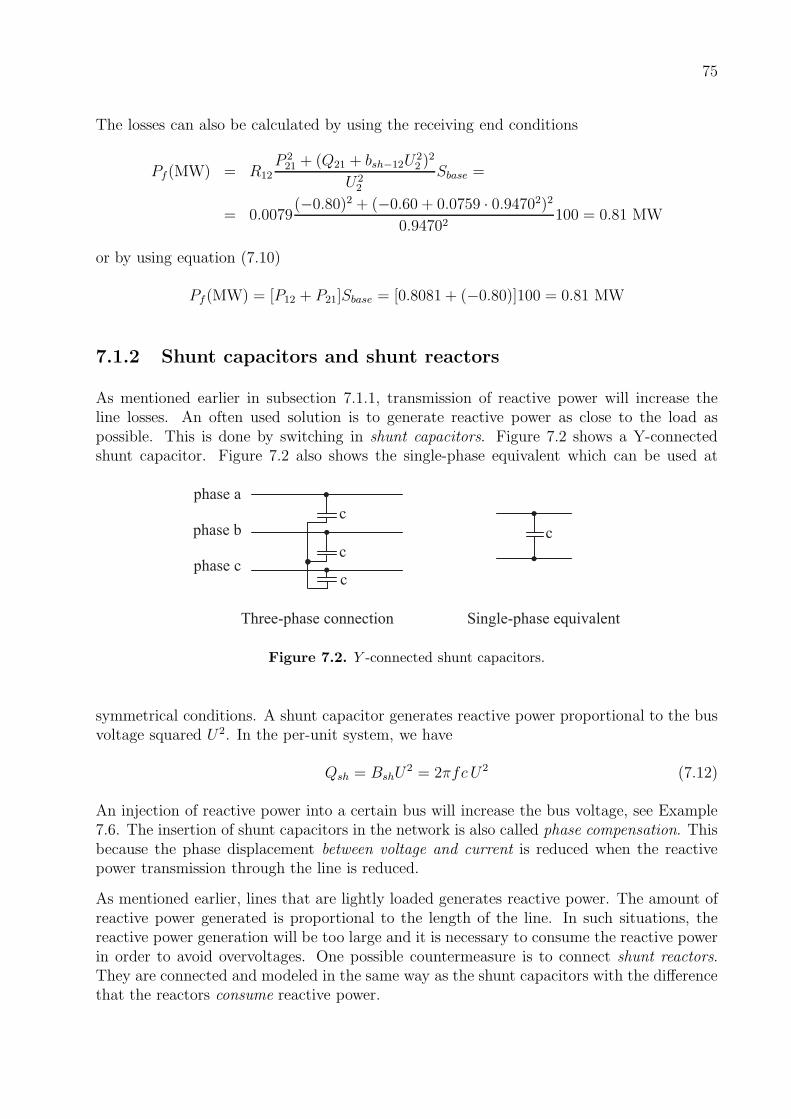
75
The losses can also be calculated by using the receiving end conditions
Pf(MW) = R12P 221 + (Q21 + bsh−12U
22 )
2
U22
Sbase =
= 0.0079(−0.80)2 + (−0.60 + 0.0759 · 0.94702)2
0.94702100 = 0.81 MW
or by using equation (7.10)
Pf(MW) = [P12 + P21]Sbase = [0.8081 + (−0.80)]100 = 0.81 MW
7.1.2 Shunt capacitors and shunt reactors
As mentioned earlier in subsection 7.1.1, transmission of reactive power will increase theline losses. An often used solution is to generate reactive power as close to the load aspossible. This is done by switching in shunt capacitors. Figure 7.2 shows a Y-connectedshunt capacitor. Figure 7.2 also shows the single-phase equivalent which can be used at
phase a
c
Three-phase connection Single-phase equivalent
phase b
phase cc
c
c
Figure 7.2. Y -connected shunt capacitors.
symmetrical conditions. A shunt capacitor generates reactive power proportional to the busvoltage squared U2. In the per-unit system, we have
Qsh = BshU2 = 2πfc U2 (7.12)
An injection of reactive power into a certain bus will increase the bus voltage, see Example7.6. The insertion of shunt capacitors in the network is also called phase compensation. Thisbecause the phase displacement between voltage and current is reduced when the reactivepower transmission through the line is reduced.
As mentioned earlier, lines that are lightly loaded generates reactive power. The amount ofreactive power generated is proportional to the length of the line. In such situations, thereactive power generation will be too large and it is necessary to consume the reactive powerin order to avoid overvoltages. One possible countermeasure is to connect shunt reactors.They are connected and modeled in the same way as the shunt capacitors with the differencethat the reactors consume reactive power.

76
7.1.3 Series capacitors
By studying equation (7.5), an approximate expression of the maximum amount of powerthat can be transmitted through a line, at a certain voltage level, can be written as
Pkj−max ≈ maxθkj
UkUj
Xkjsin θkj =
UkUj
Xkj(7.13)
i.e. the larger the reactance of the line is, the less amount of power can be transmitted.One possibility to increase the maximum loadability of a line is to compensate for the seriesreactance of the line by using series capacitors. In Figure 7.3, the way of connecting seriescapacitors is shown as well as the single-phase equivalent of a series compensated line. The
( )kj kj kj cZ R j X X= + -
sh kjjb- sh kjjb
-
Three-phase connection Single-phase equivalent
phase a
phase b
phase c
c
c
c
Figure 7.3. Series capacitors
expression for the maximum loadability of a series compensated line is
Pkj−max ≈ UkUj
Xkj −Xc
(7.14)
It is obvious that the series compensation increases the loadability of the line.
The use of series capacitors will also reduce the voltage drop along the line, see Example7.7.
7.2 Non-linear power flow equations
The technique of determining all bus voltages in a network is usually called load flow. Whenknowing the voltage magnitude and voltage angle at all buses, the system state is completelydetermined and all system properties of interest can be calculated, e.g. line loadings andline losses.
In a power system, power can be generated and consumed at many different locations. Con-sider now a balanced power system with N buses. Figure 7.4 schematically shows connectionof the system components to bus k.
The generator generates the current IGk (in pu), the load at the bus draws the current ILDk
(in pu), and Ikj (in pu) is the currents from bus k to the neighboring buses. According to

77
GkIkU
~
LDkI
1kI
2kI
kNI
Figure 7.4. Notation of bus k in a network.
Kirchoff’s current law, the sum of all currents injected into bus k must be zero, i.e.
IGk − ILDk =
N∑
j=1
Ikj (7.15)
By taking the conjugate of equation (7.15) and multiply the equation with the bus voltage(in pu), the following holds
UkI∗Gk − UkI
∗LDk =
N∑
j=1
UkI∗kj (7.16)
This can be rewritten as an expression for complex power in the per-unit system as
SGk − SLDk =
N∑
j=1
Skj (7.17)
where
SGk = PGk + jQGk is the generated complex power at bus k,
SLDk = PLDk + jQLDk is the consumed complex power at bus k,
Skj = Pkj + jQkj is the complex power flow from bus k to bus j.
The power balance at the bus according to equation (7.17) must hold both for the activeand for the reactive part of the expression. By using PGDk and QGDk as notation for the netgeneration of active and reactive power at bus k, respectively, the following expression holds
PGDk = PGk − PLDk =N∑
j=1
Pkj (7.18)
QGDk = QGk −QLDk =
N∑
j=1
Qkj (7.19)
i.e. for any bus k in the system, the power balance must hold for both active and reactivepower. Note that in equations (7.18)-(7.19), PLDk and QLDk are assumed constant.
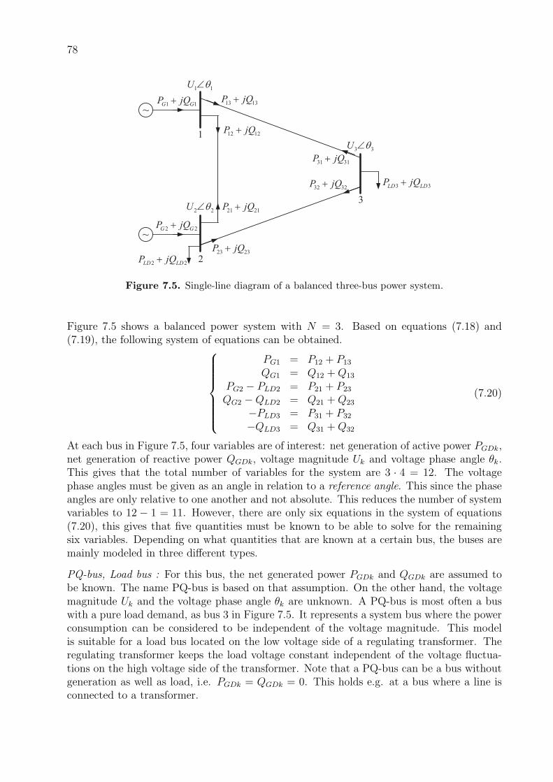
78
1 1G GP jQ+
1 1U qÐ
~
~2 2G GP jQ+
2 2LD LDP jQ+
3 3LD LDP jQ+
3 3U qÐ
2 2U qÐ
12 12P jQ+
21 21P jQ+
23 23P jQ+
32 32P jQ+
13 13P jQ+
31 31P jQ+
1
2
3
Figure 7.5. Single-line diagram of a balanced three-bus power system.
Figure 7.5 shows a balanced power system with N = 3. Based on equations (7.18) and(7.19), the following system of equations can be obtained.
PG1 = P12 + P13
QG1 = Q12 +Q13
PG2 − PLD2 = P21 + P23
QG2 −QLD2 = Q21 +Q23
−PLD3 = P31 + P32
−QLD3 = Q31 +Q32
(7.20)
At each bus in Figure 7.5, four variables are of interest: net generation of active power PGDk,net generation of reactive power QGDk, voltage magnitude Uk and voltage phase angle θk.This gives that the total number of variables for the system are 3 · 4 = 12. The voltagephase angles must be given as an angle in relation to a reference angle. This since the phaseangles are only relative to one another and not absolute. This reduces the number of systemvariables to 12 − 1 = 11. However, there are only six equations in the system of equations(7.20), this gives that five quantities must be known to be able to solve for the remainingsix variables. Depending on what quantities that are known at a certain bus, the buses aremainly modeled in three different types.
PQ-bus, Load bus : For this bus, the net generated power PGDk and QGDk are assumed tobe known. The name PQ-bus is based on that assumption. On the other hand, the voltagemagnitude Uk and the voltage phase angle θk are unknown. A PQ-bus is most often a buswith a pure load demand, as bus 3 in Figure 7.5. It represents a system bus where the powerconsumption can be considered to be independent of the voltage magnitude. This modelis suitable for a load bus located on the low voltage side of a regulating transformer. Theregulating transformer keeps the load voltage constant independent of the voltage fluctua-tions on the high voltage side of the transformer. Note that a PQ-bus can be a bus withoutgeneration as well as load, i.e. PGDk = QGDk = 0. This holds e.g. at a bus where a line isconnected to a transformer.

79
PU-bus, Generator bus : In a PU-bus, the net active power generation PGDk as well as thevoltage magnitude Uk are assumed to be known. This gives that the net reactive powergeneration QGDk and the voltage angle θk are unknown. In a PU-bus some sort of voltageregulating device must be connected since the voltage magnitude is independent of the netreactive power generation. For example, in a synchronous machine, the terminal voltage canbe regulated by changing the magnetizing current. In a system, voltage can be regulatedby using controllable components as controllable shunt capacitors and controllable shuntreactors. A standard component is called SVC, Static VAr Compensator. This componentchange the reactive power flow in order to regulate the bus voltage. Assume that bus2 in Figure 7.5 is modeled as a PU-bus. This gives that the active power generation ofthe generator as well as the active power consumption of the load are known. Also thereactive power consumption of the load is known. The bus voltage is constant due to themagnetization system of the generator. The generator may generate or consume reactivepower in such a way that the relation in equation (7.19) holds.
Uθ-bus, Slack bus : At a slack bus (only one bus in each system), the voltage magnitudeand the voltage phase angle are known and fixed. The voltage phase angle is chosen as a thereference phase angle in the system. Normally, the phase angle θk is set to zero. Unknownquantities are the net generation of both active and reactive power. At this bus, (as for thePU-bus) a voltage regulating component must be present. Since the active power is allowedto vary, a generator or an active power in-feed into the system is assumed to exist at this bus.Since this bus also is the only bus where the active power is allowed to vary, the slack buswill take care of the system losses since they are unknown. If the loads have been modeledin the load flow as constant power loads and a line is tripped, the only bus which will changethe active power generation is the slack bus. If bus 1 is chosen as slack bus in Figure 7.5,both PG1 and QG1 are unknown but the voltage U1 is given as well as the reference angleθ1 = 0.
Assume that M of the system N buses are PU-buses. A summary of the different bus typesis given in Table 7.1. As given in equations (7.3)–(7.4), the active and reactive power flow
Bus model Number Known quantities Unknown quantitiesUθ-bus, Slack bus 1 U , θ PGD, QGD
PU-bus, Generator bus M PGD, U QGD, θPQ-bus, Load bus N-M-1 PGD, QGD U , θ
Table 7.1. Bus types for load flow calculations
through a line can be expressed as a function of the voltage magnitude and voltage phaseangle at both ends of the line. Assume that the power system in Figure 7.5 is modeled insuch a way that bus 1 is a slack bus, bus 2 is a PU-bus and bus 3 is a PQ-bus. By usingthis bus type modeling, the system of equations (7.20) can be written as
PGD1(unknown) = P12(U1, θ1, U2, θ2) + P13(U1, θ1, U3, θ3)QG1(unknown) = Q12(U1, θ1, U2, θ2) +Q13(U1, θ1, U3, θ3)
PGD2 = P21(U1, θ1, U2, θ2) + P23(U2, θ2, U3, θ3)QGD2(unknown) = Q21(U1, θ1, U2, θ2) +Q23(U2, θ2, U3, θ3)
PGD3 = P31(U1, θ1, U3, θ3) + P32(U2, θ2, U3, θ3)QGD3 = Q31(U1, θ1, U3, θ3) +Q32(U2, θ2, U3, θ3)
(7.21)

80
where also θ2, U3 and θ3 are unknown quantities whereas the others are known. As given inequation (7.21), unknown power quantities appear only on the left hand side for buses mod-eled as slack and PU-bus. These quantities can be easily calculated when voltage magnitudesand angles are known. These equations are not contributing to the system of equations sincethey only give one extra equation, and one extra variable which easily can be calculated. Thesystem of equations in (7.21) can therefore be simplified to a system of equations containingunknown U and θ as
PGD2 = P21(U1, θ1, U2, θ2) + P23(U2, θ2, U3, θ3)PGD3 = P31(U1, θ1, U3, θ3) + P32(U2, θ2, U3, θ3)QGD3 = Q31(U1, θ1, U3, θ3) +Q32(U2, θ2, U3, θ3)
(7.22)
The system of equations given by (7.22) is non-linear since the expressions for power flowthrough a line (equation (7.3)–(7.4)) include squared voltages as well as trigonometric expres-sions. This system of equations can e.g. be solved by using the Newton-Raphson method.
The system of equations given by (7.22) can be generalized to a system containing N buses,of which M have a voltage regulating device in operation. A summary of this system is givenin Table 7.2. As indicated in Table 7.2, the system of equations contains as many unknown
Bus model Number Balance equations Unknown quantitiesPGDk =
∑Pkj QGDk =
∑Qkj Uk θk
Slack bus 1 0 0 0 0PU-bus M M 0 0 MPQ-bus N-M-1 N-M-1 N-M-1 N-M-1 N-M-1Total N 2N-M-2 2N-M-2
Table 7.2. Summary of equations and unknown quantities at load flow calculations
quantities as the number of equations, and by that, the system is solvable.
7.3 Power flow calculations of a simple two-bus system
As shown in section 7.2, constant power loads give a non-linear system of equations, andpower flow calculations for large power system requires soft-ware tools such as MATLABwhich will be used in this course. To understand the concept of power flow calculations, inthis section a simple two-bus system is studied. Since for power flow calculations, a bus busmust be a slack bus, there are therefore two possible bus-type combinations, namely, slackbus + PU-bus and slack bus + PQ-bus which can be analytically handled.
Consider the two-bus power system shown in Figure 7.6. The data given in Example 7.1 isused for this system. Let bus 1 be a slack bus with U 1 = 225 6 0 kV. Let also PLD2 = 80MW.

81
21Z
21shjb − 21shjb −
21S1 2
2
2 2
LD
LD LD
S
P jQ
=
+
Figure 7.6. Single-line diagram of a balanced two-bus power system.
7.3.1 Slack bus + PU-bus
This combination is of interest when the voltage magnitude is known at both buses and thenet active power (i.e. PGD) is known at one of the buses. This implies that the only unknownquantity is the voltage phase angle at the PU-bus, i.e. the bus having a known net activepower PGD.
Example 7.4 Let bus 2 be a PU-bus with U2 = 213.08 kV. Calculate the voltage phase angleat bus 2 (the same as Example 6.4). Find also Q21 in MVAr.
Solution
From equation (7.3) we have
P21 =R21
Z221
U22 +
U2 U1
Z21sin
(
θ21 − arctan
(R21
X21
))
⇒
θ2 = θ1 + arctan
(R21
X21
)
+ arcsin
(Z21
U2 U1
(
P21 −R21
Z221
U22
))
where,
P21 = PGD2 = (0− PLD2)/Sbase = −0.8 pu, arctanR21
X21= arctan
0.0079
0.0790= 5.71
Thus,
θ2 = 0 + 5.71 + arcsin
(0.0794
0.9470 · 1.0
(
−0.8− 0.0079
0.079420.94702
))
= −3.5724
From equation (7.4), we have
Q21 =
[(
−bsh−21 +X21
Z221
)
U22 − U2 U1
Z21cos
(
θ21 − arctan
(R21
X21
))]
Sbase
=
[(
−0.0759 +0.0790
0.07942
)
0.94702 − 0.9470 1.0
0.0794cos(−3.5724 − 5.71)
]
100
= −59.9793 MVAr, from MATLAB

82
7.3.2 Slack bus + PQ-bus
This combination is of interest when the voltage magnitude is known only at one of the busesand the net active and reactive power generation are known at the other bus.
Example 7.5 Now let bus 2 be a PQ-bus, and QLD2 = −Q21 where Q21 has been obtainedin Example 7.4. Calculate the voltage magnitude and phase angle at bus 2.
Solution
Based on equations (7.3) and (7.4), by eliminating θ21, the voltage magnitude U2 can beanalytically found, and it is given by
U22 = − a4
2a3
+
(−)
√(
a42a3
)2
− 1
a3(a21 + a22) (7.23)
where
a1 = −R21 P21 −X21Q21
a2 = −X21 P21 +R21Q21
a3 = (1−X21 bsh−21)2 +R2
21 b2sh−21
a4 = 2 · a1(1−X21 bsh−21)− U21 + 2a2R21 bsh−21
The voltage U2 can now be calculated as
U2 =+
(−)
√
U22 (7.24)
In our case,
a1 = −0.0079(−0.8)− 0.0790(−0.5998) = 0.0537
a2 = −0.0790(−0.8) + 0.0079(−0.6)) = 0.0585
a3 = (1− 0.0790 · 0.0759)2 + 0.00792 · 0.07592 = 0.9880
a4 = 2 · 0.0537(1− 0.0790 · 0.0759)− 1.02 +
+ 2 · 0.0585 · 0.0079 · 0.0759 = −0.8931
⇒U22 = 0.4520 +
(−)0.4449 = 0.8968
⇒U2 = +
(−)
√0.8968 = 0.9470
⇒U2 (kV) = 0.9470 · Ubase = 213.08 kV
The voltage phase angle can now be calculated in the same way as performed in Example7.4, which results in the the same answer.

83
Example 7.6 Use the data given in Example 7.5 with PD2 = 80 MW and QD2 ≈ 60 MVAr.Use these load levels as a base case and calculate the voltage U2 when the active and reactiveload demand are varying between 0–100 MW and 0–100 MVAr, respectively.
Solution
By using equations (7.23) and (7.24), the voltage can be calculated. The result is shown inFigure 7.7. The base case, i.e. PD2 = 80 MW and QD2 = 60 MVAr, is marked by circles on
0 10 20 30 40 50 60 70 80 90 100200
205
210
215
220
225
QD2=60 MVAr, PD2=0-100 MW
PD2=80 MW, QD2=0-100 MVAr
MW or MVAr
U2 [
kV
]
Figure 7.7. The voltage U2 as a function of PD2 and QD2.
both curves. As shown in the figure, the voltage drops at bus 2 as the load demand increases.The voltage at bus 2 is much more sensitive to a change in reactive load demand comparedto a change in active demand. If a shunt capacitor generating 10 MVAr is connected atbus 2 when having a reactive load demand of 60 MVAr, the net demand of reactive powerwill decrease to 50 MVAr and the bus voltage will increase by two kV, from 213 kV to 215kV. As discussed earlier in subsection 7.1.1, a reduced reactive power load demand will alsoreduce the losses on the line.
Example 7.7 Use the base case in Example 7.6, i.e. PD2 = 80 MW and QD2 = 60 MVAr.Calculate the voltage U2 when the series compensation of the line is varied in the interval0–100 %.
Solution
A series compensation of 0–100 %means that 0–100 % of the line reactance is compensated byseries capacitors. 0 % means no series compensation at all and 100 % means that Xc = X21.The voltage can be calculated by using equations (7.23) and (7.24). The result is shown inFigure 7.8. As shown in Figure 7.8, the voltage at bus 2 increases as the degree of seriescompensation increases. If the degree of compensation is 40 %, the voltage at bus 2 isincreased by 4.5 kV (= 2 %) from 213.1 kV to 217.6 kV.
When having short lines or when only interested in approximate calculations, the shuntcapacitance of a line can be neglected. In these conditions, bsh−21 in equation (7.23) is

84
0 10 20 30 40 50 60 70 80 90 100210
215
220
225
% compensation
U2 [
kV
]
Figure 7.8. The voltage U2 as a function of degree of compensation.
neglected, and the equation will be rewritten as
U2 =
√√√√U2
1 − 2a12
+
(−)
√(U21 − 2a12
)2
− (a21 + a22) (7.25)
where
a1 = −R21 P21 −X21Q21
a2 = −X21 P21 +R21 Q21
Example 7.8 Use the data given in Example 7.5. Calculate the magnitude of the voltageby using the approximate expression given by equation (7.25).
Solution
Equation (7.25) gives that
a1 = −0.0790(−0.8) + 0.0079(−0.6) = 0.0537
a2 = 0.0079(−0.6)− 0.0790(−0.8) = 0.0585
⇒U2 = 0.9410
⇒U2(kV) = 0.9410 · Ubase = 211.72 kV
i.e. the voltage becomes 0.6 % too low compared to the more accurate result.
Another approximation often used, is to neglect a2 in equation (7.25). That equation canthen be rewritten as
U2 ≈U1
2+
√
U21
4+R21 P21 +X21 Q21 (7.26)

85
Example 7.9 Use the same line as in Example 7.5. Calculate the voltage by using theapproximate expression given by equation (7.26).
Solution
Equation (7.26) gives that
U2 = 0.9430
⇒U2(kV ) = 0.9439 · Ubase = 212.18 kV
i.e. the calculated voltage is 0.4 % too low. As indicated in this example, equation (7.26)gives a good approximation of the voltage drop on the line. In the equation, it is also clearlygiven that the active and reactive load demand have influence on the voltage drop. Thereason why the voltage drop is more sensitive to a change in reactive power compared to achange in active power, is that the line reactance dominates the line resistance.
7.4 Newton-Raphson method
7.4.1 Theory
The Newton-Raphson method may be applied to solve for x1, x2, · · · , xn of the followingnon-linear equations,
g1(x1, x2, · · · , xn) = f1(x1, x2, · · · , xn)− b1 = 0
g2(x1, x2, · · · , xn) = f2(x1, x2, · · · , xn)− b2 = 0
...
gn(x1, x2, · · · , xn) = fn(x1, x2, · · · , xn)− bn = 0
(7.27)
or in the vector formg(x) = f(x)− b = 0 (7.28)
where
x =
x1
x2...xn
, g(x) =
g1(x)g2(x)...
gn(x)
, f(x) =
f1(x)f2(x)...
fn(x)
, b =
b1b2...bn
x is an n× 1 vector which contains variables, b is an n× 1 vector which contains constants,and f(x) is an n× 1 vector-valued function.
Taylor’s series expansion of (7.28) is the basis for the Newton-Raphson method of solving(7.28) in an iterative manner. From an initial estimate (or guess) x(0), a sequence of graduallybetter estimates x(1), x(2), x(3), · · · will be made that hopefully will converge to the solutionx∗.

86
Let x∗ be the solution of (7.28), i.e. g(x∗) = 0, and x(i) be an estimate of x∗. Let also∆x(i) = x∗ − x(i). Equation (7.28) can now be written as
g(x∗) = g(x(i) +∆x(i)) = 0 (7.29)
Taylor’s series expansion of (7.29) gives
g(x(i) +∆x(i)) = g(x(i)) + JAC(x(i))∆x(i) = 0 (7.30)
where
JAC(x(i)) =
[∂g(x)
∂x
]
x=x(i)
=
∂g1(x)∂x1
· · · ∂g1(x)∂xn
.... . .
...∂gn(x)∂x1
· · · ∂gn(x)∂xn
x=x(i)
(7.31)
is called the jacobian of g.
From (7.30), ∆x(i) can be calculated as follows
JAC(x(i))∆x(i) = 0− g(x(i)) = ∆g(x(i)) ⇒ (7.32)
∆x(i) =[
JAC(x(i))]−1
∆g(x(i)) (7.33)
Since g(x(i)) = f(x(i))− b, ∆g(x(i)) is given by
∆g(x(i)) = b− f(x(i)) = −g(x(i)) (7.34)
Furthermore, since b is constant, JAC(x(i)) is given by
JAC(x(i)) =
[∂g(x)
∂x
]
x=x(i)
=
[∂f(x)
∂x
]
x=x(i)
=
∂f1(x)∂x1
· · · ∂f1(x)∂xn
.... . .
...∂fn(x)∂x1
· · · ∂fn(x)∂xn
x=x(i)
(7.35)
Therefore, ∆x(i) can be calculated as follows
∆x(i) =
∆x(i)1...
∆x(i)n
=
∂f1(x)∂x1
· · · ∂f1(x)∂xn
.... . .
...∂fn(x)∂x1
· · · ∂fn(x)∂xn
−1
x=x(i)
b1 − f1(x(i)1 , · · · , x(i)
n )...
bn − fn(x(i)1 , · · · , x(i)
n )
(7.36)
Finally, the following is obtained
i = i+ 1
x(i) = x(i−1) +∆x(i−1)
The intention is that x(1) will estimate the solution x∗ better than what x(0) does. In thesame manner, x(2), x(3) , · · · can be determined until a specified condition is satisfied. Thus,we obtain an iterative method according to the flowchart in Figure 7.9.

87
Yes
No
( )Give ix
Set 0i =
( )ix x=
Step 1
Step 2
Step Final
( )Calculate ( )ig x∆
( )Is the magnitude of the all entries of ( )
less than a small positve number ?
ig x∆
( ) ( 1) ( 1)
1
i i i
i i
x x x− −
= +
= + ∆
Step 3
Step 4( )Calculate ix∆
Step 5
( )Calculate iJAC
Figure 7.9. Flowchart for the Newton-Raphson method.
Example 7.10 Using the Newton-Raphson method, solve for x of the equation
g(x) = k1 x+ k2 cos(x− k3)− k4 = 0
Let k1 = −0.2, k2 = 1.2, k3 = −0.07, k4 = 0.4 and ǫ = 10−4.
Solution
This equation is of the form given by (7.28), with f(x) = k1 x+ k2 cos(x− k3) and b = k4.
Step 1
Set i = 0 and x(i) = x(0) = 0.0524 (radians), i.e. 3 (degrees).
Step 2
∆g(x(i)) = b− f(x(i)) = 0.4− [(−0.2 ∗ 0.0524) + 1.2 cos(0.0524 + 0.07)] = −0.7806
Go to Step 3 since |∆g(x(i))| > ǫ
Step 3
JAC(x(i)) =[∂f∂x
]
x=x(i) = −0.2− 1.2 sin(0.0524 + 0.07) = −0.3465
Step 4
∆x(i) =[
JAC(x(i))]−1
∆g(x(i)) = −0.7806−0.3465
= 2.2529
Step 5
i = i+ 1 = 0 + 1 = 1x(i) = x(i−1) +∆x(i−1) = 0.0524 + 2.2529 = 2.3053. Go to Step 2

88
After 5 iterations, i.e. i = 5, it was found that |∆g(x(i))| < ǫ for x(5) = 0.9809 (rad.).Therefore, the solution becomes x = 0.9809 (rad.) or x = 56.2000 (deg.).
MATLAB-codes for this example can be found in Appendix A.
Comments on Example 7.10
Figure 7.10 shows variations of g(x) versus x. The figure shows that the system (or equation)has only three solutions, i.e. the points at which g(x) = 0. Due to practical issues, x∗ indictedwith (O) in the figure is the interesting solution.
−400 −300 −200 −100 0 100 200 300 400−2.5
−2
−1.5
−1
−0.5
0
0.5
1
1.5
2
2.5
x
g(x)
x*
Figure 7.10. Variations of g(x) vs. x.
Figure 7.11 shows how the equation is solved by the Newton-Raphson method.
We first guess the initial estimate x(0). In this case x(0) = 0.0524 (rad.), i.e 3 (deg.). The
tangent to g(x) through the point(x(0) , g(x(0))
), i.e. g′(x(0)) =
[dg(x)dx
]
x=x(0)= JAC(x(0)),
intersects the x–axis at point x(1). The equation for this tangent is given by
Y − g(x(0)) = g′(x(0)) ∗ (x− x(0))
The intersection point x(1) is obtained by setting Y = 0, i.e.
x(1) = x(0) − g(x(0))
g′(x(0))= x(0) −
(g′(x(0))
)−1g(x(0))
∆x(0) = x(1) − x(0) = −(g′(x(0))
)−1g(x(0)) =
[
JAC(x(0))]−1
∆g(x(0))
In a similar manner, x(2) can be obtained which is hopefully a better estimate than x(1). Asshown in the figure, from x(2) we obtain x(3) which is a better estimate of x∗ than what x(2)
does. This iterative method will be continued until |∆g(x)| < ǫ.
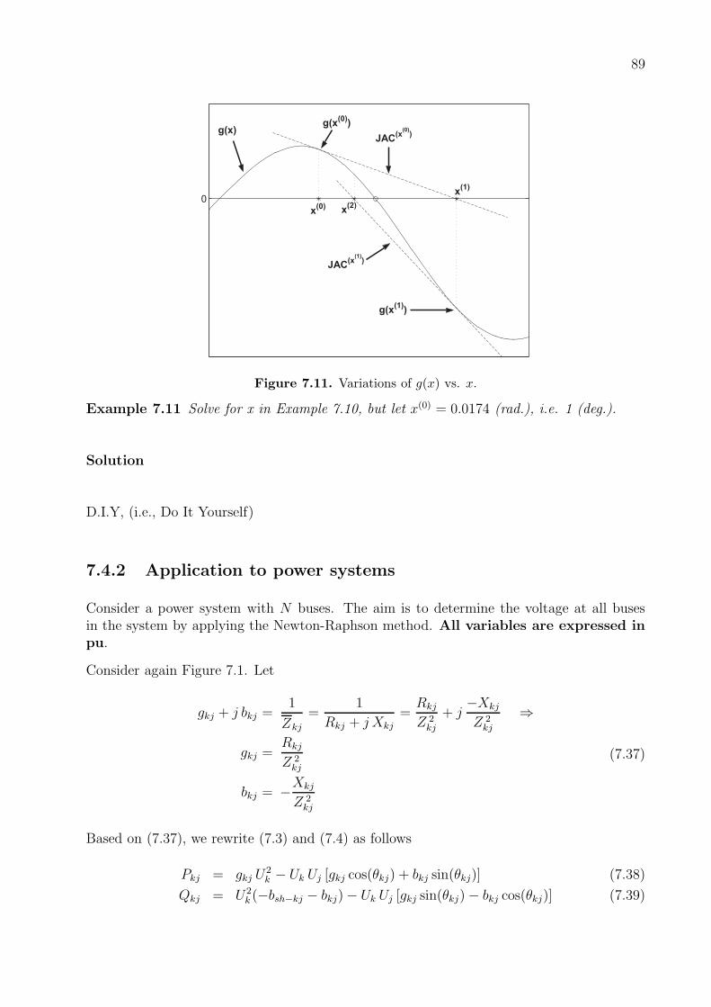
89
0
g(x)
x(0)
x(1)
x(2)
g(x(0))
JAC(x(0))
g(x(1))
JAC(x(1))
Figure 7.11. Variations of g(x) vs. x.
Example 7.11 Solve for x in Example 7.10, but let x(0) = 0.0174 (rad.), i.e. 1 (deg.).
Solution
D.I.Y, (i.e., Do It Yourself)
7.4.2 Application to power systems
Consider a power system with N buses. The aim is to determine the voltage at all busesin the system by applying the Newton-Raphson method. All variables are expressed inpu.
Consider again Figure 7.1. Let
gkj + j bkj =1
Zkj
=1
Rkj + j Xkj=
Rkj
Z 2kj
+ j−Xkj
Z 2kj
⇒
gkj =Rkj
Z 2kj
bkj = −Xkj
Z 2kj
(7.37)
Based on (7.37), we rewrite (7.3) and (7.4) as follows
Pkj = gkj U2k − Uk Uj [gkj cos(θkj) + bkj sin(θkj)] (7.38)
Qkj = U2k (−bsh−kj − bkj)− Uk Uj [gkj sin(θkj)− bkj cos(θkj)] (7.39)

90
The current through the line, and the losses in the line can be calculated by
Ikj =Pkj − j Qkj
U∗k
(7.40)
Plkj = Pkj + Pjk (7.41)
Qlkj = Qkj +Qjk (7.42)
Consider again Figure 7.4. Let Y = G+ jB denote the admittance matrix of the system (orY-matrix), where Y is an N ×N matrix, i.e. the system has N buses. The relation betweenthe injected currents into the buses and the voltages at the buses is given by I = Y U , seesection 4.1. Therefore, the injected current into bus k is given by Ik =
∑Nj=1 Y kj U j.
The injected complex power into bus k can now be calculated by
Sk = Uk I∗k = Uk
N∑
j=1
Y∗kjU
∗j = Uk
N∑
j=1
(Gkj − jBkj)Uj(cos(θkj) + j sin(θkj))
=
(
Uk
N∑
j=1
Uj [Gkj cos(θkj) +Bkj sin(θkj)]
)
+ j
(
Uk
N∑
j=1
Uj [Gkj sin(θkj)− Bkj cos(θkj)]
)
Let Pk denote the real part of Sk, i.e. the injected active power, and Qk denote the imaginarypart of Sk, i.e. the injected reactive power, as follows:
Pk = Uk
N∑
j=1
Uj [Gkj cos(θkj) +Bkj sin(θkj)]
Qk = Uk
N∑
j=1
Uj [Gkj sin(θkj)− Bkj cos(θkj)]
(7.43)
Note that Gkj = −gkj and Bkj = −bkj for k 6= j. Furthermore,
Pk =N∑
j=1
Pkj
Qk =N∑
j=1
Qkj
Equations (7.18) and (7.19) can now be rewritten as
Pk − PGDk = 0
Qk −QGDk = 0(7.44)

91
which are of the form given in equation (7.28), where
x =
θ
U
=
θ1...θN
U1...
UN
, f(θ, U) =
fP (θ, U)
fQ(θ, U)
=
P1...
PN
Q1...
QN
, b =
bP
bQ
=
PGD1...
PGDN
QGD1...
QGDN
(7.45)
the aim is to determine x = [θ U ]T by applying the Newton-Raphson method.
Assume that there are 1 slack bus and M PU-buses in the system. Therefore, θ becomes an(N − 1)× 1 vector and U becomes an (N − 1−M)× 1 vector, why?
Based on (7.34), we define the following:
∆Pk = PGDk − Pk k 6= slack bus
∆Qk = QGDk −Qk k 6= slack bus and PU-bus(7.46)
Based on (7.35), the jacobian matrix is given by
JAC =
∂fP (θ,U)∂θ
∂fP (θ,U)∂U
∂fQ(θ,U)
∂θ
∂fQ(θ,U)
∂U
=
H N ′
J L′
(7.47)
where,H is an (N − 1)× (N − 1) matrixN ′ is an (N − 1)× (N −M − 1) matrixJ is an (N −M − 1)× (N − 1) matrixL′ is an (N −M − 1)× (N −M − 1) matrix
The entries of these matrices are given by:
Hkj =∂Pk
∂θjk 6= slack bus j 6= slack bus
N ′kj =
∂Pk
∂Ujk 6= slack bus j 6= slack bus and PU-bus
Jkj =∂Qk
∂θjk 6= slack bus and PU-bus j 6= slack bus
L′kj =
∂Qk
∂Ujk 6= slack bus and PU-bus j 6= slack bus and PU-bus
Based on (7.32), (7.46) and (7.47), the following is obtained[H N ′
J L′
][∆θ∆U
]
=
[∆P∆Q
]
(7.48)
To simplify the entries of the matrices N ′ and L′, these matrices are multiplied with U .Then, (7.48) can be rewritten as
[H NJ L
][∆θ∆UU
]
=
[H NJ L
][∆θ∆U ′
]
=
[∆P∆Q
]
(7.49)

92
where,for k 6= j
Hkj =∂Pk
∂θj= Uk Uj [Gkj sin(θkj)− Bkj cos(θkj)]
Nkj = Uj N′kj = Uj
∂Pk
∂Uj= Uk Uj [Gkj cos(θkj) +Bkj sin(θkj)]
Jkj =∂Qk
∂θj= −Uk Uj [Gkj cos(θkj) +Bkj sin(θkj)]
Lkj = Uj L′kj = Uj
∂Qk
∂Uj= Uk Uj [Gkj sin(θkj)− Bkj cos(θkj)]
(7.50)
and for k = jHkk =
∂Pk
∂θk= −Qk − BkkU
2k
Nkk = Uk∂Pk
∂Uk= Pk +GkkU
2k
Jkk =∂Qk
∂θk= Pk −GkkU
2k
Lkj = Uk∂Qk
∂Uk= Qk − BkkU
2k
(7.51)
Now based on (7.36), the following is obtained:
[∆θ∆UU
]
=
[∆θ∆U ′
]
=
[H NJ L
]−1[∆P∆Q
]
(7.52)
Finally, U and θ will be updated as follows:
θk = θk +∆θk k 6= slack busUk = Uk (1 + ∆U ′
k) k 6= slack bus and PU-bus(7.53)
7.4.3 Newton-Raphson method for solving power flow equations
Newton-Raphson method can be applied to non-linear power flow equations as follows:
• Step 1
1a) Read bus and line data. Identify slack bus (i.e. Uθ-bus), PU-buses and PQ-buses.
1b) Build the Y-matrix and calculate the net productions, i.e. PGD = PG − PLD andQGD = QG −QLD.
1c) Give the initial estimate of the unknown variables, i.e. U for PQ-buses and θ forPU- and PQ-buses. It is very common to set U = Uslack and θ = θslack. However,the flat initial estimate may also be applied, i.e. U = 1 and θ = 0.
1d) Go to Step 2.
• Step 2

93
2a) Calculate the injected power into each bus by equation (7.43).
2b) Calculate the difference between the net production and the injected power foreach bus, i.e. ∆P and ∆Q by equation (7.46).
2c) Is the magnitude of all entries of [∆P ∆Q]T less than a specified small positiveconstant ǫ ?
∗ If yes, go to Step Final.
∗ if no, go to Step 3.
• Step 3
3a) Calculate the jacobian by equations (7.50) and (7.51).
3b) Go to Step 4.
• Step 4
4a) Calculate [∆θ ∆U ′]T by equation (7.52).
4b) Go to Step 5.
• Step 5
5a) Update U and θ by equation (7.53).
5b) Go till Step 2.
• Step Final
– Calculate the generated powers, i.e. PG (MW) and QG (MVAr) in the slack bus,and QG (MVAr) in the PU-buses by using equation (7.44).
– Calculate the power flows (MW, MVAr) by using equations (7.38) and (7.39).
– Calculate active power losses (MW) by using equation (7.41).
– Give all the voltage magnitudes (kV) and the voltage phase angles (degrees).
– Print out the results.
Example 7.12 Consider the power system shown in Figure 7.12. Let Sbase = 100 MVA,and Ubase = 220 kV.
1 2
~ ~
Figure 7.12. Single-line diagram of a balanced two-bus power system.
The following data (all in pu) is known:
• Line between Bus 1 and Bus 2: short line, Z12 = 0.02 + j 0.2

94
• Bus 1: slack bus, U1 = 1, θ1 = 0, PLD1 = 0.2, QLD1 = 0.02
• Bus 2: PU-bus, U2 = 1, PG2 = 1, PLD2 = 2, QLD2 = 0.2
By applying Newton-Raphson method, calculate θ2, PG1, QG1, QG2 and the active powerlosses in the system after 3 iterations.
Solution
MATLAB-codes for this example can be found in Appendix A.
Step 11a) bus 1 is a slack bus , bus 2 is a PU-bus , U1 = 1, U2 = 1, θ1 = 0.
1b)
Y =
1Z12
− 1Z12
− 1Z12
1Z12
=
G11 + j B11 G12 + j B12
G21 + j B21 G22 + j B22
=
=
0.4950− j 4.9505 −0.4950 + j 4.9505
−0.4950 + j 4.9505 0.4950− j 4.9505
= G+ jB
PGD2 = PG2 − PLD2 = 1− 2 = −1
No QGD since there is no PQ-bus in the system.
1c)Since the system has only one slack bus and one PU-bus, the phase angle of the PU-bus isthe only unknown variable. As an initial value , let θ2 = 0.
Iteration 1
Step 22a)
P2 = U2 U1 [G21 cos(θ2 − θ1) +B21 sin(θ2 − θ1)] + U22 G22 =
= 1 ∗ 1 ∗ [−0.4950 ∗ cos(0− 0) + 4.9505 ∗ sin(0− 0)] + 12 ∗ 0.4950 = 0
2b)∆P = ∆P2 = PGD2 − P2 = −1− 0 = −1
Step 3
Q2 = U2 U1 [G21 sin(θ2 − θ1)− B21 cos(θ2 − θ1)]− U22 B22 =
= 1 ∗ 1 ∗ [−0.4950 ∗ sin(0− 0)− 4.9505 ∗ cos(0− 0)]− 12 ∗ (−4.9505) = 0
H =∂P2
∂θ2= −Q2 −B22U
22 = −0− (−4.9505 ∗ 12) = 4.9505
JAC =[H]=[4.9505
]

95
Step 4
∆θ2 = H−1∆P2 =−1
4.9505= −0.2020
Step 5θ2 = θ2 +∆θ2 = 0− 0.2020 = −0.2020
Iteration 2Step 22a)
P2 = U2 U1 [G21 cos(θ2 − θ1) +B21 sin(θ2 − θ1)] + U22 G22 =
= 1 ∗ 1 ∗ [−0.4950 ∗ cos(−0.2020− 0) + 4.9505 ∗ sin(−0.2020− 0)] + 12 ∗ 0.4950 = −0.9831
2b)∆P = ∆P2 = PGD2 − P2 = −1− (−0.9831) = −0.0169
Step 3
Q2 = U2 U1 [G21 sin(θ2 − θ1)− B21 cos(θ2 − θ1)]− U22 B22 =
= 1 ∗ 1 ∗ [−0.4950 ∗ sin(−0.2020− 0)− 4.9505 ∗ cos(−0.2020− 0)]− 12 ∗ (−4.9505) = 0.2000
H =∂P2
∂θ2= −Q2 −B22U
22 = −0.2000− (−4.9505 ∗ 12) = 4.7505
JAC =[H]=[4.7505
]
Step 4
∆θ2 = H−1∆P2 =−0.0169
4.7505= −0.0035
Step 5θ2 = θ2 +∆θ2 = −0.2020− 0.0035 = −0.2055
Iteration 3Step 22a)
P2 = U2 U1 [G21 cos(θ2 − θ1) +B21 sin(θ2 − θ1)] + U22 G22 =
= 1 ∗ 1 ∗ [−0.4950 ∗ cos(−0.2055− 0) + 4.9505 ∗ sin(−0.2055− 0)] + 12 ∗ 0.4950 = −1.0000
2b)
∆P = ∆P2 = PGD2 − P2 = −1 − (−1.0000) ≈ 0 (in MATLAB ∆P2 = −9.3368 ∗ 10−6)
Step 3
Q2 = U2 U1 [G21 sin(θ2 − θ1)− B21 cos(θ2 − θ1)]− U22 B22 =
= 1 ∗ 1 ∗ [−0.4950 ∗ sin(−0.2055− 0)− 4.9505 ∗ cos(−0.2055− 0)]− 12 ∗ (−4.9505) = 0.2053
H =∂P2
∂θ2= −Q2 −B22U
22 = −0.2053− (−4.9505 ∗ 12) = 4.7452
JAC =[H]=[4.7452
]

96
Step 4
∆θ2 = H−1∆P2 =−9.3368 ∗ 10−6
4.7452= −1.9676 ∗ 10−6 ≈ 0
Step 5θ2 = θ2 + 0 = −0.2055− 0 = −0.2055
Now go to Step Final
Step Final
P1 = U1 U2 [G12 cos(θ1 − θ2) +B12 sin(θ1 − θ2)] + U21 G11 =
= 1 ∗ 1 ∗ [−0.4950 ∗ cos(0 + 0.2055) + 4.9505 ∗ sin(0 + 0.2055)] + 12 ∗ 0.4950 = 1.0208
Q1 = U1 U2 [G12 sin(θ1 − θ2)− B12 cos(θ1 − θ2)]− U21 B11 =
= 1 ∗ 1 ∗ [−0.4950 ∗ sin(0 + 0.2055)− 4.9505 ∗ cos(0 + 0.2055)]− 12 ∗ (−4.9505) = 0.0032
Q2 = U2 U1 [G21 sin(θ2 − θ1)− B21 cos(θ2 − θ1)]− U22 B22 =
= 1 ∗ 1 ∗ [−0.4950 ∗ sin(−0.2055− 0)− 4.9505 ∗ cos(−0.2055− 0)]− 12 ∗ (−4.9505) = 0.2053
PG1 = (P1 + PLD1) ∗ Sbase = (1.0208 + 0.2) ∗ 100 = 122.08 MW (in MATLAB PG1=122.0843)
QG1 = (Q1 +QLD1) ∗ Sbase = (0.0032 + 0.02) ∗ 100 = 2.32 MVAr (in MATLAB QG1=2.3171)
QG2 = (Q2 +QLD2) ∗ Sbase = (0.2053 + 0.2) ∗ 100 = 40.53 MVAr (in MATLAB QG2=40.5255)
g = −G , b = −B and bsh−12 = 0
P12 =(g12 U
21 − U1 U2 [g12 cos(θ1 − θ2) + b12 sin(θ1 − θ2)]
)∗ Sbase =
=(0.4950 ∗ 12 − 1 ∗ 1 ∗ [0.4950 ∗ cos(0 + 0.2055)− 4.9505 ∗ sin(0 + 0.2055)]
)∗ 100 =
= 102.0843 MW
P21 =(g21 U
22 − U2 U1 [g21 cos(θ2 − θ1) + b21 sin(θ2 − θ1)]
)∗ Sbase =
=(0.4950 ∗ 12 − 1 ∗ 1 ∗ [0.4950 ∗ cos(−0.2055− 0)− 4.9505 ∗ sin(−0.2055− 0)]
)∗ 100 =
= −100 MW
Q12 =((−bsh−12 − b12)U
21 − U1 U2 [g12 sin(θ1 − θ2)− b12 cos(θ1 − θ2)]
)∗ Sbase =
=((−0 + 4.9505) ∗ 12 − 1 ∗ 1 ∗ [0.4950 ∗ sin(0 + 0.2055) + 4.9505 ∗ cos(0 + 0.2055)]
)∗ 100 =
= 0.3171 MVAr
Q21 =((−bsh−12 − b21)U
22 − U2 U1 [g21 sin(θ2 − θ1)− b21 cos(θ2 − θ1)]
)∗ Sbase =
=((−0 + 4.9505) ∗ 12 − 1 ∗ 1 ∗ [0.4950 ∗ sin(−0.2055− 0) + 4.9505 ∗ cos(−0.2055− 0)]
)∗ 100
= 20.5255 MVAr
P totLoss = P12 + P21 = 102.0843− 100 = 2.0843 MW
or
P totLoss = (PG1 + PG2)− (PLD1 + PLD2) = (122.0843 + 100)− (20 + 200) = 2.0843 MW
ANG = [θ1 θ2] ∗180
π= [0 − 0.2055] ∗ 180
π= [0 − 11.7771]
VOLT = [U1 U2] ∗ Ubase = [1 1] ∗ 220 = [220 220]

97
Example 7.13 Consider again the power system shown in Figure 7.12. In this example, letbus 2 be a PQ-bus with the following data:
• Bus 2: PQ-bus, PG2 = 1, QG2 = 0.405255, PLD2 = 2, QLD2 = 0.2
Let also ε = 10−6. By applying Newton-Raphson method, calculate θ2, PG1, QG1, QG2 andthe active power losses.
Solution
See the MATLAB-codes in Appendix A.
Step 11a) bus 1 is a slack bus , bus 2 is a PQ-bus , U1 = 1 and θ1 = 0.
1b)
Y =
G11 + j B11 G12 + j B12
G21 + j B21 G22 + j B22
= G+ jB
PGD2 = PG2 − PLD2
QGD2 = QG2 −QLD2
1c)Since the system has only one PQ-bus, the voltage and phase angle of bus 2 are the unknownvariables. As an initial value , let θ2 = 0 and U2 = 1.
Step 22a)
P2 = U2 U1 [G21 cos(θ2 − θ1) +B21 sin(θ2 − θ1)] + U22 G22
Q2 = U2 U1 [G21 sin(θ2 − θ1)− B21 cos(θ2 − θ1)]− U22 B22
2b)
∆P = ∆P2 = PGD2 − P2
∆Q = ∆Q2 = QGD2 −Q2
Step 3As long as |∆P2| > ε and |∆Q2| > ε, perform Step 3 as follows:
H = −Q2 −B22U22
N = P2 +G22U22
J = P2 −G22U22
L = Q2 − B22U22
JAC =
[H NJ L
]
[∆θ2∆U ′
2
]
= JAC−1
[∆P2
∆Q2
]

98
Next, update ∆P2 and ∆Q2 based on updated θ2 and U2 (i.e Steps 4-5) as follows:
θ2 = θ2 +∆θ2
U2 = U2 (1 + ∆U ′2)
P2 = U2 U1 [G21 cos(θ2 − θ1) +B21 sin(θ2 − θ1)] + U22 G22
Q2 = U2 U1 [G21 sin(θ2 − θ1)− B21 cos(θ2 − θ1)]− U22 B22
∆P = ∆P2 = PGD2 − P2
∆Q = ∆Q2 = QGD2 −Q2
and check if |∆P2| < ε and |∆Q2| < ε.
Step Final
See Step Final in Example 7.12.
In the next examples, it will be shown that how the ”fsolve” function in MATLAB can beused for solving non-linear power flow equations.
Example 7.14 Consider the power system shown in Figure 7.13. Let the base power beSbase = 100 MVA, the base voltage be Ubase = 220 kV. Let also, bus 1 be a slack bus.
1
2
3
~
4
System 1 System 2
Figure 7.13. Single-line diagram of a balanced four-bus power system.
The system data (in MW, MVAr, kV, Ω and S) is given as follows:
• Line between Bus 1 and Bus 2: Z12 = 5 + j 65 , bsh−12 = 0.0002
• Line between Bus 1 and Bus 3: Z13 = 4 + j 60 , bsh−13 = 0.0002
• Line between Bus 2 and Bus 3: Z23 = 5 + j 68 , bsh−23 = 0.0002
• Line between Bus 3 and Bus 4: Z34 = 3 + j 30, short line
• Bus 1: U1 = 220, θ1 = 0, PLD1 = 10, QLD1 = 2
• Bus 2: PLD2 = 90, QLD2 = 10
• Bus 3: PLD3 = 80, QLD3 = 10
• Bus 4: PLD4 = 50, QLD4 = 10

99
Use ”fsolve” function in MATLAB, and find
a) the unknown voltage magnitudes and voltage phase angles,
b) the generated active and reactive powers at the slack bus, and the generated reactivepowers at PU-buses (if any),
c) the total active power losses, and the losses in System1 and System 2,
d) the changes (in % compared to the obtained results in task c)) of power losses in bothsystems, for an active load increased at bus 2 with 30 MW, i.e. P new
LD2 = 120 MW.
e) Let PLD2 = 90 MW. Re-do task d) for a reactive load increased at bus 3 with 10 MVAr,i.e. Qnew
LD3 = 20 MVAr.
Solution
MATLAB-codes for this example can be found in Appendix A.
For using ”fsolve”, you may need two MATLAB-files, one main file and one for solving x in0 = g(x) by ”fsolve” function, (see the MATLAB-codes in Appendix A). In the second fileyou need to define x and g(x) as follows:
x = [θ2 θ3 θ4 U2 U3 U4]
0 = g1(x) = P2 − PGD2 , (active power mismatch at bus 2, see equation (7.44))
0 = g2(x) = P3 − PGD3 , (active power mismatch at bus 3)
0 = g3(x) = P4 − PGD4 , (active power mismatch at bus 4)
0 = g4(x) = Q2 −QGD2 , (reactive power mismatch at bus 2)
0 = g5(x) = Q3 −QGD3 , (reactive power mismatch at bus 3)
0 = g6(x) = Q4 −QGD4 , (reactive power mismatch at bus 4)
where, Pk and Qk can be obtained based on equation (7.43).
a) U1 = 1.0000× Ubase = 220.0000 kV, θ1 = 0,U2 = 0.9864× Ubase = 216.9990 kV, θ2 = −7.8846,U3 = 0.9794× Ubase = 215.4704 kV, θ3 = −8.7252,U4 = 0.9693× Ubase = 213.2499 kV, θ4 = −10.5585,
b) Slack bus (bus 1): PG1 = 232.4938 MW, QG1 = 9.6185 MVAr
c) P Sys1Loss = 0.1715 MW , P Sys2
Loss = 2.3222 MW , P totLoss = 2.4938 MW
d) P Sys1Loss = 0.1729 MW ⇒ ∆P Sys1
Loss = 0.8163%
P Sys2Loss = 3.0236 MW ⇒ ∆P Sys2
Loss = 30.2041%
P totLoss = 3.1966 MW ⇒ ∆P tot
Loss = 28.1830%

100
e) P Sys1Loss = 0.1749 MW ⇒ ∆P Sys1
Loss = 1.9825%
P Sys2Loss = 2.3629 MW ⇒ ∆P Sys2
Loss = 1.7526%
P totLoss = 2.5378 MW ⇒ ∆P tot
Loss = 1.7685%
Example 7.15 Consider again the power system in Example 7.14. The System 1 operatoris interested in the results of the power flow calculations when installing a controllable shuntcapacitor at bus 3 to keep the voltage at its rated (or nominal) value, i.e. U3 = 220 kV.Re-do the tasks in Example 7.14, and also find the size of the shunt capacitor Bsh in S.
Solution
In this example, bus 3 will be considered as a PU-bus with U3 = 220 kV. MATLAB-codes forthis example can be found in Appendix A. Note that only the changes of the MATLAB-codescompared to the MATLAB-codes for Example 7.14 are given.
a) U1 = 1.0000× Ubase = 220.0000 kV, θ1 = 0,U2 = 0.9968× Ubase = 219.2882 kV, θ2 = −7.8192,U3 = 1.0000× Ubase = 220.0000 kV, θ3 = −8.6473,U4 = 0.9901× Ubase = 217.8306 kV, θ4 = −10.4051,
b) Slack bus (bus 1): PG1 = 232.4490 MW, QG1 = −14.7469 MVArPU-buses (bus 3): QG3 = 22.5772 MVAr and Bsh = 0.00046647 S
c) P Sys1Loss = 0.1644 MW , P Sys2
Loss = 2.2846 MW , P totLoss = 2.4490 MW
d) P Sys1Loss = 0.1644 MW ⇒ ∆P Sys1
Loss = 0%
P Sys2Loss = 2.9622 MW ⇒ ∆P Sys2
Loss = 29.6595%
P totLoss = 3.1266 MW ⇒ ∆P tot
Loss = 27.6684%
e) P Sys1Loss = 0.1644 MW ⇒ ∆P Sys1
Loss = 0%
P Sys2Loss = 2.2846 MW ⇒ ∆P Sys2
Loss = 0%
P totLoss = 2.4490 MW ⇒ ∆P tot
Loss = 0%
Example 7.16 Consider the power system described in Example 7.15. Now, both systemoperators are interested in the results of the power flow calculations when the generator at bus1 has a fixed generation with PG1 and QG1 obtained in Example 7.15, and a new generatoris installed at bus 4 to be a slack bus with U4 and θ4 obtained in Example 7.15. Re-do thetasks in Example 7.15.
Solution
In this example, bus 1 will be considered as a PQ-bus. After modifying the MATLAB-codesfor Example 7.15, the load flow simulations give the following results:

101
a) U1 = 1.0000× Ubase = 220.0000 kV, θ1 = 0,U2 = 0.9968× Ubase = 219.2882 kV, θ2 = −7.8192,U3 = 1.0000× Ubase = 220.0000 kV, θ3 = −8.6473,U4 = 0.9901× Ubase = 217.8306 kV, θ4 = −10.4051,
b) Slack bus (bus 4): PG4 = 0 MW, QG4 = 0 MVArPU-buses (bus 3): QG3 = 22.5772 MVAr and Bsh = 0.00046647 S
c) P Sys1Loss = 0.1644 MW , P Sys2
Loss = 2.2846 MW , P totLoss = 2.4490 MW
d) P Sys1Loss = 0.0373 MW ⇒ ∆P Sys1
Loss = −77.3114%
P Sys2Loss = 2.3232 MW ⇒ ∆P Sys2
Loss = 1.6896%
P totLoss = 2.3605 MW ⇒ ∆P tot
Loss = −3.6137%
e) P Sys1Loss = 0.1644 MW ⇒ ∆P Sys1
Loss = 0%
P Sys2Loss = 2.2846 MW ⇒ ∆P Sys2
Loss = 0%
P totLoss = 2.4490 MW ⇒ ∆P tot
Loss = 0%
Some questions regarding the obtained results:
q1: Why is ∆P Sys1Loss = 0 in Example 7.15, task d), but not in Example 7.14 and Example
7.16?
q2: Why is ∆P totLoss = 0 in Example 7.15 and Example 7.16 , task e), but not in Example
7.14?
q3: Why have ∆P Sys1Loss and ∆P tot
Loss in Example 7.16, task d), decreased?
q4: In Example 7.15, does Bsh in tasks d) and e) have the same value as that obtained intask b)? Motivate your answer.
q5: Why are the obtained voltages in Example 7.15 and Example 7.16 identical?

102

Chapter 8
Symmetrical components
8.1 Definitions
Assume an arbitrary un-symmetric combination of three phases, exemplified by the currentsIa, Ib and Ic, as shown in Figure 8.1 a).
b)
1aI
1cI
1bI
aI
bI
cI
a)
2aI
c) d)
2cI
2bI
0aI
0bI
0cI
1aI 2aI0aI
1bI2bI
0bI
1cI
0cI2cI
Figure 8.1. Unbalanced current phasors expressed as the sum of positive-, negative-,and zero-sequence components.
Based on C. L. Fortesque’s theorem, a set of three unbalanced phasors in a three-phasesystem can be resolved into the following three balanced systems of phasors (or symmetricalcomponents) :
A. Positive-sequence components consisting of a balanced system of three phasors withthe same amplitude, and having a phase displacement of 120 and 240, respectively.The phase sequence is abca, as shown in Figure 8.1 b).
B. Negative-sequence components consisting of a balanced system of three phasors withthe same amplitude, and having a phase displacement of 240 and 120, respectively.The phase sequence is acba, as shown in Figure 8.1 c).
C. Zero-sequence components consisting of a balanced system of three phasors with thesame amplitude and phase, as shown in Figure 8.1 d).
The three balanced systems can be symbolized with 1 (positive-sequence), 2 (negative-sequence) and 0 (zero-sequence).
103

104
The result shown in Figure 8.1 can be mathematically expressed as :
Ia = Ia1 + Ia2 + Ia0
Ib = Ib1 + Ib2 + Ib0 (8.1)
Ic = Ic1 + Ic2 + Ic0
The three positive-sequence components can be denoted as
Ib1 = Ia1e−j120 (8.2)
Ic1 = Ia1ej120
The corresponding expressions for the negative- and zero-sequence components are as
Ib2 = Ia2ej120
Ic2 = Ia2e−j120 (8.3)
Ia0 = Ib0 = Ic0
By inserting equation (8.2) and (8.3) into equation (8.1), the following is obtained
Ia = Ia1 + Ia2 + Ia0
Ib = α2Ia1 + αIa2 + Ia0 (8.4)
Ic = αIa1 + α2Ia2 + Ia0
where,
α = ej120
= cos 120 + j sin 120 = −1
2+ j
√3
2(8.5)
The following expressions of the symbol α are valid
α2 = ej240
= e−j120 = −1
2− j
√3
2α3 = 1
1 + α + α2 = 0 (8.6)
α∗ = α2
(α2)∗ = α
Equation (8.4) can, by using matrix form, be written as
Iph= TIs (8.7)
where the matrix
T =
1 1 1α2 α 1α α2 1
(8.8)
is called the transformation matrix for the symmetrical components, (see also Appendix Bwhere various linear transformations are presented). The current vector
Iph=
IaIbIc
(8.9)

105
represents the current phasor of each phase whereas
Is =
Ia1Ia2Ia0
or just Is =
I−1
I−2
I−0
(8.10)
represents the symmetrical components of the phase a current from which (based on equa-tions (8.2)-(8.3)) the symmetrical components of the other phase currents can be obtained.
By using equation (8.7), the symmetrical components as a function of the phase currentscan be obtained by :
Is = T−1Iph(8.11)
where
T−1 =1
3
1 α α2
1 α2 α1 1 1
(8.12)
Of course, the symmetrical components can also be applied to voltages. Using the vectors
Uph=
Ua
U b
U c
and Us =
Ua1
Ua2
Ua0
or just Us =
U−1
U−2
U−0
(8.13)
for representing line-to-neutral voltage phasors and symmetrical components, respectively,the relation between them can be written as
Uph= TUs (8.14)
Us = T−1Uph(8.15)
Example 8.1 Calculate the symmetrical components for the following symmetrical voltages
Uph=
Ua
U b
U c
=
277 6 0
277 6 − 120
277 6 + 120
V (8.16)
Solution
By using equations (8.12) and (8.15), the symmetrical components of the voltage Uphcan
be calculated as
U−1
U−2
U−0
= Us = T−1Uph=
1
3
1 α α2
1 α2 α1 1 1
Ua
U b
U c
= (8.17)
=1
3
1 · 277 + 1 6 120 · 277 6 − 120 + 1 6 240 · 277 6 + 120
1 · 277 + 1 6 240 · 277 6 − 120 + 1 6 120 · 277 6 + 120
1 · 277 + 1 · 277 6 − 120 + 1 · 277 6 + 120
=
=
277 6 0
00

106
As given in the example, a symmetric three-phase system with a phase sequence of abc givesrise to a positive-sequence voltage only, having the same amplitude and angle as the voltagein phase a.
Example 8.2 For a Y0-connected three-phase load (Y0 means that the neutral point isgrounded either solidly or through an impedance), phase b is at one occasion disconnected.The load currents at that occasion are :
Iph=
IaIbIc
=
10 6 0
010 6 + 120
A (8.18)
Calculate the symmetrical components of the load current as well as the current through theneutral-ground conductor, In.
Solution
I−1
I−2
I−0
=1
3
1 · 10 6 0 + 1 6 120 · 0 + 1 6 240 · 10 6 + 120
1 · 10 6 0 + 1 6 240 · 0 + 1 6 120 · 10 6 + 120
1 · 10 6 0 + 1 · 0 + 1 · 10 6 + 120
= (8.19)
=
6.667 6 0
3.333 6 − 60
3.333 6 60
In = Ia + Ib + Ic = 10 6 0 + 0 + 10 6 + 120 = 10 6 60 = 3I−0 (8.20)
As given in the example, the current through the neutral-ground conductor is three timesas large as the zero-sequence current.
8.1.1 Power calculations under unbalanced conditions
Based on the voltage and current phasors of each phase, the three-phase complex power canbe calculated as
S = P + jQ = UaI∗a + U bI
∗b + U cI
∗c = Ut
phI∗ph
(8.21)
By introducing symmetrical components, the expression above can be converted to
S = UtphI∗ph
= (TUs)t(TIs)
∗ = UtsT
tT∗I∗s (8.22)
where t stands for transpose. The expression TtT∗ can be written as
TtT∗ =
1 α2 α1 α α2
1 1 1
1 1 1α α2 1α2 α 1
= 3
1 0 00 1 00 0 1
(8.23)
i.e. the transformation is not power invariant since UtphI∗ph
6= UtsI
∗s, see also Appendix B.
Equation (8.22) can be rewritten as
S = 3Uts I
∗s = 3U−1 I
∗−1 + 3U−2 I
∗−2 + 3U−0 I
∗−0 (8.24)

107
Since the magnitude of the line-to-line voltages are√3 times the line-to-neutral voltages and
Sbase =√3 · Ubase · Ibase, the introduction of the per-unit system gives that equation (8.24)
can be rewritten as
Spu =
√3(√3Us)
t · I∗s√3 · Ubase · Ibase
= Upu−1 I∗pu−1 + U pu−2 I
∗pu−2 + U pu−0 I
∗pu−0 pu (8.25)
This implies that the total power (in per-unit value) in an unbalanced system can be ex-pressed by the sum of the symmetrical components of power. The total power in physicalunit can be obtained by multiplying Spu with Sbase, i.e.
S = Spu Sbase = U pu−1 I∗pu−1 Sbase + Upu−2 I
∗pu−2 Sbase + U pu−0 I
∗pu−0 Sbase MVA (8.26)
8.2 Sequence circuits of power system components
8.2.1 Transformers
In the analysis of three-phase circuits under unbalanced conditions, the transformer is rep-resented by its positive-, negative- and zero-sequence impedances. These can be determinedby analyzing the three-phase transformer, e.g. the Y0-∆ connected shown in Figure 8.2.
aIa
b
c
n
A
C
B
bI
cI
eZ
eZ
eZ
nZ nI
Figure 8.2. Y0-∆ connected transformer with neutral point grounded through animpedance Zn.
The impedance Ze represents the equivalent impedance of each phase and consists of bothleakage reactance of the primary and secondary windings as well as the resistance of thewindings, i.e. the windings shown in the figure are considered as ideal windings. Themagnetizing current of the transformer can be neglected, i.e. the magnetizing impedance isassumed to be infinitely large.
By using the direction of currents as shown in Figure 8.2, the following expressions for thethree phases of the transformer can be held
∆Ua = IaZe + InZn
∆U b = IbZe + InZn (8.27)
∆U c = IcZe + InZn
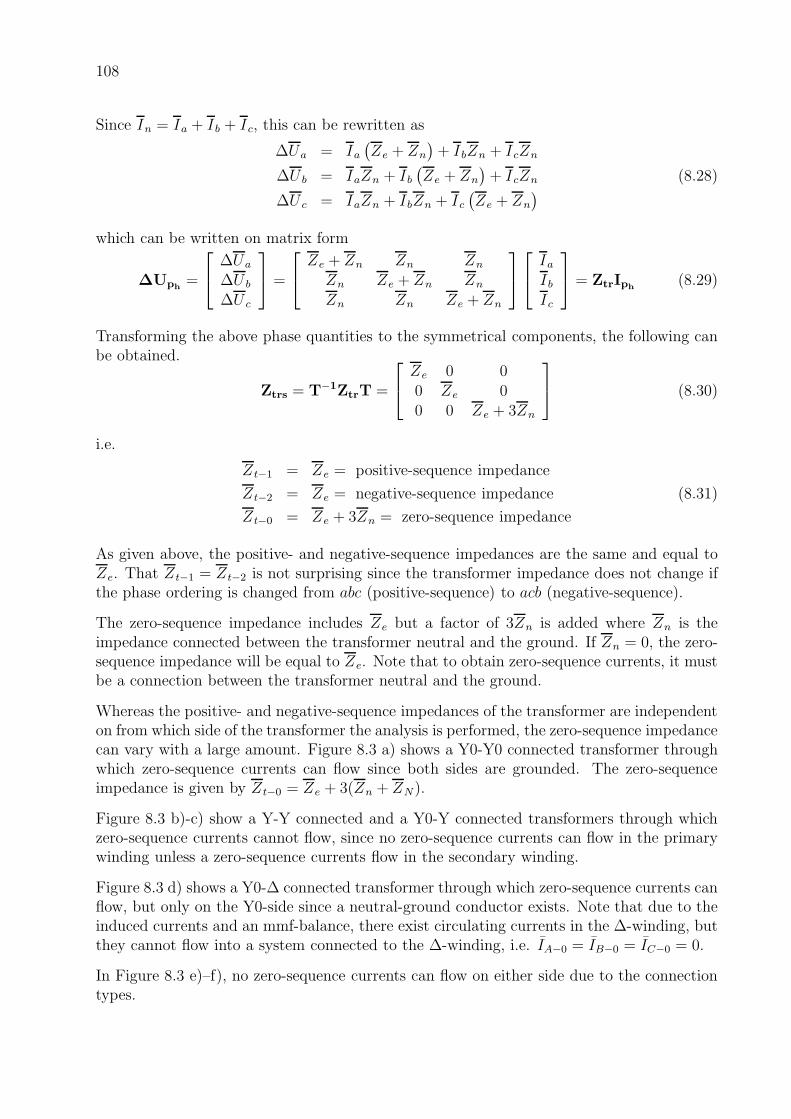
108
Since In = Ia + Ib + Ic, this can be rewritten as
∆Ua = Ia(Ze + Zn
)+ IbZn + IcZn
∆U b = IaZn + Ib(Ze + Zn
)+ IcZn (8.28)
∆U c = IaZn + IbZn + Ic(Ze + Zn
)
which can be written on matrix form
∆Uph=
∆Ua
∆U b
∆U c
=
Ze + Zn Zn Zn
Zn Ze + Zn Zn
Zn Zn Ze + Zn
IaIbIc
= ZtrIph(8.29)
Transforming the above phase quantities to the symmetrical components, the following canbe obtained.
Ztrs = T−1ZtrT =
Ze 0 00 Ze 00 0 Ze + 3Zn
(8.30)
i.e.
Zt−1 = Ze = positive-sequence impedance
Zt−2 = Ze = negative-sequence impedance (8.31)
Zt−0 = Ze + 3Zn = zero-sequence impedance
As given above, the positive- and negative-sequence impedances are the same and equal toZe. That Zt−1 = Zt−2 is not surprising since the transformer impedance does not change ifthe phase ordering is changed from abc (positive-sequence) to acb (negative-sequence).
The zero-sequence impedance includes Ze but a factor of 3Zn is added where Zn is theimpedance connected between the transformer neutral and the ground. If Zn = 0, the zero-sequence impedance will be equal to Ze. Note that to obtain zero-sequence currents, it mustbe a connection between the transformer neutral and the ground.
Whereas the positive- and negative-sequence impedances of the transformer are independenton from which side of the transformer the analysis is performed, the zero-sequence impedancecan vary with a large amount. Figure 8.3 a) shows a Y0-Y0 connected transformer throughwhich zero-sequence currents can flow since both sides are grounded. The zero-sequenceimpedance is given by Zt−0 = Ze + 3(Zn + ZN).
Figure 8.3 b)-c) show a Y-Y connected and a Y0-Y connected transformers through whichzero-sequence currents cannot flow, since no zero-sequence currents can flow in the primarywinding unless a zero-sequence currents flow in the secondary winding.
Figure 8.3 d) shows a Y0-∆ connected transformer through which zero-sequence currents canflow, but only on the Y0-side since a neutral-ground conductor exists. Note that due to theinduced currents and an mmf-balance, there exist circulating currents in the ∆-winding, butthey cannot flow into a system connected to the ∆-winding, i.e. IA−0 = IB−0 = IC−0 = 0.
In Figure 8.3 e)–f), no zero-sequence currents can flow on either side due to the connectiontypes.
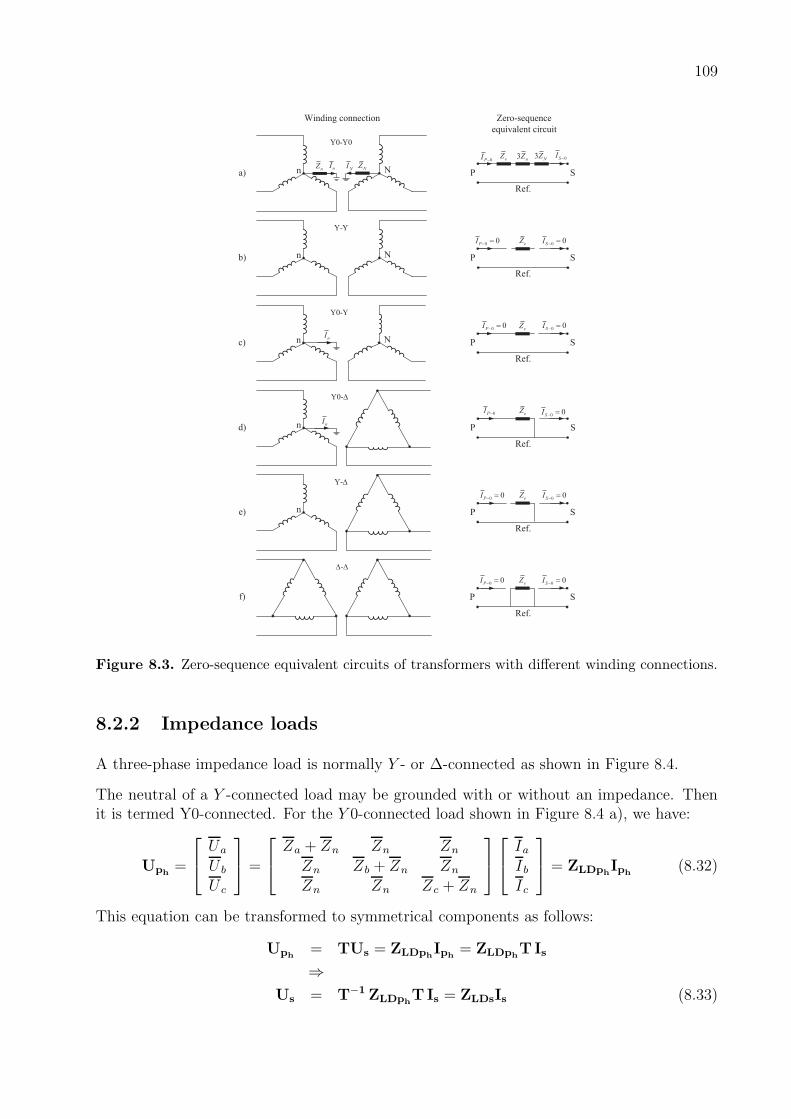
109
n nZ nI
n nI
NNZNI
Winding connection
a)
Y0-Y0
Zero-sequence
equivalent circuit
Ref.
SP
3 NZ3 nZeZ
Y0-
d)
n Nb)
Y-Y
SP
eZ
n Nc)
Y0-Y
Ref.
SP
eZ
nI
Ref.
SP
eZ
n
Y-
e)
Ref.
SP
eZ
-
f)
0PI 0SI
Ref.
0 0PI 0 0SI
0 0PI 0 0SI
0 0SI0PI
0 0SI0 0PI
Ref.
SP
eZ 0 0SI0 0PI
Figure 8.3. Zero-sequence equivalent circuits of transformers with different winding connections.
8.2.2 Impedance loads
A three-phase impedance load is normally Y - or ∆-connected as shown in Figure 8.4.
The neutral of a Y -connected load may be grounded with or without an impedance. Thenit is termed Y0-connected. For the Y 0-connected load shown in Figure 8.4 a), we have:
Uph=
Ua
U b
U c
=
Za + Zn Zn Zn
Zn Zb + Zn Zn
Zn Zn Zc + Zn
IaIbIc
= ZLDphIph
(8.32)
This equation can be transformed to symmetrical components as follows:
Uph= TUs = ZLDph
Iph= ZLDph
TIs
⇒Us = T−1ZLDph
TIs = ZLDsIs (8.33)

110
a) Y0-connected load
nZ
aZaIaU
bZbIbU
cZcI
cU
a b cI I I+ +
b) -connected load
abZ
aIaU
bcZ
bIbU acZ
cI
cU
Figure 8.4. Two possible load configurations
where
ZLDs ≡ T−1ZLDphT = (8.34)
=1
3
Za + Zb + Zc Za + α2Zb + αZc Za + αZb + α2Zc
Za + αZb + α2Zc Za + Zb + Zc Za + α2Zb + αZc
Za + α2Zb + αZc Za + αZb + α2Zc Za + Zb + Zc + 9Zn
As indicated in this matrix, there are non-diagonal elements that are nonzero, i.e. thereexists couplings between the positive-, negative- and zero-sequences. A special case is whenZa = Zb = Zc. In this special case, ZLDs can be written as
ZLDs =
Za 0 0
0 Za 00 0 Za + 3Zn
(8.35)
For a symmetric Y 0-connected load ZLD−1 = ZLD−2 = Za and ZLD−0 = Za + 3Zn. IfZn = 0 then ZLD−1 = ZLD−2 = ZLD−0. However, if the neutral of the load is not grounded,i.e a Y -connected load, then Zn = ∞ = ZLD−0 which means that no zero-sequence currentscan flow.
For the ∆-connected load shown in Figure 8.4 b), the impedance can be ∆-Y transformedwhich results in a Y -connected load:
Za =ZabZac
Zab + Zac + Zbc
(8.36)
Zb =ZabZbc
Zab + Zac + Zbc
(8.37)
Zc =ZacZbc
Zab + Zac + Zbc
(8.38)
Zn = ∞ (8.39)
For a symmetric ∆-connected load, i.e. Zab = Zbc = Zac, the symmetrical components canbe calculated by using equations (8.35) to (8.39) :
ZLD−1 = Zab/3 (8.40)
ZLD−2 = Zab/3 (8.41)
ZLD−0 = ∞ (8.42)

111
8.2.3 Transmission line
Series impedance of single-phase overhead line
The theory of having an overhead line using the ground as a return conductor was discussedby Carson in 1923. Carson considered a single conductor of unity length (e.g. one meter) inparallel with the ground, see Figure 8.5.
a
+
−a
U
+
−
Local earth
Ref.
Surface of
remote earth
0d
U =
d d ′Fictitious ground
return conductor
a′aaZ
ddZ
aI
d aI I= −
adD
adZ
1 Unit
Figure 8.5. Carson’s single-phase overhead line using the ground as return path
The current Ia flows in the conductor using the ground between d− d′ as return path. Theground is assumed to have an uniform resistance and an infinite extension. The current Id(=−Ia) is distributed over a large area, flowing along the ways of least resistance. Kirchhoff’slaw about the same voltage drop along each path is fulfilled. It has been shown that thesedistributed return paths may, in the analysis, be replaced by a single return conductor havinga radius εd located at a distance Dad from the overhead line according to Figure 8.5. Thedistance Dad is a function of the resistivity of the ground ρ. The distance Dad increases asthe resistivity ρ increases.
The inductance of this circuit can be calculated as
La =µ
2πln
1
Da︸ ︷︷ ︸
Laa
+µ
2πln
1
Dd︸ ︷︷ ︸
Ldd
−2µ
2πln
1
Dad︸ ︷︷ ︸
Lad
=µ
2π
(
lnDad
Da+ ln
Dad
Dd
)
(8.43)
where
µ = the permeability of the conductor
Da = e−1/4εa for a single conductor with radius εa
Dd = e−1/4εd for a return conductor in ground with radius εd
The inductance can according to equation (8.43) be divided into three parts, two apparent selfinductances (Laa, Ldd) and one apparent mutual inductance (Lad). Note that these quantitiesare only mathematical quantities without any physical meaning. For instance, they do nothave correct unit inside the ln-sign. It is only after the summation they achieve a physicalmeaning. Hopefully, the different part expressions will simplify the understanding of thebehavior of a three-phase line. The total series reactance of this single-phase conductor is
Xa = ωLa = ω(Laa + Ldd − 2Lad) (8.44)

112
By using this line model, having apparent inductances, the voltage drop for a single-phaseline can be calculated as
[Uaa′
Udd′
]
=
[Ua − Ua′
Ud − Ud′
]
=
[zaa zadzad zdd
] [Ia−Ia
]
V/length unit (8.45)
where Ua, Ua′ , Ud and Ud′ are given in proportion to the same reference. Since Ud = 0 andUa′ − Ud′ = 0, Ua can be obtained by subtracting the two equations from each other :
Ua = (zaa + zdd − 2zad)Ia = ZaIa (8.46)
By definitionZa ≡ zaa + zdd − 2zad Ω/length unit (8.47)
The impedances in this equation can be calculated as
zaa = ra + jxaa = ra + jωLaa Ω/length unit
zdd = rd + jxdd = rd + jωLdd Ω/length unit (8.48)
zad = jxad = jωLad Ω/length unit
Za = ra + rd + jXa Ω/length unit
where
ra = conductor resistance per length unit
rd = ground resistance per length unit
Series impedance of a three-phase overhead line
In order to obtain the series impedance of a three-phase line, the calculations are performedin the same way as for the single-phase line. In Figure 8.6, the impedances, voltages andcurrents of the line are given.
Since all conductors are grounded at a′, b′, c′, the following are valid
Ua′ − Ud′ =0 , U b′ − Ud′ = 0 , U c′ − Ud′ = 0
Id = − (Ia + Ib + Ic)(8.49)
The voltage drop over the conductors can be calculated as
Uaa′
U bb′
U cc′
Udd′
=
Ua − Ua′
U b − U b′
U c − U c′
Ud − Ud′
=
zaa zab zac zadzab zbb zbc zbdzac zbc zcc zcdzad zbd zcd zdd
IaIbIcId
V/length unit (8.50)
In a similar way as for the single-phase conductor, the impedances in equation (8.50) areapparent without any physical relevance. With Ud = 0 and by using equation (8.49), thefourth row can be subtracted from the first row in equation (8.50) which gives
Ua − (Ua′ − Ud′) = (zaa − 2zad + zdd)Ia + (zab − zad − zbd + zdd)Ib +
+ (zac − zad − zcd + zdd)Ic (8.51)

113
All wires grounded
here to local earth
potential
adZ
ddZdI
a aI
d
+
−
Ref.
0dU =
ccZc cI
aaZ
bbZb bI
d ′
c′
a′
b′
1 Unit
cU
aU
bU
bdZ
cdZ
abZ
bcZ
acZ
Figure 8.6. Three-phase overhead line with ground as return path
This can be simplified to Ua = ZaaIa+ZabIb+ZacIc. The impedances Zaa, Zab and Zac aredefined below. Note that when Ib = Ic = 0, the impedance Zaa is exactly the impedanceof a single-phase line using the ground as return path as described in section 8.2.3. If thecalculations above are repeated for the phases b and c, the following can be obtained
Ua
U b
U c
=
Zaa Zab Zac
Zab Zbb Zbc
Zac Zbc Zcc
IaIbIc
V/length unit (8.52)
where
Zaa = zaa − 2zad + zdd Ω/length unit
Zbb = zbb − 2zbd + zdd Ω/length unit
Zcc = zcc − 2zcd + zdd Ω/length unit (8.53)
Zab = Zba = zab − zad − zbd + zdd Ω/length unit
Zbc = Zcb = zbc − zbd − zcd + zdd Ω/length unit
Zac = Zca = zac − zad − zcd + zdd Ω/length unit
The impedances can be calculated in a similar way as shown in equations (8.43) and (8.48).It is important to concern the coupling between the phases. A current flowing in one phasewill influence the voltage drop in other phases. The replacing of a three-phase line withthree parallel impedances, is an approximation which gives that all non-diagonal element ofthe Z-bus matrix in equation (8.52) are neglected. In other words, the mutual inductancebetween the conductors are neglected. The error this simplification gives is dependent onseveral things, e.g. the distance between the conductors, the length of the conductors andthe magnitude of the currents in the conductors.

114
Symmetrical components of the series impedance of a three-phase line
Symmetrical components are often used in the analysis of power systems having three-phaselines, in order to simplify the complicated cross-couplings that exist between the phases.The quantities in equation (8.52) can be defined as :
Ua
U b
U c
= Uph= Zph
Iph=
Zaa Zab Zac
Zab Zbb Zbc
Zac Zbc Zcc
IaIbIc
(8.54)
The voltage vector (Uph) and current vector (Iph
) can be replaced by the correspondingsymmetrical component multiplied with matrix T according to the section on symmetricalcomponents :
Uph= TUs = Zph
TIs = ZphIph
(8.55)
This equation can be rewritten as
Us = T−1ZphTIs = ZsIs (8.56)
If a symmetrical overhead line (or cable) is assumed, i.e. Zaa = Zbb = Zcc and Zab = Zbc =Zac, the following is obtained
Zs = T−1ZphT =
1
3
1 α α2
1 α2 α1 1 1
Zaa Zab Zac
Zab Zbb Zbc
Zac Zbc Zcc
1 1 1α2 α 1α α2 1
=
=
Zaa − Zab 0 0
0 Zaa − Zab 00 0 Zaa + 2Zab
(8.57)
Equation (8.56) can be rewritten as
U−1
U−2
U−0
= Us = Zs Is = (8.58)
=
Zaa − Zab 0 00 Zaa − Zab 00 0 Zaa + 2Zab
I−1
I−2
I−0
=
Z−1 I−1
Z−2 I−2
Z−0 I−0
where
Z−1 = Zaa − Zab = positive-sequence impedance
Z−2 = Zaa − Zab = negative-sequence impedance (8.59)
Z−0 = Zaa + 2Zab = zero-sequence impedance
By inserting the expressions used in equation (8.53) into equation (8.59), the following canbe obtained
Z−1 = Z−2 = zaa − zab (8.60)
Z−0 = zaa + 2zab − 6zad + 3zdd

115
Note that the coupling to ground are not present in the expressions for the positive- andnegative-sequence impedances, i.e. the elements having index d in the Z-bus matrix inequation (8.50) are not included. This means that the zero-sequence current is zero in thepositive- and negative-sequence reference frame, which is quite logical. All couplings toground are represented in the zero-sequence impedance. As indicated above, a line by usingthis model, can be represented as three non-coupled components : positive-, negative-, andzero-sequence components. It should be pointed out that some loss of information will occurwhen using this model. For example, if only positive-, negative-, and zero-sequence data aregiven, the potential of the ground, Ud′ in Figure 8.6, cannot be calculated. To calculate thatpotential, more detailed data are needed. The line model introduced in subsection 6.1.2, isbased on positive-sequence data only, since symmetrical conditions are assumed.
Equivalent diagram of the series impedance of a line
As given above, for a symmetrical line Z−1 = Z−2. Assume that this line can be replaced byan equivalent circuit according to Figure 8.7, i.e. three phase impedances Zα and one return
aI aU ′
bU ′
cU ′
0U ′
aU
bU
cU
0U
bI
cI
0IZβ
Zα
Zα
Zα
Figure 8.7. Equivalent diagram of the series impedance of a line
impedance Zβ where the mutual inductance between the phases is assumed zero. With threephases and one return path, as given by the equivalent in Figure 8.7, the following is valid
I0 = Ia + Ib + Ic (8.61)
By using equation (8.61), the voltage drop between the phases and the return conductor canbe calculated as
U′a − U
′0 = Ua − U 0 − Ia · Zα − (Ia + Ib + Ic)Zβ
U′b − U
′0 = U b − U0 − Ib · Zα − (Ia + Ib + Ic)Zβ (8.62)
U′c − U
′0 = U c − U 0 − Ic · Zα − (Ia + Ib + Ic)Zβ
which can be rewritten to matrix form
U′a − U
′0
U′b − U
′0
U′c − U
′0
=
Ua − U0
U b − U 0
U c − U 0
−
Zα + Zβ Zβ Zβ
Zβ Zα + Zβ Zβ
Zβ Zβ Zα + Zβ
IaIbIc
(8.63)

116
or
U′ph
= Uph− ZαβIph
(8.64)
Since the matrix Zαβ is both symmetric and cyclo-symmetric, it can represent a line accordingto the assumption made. The matrix Zαβ can be converted to symmetrical components byusing equation (8.57) :
Zsαβ = T−1ZαβT =
Zα 0 00 Zα 00 0 Zα + 3Zβ
(8.65)
When the symmetrical components Z1 = Z2 and Z0 for the line are known, the following isobtained
Zα = Z−1
Zβ = Z−0−Z−1
3
(8.66)
With these values of Zα and Zβ, the equivalent in Figure 8.7 can be used, together withequation (8.63), to calculate the voltage drop between the phases and the return conductor(= Uph
−U′ph) as a function of the phase currents (= Iph
).
Note that the equivalent cannot be used to calculate e.g. U′0 −U 0 or U
′a −Ua but only e.g.
(U′a − U
′0)− (Ua − U0).
Example 8.3 Solve Example 2.5 by using symmetrical components.
LZ
aI aU ′
bU ′
cU ′
0U ′
aU
bU
cU
0U
bI
cI
0I
LZ
0LZ
aZ
bZ
cZ
LZ
Figure 8.8. Network diagram of the system in Example 8.3
Solution
According to the solutions in Example 2.5, the impedances of interest are ZL = 2.3 + j0.16Ω, ZL0 = 2.3 + j0.03 Ω, Za = 47.9 + j4.81 Ω, Zb = 15.97 + j1.60 Ω, Zc = 23.96+j2.40 Ω.
The symmetrical components of the line will first be calculated. Note that the line in theexample is given in the same way as the equivalent. The symmetrical components can becalculated by using equation (8.65) :
Z−1 = Z−2 = ZL = 2.3 + j0.16 ΩZ−0 = ZL + 3ZL0 = 9.2 + j0.25 Ω
(8.67)

117
which gives that
Zs =
Z−1 0 00 Z−2 00 0 Z−0
=
2.3 + j0.16 0 00 2.3 + j0.16 00 0 9.2 + j0.25
(8.68)
The symmetrical components for the load can be calculated by using equation (8.57)
ZLDs =1
3
1 α α2
1 α2 α1 1 1
Za 0 00 Zb 00 0 Zc
1 1 1α2 α 1α α2 1
=
=
29.28 + j2.94 9.09 + j3.24 9.55− j1.379.55− j1.37 29.28 + j2.94 9.09 + j3.249.09 + j3.24 9.55− j1.37 29.28 + j2.94
Ω (8.69)
The applied voltage is symmetric, i.e. it has only one sequence, the positive one :
Us = T−1Uph=
220 6 0
00
V (8.70)
The equation for this un-symmetric three-phase network can be described as
Us = (Zs + ZLDs)Is (8.71)
which can be rewritten as
Is = (Zs + ZLDs)−1Us =
8.11 6 − 5.51
2.22 6 149.09
1.75 6 − 155.89
A (8.72)
The symmetrical components for the voltage at the load can be calculated as
ULDs = ZLDsIs =
201.32 6 − 0.14
5.13 6 − 26.93
16.10 6 25.67
V (8.73)
The power obtained in the radiators can be calculated by using equation (8.24)
S = 3UtLDsI
∗s = 4754 + j477 VA (8.74)
i.e. the thermal power is 4754 W.
As given above, only the voltage drop at the load and the load currents can be calculated byusing the symmetrical components. The ground potential at the load cannot be calculated,but that is usually of no interest.
Previously, in Example 2.5, 4.1 and 4.2, the ground potential at the load has been calculatedby using other types of circuit analyses. It should be pointed out that the value of the groundpotential has no physical interpretation if the value of ZL and ZL0 has been obtained byusing the symmetrical components of the line according to equation (8.66). As given bythe solutions, the load demand, phase voltages at the load and the currents at the load arephysically correct by using either one of the four methods of solution.

118
Shunt capacitance of a three-phase line
The line resistance and inductance are components that together form the series impedanceof the line. The capacitance that is of interest in this section, forms the shunt component.
The series component, usually the inductance, gives a limit on the maximum amount of thecurrent that can be transmitted over the line, and by that also the maximum power limit.The capacitive shunt component behaves as a reactive power source. The reactive powergenerated, is proportional to the voltage squared, which implies that the importance of theshunt capacitance increases with the voltage level. For lines having a nominal voltage of300–500 kV and a length of more than 200 km, these capacitances are of great importance.In high voltage cables where the conductors are more close to one another, the capacitanceis up to 20–40 times larger than for overhead lines. The reactive power generation can be aproblem in cables having a length of only 10 km.
There is a fundamental law about electric fields saying that the electric potential v at acertain point on the distance d from a point charge q, can be calculated as :
v =q
4πǫ0dV (8.75)
where ǫ0 = 8.854× 10⁻¹² F/m, permittivity of vacuum. This law gives that there is a directrelationship between the difference in potential and accumulation of charges. If two long,parallel conductors are of interest, and if there is a voltage difference, v1 − v2, between thelines, an accumulation of charges with different sign, +Q and −Q, will take place. Themagnitude of the total charge Q depends mainly on the distance between the lines but alsoon the design of the lines. For cables, the material between the conductors will also have aninfluence on the charge accumulation. The capacitance between the two conductors is equalto the quotient between the charge Q and the difference in potential :
C ≡ Q
v1 − v2(8.76)
For a three-phase line, the corresponding capacitance is located between all conductors.When having a difference in potential between a conductor and ground, an accumulation ofcharges will also occur in relation to the magnitude of the capacitance. In Figure 8.9, thedifferent capacitances of a three-phase overhead line are given. A line is normally constructedin a symmetrical way, i.e. the mean distance between the phases are equal. Also, themean distance between a phase and ground is the same for all phases. In Figure 8.9, thiscorresponds to the case that cab = cbc = cac and cag = cbg = ccg when the entire line is ofinterest.
In the same way as given earlier for the series impedances, the positive-, negative- andzero-sequence capacitances can be calculated. Only the results from the calculations will bepresented here.
C−1 = C−2 =2πǫ0
ln[2HaAreq
] F/m (8.77)
C−0 =2πǫ0
ln[2HA2
reqa2
] F/m (8.78)

119
b
bccabc
acc
agc bgc cgc
c
a
Figure 8.9. Capacitances of a three-phase overhead line without earth wires
where, according to Figure 8.10
C−1 = positive-sequence capacitance
C−2 = negative-sequence capacitance
C−0 = zero-sequence capacitance
H = 3√
H1H2H3
A = 3√
A1A2A3
a = 3√a12a13a23
req = the equivalent radius of the line = e−1/4 × real radius of the line
Ground level
H1
H2 H
3
a12
a23
a13
A1
A2
A3
Figure 8.10. Geometrical quantities of a line in the calculation of capacitance
Note that C1 is equal to C2, but C0 has a different value. When having a closer lookat the equations for C1, it can be seen that 2H/A ≈ 1 according to Figure 8.10, whichmeans that the distance to ground has a relatively small influence. If the conductors arelocated close to one another, then 2H = A. The line model described in section 6.1.2, usesonly the positive-sequence capacitance C1 for the line. In principle, this can be regardedas a ∆-Y-transformation of the capacitances between the phases since they are the main

120
contributors to the positive- and negative-sequence capacitances. The coupling to ground isof less importance. In cables, the positive- and negative-sequence capacitances are usuallyhigher owing to the short distance between the phases.
For C−0, the coupling to ground is very important. When calculating C−0, all phases havethe same potential by the definition of zero-sequence. This implies that the capacitancesbetween the phases cab, cbc, cac are not of interest. However, the electric field is changedsince all three conductors have the same potential. As given in the equation, the distanceto ground is very important (power of three inside the ln-sign) in the calculations of thezero-sequence capacitance.
8.3 Analysis of unbalanced three-phase systems
As discussed in section 8.2, lines and transformers can be represented by their positive-, negative- and zero-sequence impedances. These sequences are decoupled which impliesthat for instance a certain zero-sequence current will only cause a zero-sequence voltagedrop whereas positive- and negative-sequence voltages will be unchanged. Also three-phasegenerators can in an equivalent way be described by decoupled positive-, negative- and zero-sequence systems.
This property implies that the entire system including generators, lines and transformerscan be represented by three decoupled systems.
8.3.1 Connection to a system under unbalanced conditions
In subsection 6.1.3, the connection to a network under symmetrical (or balanced) conditionswas discussed. It has been shown that by applying the Thevenin theorem the entire linearbalanced system (as seen from a selected point) can be represented by a voltage sourcebehind an impedance. The value of the impedance can be calculated when knowing thethree-phase short circuit current at the selected point.
A balanced power system as seen from a selected point p can be described by three de-coupled single-line sequence systems (or networks) termed as positive-, negative and zero-sequence systems. The model of the positive-sequence system is indeed the single-line systemof a balanced three-phase system that has been studied in chapters 5-6, i.e. in these chapterswe have studied the positive-sequence system of a balanced three-phase system.
Assuming a linear balanced three-phase power system, the sequence systems can be repre-sented by their Thevenin equivalents as shown in Figure 8.11. Note that there are no voltagesources in the network for the negative- and zero-sequence systems. Thus, the negative- andzero-sequence systems only consist of impedances.
From Figure 8.11, the following can be obtained in pu:
U p−1 = UThp − ZThp−1 Ip−1
U p−2 = 0− ZThp−2 Ip−2 (8.79)
U p−0 = 0− ZThp−0 Ip−0

121
~
1ThpZ −
ThpU
1pI −
a) Positive-sequence
2ThpZ −
2pI −
b) Negative-sequence
0ThpZ −
0pI −
c) Zero-sequence
1pU − 2pU − 0pU −
p p p
Figure 8.11. Thevenin equivalents as seen from a selected point p in the system.
8.3.2 Single line-to-ground fault
Assume that a single line-to-ground fault through an impedance Zf occurs at a point p inthe system, as shown in Figure 8.12.
faI
p
fZPhase a
0fbI =
0fcI =
Phase b
Phase c
Three-phase power system
Figure 8.12. Single-phase short circuit in phase a
Based on equation (8.11) the following is obtained:
Is =
Ip−1
Ip−2
Ip−0
=1
3
1 α α2
1 α2 α1 1 1
Ifa00
=1
3
IfaIfaIfa
⇒ Ip−1 = Ip−2 = Ip−0 =1
3Ifa (8.80)
From Figure 8.12, we have U pa = ZfIfa.
Using the first row in equation (8.14) and equations (8.79)-(8.80), the following is obtainedin pu:
Upa =Up−1 + U p−2 + U p−0 = ZfIfa = 3ZfIp−1 ⇒Upa =UThp − ZThp−1 Ip−1 − ZThp−2 Ip−1 − ZThp−0 Ip−1 = 3ZfIp−1 pu
(8.81)
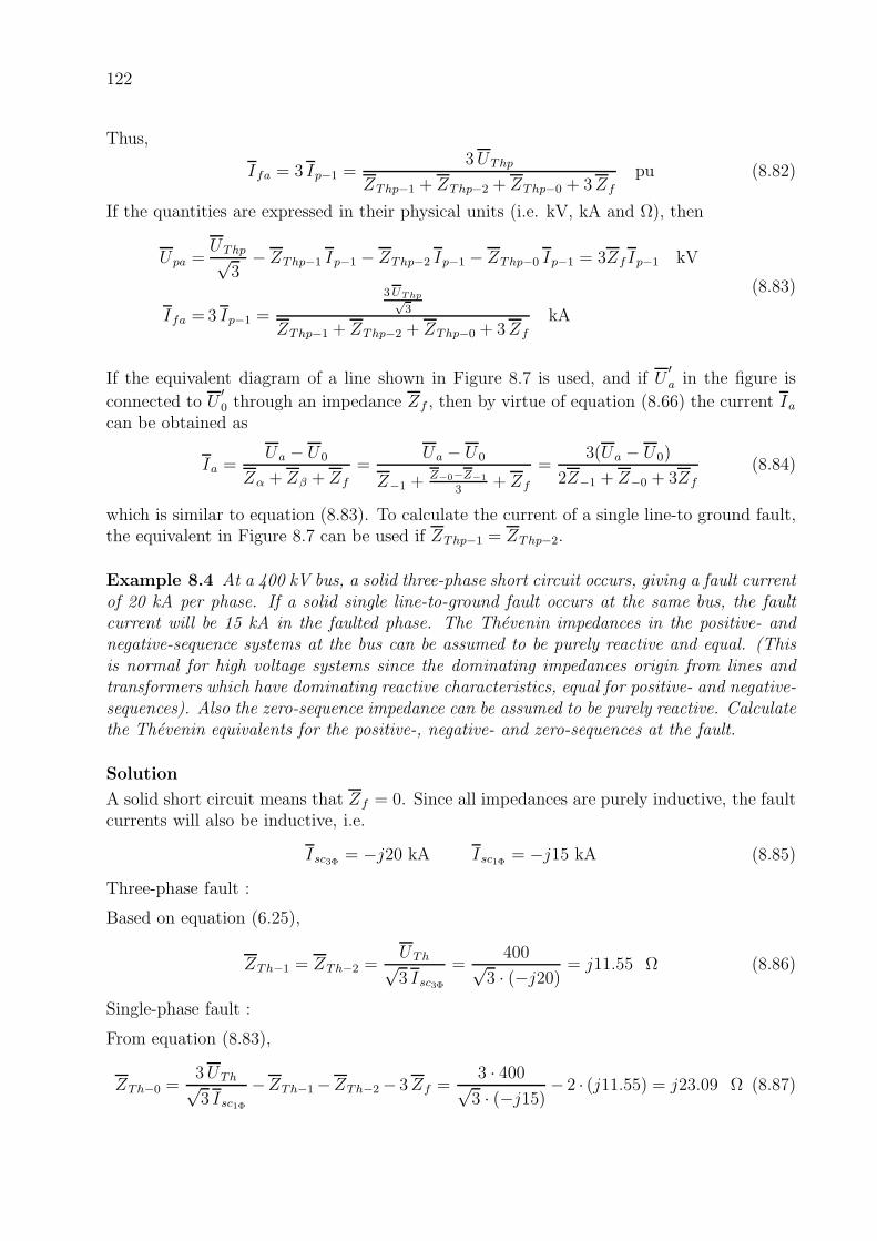
122
Thus,
Ifa = 3 Ip−1 =3UThp
ZThp−1 + ZThp−2 + ZThp−0 + 3Zf
pu (8.82)
If the quantities are expressed in their physical units (i.e. kV, kA and Ω), then
Upa =UThp√
3− ZThp−1 Ip−1 − ZThp−2 Ip−1 − ZThp−0 Ip−1 = 3ZfIp−1 kV
Ifa =3 Ip−1 =
3UThp√3
ZThp−1 + ZThp−2 + ZThp−0 + 3Zf
kA
(8.83)
If the equivalent diagram of a line shown in Figure 8.7 is used, and if U′a in the figure is
connected to U′0 through an impedance Zf , then by virtue of equation (8.66) the current Ia
can be obtained as
Ia =Ua − U 0
Zα + Zβ + Zf
=Ua − U 0
Z−1 +Z−0−Z−1
3+ Zf
=3(Ua − U0)
2Z−1 + Z−0 + 3Zf
(8.84)
which is similar to equation (8.83). To calculate the current of a single line-to ground fault,the equivalent in Figure 8.7 can be used if ZThp−1 = ZThp−2.
Example 8.4 At a 400 kV bus, a solid three-phase short circuit occurs, giving a fault currentof 20 kA per phase. If a solid single line-to-ground fault occurs at the same bus, the faultcurrent will be 15 kA in the faulted phase. The Thevenin impedances in the positive- andnegative-sequence systems at the bus can be assumed to be purely reactive and equal. (Thisis normal for high voltage systems since the dominating impedances origin from lines andtransformers which have dominating reactive characteristics, equal for positive- and negative-sequences). Also the zero-sequence impedance can be assumed to be purely reactive. Calculatethe Thevenin equivalents for the positive-, negative- and zero-sequences at the fault.
Solution
A solid short circuit means that Zf = 0. Since all impedances are purely inductive, the faultcurrents will also be inductive, i.e.
Isc3Φ = −j20 kA Isc1Φ = −j15 kA (8.85)
Three-phase fault :
Based on equation (6.25),
ZTh−1 = ZTh−2 =UTh√3 Isc3Φ
=400√
3 · (−j20)= j11.55 Ω (8.86)
Single-phase fault :
From equation (8.83),
ZTh−0 =3UTh√3 Isc1Φ
−ZTh−1−ZTh−2− 3Zf =3 · 400√3 · (−j15)
− 2 · (j11.55) = j23.09 Ω (8.87)

123
8.3.3 Analysis of a linear three-phase system with one unbalancedload
As discussed in subsection 8.3.1, the three sequence systems are decoupled when having abalanced system. However, in the case having unsymmetrical loads, these three sequencesystems will not be decoupled.
Assume a linear power system with an unbalanced load. The system is composed of a voltagesource, lines and transformers. This system can be analyzed as follows:
1. Draw the impedance diagrams of the positive-, negative and zero-sequence systems,for the entire network excluding the unbalanced load.
2. Find the Thevenin equivalents of the positive-, negative- and zero-sequence systems asseen from the point the unsymmetrical load is located.
3. Calculate the positive-, negative- and zero-sequence currents through the unbalancedload.
4. Calculate the positive-, negative- and zero-sequence voltages at the points of interest.
5. Calculate the positive-, negative- and zero-sequence currents through components thatare of interest.
6. Transform those symmetrical components to the phase quantities that are asked for.
The abovementioned points can be treated in different ways which will be shown in thefollowing example.
Example 8.5 Consider again the system described in Example 6.2. The following additionaldata is also given:
• Transformer is ∆-Y0 connected with Y 0 on the 10 kV-side, and Zn = 0.
• The zero-sequence impedance of the line is 3 times the positive-sequence impedance,i.e. Z21−0 = 3Z21−1.
• The zero-sequence shunt admittance of the line is 0.5 times the positive-sequence shuntadmittance, i.e. ysh−21−0 = 0.5 ysh−21−1.
• When the transformer is disconnected from bus 3, a solid (i.e. Zf = 0) single line-to-ground applied to this bus results in a pure inductive fault current of 0.2 kA.
• The positive- and negative-sequence Thevenin impedances of the power system are iden-tical, i.e. ZTh−1 = ZTh−2.
• The load is Y0-connected with Zn = 0. Furthermore, half of the normal load connectedto phase a is disconnected while the other phases are loaded as normal, i.e. it is anunsymmetrical load.

124
Calculate the voltage at the industry as well as the power fed by the transformer into theline.
Solution
1) Start with the building of the impedance diagram of the positive-, negative- and zero-sequence for the whole system excluding the unsymmetrical load, see Figure 8.13.
Positive- and negative-sequence components in per-unit values (from thesolution to Example 6.2):
1ThZ −
ThU
~21 1Z −1tZ −
123
4
power system
21 1shy − − 21 1shy − −
a) Positive-sequence system
2ThZ − 21 2Z −2tZ −
123
power system
21 2shy − − 21 2shy − −
b) Negative-sequence system
0ThZ − 21 0Z −0tZ −
12
power system
21 0shy − − 21 0shy − −
c) Zero-sequence system
4
4
3
Figure 8.13. Positive-, negative- and zero-sequence systems.

125
UTh =UThpu = 1 6 0
ZTh−1 =ZTh−2 = ZThpu = j 0.0137
Zt−1 =Zt−2 = Ztpu = j 0.004
Z21−1 =Z21−2 = Z21pu = 0.0225 + j 0.0075
ysh−21−1 = ysh−21−2 = ysh−21pu =j 0.003
2AL−1 =AL−2 = AL , BL−1 = BL−2 = BL
CL−1 =CL−2 = CL , DL−1 = DL−2 = DL
A−1 =A−2 = A , B−1 = B−2 = B
C−1 =C−2 = C , D−1 = D−2 = D
(8.88)
Zero-sequence components in per-unit values:
Isc1Φ =0.2 6 − 90
Ib70=
0.2 6 − 90
0.00412= 48.5437 6 − 90
ZTh−0 =3UTh
Isc1Φ− 2ZTh−1 − 0 = j 0.0344
Zt−0 =Zt−1 = j 0.004 , since Zn = 0
Z21−0 =3Z21−1 = 0.0675 + j 0.0225
ysh−21−0 =0.5 ysh−21−1 =j 0.003
4AL−0 =1 + ysh−21−0 · Z21−0 = 1.0000 + j 0.0001
BL−0 =Z21−0 = 0.0675 + j 0.0225
CL−0 = ysh−21−0(2 + ysh−21−0 · Z21−0) = 0.0000 + j 0.0015
DL−0 =AL−0 = 1.0000 + j 0.0001
(8.89)
2) Next step is to replace the networks with Thevenin equivalents as seen from the in-dustry connection point (bus 1), i.e. UThbus1, ZThbus1−1, ZThbus1−2 and ZThbus1−0, seeFigure 8.11.
The twoport of the entire positive-sequence network between bus 4 (which representsthe voltage source) and bus 1 (the industry connection point) is given by (see alsoExample 6.2):
[UTh
Ibus4−1
]
=
[A−1 B−1
C−1 D−1
] [U bus1−1
Ibus1−1
]
= (8.90)
=
[0.9999 + j0.0000 0.0225 + j0.02520.0000 + j0.0030 1.0000 + j0.0000
] [U bus1−1
Ibus1−1
]
Based on Figure 8.11 a), UThbus1−1 is obtained by setting Ibus1−1 = 0 as follows:
UTh =A−1 UThbus1−1 +B−1 · 0 ⇒
UThbus1−1 =UTh
A−1
= 1.0001 6 − 0.0019(8.91)

126
The Thevenin impedance ZThbus1−1 is obtained by setting UTh = 0 as follows:
0 = A−1 U bus1−1 +B−1 Ibus1−1 ⇒
ZThbus1−1 = − U bus1−1
Ibus1−1
=B−1
A−1
= 0.0225 + j0.0252(8.92)
To set UTh = 0, it means that bus 4 is short circuited. Therefore in this case, thepositive-sequence system will have a configuration similar to the negative-sequencesystem as shown in Figure 8.11 b). Furthermore, since Zt−1 = Zt−2, Z12−1 = Z12−2
and ysh−21−1 = ysh−21−2, they imply that A−1 = A−2 and B−1 = B−2. Thus, in asimilar way as shown in equation (8.92), the Thevenin impedance ZThbus1−2 is obtainedas follows:
0 = A−2 U bus1−2 +B−2 Ibus1−2 ⇒
ZThbus1−2 = − U bus1−2
Ibus1−2
=B−2
A−2
=B−1
A−1
= ZThbus1−1 = 0.0225 + j0.0252(8.93)
Based on Figure 8.3 d), the zero-sequence of a ∆-Y0-transformer should be modeledas an impedance to ground on the Y 0-side, as shown in Figure 8.13 c). As seen in thefigure, the feeding network (i.e. power system) is not connected to the industry loadfrom a zero-sequence point of view. The twoport of the network from the transformer(bus 3) to the connection point of the industry (bus 1) is given by
[U bus3−0
Ibus3−0
]
=
[0
Ibus3−0
]
=
[1 Zt−0
0 1
] [AL−0 BL−0
CL−0 DL−0
] [U bus1−0
Ibus1−0
]
=
=
[A−0 B−0
C−0 D−0
] [U bus1−0
Ibus1−0
]
= (8.94)
=
[1.0000 + j0.0001 0.0675 + j0.02650.0000 + j0.0015 1.0000 + j0.0001
] [U bus1−0
Ibus1−0
]
The Thevenin impedance ZThbus1−0 is obtained as follows:
0 =A−0 U bus1−0 +B−0 Ibus1−0 ⇒
ZThbus1−0 = − U bus1−0
Ibus1−0
=B−0
A−0
= 0.0675 + j0.0265(8.95)
3) From Example 6.2 the per-unit value of the load (i.e. ZLD) is known. At the half loadin phase a (i.e. ZLDa = 2ZLD), the impedance matrix of the symmetrical componentsis calculated based on equation (8.34) :
ZLDs =T−1 ZLDphT = T−1
2ZLD 0 0
0 ZLD 00 0 ZLD
T
=
1.0667 + j0.8000 0.2667 + j0.2000 0.2667 + j0.20000.2667 + j0.2000 1.0667 + j0.8000 0.2667 + j0.20000.2667 + j0.2000 0.2667 + j0.2000 1.0667 + j0.8000
(8.96)
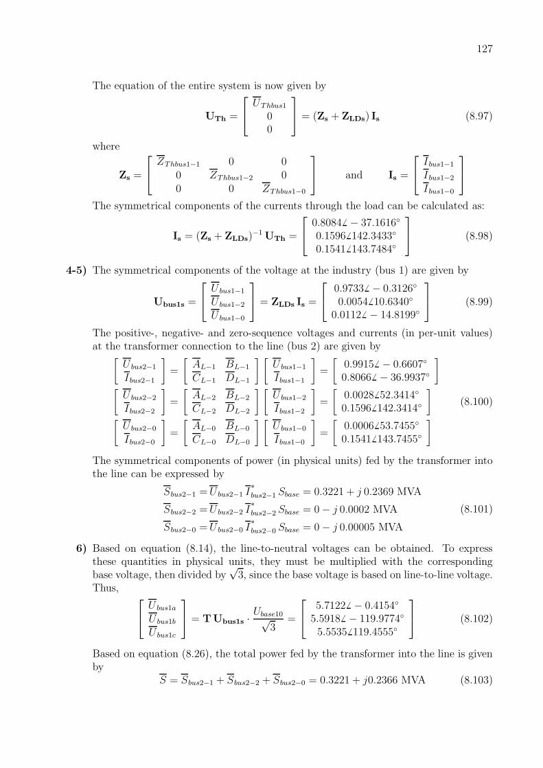
127
The equation of the entire system is now given by
UTh =
UThbus1
00
= (Zs + ZLDs) Is (8.97)
where
Zs =
ZThbus1−1 0 00 ZThbus1−2 00 0 ZThbus1−0
and Is =
Ibus1−1
Ibus1−2
Ibus1−0
The symmetrical components of the currents through the load can be calculated as:
Is = (Zs + ZLDs)−1UTh =
0.8084 6 − 37.1616
0.1596 6 142.3433
0.1541 6 143.7484
(8.98)
4-5) The symmetrical components of the voltage at the industry (bus 1) are given by
Ubus1s =
U bus1−1
U bus1−2
U bus1−0
= ZLDs Is =
0.9733 6 − 0.3126
0.0054 6 10.6340
0.0112 6 − 14.8199
(8.99)
The positive-, negative- and zero-sequence voltages and currents (in per-unit values)at the transformer connection to the line (bus 2) are given by
[U bus2−1
Ibus2−1
]
=
[AL−1 BL−1
CL−1 DL−1
] [U bus1−1
Ibus1−1
]
=
[0.9915 6 − 0.6607
0.8066 6 − 36.9937
]
[U bus2−2
Ibus2−2
]
=
[AL−2 BL−2
CL−2 DL−2
] [U bus1−2
Ibus1−2
]
=
[0.0028 6 52.3414
0.1596 6 142.3414
]
[U bus2−0
Ibus2−0
]
=
[AL−0 BL−0
CL−0 DL−0
] [U bus1−0
Ibus1−0
]
=
[0.0006 6 53.7455
0.1541 6 143.7455
]
(8.100)
The symmetrical components of power (in physical units) fed by the transformer intothe line can be expressed by
Sbus2−1 =U bus2−1 I∗bus2−1 Sbase = 0.3221 + j 0.2369 MVA
Sbus2−2 =U bus2−2 I∗bus2−2 Sbase = 0− j 0.0002 MVA
Sbus2−0 =U bus2−0 I∗bus2−0 Sbase = 0− j 0.00005 MVA
(8.101)
6) Based on equation (8.14), the line-to-neutral voltages can be obtained. To expressthese quantities in physical units, they must be multiplied with the correspondingbase voltage, then divided by
√3, since the base voltage is based on line-to-line voltage.
Thus,
U bus1a
U bus1b
U bus1c
= TUbus1s ·Ubase10√
3=
5.7122 6 − 0.4154
5.5918 6 − 119.9774
5.5535 6 119.4555
(8.102)
Based on equation (8.26), the total power fed by the transformer into the line is givenby
S = Sbus2−1 + Sbus2−2 + Sbus2−0 = 0.3221 + j0.2366 MVA (8.103)

128
8.4 A general method for analysis of linear three-phase
systems with one unbalanced load
In larger unsymmetrical systems, it is necessary to use a systematic approach to analyzesystem voltages and currents. In this section, all system components except one load, aresymmetrical. In the demonstration below, a small system is analyzed in the same way ascan be performed for a large system. The example given below is identical to the one insection 6.2 but with the difference that the load which will be connected to bus 2 is assumedunbalanced. The voltage source is represented by bus 3. All quantities are expressed inper-unit values.
Consider the simple balanced system shown in Figure 8.14. For a balanced system, all systemquantities and components can be represented only by their positive-sequence components.The only difference between this system and the system studied in section 6.2 is that herewe use index -1 which has been omitted in section 6.2.
~
1 1LDZ −
21 1Z −1tZ −
1233 1busI −
2 1busI − 1 1busI −
Figure 8.14. Single-phase impedance diagram of a symmetrical system.
The Y-bus matrix of the positive-sequence system is identical with Y in section 6.2, i.e.
Ibus1−1
Ibus2−1
Ibus3−1
= I1 = Y1U1 =
=
1ZLD1−1
+ 1Z12−1
− 1Z12−1
0
− 1Z21−1
1Z21−1
+ 1Zt−1
− 1Zt−1
0 − 1Zt−1
1Zt−1
U bus1−1
U bus2−1
U bus3−1
(8.104)
This Y-bus matrix can be inverted which results in the corresponding Z-bus matrix :
U1 = Y−11 I1 = Z1 I1 (8.105)
Since Ibus1−1 = Ibus2−1 = 0, the third row in equation (8.105) can be written as
U bus3−1 =Z1(3, 3) · Ibus3−1 ⇒
Ibus3−1 =U bus3−1
Z1(3, 3)
(8.106)

129
where Z1(3, 3) is an element in the Z-bus matrix. With this value of the current insertedinto equation (8.105) all voltages are obtained.
U bus1−1 = Z1(1, 3) · Ibus3−1 (8.107)
U bus2−1 = Z1(2, 3) · Ibus3−1 (8.108)
So far, all calculations are identical to those in section 6.2. Corresponding calculations canbe performed for an arbitrary large system having impedance loads and one voltagesource. Assume a system with a voltage source at bus i. The current at bus i and thevoltage at another bus r can then be calculated as:
Ibusi−1 =U busi−1
Z1(i, i)(8.109)
U busr−1 = UThbusr = Z1(r, i) · Ibusi−1 (8.110)
Now assume that an unsymmetrical impedance load is connected to bus 2 which apparentlyleads to the changes of the system voltages and currents. The actual voltages can be obtainedby using the theorem of superposition, i.e. as the sum of the voltages before the connection ofthe load and with the voltage change obtained by the load connection. This can be expressedby using symmetrical components as:
U′1 = Upre1 +U∆1
U′2 = Upre2 +U∆2 (8.111)
U′0 = Upre0 +U∆0
where, (below with all buses it means all buses in the system excluding the busconnected to the voltage source)
U′1 is a vector containing the positive-sequence voltages at all buses (i.e. bus 1 and bus 2
in this example) due to the connection of the unsymmetrical load.
U′2 is a vector containing the negative-sequence voltages at all buses due to the connection
of the unsymmetrical load.
U′0 is a vector containing the zero-sequence voltages at all buses due to the connection of
the unsymmetrical load.
Upre1 is a vector containing the positive-sequence voltages at all buses prior to the connec-tion of the unsymmetrical load.
Upre2 is a vector containing the negative-sequence voltages at all buses prior to the connec-tion of the unsymmetrical load. All elements of this vector are zero, since the systemis under balanced conditions prior to the connection of the unsymmetrical load.
Upre0 is a vector containing the zero-sequence voltages at all buses prior to the connectionof the unsymmetrical load. All elements of this vector are zero, since the system isunder balanced conditions prior to the connection of the unsymmetrical load.
U∆1 is a vector containing the changes in the positive-sequence voltages at all buses due tothe connection of the unsymmetrical load.

130
U∆2 is a vector containing the changes in the negative-sequence voltages at all buses dueto the connection of the unsymmetrical load.
U∆0 is a vector containing the changes in the zero-sequence voltages at all buses due to theconnection of the unsymmetrical load.
Equation (8.111) can be rewritten by expressing the voltage changes by a Z-bus matrixmultiplied with the current changes injected into the buses as follows:
U′1 = Upre1 + Z∆1 I∆1
U′2 = 0 + Z∆2 I∆2 (8.112)
U′0 = 0 + Z∆0 I∆0
where
Z∆1 is the Z-bus matrix of the positive-sequence system with the shortened voltage source.
Z∆2 is the Z-bus matrix of the negative-sequence system.
Z∆0 is the Z-bus matrix of the zero-sequence system.
I∆1 is a vector containing the injected positive-sequence current changes into the buses. Inthis example only I∆1(2) 6= 0, since the load is connected to bus 2.
I∆2 is a vector containing the injected negative-sequence current changes into the buses. Inthis example only I∆2(2) 6= 0.
I∆0 is a vector containing the injected zero-sequence current changes into the buses. In thisexample only I∆0(2) 6= 0.
Figure 8.15 shows the positive-, negative- and zero-sequence systems which will be used tocalculate the voltage changes due to connection of the unsymmetrical load at bus 2. Thedifference between the positive-sequence system in Figure 8.15 and the ∆-system used insection 6.2 is that the load is now represented by the currents injected into the buses. Theinfinite bus (bus 1) is assumed to be directly connected to ground and the transformer isY0-Y0 connected. The admittance matrices of the sequence networks shown in Figure 8.15can be formed as
Y∆1 =
[1
ZLD1−1+ 1
Z21−1− 1
Z21−1
− 1Z21−1
1Z21−1
+ 1Zt−1
]
Y∆2 =
[1
ZLD1−2+ 1
Z21−2− 1
Z21−2
− 1Z21−2
1Z21−2
+ 1Zt−2
]
(8.113)
Y∆0 =
[1
ZLD1−0+ 1
Z21−0− 1
Z21−0
− 1Z21−0
1Z21−0
+ 1Zt−0
]
Note that Y∆1 = Y1(1 : 2, 1 : 2), i.e. the row and column corresponding to the busconnected to the voltage source (bus 1 in this example) are removed, see also Y∆ in section

131
1 1LDZ −
21 1Z −1tZ −
123
1(2)I∆ 1(1) 0I∆ =
Positive-sequence
with shortened
voltage source
1 2LDZ −
21 2Z −2tZ −
123
2(2)I∆ 2(1)0I∆ =
Negative-sequence
1 0LDZ −
21 0Z −0tZ −
123
0(2)I∆ 0(1) 0I∆ =
Zero-sequence
Figure 8.15. Positive-, negative- and zero-sequence diagrams for calculations of thevoltage changes.
6.2. Furthermore, Y∆2 = Y∆1 for a system that is only composed of lines, transformers andsymmetrical impedance loads, since their positive- and negative-sequence components areidentical.
From the above Y-bus matrices the corresponding Z-bus matrices can be calculated as
Z∆1 = Y−1∆1
Z∆2 = Y−1∆2 (8.114)
Z∆0 = Y−1∆0
Since only the sequence components of the injected currents (i.e. I∆) into the bus to whichthe unsymmetrical load is connected (bus 2 in this example) are nonzero, these currents areof interest and will be calculated as follows. Based on equation (8.112), we have
U′bus2−1 = U′
1(2) = U bus2−1︸ ︷︷ ︸
from eq. (8.110)
+Z∆1(2, 2) I∆1(2)
U′bus2−2 = U′
2(2) = 0 + Z∆2(2, 2) I∆2(2) (8.115)
U′bus2−0 = U′
0(2) = 0 + Z∆0(2, 2) I∆0(2)
Assuming that the unsymmetrical load is connected to bus r (r = 2 in this example), theequations can be summarized as
U′s(r) =
U′busr−1
U′busr−2
U′busr−0
= Upre(r) + Z∆(r, r) I∆(r) = (8.116)
≡
UThbusr
00
+
Z∆1(r, r) 0 00 Z∆2(r, r) 00 0 Z∆0(r, r)
I∆1(r)I∆2(r)I∆0(r)

132
It should be pointed out that equation (8.116) indeed describes the Thevenin equivalentsas seen from bus r, where the voltage behind the positive-sequence impedance is UThbusr =U bus2−1 and the three Thevenin impedances are Z∆1(r, r), Z∆2(r, r) and Z∆0(r, r).
Assume that the unsymmetrical load is Y0-connected with ZLDbusra in phase a, ZLDbusrb inphase b and ZLDbusrc in phase c. The voltage drop over the load is
ULDbusrph=
ULDbusra
ULDbusrb
ULDbusrc
=
ZLDbusra 0 0
0 ZLDbusrb 00 0 ZLDbusrc
ILDbusra
ILDbusrb
ILDbusrc
=
= ZLDbusrphILDbusrph
(8.117)
By introducing symmetrical components, this can be converted to
U′s(r) =
U′busr−1
U′busr−2
U′busr−0
= T−1ULDbusrph
= T−1ZLDbusrphILDbusrph
=
= T−1ZLDbusrphT
︸ ︷︷ ︸
=ZLDbusrs
ILDbusrs = −ZLDbusrs I∆(r) (8.118)
Note that ILDbusrs is injected into the load, however I∆(r) is injected into the bus. Therefore,ILDbusrs = −I∆(r).
Next based on equations (8.116) and (8.118), the current I∆(r) can be expressed by
I∆(r) = − [Z∆(r, r) + ZLDbusrs]−1Upre(r) (8.119)
These values of the symmetrical components of the current at bus r can then be insertedinto equation (8.112) where the symmetrical components of all voltages can be calculated.The voltage at bus k can then be calculated as :
U′1(k) = Upre1(k) + Z∆1(k, r) I∆1(r)
U′2(k) = Z∆2(k, r) I∆2(r) (8.120)
U′0(k) = Z∆0(k, r) I∆0(r)
Example 8.6 Consider again the system described in Example 6.3. The following additionaldata is also given:
• The infinite bus (i.e. bus 1) has a grounded zero connection point.
• Transformer T1 is ∆-Y0 connected with Y 0 on the 10 kV-side, and Zn = 0.
• Transformer T2 is Y0-Y0 connected with Zn = 0.
• The zero-sequence impedances of the lines are 3 times the positive-sequence impedances,and the zero-sequence shunt admittances of the lines are 0.5 times the positive-sequenceshunt admittances.
• The load LD1 is ∆-connected.

133
• The load LD2 is Y0-connected with Zn = 0. Furthermore, half of the normal loadconnected to phase a is disconnected while the other phases are loaded as normal, i.e.LD2 is an unsymmetrical load.
Calculate the efficiency of the internal network operating in this unbalanced condition.Solution
1) Start with the building of the impedance diagram of the positive-, negative- and zero-sequence networks for the entire system excluding the unsymmetrical load, see Figure8.16.
1
2 3
4 5
1 1tZ −
23 1Z −
23 1shy − − 1 1LDZ −
24 1Z − 2 1tZ −
24 1shy − −
ThU
a) Positive-sequence system
1
2 3
4 5
1 2tZ −
23 2Z −
23 2shy − − 1 2LDZ −
24 2Z − 2 2tZ −
24 2shy − −
b) Negative-sequence system
1
2 3
4 5
1 0tZ −
23 0Z −
23 0shy − −
24 0Z − 2 0tZ −
24 0shy − −
c) Zero-sequence system
Figure 8.16. The sequence networks of the system in Example 8.6.
Positive- and negative-sequence components in per-unit values (from thesolution to Example 6.3):

134
UTh =U 1 = 1 6 0
Zt1−1 =Zt1−2 = Zt1pu = j 0.0438
Zt2−1 =Zt2−2 = Zt2pu = j 0.1333
Z23−1 =Z23−2 = Z23pu = 0.0017 + j 0.003
ysh−23−1 = ysh−23−2 = ysh−23pu =j 0.0013
2Z24−1 =Z24−2 = Z24pu = 0.0009 + j 0.0015
ysh−24−1 = ysh−24−2 = ysh−24pu =j 0.00064
2ZLD1−1 =ZLD1−2 = ZLD1pu = 0.64 + j 0.48
(8.121)
Zero-sequence components in per-unit values:
Zt1−0 =Zt1−1 = j 0.0438 , since Zn = 0
Zt2−0 =Zt2−1 = j 0.1333 , since Zn = 0
Z23−0 =3Z23−1 = 0.0051 + j 0.009
ysh−23−0 =0.5 ysh−23−1 =j 0.0013
4Z24−0 =3Z24−1 = 0.0026 + j 0.0045
ysh−24−0 =0.5 ysh−24−1 =j 0.00064
4ZLD1−0 =∞ , since ∆-connected
(8.122)
Next, the admittance matrix of the positive-sequence network (i.e. Y1) will be formedin a manner described in section 8.4. Bus 1 is included in order to determine thevoltage at all buses prior to the connection of the unsymmetrical load. However, theload LD2 is not included in the Y-bus matrix since it is unsymmetrical. It impliesthat Y1 is identical with the admittance matrix Y in Example 6.3 with the exceptionof the fifth diagonal element in which the unsymmetrical load LD2 is not included, i.e.Y1 = Y with Y 55 =
1Zt2−1
, see equation (6.49).
2) Next step is to replace the sequence networks with Thevenin equivalents as seen frombus 5, i.e. UThbus5, ZThbus5−1, ZThbus5−2 and ZThbus5−0, see Figure 8.11.
First, the Z-bus matrix is calculated as follows:
Z1 = Y−11 =
0.6429+j0.5264 0.6429+j0.4827 0.6412+j0.4797 0.6429+j0.4827 0.6429+j0.4827
0.6429+j0.4827 0.6429+j0.4827 0.6412+j0.4797 0.6429+j0.4827 0.6429+j0.4827
0.6412+j0.4797 0.6412+j0.4797 0.6412+j0.4797 0.6412+j0.4797 0.6412+j0.4797
0.6429+j0.4827 0.6429+j0.4827 0.6412+j0.4797 0.6437+j0.4842 0.6437+j0.4842
0.6429+j0.4827 0.6429+j0.4827 0.6412+j0.4797 0.6437+j0.4842 0.6437+j0.6175
Then, based on equation (8.110), the Thevenin voltage UThbus5 can be obtained as
UThbus5 = Z1(5, 1)Ibus1−1 = Z1(5, 1)UTh
Z1(1, 1)= 0.968 6 − 2.413 (8.123)

135
Based on equations (8.113)-(8.114), the positive-sequence impedance of the Theveninequivalent can be obtained from the Z-bus matrix of the positive-sequence systemwith voltage source shortened. This implies that in forming Y∆1, the row and columncorresponding to the bus connected to voltage source (i.e. bus 1) in matrix Y1 areremoved. Thus,
Y∆1 =
Y 22−1 − 1Z23−1
− 1Z24−1
0
− 1Z23−1
Y 33−1 0 0
− 1Z24−1
0 Y 44−1 − 1Zt2−1
0 0 − 1Zt2−1
1Zt2−1
(8.124)
The matrix Z∆1 can now be obtained as follows:
Z∆1 = Y−1∆1 =
0.0018+j0.0423 0.0018+j0.0421 0.0018+j0.0423 0.0018+j0.0423
0.0018+j0.0421 0.0036+j0.0449 0.0018+j0.0421 0.0018+j0.0421
0.0018+j0.0423 0.0018+j0.0421 0.0026+j0.0438 0.0026+j0.0438
0.0018+j0.0423 0.0018+j0.0421 0.0026+j0.0438 0.0026+j0.1771
(8.125)
Note that the element (4,4) corresponds to bus 5 since the row and column correspond-ing to bus 1 is removed. This implies that
ZThbus5−1 = 0.0026 + j0.1771 (8.126)
The Thevenin impedance of the negative-sequences ZThbus5−2 can be calculated usingthe corresponding matrix of the negative-sequence. The only difference between thepositive- and negative-sequence networks is that there is no voltage source in thenegative-sequence system.
Since all impedances (and thereby all admittances) in positive- and negative-sequencenetworks are identical, the following is valid
Y∆2 = Y∆1 (8.127)
Thus,ZThbus5−2 = ZThbus5−1 = 0.0026 + j0.1771 (8.128)
The Y-bus matrix of the zero-sequence is different compared with the other sequences,both owing to different numerical values but also because of the zero-sequence connec-tions in transformers and loads.
Y∆0 =
Y 22−0 − 1Z23−0
− 1Z24−0
0
− 1Z23−0
Y 33−0 0 0
− 1Z24−0
0 Y 44−0 − 1Zt2−0
0 0 − 1Zt2−0
1Zt2−0
(8.129)
where
Y 22−0 =1
Zt1−0
+1
Z23−0
+ ysh−23−0 +1
Z24−0
+ ysh−24−0
Y 33−0 =1
Z23−0
+ ysh−23−0
Y 44−0 =1
Z24−0
+ ysh−24−0 +1
Zt2−0

136
Corresponding Z-bus matrix is obtained as the inverse
Z∆0 = Y−1∆0 =
0.0000+j0.0438 0.0000+j0.0438 0.0000+j0.0438 0.0000+j0.0438
0.0000+j0.0438 0.0051+j0.0528 0.0000+j0.0438 0.0000+j0.0438
0.0000+j0.0438 0.0000+j0.0438 0.0026+j0.0483 0.0026+j0.0483
0.0000+j0.0438 0.0000+j0.0438 0.0026+j0.0483 0.0026+j0.1816
(8.130)
Note that element (4,4) corresponds to bus 5. Thus,
ZThbus5−0 = 0.0026 + j0.1816 (8.131)
Next, since all Thevenin equivalents as seen from bus 5 are identified, the voltage vectorand impedance matrix expressed in equation (8.116) can now be obtained as follows:
Upre(5) =
UThbus5
00
=
0.968 6 − 2.413
00
Z∆(5, 5) =
ZThbus5−1 0 00 ZThbus5−2 00 0 ZThbus5−0
= (8.132)
=
0.0026 + j0.1771 0 00 0.0026 + j0.1771 00 0 0.0026 + j0.1816
3) Determine the symmetrical components of the unsymmetrical load by using equation(8.118) and ZLD2pu from the solution to Example 6.3.
ZLDbus5s = T−1ZLDbus5phT = T−1
2ZLD2pu 0 00 ZLD2pu 00 0 ZLD2pu
T =
=
3.0083 + j0.9888 0.7521 + j0.2472 0.7521 + j0.24720.7521 + j0.2472 3.0083 + j0.9888 0.7521 + j0.24720.7521 + j0.2472 0.7521 + j0.2472 3.0083 + j0.9888
(8.133)
The symmetrical components of the currents through the load can now be determinedby using equations (8.119) and (8.132).
I∆(5) = − [Z∆(5, 5) + ZLDbus5s]−1Upre(5) =
0.3315 6 155.8442
0.0653 6 − 26.5244
0.0653 6 − 26.6221
=
I∆1(5)I∆2(5)I∆0(5)
(8.134)
4) The symmetrical components of all voltages can be calculated by using equations(8.110) and (8.120).

137
U′1(2) = Z1(2, 1) · Ibus1−1 + Z∆1(2, 5)I∆1(5) = 0.9618 6 − 3.1760
U′2(2) = Z∆2(2, 5)I∆2(5) = 0.0028 6 61.0623
U′0(2) = Z∆0(2, 5)I∆0(5) = 0.0029 6 63.3779
U′1(3) = Z1(3, 1) · Ibus1−1 + Z∆1(3, 5)I∆1(5) = 0.9581 6 − 3.2745
U′2(3) = Z∆2(3, 5)I∆2(5) = 0.0028 6 60.9638
U′0(3) = Z∆0(3, 5)I∆0(5) = 0.0029 6 63.3778 (8.135)
U′1(4) = Z1(4, 1) · Ibus1−1 + Z∆1(4, 5)I∆1(5) = 0.9614 6 − 3.1976
U′2(4) = Z∆2(4, 5)I∆2(5) = 0.0029 6 60.0356
U′0(4) = Z∆0(4, 5)I∆0(5) = 0.0032 6 60.3527
U′1(5) = Z1(5, 1) · Ibus1−1 + Z∆1(5, 5)I∆1(5) = 0.9465 6 − 5.6970
U′2(5) = Z∆2(5, 5)I∆2(5) = 0.0116 6 62.6242
U′0(5) = Z∆0(5, 5)I∆0(5) = 0.0119 6 62.5733
Note that the element numbers given in the above equations are the bus numbers.However, for Z∆ matrices, since the row and column corresponding to the bus con-nected to the voltage source (in this example bus 1) are removed, Z∆(k, r) correspondsto the element Z∆(k − 1, r − 1), i.e. with Z∆(2, 5) it means the element Z∆(1, 4).
Since Zt and ysh are lossless, the system losses are in the lines, i.e. Z23 and Z24. Thepositive-, negative- and zero-sequence currents through these impedances are expressedby
IZ23−1 =U′
1(2)−U′1(3)
Z23−1
= 1.1972 6 − 401209
IZ23−2 =U′
2(2)−U′2(3)
Z23−2
= 0.0034 6 − 24.1174
IZ23−0 =U′
0(2)−U′0(3)
Z23−0
= 0.0000 6 153.3778 (8.136)
IZ24−1 =U′
1(2)−U′1(4)
Z24−1
= 0.3314 6 − 24.1061
IZ24−2 =U′
2(2)−U′2(4)
Z24−2
= 0.0653 6 153.4756
IZ24−0 =U′
0(2)−U′0(4)
Z24−0
= 0.0653 6 153.3779
Positive-, negative- and zero-sequence powers injected into the line with impdance Z23
are given by
SZ23−1 = U′1(2)I
∗Z23−1 = 0.9203 + j0.6921
SZ23−2 = U′2(2)I
∗Z23−2 = (7.60 + j5.72)× 10−6 (8.137)
SZ23−0 = U′0(2)I
∗Z23−0 = 4.24× 10⁻¹⁵ + j2.61× 10−15

138
By using equation (8.25), the total power flowing through Z23 is given by
SZ23in = SZ23−1 + SZ23−2 + SZ23−0 = 0.4602 + j0.3461 (8.138)
In a similar manner, the following can also be obtained:
SZ24in = U′1(2)I
∗Z24−1 +U′
2(2)I∗Z24−2 +U′
0(2)I∗Z24−0 = 0.1489 + j0.0567
SZ23out = U′1(3)I
∗Z23−1 +U′
2(3)I∗Z23−2 +U′
0(3)I∗Z23−0 = 0.4589 + j0.3461
SZ24out = U′1(4)I
∗Z24−1 +U′
2(4)I∗Z24−2 +U′
0(4)I∗Z24−0 = 0.1488 + j0.0567
The efficiency can now be obtained as:
η = 100 · Real(SZ23out) +Real(SZ24out)
Real(SZ23in) +Real(SZ24in)= 99.7911% (8.139)
The efficiency can also be calculated as follows:
Sinj = U′1(2)
(UTh −U′
1(2)
Zt1−1
)∗
+U′2(2)
(0−U′
2(2)
Zt1−2
)∗+U′
0(2)
(0−U′
0(2)
Zt1−0
)∗
where, Sinj is the total power injected into the system by the infinite bus. Next, thetotal load is calculated as follows:
SLDtot=
|U′1(3)|2
Z∗LD1−1
+|U′
2(3)|2Z
∗LD1−2
+0+U′1(5)[−I∆1(5)]
∗+U′2(5)[−I∆2(5)]
∗+U′0(5)[−I∆0(5)]
∗
Thus,
η = 100 · Real(SLDtot)
Real(Sinj)% (8.140)
Note that (8.139) is valid if the losses are only in the lines. However, (8.140) is ageneral expression regardless of where the losses are.

Appendix A
Matlab-codes for Examples in Chapters 6-7
A.1 Example 6.2
clear
deg=180/pi;
rad=1/deg;
%--- Example 6.2
% Choose the base values
Sb=0.5; Ub10=10; Ib10=Sb/Ub10/sqrt(3);Zb10=Ub10^2/Sb;
Ub70=70; Ib70=Sb/Ub70/sqrt(3);
%Calculate the per-unit values of the Thevenin equivalent of the system
UTh=70*exp(j*0*rad);
Isc=0.3*exp(j*-90*rad);
UThpu =UTh/Ub70;
Iscpu =Isc/Ib70;
ZThpu =UThpu/Iscpu;
% Calculate the per-unit values of the transformer
Zt=j*4/100;Snt=5;
Ztpu=Zt*Sb/Snt;
%Calculate the per-unit values of the line
Z21pu=5*(0.9+j*0.3)/Zb10;
ysh21pu=5*(j*3*1E-6)*Zb10/2;
%Calculate the per-unit values of the industry impedance
cosphi=0.8;sinphi=sqrt(1-cosphi^2);
Un=Ub10;PLD=0.4;absSLD=PLD/cosphi;
SLD=absSLD*(cosphi+j*sinphi);
ZLDpu=Un^2/conj(SLD)/Zb10
% The twoport of the system
AL=1+ysh21pu*Z21pu;
BL=Z21pu;
CL=ysh21pu*(2+ysh21pu*Z21pu);
DL=AL;
F_L=[AL BL ; CL DL];
139
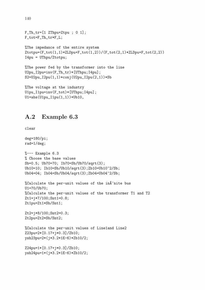
140
F_Th_tr=[1 ZThpu+Ztpu ; 0 1];
F_tot=F_Th_tr*F_L;
%The impedance of the entire system
Ztotpu=(F_tot(1,1)*ZLDpu+F_tot(1,2))/(F_tot(2,1)*ZLDpu+F_tot(2,2))
I4pu = UThpu/Ztotpu;
%The power fed by the transformer into the line
U2pu_I2pu=inv(F_Th_tr)*[UThpu;I4pu];
S2=U2pu_I2pu(1,1)*conj(U2pu_I2pu(2,1))*Sb
%The voltage at the industry
U1pu_I1pu=inv(F_tot)*[UThpu;I4pu];
U1=abs(U1pu_I1pu(1,1))*Ub10,
A.2 Example 6.3
clear
deg=180/pi;
rad=1/deg;
%--- Example 6.3
% Choose the base values
Sb=0.5; Ub70=70; Ib70=Sb/Ub70/sqrt(3);
Ub10=10; Ib10=Sb/Ub10/sqrt(3);Zb10=Ub10^2/Sb;
Ub04=04; Ib04=Sb/Ub04/sqrt(3);Zb04=Ub04^2/Sb;
%Calculate the per-unit values of the inA¯nite bus
U1=70/Ub70;
%Calculate the per-unit values of the transformer T1 and T2
Zt1=j*7/100;Snt1=0.8;
Zt1pu=Zt1*Sb/Snt1;
Zt2=j*8/100;Snt2=0.3;
Zt2pu=Zt2*Sb/Snt2;
%Calculate the per-unit values of Line1and Line2
Z23pu=2*[0.17+j*0.3]/Zb10;
ysh23pu=2*(j*3.2*1E-6)*Zb10/2;
Z24pu=1*[0.17+j*0.3]/Zb10;
ysh24pu=1*(j*3.2*1E-6)*Zb10/2;
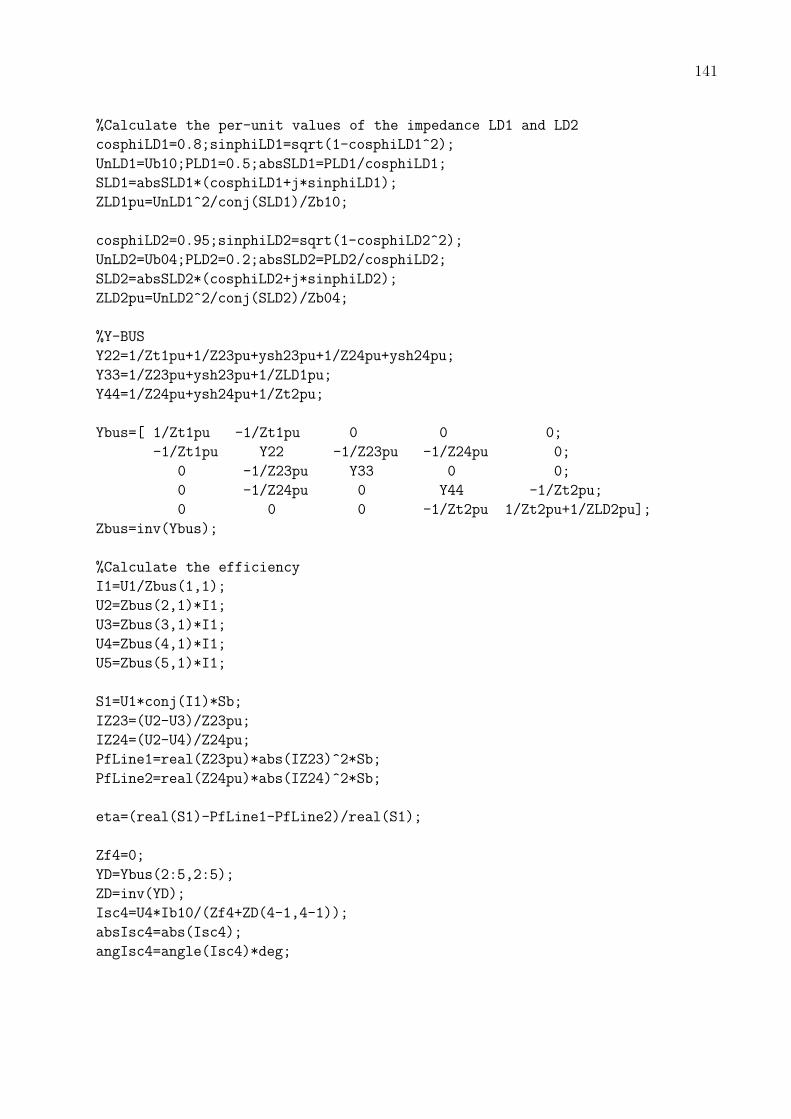
141
%Calculate the per-unit values of the impedance LD1 and LD2
cosphiLD1=0.8;sinphiLD1=sqrt(1-cosphiLD1^2);
UnLD1=Ub10;PLD1=0.5;absSLD1=PLD1/cosphiLD1;
SLD1=absSLD1*(cosphiLD1+j*sinphiLD1);
ZLD1pu=UnLD1^2/conj(SLD1)/Zb10;
cosphiLD2=0.95;sinphiLD2=sqrt(1-cosphiLD2^2);
UnLD2=Ub04;PLD2=0.2;absSLD2=PLD2/cosphiLD2;
SLD2=absSLD2*(cosphiLD2+j*sinphiLD2);
ZLD2pu=UnLD2^2/conj(SLD2)/Zb04;
%Y-BUS
Y22=1/Zt1pu+1/Z23pu+ysh23pu+1/Z24pu+ysh24pu;
Y33=1/Z23pu+ysh23pu+1/ZLD1pu;
Y44=1/Z24pu+ysh24pu+1/Zt2pu;
Ybus=[ 1/Zt1pu -1/Zt1pu 0 0 0;
-1/Zt1pu Y22 -1/Z23pu -1/Z24pu 0;
0 -1/Z23pu Y33 0 0;
0 -1/Z24pu 0 Y44 -1/Zt2pu;
0 0 0 -1/Zt2pu 1/Zt2pu+1/ZLD2pu];
Zbus=inv(Ybus);
%Calculate the efficiency
I1=U1/Zbus(1,1);
U2=Zbus(2,1)*I1;
U3=Zbus(3,1)*I1;
U4=Zbus(4,1)*I1;
U5=Zbus(5,1)*I1;
S1=U1*conj(I1)*Sb;
IZ23=(U2-U3)/Z23pu;
IZ24=(U2-U4)/Z24pu;
PfLine1=real(Z23pu)*abs(IZ23)^2*Sb;
PfLine2=real(Z24pu)*abs(IZ24)^2*Sb;
eta=(real(S1)-PfLine1-PfLine2)/real(S1);
Zf4=0;
YD=Ybus(2:5,2:5);
ZD=inv(YD);
Isc4=U4*Ib10/(Zf4+ZD(4-1,4-1));
absIsc4=abs(Isc4);
angIsc4=angle(Isc4)*deg;

142
A.3 Example 7.10
% Start of file
clear,
clear global
deg=180/pi;
maxiter=10;
EPS=1e-4;
k1=-0.2; k2=1.2; k3=-0.07; k4=0.4;
% Step 1
converged=0; iter=0; x=3/deg;
while ~converged & iter < maxiter,
% Step 2
delta_gx=k4-(k1*x+k2*cos(x-k3));
% Step Final
if all(abs(delta_gx)< EPS),
converged=1;
iter=iter,
xdeg=x*deg
else
% Step 3
Jac=k1-k2*sin(x-k3); %Jac=dfx/dx;
% Step 4
delta_x=inv(Jac)*delta_gx;
% Step 5
x=x+delta_x;
iter=iter+1;
end, % if all
if iter==maxiter,
iter=iter,
disp(’The equation has no solutions’)
disp(’or’)
disp(’bad initial value, try with another initial value’)
end, % iter
end, % while
% End of file

143
A.4 Example 7.12
% Start of file
clear,%
clear global
Sbase=100; Ubase=220; deg=180/pi;
%Step 1
% 1a)
U1=1;theta1=0;PLD1=0.2;QLD1=0.02;%
U2=1;PG2=1;PLD2=2;QLD2=0.2;
%1b)
Z12=0.02+j*0.2;%
Y=[1/Z12 -1/Z12 ; -1/Z12 1/Z12];%
G=real(Y); B=imag(Y);%
PGD2=PG2-PLD2;
%1c)
theta2=0;
iter=0;%
while iter < 3,
iter=iter+1;
%Step 2
%2a)
P2=U1*U2*(G(2,1)*cos(theta2-theta1)+B(2,1)*sin(theta2-theta1))+U2^2*G(2,2);
%2b
deltaP=PGD2-P2;
%Step 3
Q2=U2*U1*(G(2,1)*sin(theta2-theta1)-B(2,1)*cos(theta2-theta1))-U2^2*B(2,2);
H=-Q2-U2^2*B(2,2);
JAC=[H];
%Step 4
DX=inv(JAC)*[deltaP];
delta_theta2=DX;
%Step 5
theta2=theta2+delta_theta2;
end,
%Step final
P1=U1*U2*(G(1,2)*cos(theta1-theta2)+B(1,2)*sin(theta1-theta2))+U1^2*G(1,1);%
Q1=U1*U2*(G(1,2)*sin(theta1-theta2)-B(1,2)*cos(theta1-theta2))-U1^2*B(1,1);
Q2=U2*U1*(G(2,1)*sin(theta2-theta1)-B(2,1)*cos(theta2-theta1))-U2^2*B(2,2);
PG1=(P1+PLD1)*Sbase; QG1=(Q1+QLD1)*Sbase; QG2=(Q2+QLD2)*Sbase;
g=-G;b=-B;bsh_12=0;

144
P_12=(U1^2*g(1,2)-U1*U2*(g(1,2)*cos(theta1-theta2)+b(1,2)*sin(theta1-theta2)))*Sbase;
P_21=(U2^2*g(2,1)-U2*U1*(g(2,1)*cos(theta2-theta1)+b(2,1)*sin(theta2-theta1)))*Sbase;
Q_12=((-bsh_12-b(1,2))*U1^2-...
U1*U2*(g(1,2)*sin(theta1-theta2)-b(1,2)*cos(theta1-theta2)))*Sbase;
Q_21=((-bsh_12-b(2,1))*U2^2-...
U2*U1*(g(2,1)*sin(theta2-theta1)-b(2,1)*cos(theta2-theta1)))*Sbase;
PLoss=P_12+P_21; %or PLoss=(PG1+PG2)-(PLD1+PLD2)*Sbase;
ANG=[theta1 theta2]’*deg;
VOLT=[U1 U2]’*Ubase;
% End of file
A.5 Example 7.13
% Start of file
clear,%
clear global
tole=1e-6;
Sbase=100; Ubase=220; deg=180/pi;
%Step 1
% 1a)
U1=1;theta1=0;PLD1=0.2;QLD1=0.02;
PG2=1;QG2=0.405255;PLD2=2;QLD2=0.2;
%1b)
Z12=0.02+j*0.2;
Y=[1/Z12 -1/Z12 ; -1/Z12 1/Z12];
G=real(Y); B=imag(Y);
PGD2=PG2-PLD2;
QGD2=QG2-QLD2;
%1c)
theta2=0;
U2=1;
P2=U1*U2*(G(2,1)*cos(theta2-theta1)+B(2,1)*sin(theta2-theta1))+U2^2*G(2,2);
Q2=U2*U1*(G(2,1)*sin(theta2-theta1)-B(2,1)*cos(theta2-theta1))-U2^2*B(2,2);
deltaP=PGD2-P2;
deltaQ=QGD2-Q2;
%Step 3
while all(abs([deltaP;deltaQ])> tole),
H=-Q2-B(2,2)*U2^2;

145
N=P2+G(2,2)*U2^2;
J=P2-G(2,2)*U2^2;
L=Q2-B(2,2)*U2^2;
JAC=[H N ; J L];
%Step 4
DX=inv(JAC)*[deltaP;deltaQ];
%Step 5
theta2=theta2+DX(1); %DX(1)=delta_theta2
U2=U2*(1+DX(2)); %DX(2)=delta_U2/U2
%Step 2
P2=U1*U2*(G(2,1)*cos(theta2-theta1)+B(2,1)*sin(theta2-theta1))+U2^2*G(2,2);
Q2=U2*U1*(G(2,1)*sin(theta2-theta1)-B(2,1)*cos(theta2-theta1))-U2^2*B(2,2);
deltaP=PGD2-P2;
deltaQ=QGD2-Q2;
end, %while
%Step final
P1=U1*U2*(G(1,2)*cos(theta1-theta2)+B(1,2)*sin(theta1-theta2))+U1^2*G(1,1);%
Q1=U1*U2*(G(1,2)*sin(theta1-theta2)-B(1,2)*cos(theta1-theta2))-U1^2*B(1,1);
Q2=U2*U1*(G(2,1)*sin(theta2-theta1)-B(2,1)*cos(theta2-theta1))-U2^2*B(2,2);
PG1=(P1+PLD1)*Sbase; QG1=(Q1+QLD1)*Sbase; QG2=(Q2+QLD2)*Sbase;
g=-G;b=-B;bsh_12=0;
P_12=(U1^2*g(1,2)-U1*U2*(g(1,2)*cos(theta1-theta2)+b(1,2)*sin(theta1-theta2)))*Sbase;
P_21=(U2^2*g(2,1)-U2*U1*(g(2,1)*cos(theta2-theta1)+b(2,1)*sin(theta2-theta1)))*Sbase;
Q_12=((-bsh_12-b(1,2))*U1^2-...
U1*U2*(g(1,2)*sin(theta1-theta2)-b(1,2)*cos(theta1-theta2)))*Sbase;
Q_21=((-bsh_12-b(2,1))*U2^2-...
U2*U1*(g(2,1)*sin(theta2-theta1)-b(2,1)*cos(theta2-theta1)))*Sbase;
PLoss=P_12+P_21; %or PLoss=(PG1+PG2)-(PLD1+PLD2)*Sbase;
ANG=[theta1 theta2]’*deg;
VOLT=[U1 U2]’*Ubase;
% End of file
A.6 Example 7.14
% To run Load Flow (LF), two MATLAB-files are used, namely
% (run_LF.m) and (solve_lf.m)
% Start of file (run_LF.m)

146
clear%
clear global
%%%%%%%%%%%%%%%%%%%%%%%%%%
tole=1e-9; deg=180/pi; rad=1/deg ;
%%%%%%%%%%%%%%
% Base values
%%%%%%%%%%%%%%
Sbase=100; Ubase=220; Zb=Ubase^2/Sbase;
%%%%%%%%%%%%
% Bus data
%%%%%%%%%%%%
% Number of buses
nbus=4;
%Bus 1, slack bus
U1=220/Ubase; theta1=0*rad; PLD1=10/Sbase; QLD1=2/Sbase;
%Bus 2, PQ-bus
PG2=0/Sbase; QG2=0/Sbase; PLD2=90/Sbase; QLD2=10/Sbase;
%Bus 3, PQ-bus
PG3=0/Sbase; QG3=0/Sbase; PLD3=80/Sbase; QLD3=10/Sbase;
%Bus 4, PQ-bus
PG4=0/Sbase; QG4=0/Sbase; PLD4=50/Sbase; QLD4=10/Sbase;
%%%%%%%%%%%%
% Line data
%%%%%%%%%%%%
Z12=(5+j*65)/Zb;bsh12=0.0002*Zb;%
Z13=(4+j*60)/Zb;bsh13=0.0002*Zb;%
Z23=(5+j*68)/Zb;bsh23=0.0002*Zb;%
Z34=(3+j*30)/Zb;bsh34=0;
%%%%%%%%%%%%%%
% YBUS matrix
%%%%%%%%%%%%%%
y11=1/Z12+1/Z13+j*bsh12+j*bsh13; y12=-1/Z12; y13=-1/Z13; y14=0;%
y21=-1/Z12; y22=1/Z12+1/Z23+j*bsh12+j*bsh23; y23=-1/Z23; y24=0;%
y31=-1/Z13; y32=-1/Z23; y33=1/Z13+1/Z23+1/Z34+j*bsh13+j*bsh23; y34=-1/Z34;%
y41=0; y42=0; y43=-1/Z34; y44=1/Z34;%
YBUS=[ ];% Define YBUS
G=real(YBUS); B=imag(YBUS);
%%%%%%%%%%%%%%%%%%%%%%%%%%%%%%%%%%
% PGD for PU- and PQ-buses
%%%%%%%%%%%%%%%%%%%%%%%%%%%%%%%%%%
PGD2=PG2-PLD2; % for bus 2 (PQ-bus)
PGD3=PG3-PLD3; % for bus 3 (PQ-bus)
PGD4=PG4-PLD4; % for bus 4 (PQ-bus)
PGD=[PGD2 ; PGD3 ; PGD4];
%%%%%%%%%%%%%%%%%%%%%%%%%%

147
% Define the column vector QGD for PQ-buses
%%%%%%%%%%%%%%%%%%%%%%%%%%
QGD=[ ];
%%%%%%%%%%%%%%%%%%%%%%%%%%%%%%%%%%%%%%%%%%%%%%%%%
% Use fsolve function in MATLAB to run load flow
%%%%%%%%%%%%%%%%%%%%%%%%%%%%%%%%%%%%%%%%%%%%%%%%%
% Unknown variables [theta2 theta3 theta4 U2 U3 U4]’;
% Define the initial values of the unknown variables
X0=[0 0 0 1 1 1]’; % Flat initial values
s_z=size(X0);
nx=s_z(1,1); % number of unknown variables
% The function below is used for fsolve (type "help fsolve" in MATLAB)
options_solve=optimset(’Display’,’off’,’TolX’,tole,’TolFun’,tole);
% Parameters used for fsolve
PAR=[nx ; nbus ; U1 ; theta1];% U1 and theta1 are known (slack bus).
[X_X,FVAL,EXITFLAG,OUTPUT]=fsolve(’solve_lf’,X0,options_solve,G,B,PGD,QGD,PAR);
if EXITFLAG~=1,
disp(’No solution’),
EXITFLAG=EXITFLAG,
return
end,
% Solved variables X_X=[theta2 theta3 theta4 U2 U3 U4]’;
ANG=[theta1 X_X(1) X_X(2) X_X(3)]’;% Voltage phase angles
VOLT=[U1 X_X(4) X_X(5) X_X(6)]’; % Voltage magnitudes
ANG_deg=ANG*deg;% in degrees
VOLT_kV=VOLT*Ubase; % in kV
%%%%%%%%%%%%%%%%%%%%%%%%%%%%%%%%%%%%%%%%%%%%%%%%%%%%%%%%%%%%%%%%%%
% The generated active and reactive power at slack bus and PU-buses
%%%%%%%%%%%%%%%%%%%%%%%%%%%%%%%%%%%%%%%%%%%%%%%%%%%%%%%%%%%%%%%%%
g=-G;b=-B;
% At slack bus, bus 1
P12=g(1,2)*VOLT(1)^2-...
VOLT(1)*VOLT(2)*(g(1,2)*cos(ANG(1)-ANG(2))+b(1,2)*sin(ANG(1)-ANG(2)));
P13=g(1,3)*VOLT(1)^2-...
VOLT(1)*VOLT(3)*(g(1,3)*cos(ANG(1)-ANG(3))+b(1,3)*sin(ANG(1)-ANG(3)));
Q12=(-bsh12-b(1,2))*VOLT(1)^2-...
VOLT(1)*VOLT(2)*(g(1,2)*sin(ANG(1)-ANG(2))-b(1,2)*cos(ANG(1)-ANG(2)));
Q13=(-bsh13-b(1,3))*VOLT(1)^2-...
VOLT(1)*VOLT(3)*(g(1,3)*sin(ANG(1)-ANG(3))-b(1,3)*cos(ANG(1)-ANG(3)));%

148
PG1=P12+P13+PLD1;%
QG1=Q12+Q13+QLD1;%
% You may also use equation (7.43) (Pk and Qk) to find PG1 and QG1
PG1= ; % based on equation (7.43)
QG1= ; % based on equation (7.43)
PG1_MW=PG1*Sbase;%
QG1_MVAr=QG1*Sbase;
%%%%%%%%%%%%%%%%%%%%%%%%%%%%%%%%%
%%%%%%%%%
% Losses
%%%%%%%%%
PLoss_tot=(PG1+PG2+PG3+PG4)-(PLD1+PLD2+PLD3+PLD4);%
PLoss_tot_MW=PLoss_tot*Sbase;
PLoss_Sys1= ;% Find the power losses in System 1 (pu)
PLoss_Sys1_MW=PLoss_Sys1*Sbase;
PLoss_Sys2_MW= ; % Find the power losses in System 2 (MW)
% End of file (run_LF.m)
%%%%%%%%%%%%%%
% Second file
%%%%%%%%%%%%%%
% Start of file (solve_lf.m)
% This function solves g(x)=0 for x.
function [g_x]=solve_lf(X,G,B,PGD,QGD,PAR);
nx=PAR(1); nbus=PAR(2); U1=PAR(3); theta1=PAR(4);
PGD2=PGD(1); PGD3=PGD(2); PGD4=PGD(3); QGD2=QGD(1); QGD3=QGD(2); QGD4=QGD(3);
theta2=X(1); theta3=X(2); theta4=X(3); U2=X(4); U3=X(5); U4=X(6);
ANG=[theta1 theta2 theta3 theta4]’ ; VOLT=[U1 U2 U3 U4]’;
% We have nx unknown variables, therefore the
% size of g(x) is nx by 1.
g_x=zeros(nx,1);

149
%Based on equation (7.43), find Pk and Qk
P2= ;
P3= ;
P4= ;
Q2= ;
Q3= ;
Q4= ;
% Active power mismatch (PU- and PQ-buses)
% Bus 2
g_x(1)=P2-PGD2;
% Bus 3
g_x(2)=P3-PGD3;
% Bus 4
g_x(3)=P4-PGD4;
% Reactive power mismatch (PQ-buses)
% Bus 2
g_x(4)=Q2-QGD2;
% Bus 3
g_x(5)=Q3-QGD3;
% Bus 4
g_x(6)=Q4-QGD4;
% End of file (solve_lf.m)
A.7 Example 7.15
% Changes in file run_LF.m
%%%%%%%%%%%%
% Bus data
%%%%%%%%%%%%
% Number of buses
nbus=4;
%Bus 3, PU-bus
PG3=0/Sbase; U3=220/Ubase; PLD3=80/Sbase; QLD3=10/Sbase;
%%%%%%%%%%%%
% Line data
%%%%%%%%%%%%
%%%%%%%%%%%%%%

150
% YBUS matrix
%%%%%%%%%%%%%%
%%%%%%%%%%%%%%%%%%%%%%%%%%%%%%%%%%
% Define PGD for PU- and PQ-buses
%%%%%%%%%%%%%%%%%%%%%%%%%%%%%%%%%%
%%%%%%%%%%%%%%%%%%%%%%%%%%
% Define QGD for PQ-buses
%%%%%%%%%%%%%%%%%%%%%%%%%%
QGD2=QG2-QLD2; % for bus 2 (PQ-bus)
QGD4=QG4-QLD4; % for bus 4 (PQ-bus)
QGD=[QGD2 ; QGD4];
%%%%%%%%%%%%%%%%%%%%%%%%%%%%%%%%%%%%%%%%%%%%%%%%%
% Use fsolve function in MATLAB to run load flow
%%%%%%%%%%%%%%%%%%%%%%%%%%%%%%%%%%%%%%%%%%%%%%%%%
% Unknown variables [theta2 theta3 theta4 U2 U4]’;
% Define the initial values of the unknown variables
X0=[0 0 0 1 1]’; % Flat initial values
% Parameters used for fsolve
PAR=[nx ; nbus ; U1 ; U3 ; theta1];%
% Solved variables X_X=[theta1 theta2 theta4 U2 U4]’;
ANG=[theta1 X_X(1) X_X(2) X_X(3)]’;%
VOLT=[U1 X_X(4) U3 X_X(5)]’;
%%%%%%%%%%%%%%%%%%%%%%%%%%%%%%%%%%%%%%%%%%%%%%%%%%%%%%%%%%%%%%%%%%
% The generated active and reactive power at slack bus and PU-buses
%%%%%%%%%%%%%%%%%%%%%%%%%%%%%%%%%%%%%%%%%%%%%%%%%%%%%%%%%%%%%%%%%
g=-G;b=-B;
% At slack bus, bus 1
% At PU-buses, bus 3
QG3= ;%
QG3_MVAr=QG3*Sbase;
%%%%%%%%%
% Losses
%%%%%%%%%

151
% End of file (run_LF.m)
%%%%%%%%%%%%%%
% Second file
%%%%%%%%%%%%%%
% Start of file (solve_lf.m)
function [g_x]=solve_lf(X,G,B,PGD,QGD,PAR);
nx=PAR(1); nbus=PAR(2); U1=PAR(3); U3=PAR(4); theta1=PAR(5);
PGD2=PGD(1); PGD3=PGD(2); PGD4=PGD(3); QGD2=QGD(1); QGD4=QGD(2);
theta2=X(1); theta3=X(2); theta4=X(3); U2=X(4); U4=X(5);
ANG=[theta1 theta2 theta3 theta4]’; VOLT=[U1 U2 U3 U4]’;
% We have nx unknown variables, therefore the
% size of g(x) is nx by 1.
g_x=zeros(nx,1);
for m=1:nbus
for n=1:nbus
PP(m,n)=VOLT(m)*VOLT(n)*(G(m,n)*cos(ANG(m)-ANG(n))+B(m,n)*sin(ANG(m)-ANG(n)));
QQ(m,n)=VOLT(m)*VOLT(n)*(G(m,n)*sin(ANG(m)-ANG(n))-B(m,n)*cos(ANG(m)-ANG(n)));
end, %for n
end, % for m
P=sum(PP’)’;
Q=sum(QQ’)’;
% Active power mismatch (PU- and PQ-buses)
% Bus 2
g_x(1)=P(2)-PGD2;
% Bus 3
g_x(2)=P(3)-PGD3;
% Bus 4
g_x(3)=P(4)-PGD4;
% Reactive power mismatch (PQ-buses)
% Bus 2
g_x(4)=Q(2)-QGD2;
% Bus 4
g_x(5)=Q(4)-QGD4;
% End of file (solve_lf.m)

152
A.8 Example 8.5
clear
% 1) Start with the building of the impedance diagram of the positive-, negative-
% and zero-sequence for the whole system excluding the unsymmetrical load
Ex6_2, % Run Example 6.2
%Positive- and negative-sequence components in per-unit values (from the
%solution to Example 6.2):
UTh=UThpu;
ZTh_1=ZThpu;
ZTh_2=ZTh_1;
Zt_1=Ztpu;
Z21_1=Z21pu;
Z21_2=Z21_1;
ysh21_1=ysh21pu;
ysh21_2=ysh21_1;
AL_1=AL ; AL_2=AL_1;
BL_1=BL ; BL_2=BL_1;
CL_1=CL ; CL_2=CL_1;
DL_1=DL ; DL_2=DL_1;
A_1=F_tot(1,1) ; A_2=A_1;
B_1=F_tot(1,2) ; B_2=B_1;
C_1=F_tot(2,1) ; C_2=C_1;
D_1=F_tot(2,2) ; D_2=D_1;
%Zero-sequence components in per-unit values
Isc1phi=0.2*exp(-j*90*rad)/Ib70;
ZTh_0=3*UTh/Isc1phi-2*ZTh_1;
Zt_0=Zt_1;
Z21_0=3*Z21_1;
ysh21_0=0.5*ysh21_1;
AL_0=1+ysh21_0*Z21_0;
BL_0=Z21_0;
CL_0=ysh21_0*(2+ysh21_0*Z21_0);
DL_0=AL_0;
% 2) Next step is to replace the networks with Thevenin equivalents as seen
% from the industry connection point (bus 1)

153
UThbus1=UTh/A_1;%
ZThbus1_1=B_1/A_1;
ZThbus1_2=ZThbus1_1;
F_tot_0=[ 1 Zt_0 ; 0 1]*[AL_0 BL_0 ; CL_0 DL_0];
ZThbus1_0=F_tot_0(1,2)/F_tot_0(1,1);
% 3) Symmetrical components
alfa=exp(j*120*rad);
TT=[1 1 1 ; alfa^2 alfa 1 ; alfa alfa^2 1];
ZLDs=inv(TT)*[2*ZLDpu 0 0 ; 0 ZLDpu 0 ; 0 0 ZLDpu]*TT;
UTH=[UThbus1 ; 0 ; 0];
Zs=[ZThbus1_1 0 0 ; 0 ZThbus1_2 0 ; 0 0 ZThbus1_0];
Is=inv(Zs+ZLDs)*UTH;
% 4-5) The symmetrical components of the voltage at the industry (bus 1)
Ubus1s=ZLDs*Is;
Ubus2_Ibus2_1=[AL_1 BL_1 ; CL_1 DL_1]*[Ubus1s(1) ; Is(1)];
Ubus2_Ibus2_2=[AL_2 BL_2 ; CL_2 DL_2]*[Ubus1s(2) ; Is(2)];
Ubus2_Ibus2_0=[AL_0 BL_0 ; CL_0 DL_0]*[Ubus1s(3) ; Is(3)];
Sbus2_1=Ubus2_Ibus2_1(1,1)*conj(Ubus2_Ibus2_1(2,1))*Sb;
Sbus2_2=Ubus2_Ibus2_2(1,1)*conj(Ubus2_Ibus2_2(2,1))*Sb;
Sbus2_0=Ubus2_Ibus2_0(1,1)*conj(Ubus2_Ibus2_0(2,1))*Sb;
% 6)
Ubus1_Ph=[abs(TT*Ubus1s*Ub10/sqrt(3)) angle(TT*Ubus1s*Ub10/sqrt(3))*deg]
Stot=Sbus2_1+Sbus2_2+Sbus2_0
A.9 Example 8.6
clear,
Ex6_3,
% 1)
% Positive- and negative-sequence components in per-unit values (from the
% solution to Example 6.3)
UTh=U1;
Zt1_1=Zt1pu ; Zt1_2=Zt1_1;%
Zt2_1=Zt2pu ; Zt2_2=Zt2_1;%
Z23_1=Z23pu ; Z23_2=Z23_1;%
ysh23_1=ysh23pu ; ysh23_2=ysh23_1;%
Z24_1=Z24pu ; Z24_2=Z24_1;%
ysh24_1=ysh24pu ; ysh24_2=ysh24_1;%
ZLD1_1=ZLD1pu ; ZLD1_2=ZLD1_1;%

154
%Zero-sequence components in per-unit values
Zt1_0=Zt1_1 ; Zt2_0=Zt2_1;%
Z23_0=3*Z23_1 ; ysh23_0=0.5*ysh23_1;%
Z24_0=3*Z24_1 ; ysh24_0=0.5*ysh24_1;%
% 2)
Y1=Ybus; Y1(5,5)=1/Zt2_1; Z1=inv(Y1);
Ibus1_1=UTh/Z1(1,1);
UThbus5=Z1(5,1)*Ibus1_1;
YD1=Y1(2:5,2:5);
ZD1=inv(YD1);
ZD2=ZD1;
% 3)
ZThbus5_1=ZD1(5-1,5-1); ZThbus5_2=ZThbus5_1;
Y22_0=1/Zt1_0+1/Z23_0+ysh23_0+1/Z24_0+ysh24_0;
Y33_0=1/Z23_0+ysh23_0;
Y44_0=1/Z24_0+ysh24_0+1/Zt2_0;
YD0=[ Y22_0 -1/Z23_0 -1/Z24_0 0;
-1/Z23_0 Y33_0 0 0;
-1/Z24_0 0 Y44_0 -1/Zt2_0;
0 0 -1/Zt2_0 1/Zt2_0];
ZD0=inv(YD0);
ZThbus5_0=ZD0(5-1,5-1);
UPre_5=[UThbus5 ; 0 ; 0];
ZD_5=[ZThbus5_1 0 0 ; 0 ZThbus5_2 0 ; 0 0 ZThbus5_0];
alfa=exp(j*120*rad);
TT=[1 1 1 ; alfa^2 alfa 1 ; alfa alfa^2 1];
ZLDbus5s=inv(TT)*[2*ZLD2pu 0 0 ; 0 ZLD2pu 0 ; 0 0 ZLD2pu]*TT;
ID_5=-inv(ZD_5+ZLDbus5s)*UPre_5;
% 4)
Up2_1=Z1(2,1)*Ibus1_1+ ZD1(2-1,5-1)*ID_5(1);
Up2_2= 0 + ZD2(2-1,5-1)*ID_5(2);
Up2_0= 0 + ZD0(2-1,5-1)*ID_5(3);
Up3_1=Z1(3,1)*Ibus1_1+ ZD1(3-1,5-1)*ID_5(1);
Up3_2= 0 + ZD2(3-1,5-1)*ID_5(2);
Up3_0= 0 + ZD0(3-1,5-1)*ID_5(3);
Up4_1=Z1(4,1)*Ibus1_1+ ZD1(4-1,5-1)*ID_5(1);
Up4_2= 0 + ZD2(4-1,5-1)*ID_5(2);
Up4_0= 0 + ZD0(4-1,5-1)*ID_5(3);
Up5_1=Z1(5,1)*Ibus1_1+ ZD1(5-1,5-1)*ID_5(1);
Up5_2= 0 + ZD2(5-1,5-1)*ID_5(2);
Up5_0= 0 + ZD0(5-1,5-1)*ID_5(3);

155
IZ23_1=(Up2_1-Up3_1)/Z23_1;
IZ23_2=(Up2_2-Up3_2)/Z23_2;
IZ23_0=(Up2_0-Up3_0)/Z23_0;
IZ24_1=(Up2_1-Up4_1)/Z24_1;
IZ24_2=(Up2_2-Up4_2)/Z24_2;
IZ24_0=(Up2_0-Up4_0)/Z24_0;
SZ23_1=Up2_1*conj(IZ23_1);
SZ23_2=Up2_2*conj(IZ23_2);
SZ23_0=Up2_0*conj(IZ23_0);
SZ23_in=SZ23_1+SZ23_2+SZ23_0;
SZ24_in=Up2_1*conj(IZ24_1)+Up2_2*conj(IZ24_2)+Up2_0*conj(IZ24_0);
SZ23_out=Up3_1*conj(IZ23_1)+Up3_2*conj(IZ23_2)+Up3_0*conj(IZ23_0);
SZ24_out=Up4_1*conj(IZ24_1)+Up4_2*conj(IZ24_2)+Up4_0*conj(IZ24_0);
eta=100*(real(SZ23_out)+real(SZ24_out))/(real(SZ23_in)+real(SZ24_in))
Sinj=UTh*conj((UTh-Up2_1)/Zt1_1)+Up2_2*conj((0-Up2_2)/Zt1_2)+...
Up2_0*conj((0-Up2_0)/Zt1_0);
SLDtot=abs(Up3_1)^2/ZLD1_1+abs(Up3_2)^2/ZLD1_2+0-...
Up5_1*conj(ID_5(1))-Up5_2*conj(ID_5(2))-Up5_0*conj(ID_5(3));
eta=100*real(SLDtot)/real(Sinj)

156
Appendix B
Analysis of three-phase systems using lineartransformations
In this chapter, the possibilities of using linear transformations in order to simplify the anal-ysis of three-phase systems, are briefly discussed. These transformations are general and arevalid under both symmetrical and un-symmetrical conditions. By generalizing the expres-sions for a symmetric three-phase voltage given in equations (2.10) and (2.14), correspondingexpressions for an arbitrary three-phase voltage at constant frequency can be obtained as
ua(t) = UMa cos(ωt+ γa)ub(t) = UMb cos(ωt+ γb)uc(t) = UMc cos(ωt+ γc)
Ua = Ua 6 γa
U b = Ub 6 γb
U c = Uc 6 γc
(B.1)
where UMa, UMb, UMc are peak values, Ua, Ub, Uc are RMS-values and γa, γb, γc are phaseangles of the three voltages. For the un-symmetrical currents, corresponding expressionshold as
ia(t) = IMa cos(ωt+ γa − φa)ib(t) = IMb cos(ωt+ γb − φb)ic(t) = IMc cos(ωt+ γc − φc)
Ia = Ia 6 γa − φa
Ib = Ib 6 γb − φb
Ic = Ic 6 γc − φc
(B.2)
where IMa, IMb, IMc are peak values, Ia, Ib, Ic are RMS-values of the three phase currentswhereas φa, φb, φc are the phase of the currents in relation to the corresponding phasevoltage.
The mean value of the total three-phase active power can be calculated as
P3 =UMa√
2
IMa√2cosφa +
UMb√2
IMb√2cos φb +
UMc√2
IMc√2cosφc (B.3)
whereas the total three-phase complex power is
S3 = UaI∗a + U bI
∗b + U cI
∗c = (UaIa cosφa + UbIb cosφb + UcIc cosφc) +
+ j(UaIa sin φa + UbIb sinφb + UcIc sinφc) (B.4)
This phase representation is in many cases sufficient for a three-phase system analysis. Thereare a number of important cases when the analysis can greatly be simplified by using lineartransformations.
This chapter discusses the following items. First, the advantages of using linear transfor-mations in three-phase system analysis are generally discussed. Later on, some specifictransformations to be used in certain conditions are given. In order to really understandthe subject of transformations, the reader is referred to text books on the subject, e.g. inelectric machine theory or high power electronics. In chapter 8, one of the transformationsof interest, symmetrical components, is discussed in more detail. The purpose of chapter ??is to show that the idea and the mathematics behind the transformations are the same. Itis only the choice of linear transformation, i.e. transformation matrix, that is different.
157

158
B.1 Linear transformations
By using transformations, components are mapped from an original space (the original spaceis here the instantaneous values or the complex representation of the phase quantities) to animage space. A linear transformation means that the components in the image space are alinear combination of the original space. The complex values of the phase voltages can bemapped with a linear transformation as
UA = waaUa + wabU b + wacU c
UB = wbaUa + wbbU b + wbcU c (B.5)
UC = wcaUa + wcbU b + wccU c
which in matrix form can be written as
UA
UB
UC
=
waa wab wac
wba wbb wbc
wca wcb wcc
Ua
U b
U c
(B.6)
or in a more compact notation
UABC = WUabc (B.7)
The elements in matrix W are independent of the values of the original and image spacecomponents. In this example, the components in the original space Ua, U b and U c aremapped by using the linear transformation W to the image space components UA, UB andUC . The original space components can be calculated from the image space components byusing the inverse of matrix W (W−1 = T), i.e.
Uabc = W−1UABC = TUABC (B.8)
The only mappings that are of interest, are those where W−1 are existing. In the following,the matrix T or its inverse T−1 will represent the linear transformation.
B.1.1 Power invarians
A usual demand for the linear transformations in power system analysis is that it should bepossible to calculate the electric power in the image space by using the same expressions asin the original space and that the two spaces should give the same result. A transformationthat can meet that requirement is called power invariant. Using the complex representation,the electric power in the original space can be calculated by using equation (B.4), this gives
Sabc = UaI∗a + U bI
∗b + U cI
∗c = Ut
abc I∗abc (B.9)
where “t” indicates the transpose.In the image space, the corresponding expression is
SABC = UAI∗A + UBI
∗B + UCI
∗C = Ut
ABCI∗ABC (B.10)

159
Power invarians implies that SABC = Sabc, i.e.
UtABCI
∗ABC = Ut
abcI∗abc = (TUABC)
t(TIABC)∗ = Ut
ABCTtT∗I∗ABC (B.11)
This gives that the transformation matrix T must fulfill the following condition :
TtT∗ = ((T∗)t T)t = 1 =
1 0 00 1 00 0 1
(B.12)
which leads toT−1 = (T∗)t (B.13)
If T is real, equation (B.13) implies that T is an orthogonal matrix.
B.1.2 The coefficient matrix in the original space
Consider a three-phase line between two buses. The voltage drop Uabc over the line dependson the current Iabc flowing in the different phases. The voltage drop can be expressed as
Uabc =
Ua
U b
U c
=
Zaa Zab Zac
Zba Zbb Zbc
Zca Zcb Zcc
IaIbIc
= ZabcIabc (B.14)
where Zabc is the coefficient matrix of the line. Note that each element in Zabc is non-zerosince a current in one phase has influence on the voltage drop in the other phases owing tothe mutual inductance, see chapter 8.2.
Symmetrical matrices
A matrix that is symmetrical around its diagonal is called a symmetrical matrix (or moreprecisely, Hermitian if the matrix contains complex entries). For the Z-bus matrix in equation(B.14), this implies that Zab = Zba, Zac = Zca and Zbc = Zcb, i.e.
Zabc =
Zaa Zab Zac
Zab Zbb Zbc
Zac Zbc Zcc
= Ztabc (B.15)
An example of a symmetrical matrix is the one representing a line (or a cable) where thenon-diagonal element are dependent on the mutual inductance, which is equal between thephases a–b and the phases b–a, see chapter 8.2.
Cyclo-symmetrical matrices
The Z-bus matrix in equation (B.14) is cyclo-symmetric if Zab = Zbc = Zca, Zba = Zac = Zcb
and Zaa = Zbb = Zcc, i.e.
Zabc =
Zaa Zab Zba
Zba Zaa Zab
Zab Zba Zaa
(B.16)
160
All normal three-phase systems are cyclo-symmetrical, i.e. if ia, ib, ic are permuted to ib,ic, ia, the voltages ua, ub, uc will also be permuted to ub, uc, ua. This implies that ordinaryoverhead lines, cables, transformers and electrical machines can be represented by cyclo-symmetrical matrices.
B.1.3 The coefficient matrix in the image space
If both sides of equation (B.14) are multiplied with the matrix T−1, the following is obtained
UABC = T−1Uabc = T−1ZabcIabc = (T−1ZabcT)IABC = ZABCIABC (B.17)
whereZABC = T−1ZabcT (B.18)
ZABC is the image space mapping of the coefficient matrix Zabc. This gives that if UABC
represents the image space voltages, and IABC represents the image space currents thenZABC will represent the impedances in the image space.
One reason of introducing a linear transformation may be to obtain a diagonal coefficientmatrix in the image space, i.e.
ZABC =
ZAA 0 0
0 ZBB 00 0 ZCC
(B.19)
By having a diagonal coefficient matrix, equation (B.17) can be rewritten as
UA = ZAAIA
UB = ZBBIB (B.20)
UC = ZCCIC
i.e. the matrix equation (B.17) with mutual couplings between the phases is replaced bythree un-coupled equations. If ZABC is diagonal as in equation (B.19), both sides in equation(B.18) can be multiplied with T and rewritten as
TZABC =
T1 T2 T3
ZAA 0 00 ZBB 00 0 ZCC
=
ZAAT1 ZBBT2 ZCCT3
=
= ZabcT = Zabc
T1 T2 T3
(B.21)
where T1, T2, T3 are the columns of T. Equation (B.21) can be rewritten as
ZabcT1 − ZAAT1 = 0
ZabcT2 − ZBBT2 = 0 (B.22)
ZabcT3 − ZCCT3 = 0
161
i.e. ZAA, ZBB and ZCC are the eigenvalues of matrix Zabc and the vectors T1, T2 and T3
are the corresponding eigenvectors. A transformation that maps the matrix Z to a diagonalform should have a transformation matrix T having columns that are the eigenvectors of thematrix Z. Note that eigenvectors can be scaled arbitrarily.
B.2 Examples of linear transformations that are used
in analysis of three-phase systems
In the following, four commonly used linear transformations will be briefly introduced. Ingeneral, transformations can be presented in a little bit different way in different text books.It is therefore of importance to understand the definitions used by the authors.
B.2.1 Symmetrical components
In the analysis of un-symmetrical conditions in a power system, symmetrical componentsare commonly used. This complex, linear transformation uses the fact that all components(lines, machines, etc.) in normal systems are cyclo-symmetrical, i.e. their impedances canbe modeled by equation (B.16). The power invariant transformation matrix and its inversefor the symmetrical components are
TS =1√3
1 1 11 α2 α1 α α2
T−1S =
1√3
1 1 11 α α2
1 α2 α
(B.23)
where α = ej120
. As given by the definition T−1S = (T∗
S)t which corresponds to the assump-
tion of power invariant according to equation (B.13). By using this transformation, cyclo-symmetrical matrices are transformed into a diagonal form as given in equation (B.19), i.e.the columns of matrix TS consist of the eigenvectors to a cyclo-symmetrical matrix. Thiswill simplify the system analysis as indicated in equation (B.20). Using the given phasorvoltages Ua, U b and U c, the power invariant symmetrical components can be calculated as
Us =
U0
U1
U2
= T−1S Uabc =
1√3
1 1 11 α α2
1 α2 α
Ua
U b
U c
(B.24)
The three components U 0, U 1 and U 2 are called zero-sequence, positive-sequence and negative-sequence, respectively. A cyclo-symmetrical impedance matrix according to equation (B.16)can be diagonalized by using symmetrical components according to equation (B.18) as
ZS = T−1S
Zaa Zab Zba
Zba Zaa Zab
Zab Zba Zaa
TS =
Z0 0 00 Z1 00 0 Z2
(B.25)

162
where
Z0 = Zaa + Zab + Zba = zero-sequence impedance
Z1 = Zaa + α2Zab + αZba = positive-sequence impedance (B.26)
Z2 = Zaa + αZab + α2Zba = negative-sequence impedance
The three impedances Z0, Z1 and Z2 are the eigenvalues of the cyclo-symmetrical impedancematrix. For an impedance matrix that is both cyclo-symmetric and symmetric, i.e. Zba =Zab, the result after a diagonalization will be that
Z0 = Zaa + 2Zab
Z1 = Zaa − Zab (B.27)
Z2 = Zaa − Zab
Transformers, overhead lines, cables and symmetrical loads (not electrical machines) can benormally represented by impedance matrices that are both symmetrical and cyclo-symmetrical,i.e. all diagonal elements are equal and all non-diagonal elements are equal. This gives thatthe positive-sequence impedance and the negative-sequence impedance are equal.
In order to make the positive-sequence phasor voltage equal to the line-to-neutral phasorvoltage, a reference invariant form of transformation for the symmetrical components isnormally used. The reference invariant transformation matrix and its inverse are
TS′ =
1 1 11 α2 α1 α α2
=√3 ·TS T−1
S′ =1
3
1 1 11 α α2
1 α2 α
=1√3·T−1
S (B.28)
The reference invariant transformation is not power invariant since T−1S′ = 1
3(T∗
S′)t. The
name reference invariant means that in symmetrical conditions U1 = Ua. Note that trans-formations of coefficient matrices, according to equation (B.18), are not influenced whetherthe power invariant or the reference invariant matrix is used since
ZABC(eff − inv) = T−1S ZabcTS =
(1√3T−1
S
)
Zabc
(√3TS
)
=
= T−1S′ ZabcTS′ = ZABC(ref − inv) (B.29)
A third variation of the transformation matrix for the symmetrical components arises whenthe ordering of the sequences is changed. If the positive-sequence is given first and thezero-sequence last, the columns of the T-matrix and the rows in the T−1 are permuted,respectively. This results in the following reference invariant transformations matrices :
TS′′ =
1 1 1α2 α 1α α2 1
T−1S′′ =
1
3
1 α α2
1 α2 α1 1 1
(B.30)
This form of the transformation matrices will be used in chapter 8 where symmetrical com-ponents are discussed in more detail. The only thing that happens with the coefficient matrixin the image space is that the diagonal elements change places.
As described above, a number of different variations of the symmetrical components canbe used, all having the same fundamental purpose, to diagonalize the cyclo-symmetricalimpedance matrices.

163
B.2.2 Clarke’s components
Clarke’s components, also called α−β-components or orthogonal components, divides thosephase-quantities not having any zero-sequence into two orthogonal components. The wordzero-sequence means the same as when discussing symmetrical components, the sum of thephase components. Components that do not have zero-sequence are those whose sum is equalto zero. The power invariant (T−1 = (T∗)t, see equation (B.13)) transformation matrix andits inverse for the Clarke’s components are
TC =
√
2
3
1√2
1 01√2
−12
√32
1√2
−12
−√32
T−1
C =
√
2
3
1√2
1√2
1√2
1 −12
−12
0√32
−√32
(B.31)
Clarke’s components are a real orthogonal transformation that is mainly used in transfor-mations of time quantities, e.g.
i0(t)iα(t)iβ(t)
= i0αβ(t) = T−1C iabc(t) =
√
2
3
1√2
1√2
1√2
1 −12
−12
0√32
−√32
ia(t)ib(t)ic(t)
(B.32)
where i0(t) is the zero-sequence component, iα(t) is the α-component and iβ is the β-component for Clarke’s transformation of the phase currents ia(t), ib(t) and ic(t). The reasonwhy the transformation is orthogonal is given by column two and three of TC (correspondsto the α- and β-components) since the columns are orthogonal.
For a symmetrical three-phase current given by equation (2.12)
ia(t) = IM cos(ωt− φ)
ib(t) = IM cos(ωt− 120 − φ) (B.33)
ic(t) = IM cos(ωt+ 120 − φ)
the Clarke’s components are given by equation (B.32)
i0(t) =1√3(ia(t) + ib(t) + ic(t)) = 0
iα(t) =
√
2
3
(
ia(t)−1
2ib(t)−
1
2ic(t)
)
=
√
3
2IM cos(ωt− φ) (B.34)
iβ(t) =
√
2
3
(√3
2ib(t)−
√3
2ic(t)
)
=
√
3
2IM cos(ωt− φ− 90)
As given above, conditions not having any zero-sequence can be fully represented by Clarke’sα- and β-components. Conditions not having any zero-sequence are quite common anddepends, among other things, on the type of transformer connection used.
Matrices that are both symmetrical and cyclo-symmetrical can be diagonalized by using

164
Clarke’s transform as
ZC = T−1C
Zaa Zab Zab
Zab Zaa Zab
Zab Zab Zaa
TC =
=
Zaa + 2Zab 0 00 Zaa − Zab 00 0 Zaa − Zab
(B.35)
For this type of matrices, the diagonalization based on Clarke’s components gives exactlythe same answer as the diagonalization based on symmetrical components, see equations(B.25) and (B.27).
This gives that the matrix representation of transformers, overhead lines, cables and sym-metrical loads (not electrical machines) can be diagonalized. The advantage of using Clarke’scomponents is that the transformation is real which implies that the mapping of real instan-taneous quantities are also real. The disadvantage is that electrical machines cannot berepresented by three independent variables by using Clarke’s components.
Clarke’s components are used in order to simplify the analysis of e.g. multi-phase shortcircuits, transient system behavior, converter operation, etc.
B.2.3 Park’s transformation
Park’s transformation (also called dq-transformation or Blondell’s transformation) is a lineartransformation between the three physical phases and three new components. This trans-formation is often used when analyzing synchronous machines.
In Figure B.1, a simplified description of the internal conditions of a synchronous machinehaving salient poles, is given. Two orthogonal axis are defined. One is directed along themagnetic flux induced in the rotor. The second axis is orthogonal to the first axis. The firstaxis is called the direct-axis (d-axis) and the second axis is called the quadrature-axis (q-axis).Note that this system of coordinates follows the rotation of the rotor. The machine givenin Figure B.1 is a two-pole machine, but Park’s transformation can be used for machineshaving an arbitrary number of poles.
As indicated above, Park’s transformation is time independent since the displacement be-tween the dq-axes and the abc-axes is changed when the rotor revolves. The Park’s trans-formation includes not only the d- and q-components, but also the zero-sequence in orderto achieve a complete representation. The connection between phase currents ia, ib, and icand the dq0-components is given by the notation given in Figure B.1
i0 =1√3(ia + ib + ic)
id =
√
2
3(ia cos β + ib cos (β − 120) + ic cos (β + 120))
iq =
√
2
3(ia sin β + ib sin (β − 120) + ic sin (β + 120))
(B.36)
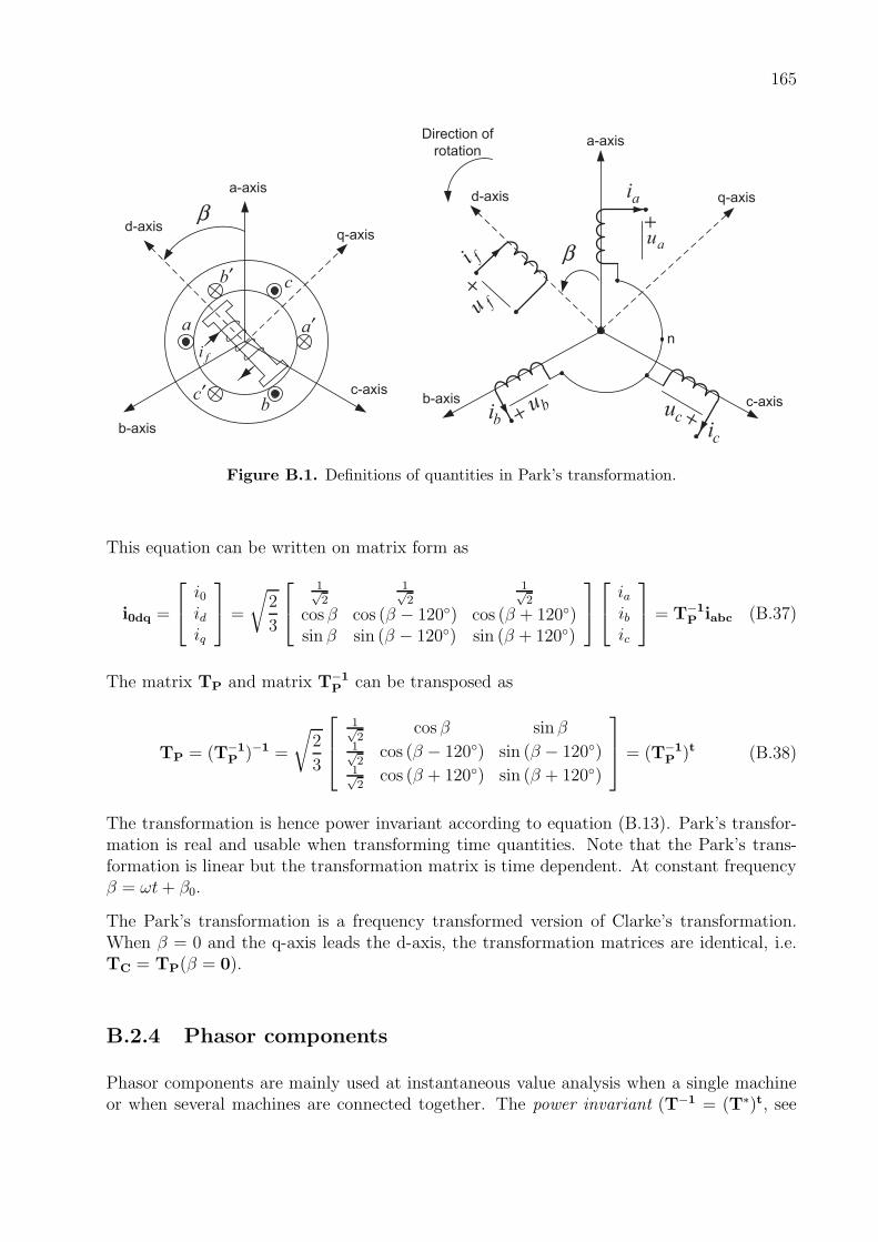
165
a-axis
b-axis
c-axis
β
a a′
b
b′ c
c′
d-axisq-axis
fi
a-axis
b-axis c-axis
β
d-axis q-axis
ci
fu+
fi
bubi
au+
ai
cu
n
++
Direction of
rotation
Figure B.1. Definitions of quantities in Park’s transformation.
This equation can be written on matrix form as
i0dq =
i0idiq
=
√
2
3
1√2
1√2
1√2
cos β cos (β − 120) cos (β + 120)sin β sin (β − 120) sin (β + 120)
iaibic
= T−1P iabc (B.37)
The matrix TP and matrix T−1P can be transposed as
TP = (T−1P )−1 =
√
2
3
1√2
cos β sin β1√2
cos (β − 120) sin (β − 120)1√2
cos (β + 120) sin (β + 120)
= (T−1
P )t (B.38)
The transformation is hence power invariant according to equation (B.13). Park’s transfor-mation is real and usable when transforming time quantities. Note that the Park’s trans-formation is linear but the transformation matrix is time dependent. At constant frequencyβ = ωt+ β0.
The Park’s transformation is a frequency transformed version of Clarke’s transformation.When β = 0 and the q-axis leads the d-axis, the transformation matrices are identical, i.e.TC = TP(β = 0).
B.2.4 Phasor components
Phasor components are mainly used at instantaneous value analysis when a single machineor when several machines are connected together. The power invariant (T−1 = (T∗)t, see

166
equation (B.13)) transformation matrix and its inverse for these components are
TR =1√3
1 ejθ e−jθ
1 α2ejθ αe−jθ
1 αejθ α2e−jθ
(B.39)
T−1R =
1√3
1 1 1e−jθ αe−jθ α2e−jθ
ejθ α2ejθ αejθ
where α = ej120
. The phasor components of the three-phase currents ia(t), ib(t) and ic(t)can be obtained as
i0(t)is(t)iz(t)
= i0sz(t) = T−1R iabc(t) =
1√3
1 1 1e−jθ αe−jθ α2e−jθ
ejθ α2ejθ αejθ
ia(t)ib(t)ic(t)
(B.40)
where i0(t) is the zero-sequence component and is(t) is called the field vector current, thecomplex phasor of the current. The current is(t) is complex since the transformation matrixis complex. By assuming that ia(t), ib(t) and ic(t) are real, the expression for iz(t) can bewritten as
iz(t) =1√3ejθ(ia(t) + α2ib(t) + αic(t)
)= (B.41)
=
[1√3e−jθ
(ia(t) + αib(t) + α2ic(t)
)]∗
= i∗s(t)
i.e. iz(t) is known if the field vector is(t) is known. Under conditions of no zero-sequencecomponents, the field vector is fully describing an arbitrary real three-phase quantity.
For a symmetrical three-phase current as given in equation (B.33), the phasor componentscan be obtained according to equation (B.40)
i0(t) =1√3(ia(t) + ib(t) + ic(t)) = 0
is(t) =e−jθ
√3
(ia(t) + αib(t) + α2ic(t)
)=
√3
2IMej(ωt−φ−θ) (B.42)
iz(t) =ejθ√3
(ia(t) + α2ib(t) + αic(t)
)=
√3
2IMe−j(ωt−φ−θ) = i
∗s(t)
Finally, for θ = ωt the following is obtained
i0(t) = 0
is(t) =
√3
2IMe−jφ (B.43)
iz(t) =
√3
2IMejφ = i
∗s(t)
i.e. the field vector current is(t) has a constant magnitude, independent of time.

167
By assuming real phase currents having no zero-sequence, they can be calculated by usingthe field vector current as
ia(t)ib(t)ic(t)
= TRi0sz(t) =1√3
1 ejθ e−jθ
1 α2ejθ αe−jθ
1 αejθ α2e−jθ
0is(t)
i∗s(t)
= (B.44)
=1√3
[ejθis(t)
]+[ejθis(t)
]∗[α2ejθis(t)
]+[α2ejθis(t)
]∗[αejθis(t)
]+[α2ejθis(t)
]∗
=2√3
Re[ejθis(t)
]
Re[α2ejθis(t)
]
Re[αejθis(t)
]
Phasor components are a frequency transformed form of the symmetrical components. Forθ = 0 (phasor components), the transformation matrix for the phasor components and thesymmetrical components are identical, i.e. TR(θ = 0) = TS.


