STATIC AND DYNAMIC MODELING OF A SOLAR ACTIVE REGION

Harry P. Warren

Space Science Division, Naval Research Laboratory, Washington, DC 20375; hwarren@nrl.navy.mil

and

Amy R. Winebarger

Department of Physics, Alabama A&M University, Normal, AL 35762; winebarger@physics.aamu.edu

Received 2006 September 1; accepted 2007 May 8

ABSTRACT

Recent hydrostatic simulations of solar active regions have shown that it is possible to reproduce both the totalintensity and the general morphology of the high-temperature emission observed at soft X-ray wavelengths usingstatic heating models. These static models, however, cannot account for the lower temperature emission. In addition,there is ample observational evidence that the solar corona is highly variable, indicating a significant role for dy-namical processes in coronal heating. Because they are computationally demanding, full hydrodynamic simulationsof solar active regions have not been considered previously. In this paper we make first application of an impulsiveheating model to the simulation of an entire active region, AR 8156 observed on 1998 February 16. We model thisregion by coupling potential field extrapolations to full solutions of the time-dependent hydrodynamic loop equa-tions. Tomake the problemmore tractable we begin with a static heatingmodel that reproduces the emission observedin four different Yohkoh Soft X-Ray Telescope (SXT) filters and consider impulsive heating scenarios that yield time-averaged SXT intensities that are consistent with the static case. We find that it is possible to reproduce the total ob-served soft X-ray emission in all of the SXT filters with a dynamical heating model, indicating that nanoflare heatingis consistent with the observational properties of the high-temperature solar corona. At EUV wavelengths the sim-ulated emission shows more coronal loops, but the agreement between the simulation and the observation is still notacceptable.

Subject headinggs: Sun: corona

1. INTRODUCTION

Understanding how the Sun’s corona is heated to high temper-atures remains one of the most significant challenges in solarphysics. Unfortunately, the complexity of the solar atmosphere,with its many disparate spatial and temporal scales, makes itimpossible to represent with a single, all-encompassing model.Instead we need to break the problem up into smaller, more man-ageable pieces (e.g., see the recent review by Klimchuk 2006).For example, kinetic theory or generalized MHD is used to de-scribe the microphysics of the energy release process. Ideal andresistive MHD are used to study the evolution of coronal mag-netic fields and the conditions that give rise to energy release.Finally, one-dimensional (1D) hydrodynamical modeling is em-ployed to calculate the response of the solar atmosphere to therelease of energy.

This last step is a critical one in the process of understandingcoronal emission, because it links theoretical models with solarobservations. Even here, however, most previous work has fo-cused on modeling small pieces of the Sun, such as individualloops (e.g., Aschwanden et al. 2001; Reale & Peres 2000). Al-though understanding the heating in individual structures isan important first step, it has been difficult to apply this infor-mation to constrain the properties of the global coronal heatingmechanism.

Recent advances in high-performance computing have madeit possible to simulate large regions of the corona, at least withstatic heating models. Schrijver et al. (2004) for example, havecoupled potential field source-surface models of the coronalmagnetic field with parametric fits to solutions of the hydrostaticloop equations to calculate visualizations of the full Sun. Com-

parisons between the simulation results and full-disk solar im-ages indicate that the energy flux (FH ) into a corona loop scalesas BF /L, where BF is the footpoint field strength, and L is theloop length. Schrijver & Title (2005) also find that this form forthe heating flux is consistent with the flux-luminosity relation-ship derived from X-ray observations of other cool dwarf stars(Schrijver & Title 2005).

Warren & Winebarger (2006) have performed similar simu-lations for 26 solar active regions using potential field extrapo-lations and full solutions to the hydrostatic loop equations. Thesesimulation results indicate that the observed emission is con-sistent with a volumetric heating rate (�S) that scales as B/L,where B is the field strength averaged along the field line. In thesample of active regions used in that study B � BF /L so thatFH � �SL � B � BF /L, and this form for the volumetric heatingrate is consistent with the energy flux determined by Schrijveret al. (2004).

In these previous studies it was possible to use static heatingmodels to reproduce the high-temperature emission observed atsoft X-ray wavelengths, but not the lower temperature emissiontypically observed in the EUV. The static models are not able toaccount for the EUV loops evident in the solar images. Recentwork has shown that the active region loops observed at theselower temperatures are often evolving (Ugarte-Urra et al. 2006;Winebarger et al. 2003). Simulation results suggest that theseloops can be understood using dynamical models, where the loopsare heated impulsively and are cooling (e.g., Spadaro et al. 2003;Warren et al. 2003). Furthermore, spectrally resolved observa-tions have indicated pervasive red shifts in active regions at up-per transition region temperatures (e.g., Winebarger et al. 2002),suggesting that much of the plasma in solar active regions near

1245

The Astrophysical Journal, 666:1245Y1255, 2007 September 10

# 2007. The American Astronomical Society. All rights reserved. Printed in U.S.A.

1 MK has been heated to higher temperatures and is cooling. Fi-nally, Warren & Winebarger (2006) found that static heating inloops with constant cross section yields footpoint emission thatis much brighter than what is observed. This suggests that staticheating models may not be consistent with the observations, evenin the central cores of active regions.

The need for exploring dynamical heating models of the solarcorona is clear, but there are a number of problems that make thisdifficult in practice. One problem is the many free parameterspossible in parameterizations of impulsive heating models. Inaddition to the magnitude and spatial location of the heating, itis possible to vary the temporal envelope and repetition rate ofthe heating (e.g., Patsourakos & Klimchuk 2006; Testa et al.2005). Furthermore, dynamical solutions to the hydrodynamicloop equations are much more computationally intensive to cal-culate than static solutions, limiting our ability to explore param-eter space.

In this paper we explore the application of impulsive heatingmodels to the high-temperature emission observed in active re-gion 8156 on 1998 February 16. To make the problem moretractable we begin with a static heatingmodel that reproduces theemission observed in four different Yohkoh Soft X-Ray Tele-scope (SXT) filters and look for dynamical models that yieldtime-averaged SXT intensities that are in agreement with thosecomputed from the static solutions. Relating the time-averagedintensities derived from the full dynamical solutions to the ob-served intensities is based on the idea that the emission from asingle feature results from the superposition of even finer, dy-namical structures that are in various stages of heating and cool-ing (Klimchuk 2006). This picture is motivated by the nanoflaremodel of coronal heating (e.g., Parker 1983; Cargill 1994;Parenti et al. 2006). Other nanoflare heating scenarios are pos-sible, such as heating events on larger scale threads that are dis-tributed randomly in space and time, but are not considered here.We find that it is possible to construct a dynamical heating modelthat reproduces the total soft X-ray emission in each SXT filter.This indicates that nanoflare heating is consistent with the ob-servational properties of the high-temperature corona. At EUVwavelengths the simulated emission shows more coronal loops,but the agreement between the simulation and the observation isstill not acceptable.

2. OBSERVATIONS

Observations from SXT (Tsuneta et al. 1991) on Yohkoh formthe basis for this work. The SXT, which operated from late 1991to late 2001, was a grazing incidence telescope with a nominalspatial resolution of about 500 (2.500 pixels). Temperature discrim-

ination was achieved through the use of several focal plane filters.The SXT response extended from approximately 3 8 to approxi-mately 40 8, and the instrument was sensitive to plasma aboveabout 2 MK.In addition to the SXT images we use full-Sun magnetograms

taken with the MDI instrument (Scherrer et al. 1995) on SOHOto provide information on the distribution of photospheric mag-netic fields. The spatial resolution of the MDI magnetograms(1.9800per pixel) is comparable to the spatial resolution of EITand SXT. In this study we use the synoptic MDI magnetograms,which are taken every 96 minutes.To constrain the static heating model we require observations

of an active region in multiple SXT filters. Observations in thethickest SXT analysis filters, the ‘‘thick aluminum’’ (Al12) andthe ‘‘beryllium’’ (Be119), are crucial for this work. As we willshow, observations in the thinner analysis filters, such as the‘‘thin aluminum’’ (Al.1) and the ‘‘sandwich’’ (AlMg) filters, donot have the requisite temperature discrimination for this mod-eling. To identify candidate observations we made a list of allSXT partial frame (as opposed to full disk) observations with ob-servations in the Al.1, AlMg, Al12, and Be119 filters betweenthe beginning of the Yohkoh mission and the end of 2001. Sincethe potential field extrapolation is also important to this analysis,we required that the active lie within 40000 of disk center.We also use consider observations from the EIT

(Delaboudiniere et al. 1995) on SOHO. EIT is a normal inci-dence telescope that takes full-Sun images in four wavelengthranges, 304 8 (which is generally dominated by emission fromHe ii), 1718 (Fe ix and Fe x), 1958 (Fe xii), and 2848 (Fe xv).EIT has a spatial resolution of 2.600. Images in all four wave-lengths are typically taken four times a day, and these synopticdata are used in this study.From a visual inspection of the available data we selected ob-

servations ofAR8156 taken 1998February 16 near 8UT. This re-gion is shown in full-disk SXTandMDI images in Figure 1. Theregion of interest observed in SXT, EIT, and MDI is shown in Fig-ure 2. These images represent the observations taken closest to theMDImagnetogram. The total intensities in the SXT partial frameimages for this region during the period beginning 1998 Feb-ruary 15 23:30 UT and ending 1998 February 16 13:00 UT aregenerally within �20% of the total intensities in these SXT im-ages, indicating an absence ofmajor flare activity during this time.

3. STATIC MODELING

To model the topology of this active region we use a simplepotential field extrapolation of the photospheric magnetic field.For each MDI pixel with a field strength greater than 50 G we

Fig. 1.—Observations of AR 8156 on 1996 February 16 near 08:00 UT in SXT (center) andMDI (right). The field of view of the SXT partial frame images is indicatedby the box.

WARREN & WINEBARGER1246 Vol. 666

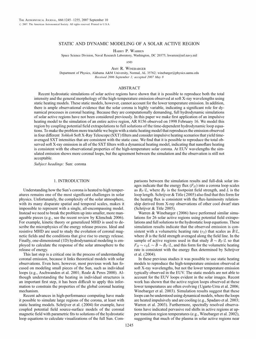
calculate a field line. Some representative field lines are shown inFigure 2. It is clear that such a simple model does not fully re-produce the observed topology of the images. The long loops inthe bottom half of the images, for example, are shifted relative tothe field lines computed from the potential field extrapolation.However, as we argued previously (Warren &Winebarger 2006),our goal is not to reproduce the exact morphology of the activeregion. Rather, we are primarily interested in the more generalproperties of the active region emission, such as the total intensityor the distribution of intensities. The potential field extrapolationonly serves to provide a realistic distribution of loop lengths.

One subtlety with coupling a potential field extrapolation withsolutions to the hydrostatic loop equations is the difference inboundary conditions. The field lines originate in the photosphere,where the plasma temperature is approximately 4000 K. Theboundary condition for the loop footpoints, however, are typi-cally set at 10,000 or 20,000 K in the numerical solutions to thehydrodynamic loop equations. Furthermore, studies of the topol-ogy of the quiet Sun have shown that a significant fraction of thefield lines close at heights below 2.5 Mm, a typical chromo-spheric height (Close et al. 2003). To avoid these small scaleloops we use the portion of the field line above 2.5 Mm in themodeling and exclude all field lines that do not reach this height.

For each of the 1956 field lines ultimately included in the sim-ulation we calculate a solution to the hydrostatic loop equations

using a numerical code written by Aad van Ballegooijen (e.g.,Hussain et al. 2002; Schrijver & van Ballegooijen 2005). Fol-lowing our previous work, our volumetric heating function isassumed to be

�S ¼ �0 B=B0

� �L0=Lð Þ; ð1Þ

where B is the field strength averaged along the field line, and L isthe total loop length. The values adopted for the parameters B0

and L0 are 76 G and 29 Mm, respectively. We assume a constantcross section and a uniform distribution of heating along eachloop. Note that the variation in gravity along the loop is deter-mined from the geometry of the field line.

The numerical solution to the hydrostatic loop equation pro-vides the variation in the density, temperature, and velocity alongthe loop. The temperatures, densities, and loop geometry are thenused to compute the expected response in the SXT and EIT fil-ters. For our work we use the CHIANTI atomic database (e.g.,Dere et al. 1997) to compute the instrumental responses and theradiative losses used in the hydrostatic code (see Brooks &Warren 2006 for a discussion of the instrumental responses andradiative losses).

In our previous work the value for �0 was chosen to be0.0492 erg cm�3 s�1 so that a ‘‘typical’’ field line (B ¼ B0 and

Fig. 2.—Top panels: Selected field lines from the potential field extrapolation of the MDI magnetogram taken at 08:00:03 UT.Middle panels: EIT synoptic images ofAR 8156 in all four EIT wavelengths. Bottom panels: SXT images in four filters.

ACTIVE REGION MODELING 1247No. 2, 2007

L ¼ L0) had an apex temperature of T0 ¼ 4MK. We also foundthat for this value of �0 a filling factor of about 10% was neededto reproduce the SXT emission observed in the Al.1 or AlMg fil-ters. In the absence of information from the hotter SXT filters thevalue for �0 is poorly constrained.

For this active region we have observations in the hotter SXTfilters, so we have performed active region simulations for arange of T0 (equivalently �0) values. The resulting total inten-sities in each of the four filters as a function of T0 are shown inFigure 3. It is clear from this figure that the static model cannotreproduce all of the SXT intensities for a filling factor of 1. Fora filling factor of 1 the value of T0 needed to reproduce theAl.1 intensity yields a Be119 intensity that is too low. Similarly,the value of T0 that reproduces the Be119 intensity for a fillingfactor of 1 yields Al.1 intensities that are too large.

By doing a least-squares fit of the simulation results to theobservations and varying both the value of T0 and the fillingfactor we find that we can reproduce all of the SXT intensities towithin 10% for T0 ¼ 3:8MK and a filling factor of 7.6%, valuesclose to what we used in our previous work. These simulationresults also highlight the importance of the SXTAl12 and Be119filters in modeling the observations. The ratio between the Al.1and AlMg filters is simply too shallow to be of any use in con-straining the magnitude of the heating. The Al.1 to Be119 ratio,in contrast, varies by almost an order of magnitude as T0 is variedfrom 2 to 5 MK.

The total intensity represents the minimum level of agreementbetween the simulation and the observations. The distribution ofthe simulated intensities must also look similar to what is ob-served. To transform the 1D intensities into 3D intensities we as-sume that the intensity at any point in space is related to theintensity on the field line by

I(x; y; z) ¼ k I(x0; y0; z0) exp � �2

2�2r

� �; ð2Þ

where �2 ¼ (x� x0)2 þ ( y� y0)

2 þ (z� z0)2 and 2:355�r, the

FWHM, is set equal to the assumed diameter of the flux tube. Asin our previous work we use the width of a full-disk MDI pixel(1.9800) for the diameter. A normalization constant (k) is introducedso that the integrated intensity of over all space is equal to the inten-sity integrated along the field line. This approach for the visualiza-tion is based on the method used in Karpen et al. (2001). The SXTimages are convolved with the instrumental point-spread function.One change that we have made from our previous method-

ology (Warren & Winebarger 2006) is to include all of the fieldlines with footpoint field strengths above 500G. These field lineshave been largely excluded in previous work, because sunspotsare generally faint in soft X-rays images (see Golub & Pasachoff1997; Schrijver et al. 2004; Fludra& Ireland 2003). In these obser-vations, however, the exclusion of the field lines rooted in strongfield leads to small, but noticeable differences between the sim-ulated and observed emission. As can be inferred from Figure 2,excluding these field lines leads to an absence of emission oneither side of the bright feature in the center of the active region.This suggests that the algorithm used to select which field linesare included in the simulation needs to be studied more carefully.The resulting simulated SXT images are shown in Figure 4

where they are compared with the observations. The simulationsclearly do a reasonable job reproducing these data, particularly inthe core of the active region. At the periphery of the active regionthe simulation does not match either themorphology of the emis-sion or its absolute magnitude exactly. The general impression,however, is that the model intensities are generally similar to theobserved intensities outside of the active region core even if themorphology is somewhat different.The histograms of the intensities offer an additional point of

comparison between the simulations and the observations. Asshown in Figure 4, the distributions of the intensities are verysimilar in both cases, supporting the qualitative agreement be-tween the visualizations and the actual solar images.

Fig. 3.—Simulated and observed SXT intensities for AR 8156. Top left panel: The simulated intensities as a function of T0 assuming a filling factor of unity. Theobserved intensities in each filter are indicated with the dotted lines. Simulations are calculated in steps of 0.5 MK. Other panels: Simulated filter ratios, which areindependent of the filling factor, as a function of T0. The observed filter ratios are indicated by the dotted lines. The best-fit value for T0 is also indicated on these plots.

WARREN & WINEBARGER1248 Vol. 666

The good agreement between the simulation and the observa-tions seen in the soft X-ray images does not extend to the coolerEUV emission. In Figure 5 we see that the simulated EIT 171,195, and 2848 emission is dominated by the moss emission (thetransition region of high-temperature loops, Berger et al. 1999),and there is no looplike emission in the simulation. We also seethat the simulated moss emission is much brighter than what isobserved. These simulation results indicate that static heatingcannot fully account for the observed emission in an active re-gion. Given the success of impulsive heating models in repro-ducing some aspects of the emission observed in the EUV, at

least qualitatively, it is natural to wonder how we might modelthe SXT emission with time-dependent heating.

4. DYNAMIC MODELING

The principal difficulties with full hydrodynamic modelingof solar active regions are the many degrees of freedom avail-able to parameterize the heating function and the computationaldifficulty of calculating the numerical solutions. For this explor-atory study we make several simplifying assumptions. First, weconsider dynamic simulations that are closely related to the staticsolutions. Since the static modeling of the SXT observations

Fig. 4.—Observed and simulated SXT emission for AR 8156. These results are from the static heating model. Top panels: Observed and simulated images. Thecalculated SXT images have been convolved with the SXT point-spread function. The numbers in parentheses indicate the total intensity in the image. Bottom panels: Theintensity distributions for the observed and simulated images.

ACTIVE REGION MODELING 1249No. 2, 2007

Fig. 5.—Observed and simulated EIT emission for AR 8156. These results are from the static heating model. In the static heating simulation the EUV emission isdominated by the moss. Since the morphology of the simulated images does not match the observations, the comparisons of the total intensities are not meaningful and thetotal intensities are not indicated. Also note that the EIT images have not been convolved with the instrumental point-spread function.

Fig. 6.—Comparison of static and dynamic simulations of SXT emission. The parameters for the static case are L ¼ 66 Mm and �S ¼ 0:091 erg cm�3 s�1, and aretypical of the active region simulation. For the dynamic case R ¼ 1:8, and the heating duration is 200 s. Left panels: The evolution of the temperatures and densitiesaveraged over the top 10%of the loop apex.Right panels: The evolution of the intensities in four SXTfilters. The SXT intensities from the staticmodel, including the fillingfactor from the active region simulation, are also shown. For this case the SXT intensities from the time-averaged dynamic simulation are very close to those from the staticsimulation.

presented in x 3 adequately reproduces the total intensities, thedistribution of intensities, and the general morphology of theimages, it seems reasonable to consider dynamical heating thatwould reproduce the static solutions in some limit. Second, weutilize the time-averaged properties of these solutions in com-puting the simulated intensities. Our assumption is that the emis-sion from a single field line in the static model actually resultsfrom the superposition of even finer, dynamical structures thatare in various stages of heating and cooling. This assumption ismotivated by the nanoflare model of coronal heating (e.g., Parker1983; Cargill 1994; Parenti et al. 2006).

In the static case we have used the average magnetic fieldstrength and loop length to infer the volumetric heating rate (�s)for each field line. For the dynamic case we consider volumetricheating rates of the form

�D(t) ¼ g (t)R�S þ �B; ð3Þ

where g (t) is a step or boxcar function envelope on the heating,�S is the static heating rate determined from equation (1), R is aarbitrary scaling factor, and �B is a weak background heating ratethat establishes a cool, tenuous equilibrium atmosphere in theloop. To solve the hydrodynamic loop equations numerically weuse the NRL Solar Flux Tube Model (SOLFTM) code (e.g.,Mariska 1987; Mariska et al. 1989).

In the limit of an infinite heating window and R ¼ 1 the dy-namic solutions would converge to the static solutions, and all ofthe properties of the static simulation would be recovered. Thisis the primary motivation for our choice of the heating functiongiven in equation (3). The good agreement between the obser-vations and the static model suggest that the energetics of thestatic model are not far off.

For R ¼ 1 and a finite duration to the heating, we expect thatthe calculated SXT emission will generally be less than in thestatic case, because it takes a finite time for chromospheric plasmato evaporate up into the loop. Thus, simply truncating the heatingwill not produce acceptable results. If we increase the heatingsomewhat from the static case (R > 1) and consider a finite du-ration, we expect larger SXT intensities relative to the R ¼ 1,finite-duration case, since the evaporation will be faster and thetemperatures will be higher with the increased heating. Since thetime to fill the loop with plasma will depend on the sound cross-ing time (�s � L/cs, with cs the sound speed), the behavior of thedynamic solutions relative to the static solutions will also dependon loop length. For a finite duration to the heating the intensitiesin the dynamical simulations of the shorter loops will moreclosely resemble the results from the static solution.

An illustrative dynamical simulation is shown in Figure 6.Here R ¼ 1:8 and the heating duration is 200 s. For these pa-rameters the apex densities are somewhat lower than the corre-sponding static solution. The time averaging also reduces theSXT intensities significantly relative to their peak values. Whenthe filling factor is included in the calculation of the SXT inten-sities from the static solutions, however, we see that the SXTintensities calculated from the two different simulations are verysimilar in all of the filters of interest.

Note that the computed intensities are somewhat dependenton the interval chosen for the time averaging. We assume thateach small-scale thread is heated once then allowed to cool fullybefore being heated again. In practice, we terminate the dynam-ical simulation when the apex temperature falls below 0.7 MK.The SOLFTM code only has an adaptive mesh in the transitionregion and cannot resolve the formation of very cool materialin the corona. Radiative losses become very large at low temper-

atures, so the loops evolve very rapidly past this point and thetime-averaged intensities should be only weakly dependent onwhen the dynamical simulation is stopped.

While calculations such as this, which show that the SXTintensities computed from the dynamical simulation and thosecomputed from the static simulation can be comparable, areencouraging, they represent a special case. In general, for a fixedvalue of R the ratio of the dynamic and static intensities will begreater than 1 for shorter loops and smaller than 1 for longer loops.We would like to know what would happen if we performed dy-namical simulations for all of the loops in AR 8156.

To apply the impulsive heating model to the active region foreach field line, we must find the value of R that makes the time-averaged intensities equal to the static intensities, such as is il-lustrated in Figure 6. To accomplish this we use a brute forceapproach and consider grids of solutions that encompass therange of loop lengths and heating rates that are present in ourstatic simulation of this active region.

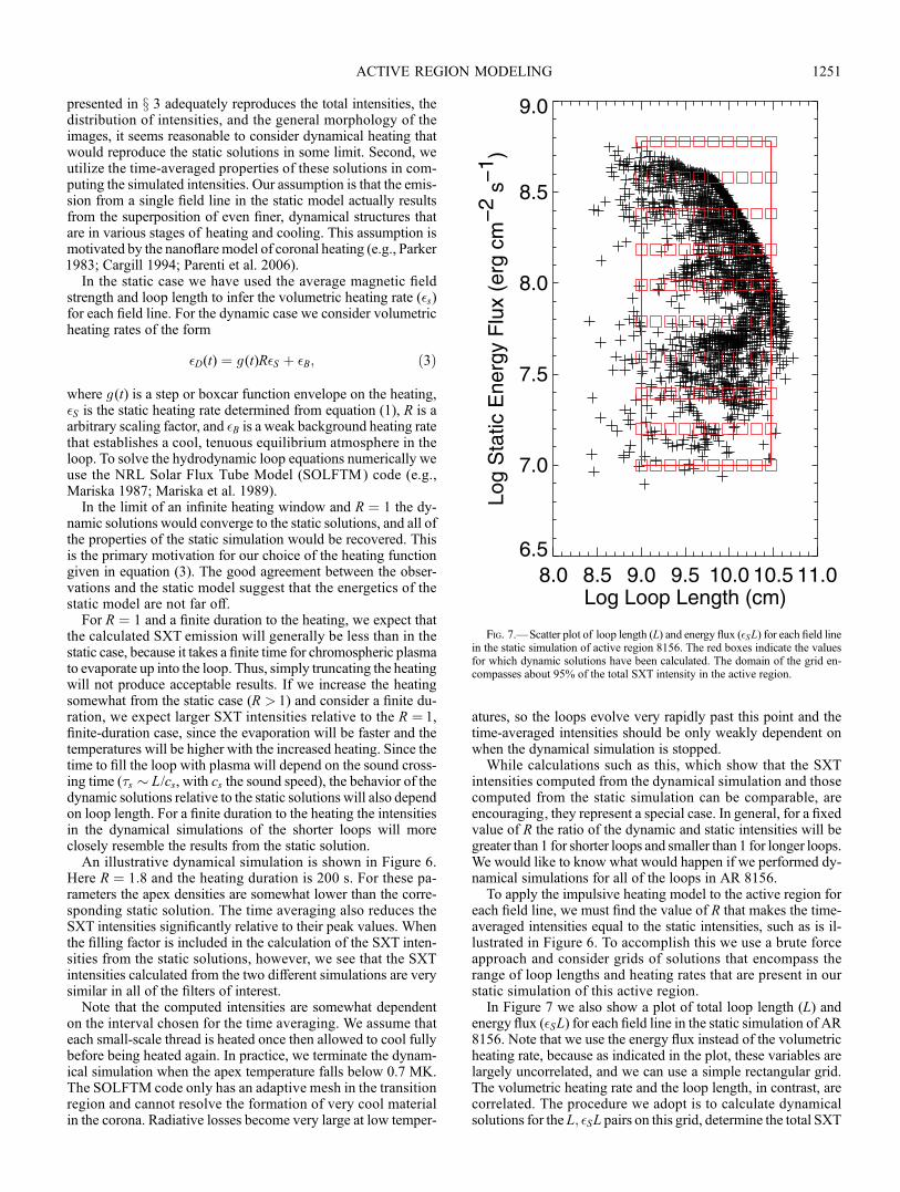
In Figure 7 we also show a plot of total loop length (L) andenergy flux (�SL) for each field line in the static simulation of AR8156. Note that we use the energy flux instead of the volumetricheating rate, because as indicated in the plot, these variables arelargely uncorrelated, and we can use a simple rectangular grid.The volumetric heating rate and the loop length, in contrast, arecorrelated. The procedure we adopt is to calculate dynamicalsolutions for the L; �SL pairs on this grid, determine the total SXT

Fig. 7.—Scatter plot of loop length (L) and energy flux (�SL) for each field linein the static simulation of active region 8156. The red boxes indicate the valuesfor which dynamic solutions have been calculated. The domain of the grid en-compasses about 95% of the total SXT intensity in the active region.

ACTIVE REGION MODELING 1251

intensities for these solutions, and then use interpolation to es-timate the SXT intensities for each field line in the simulation. Toinvestigate the effects of varying R on the dynamical solutionswe have computed seven 10 ; 10 grids for log R ¼ ½�0:5; 1� fora total of 700 dynamical simulations. These calculations whereperformed on a 100 node parallel computer.

One important difference between these grid solutions and thestatic solutions discussed in x 3 is the loop geometry. In the staticsimulation the loop geometry is determined by the field line.In the dynamic simulation the loop is assumed to be perpendic-ular to the solar surface. Since the density scale height for high-temperature loops is large, this difference has only a small effecton the simulation of the SXT emission.

In Figure 8 we summarize the resulting SXTAl12 intensitiesfor the seven solution grids. In these plots we show the ratio ofthe time-averaged intensity from the impulsive heating model tothe intensity computed from the static model. That is, we com-pare the total intensity determined from the static solution witha heating rate of �S with the total intensity determined with thetime-dependent heating rate �D given in equation (3).As expected,the most intense loops in the dynamic simulations are the shortestloops with the most intense heating. The faintest loops are thelongest loops with the weakest heating.

We have used the results from the computational grids to cal-culate the value of R needed to produce time-averaged intensi-ties that are equal to the static intensities as a function of theloop length and the energy flux. We refer to this special value ofR as R�. An example calculation is shown in Figure 9. All of thevalues for R� for this computational grid are summarized in Fig-ure 8. The values forR� depend onlymarginally on the SXT filterselected for this analysis.

The result of this rather lengthy computational exercise is theability to reproduce the observed SXT emission with the im-pulsive heating model described in equation (3). To confirm thiswe determine the appropriate value of R� for each of the nearly2000 field line in the static simulation by interpolating on the gridshown in Figure 8. We then run the hydrodynamic simulationand calculate the SXT intensities for each computational cell

along the loop at a 30 s cadence [Ik(s; t)]. We then map the time-averaged intensities [hIk(s; t)i] onto the field line and produce asynthetic image. Note that there is a mismatch between the actualgeometry of the field line and the perpendicular geometry as-sumed in the hydrodynamic simulation. As we argued earlier, thescale height at these temperatures is generally comparable to orlonger than the loop length, so that this should be a relativelysmall effect.The SXTemission calculated from the impulsive heating sim-

ulation is shown in Figure 10. The morphology of these simu-lated images is nearly identical to that determined from the static

Fig. 8.—Left panels: The ratio of dynamic to static SXT intensity as a function of R. The solid contour indicates where the static and dynamic intensities are equal.Right-most panel: The value of R� as a function of loop length and energy flux as determined from the grids.

Fig. 9.—Illustration of the use of the computational grids to find R� for agiven loop length and static heating rate.

WARREN & WINEBARGER1252

Fig. 10.—Observed and simulated emission for AR 8156. These simulation results are from the impulsive heating model. SXT images (top panels), EIT images(middle panels). Because of the complexity of the formation process simulated 3048 images have not been calculated. The simulated EITemission seen edge-on (bottompanels). The vertical extent of the image is 15500.

heating model. The relative intensities in the different SXT fil-ters, however, are slightly different. The duration of the heating islikely to be closely related to the peak temperatures observed inthe loops. It is possible that a slightly shorter duration would leadto better agreement, but this has not yet been investigated.

One of the primary motivations for considering the impulsiveheating model is the possibility of better reproducing the emis-sion observed at lower temperatures. For this reason we havealso calculated the EIT emission from the hydrodynamic simu-lation and produced the synthetic images shown in Figure 10.Wenote that as with the SXT emission, the time-averaged intensi-ties are mapped onto field lines. The pressure scale heights atthese lower temperatures are smaller, however, leading to largerdiscrepancies between the geometry of the field line and theperpendicular orientation used in the calculation. Thus thesecalculations should be regarded with some caution.

The simulated EIT images indicate that the dynamic heat-ing model does produce more loop emission in the corona. Thisis particularly evident when the emission is viewed edge-on(Fig. 10, bottom panels). In the staticmodels this view shows onlya thin layer of emission. In the dynamic simulation bright loopemission extends well into the corona. Despite the presence ofmore loop emission, the agreement between the simulation andthe observation is still not acceptable. In the simulation the loopemission is a dominant feature of the core of the active region,while in the observations the loops are found primarily outsidethe core of the active region. In addition, the EUV intensities inthe core of the active region are too bright relative to what is ob-served. While these simulations represent an advance over ourprevious modeling efforts, a comprehensive understanding of ac-tive region heating, even at a phenomenological level, remainselusive.

5. SUMMARY AND DISCUSSION

We have investigated the use of static and dynamic heatingmodels in the simulation of AR 8156. Recent work has shownthat static models can capture many of the observed properties ofthe high-temperature soft X-ray emission from solar active re-gions, and our results confirm this. We are able to reproduce boththe total intensity and the general morphology of this active re-gion with a static heating model. Furthermore, our results showthat this agreement extends to the hotter SXT filters, which havenot been considered before.

The application of dynamic heating models to active regionemission on this scale has not been considered previously. Mostpast work has focused on the properties of individual loops (e.g.,Reale et al. 2000; Warren et al. 2002). In this paper we haveinvestigated an impulsive heating model that is motivated by thestatic simulations. We have shown that it is possible to reproducethe SXT emission using hydrodynamic simulations. The impul-sive heating model also produces significant loop emission at thelower temperatures imaged in the EITchannels. Themorphologyof the simulated EUVemission, however, does not agree with theobservations.

Conceptually, the simple dynamical heatingmodel investigatedhere, where we assume that the emission from a solar feature re-sults from the superposition of many, very fine structures that arein various stages of heating and cooling, is closely related to thenanoflare model of coronal heating (e.g., Parker 1983; Cargill1994). The use of time-averaged intensities computed from thedynamical simulations implicitly assumes that the heating is verycoherent, with each infinitesimal thread being heated once andthen allowed to cool and drain before being heated again.

The inability of this heating model to adequately reproducethe observed EUV emission indicates that we must consider al-ternative scenarios. One possibility is that the heating in the co-rona is occurring on larger scale threads that are energized morefrequently. The analysis of high spatial resolution (0.500) EUVimages suggests that current solar instrumentation may be closeto resolving individual threads in the corona (Aschwanden 2005;Aschwanden & Nightingale 2005). Considerable work remainsto be done to determine the fundamental spatial scale for coronalheating. Intermittent heating, particularly in the core of the activeregion, would keep the loops at high temperatures and preventthe formation of cool EUV loops. Extended gaps in the heating,however, would allow for catastrophic cooling (e.g., Schrijver2001) and the intermittent formation of EUV loops. The impli-cations of an intermediate timescale for the heating has not yetbeen fully investigated.The geometrical properties of coronal threads is also unclear

at present. We have assumed constant cross sections in our mod-eling, consistent with the observational results (Klimchuk et al.1992; Watko & Klimchuk 2000). In the static modeling ofsolar active regions there has been some evidence that the loopswith expanding cross sections better reproduce the observations(Schrijver et al. 2004; Warren & Winebarger 2006). Detailedcomparisons between simulated and observed solar images areneeded to resolve this issue.In comparing the observed and simulated emission at the

lower temperatures is also important to consider several compli-cations. The ambient solar corona is at a temperature of about1.5 MK (e.g., Warren & Warshall 2002), which means that therelatively cool active region loops imaged with EIT are embed-ded in a plasma that is emitting strongly at the samewavelengths.This leads to a relatively low contrast between the corona and theloops (Cirtain et al. 2006) and implies that the backgroundcorona makes a significant contribution to the total emission inan image (e.g., Brooks & Warren 2007). Separately, the mossintensities, which are a potentially powerful diagnostic of thecoronal heating (e.g., Martens et al. 2000), are also influenced byspicular absorption (Berger et al. 1999). Thus, simulated inten-sities that appear to be excessively bright may in fact be con-sistent with the observations once absorption is included.Despite the many limitations to our modeling, the results that

we have presented are encouraging and provide a framework forfurther exploration. The highest priority for future work is theconsideration of models with intermittent heating. Anotherpriority is the comparison of active region simulations withspatially and spectrally resolved observations from the recentlylaunchedHinode (formally Solar-B)mission. Spectral diagnostics,such as Doppler velocities, nonthermal widths, and plasma den-sities, are another dimension that have not been explored in thecontext of this modeling.

The authors would like to thank John Mariska for his helpfulcomments on the manuscript. The authors are also grateful to thereferee for encouraging us to pursuemore ambitious simulations.The hydrodynamic calculations presented here were performedon the Naval Research Laboratory Space Science Division super-computing cluster. Yohkoh is a mission of the Institute of Spaceand Astronautical Sciences (Japan), with participation from theU.S. and U.K. The EIT data are courtesy of the EIT consortium.This research was supported by NASA’s Supporting Researchand Technology and Guest Investigator programs and by the Of-fice of Naval Research.

WARREN & WINEBARGER1254 Vol. 666

REFERENCES

Aschwanden, M. J. 2005, ApJ, 634, L193Aschwanden, M. J., & Nightingale, R. W. 2005, ApJ, 633, 499Aschwanden, M. J., Schrijver, C. J., & Alexander, D. 2001, ApJ, 550, 1036Berger, T. E., de Pontieu, B., Schrijver, C. J., & Title, A. M. 1999, ApJ, 519,L97

Brooks, D. H., & Warren, H. P. 2006, ApJS, 164, 202———. 2007, ApJ, submittedCargill, P. J. 1994, ApJ, 422, 381Cirtain, J., Martens, P. C. H., Acton, L. W., & Weber, M. 2006, Sol. Phys., 235,295

Close, R. M., Parnell, C. E., Mackay, D. H., & Priest, E. R. 2003, Sol. Phys.,212, 251

Delaboudiniere, J.-P., et al. 1995, Sol. Phys., 162, 291Dere, K. P., Landi, E., Mason, H. E., Monsignori Fossi, B. C., & Young, P. R.1997, A&AS, 125, 149

Fludra, A., & Ireland, J. 2003, in The Future of Cool-Star Astrophysics: 12thCambridge Workshop on Cool Stars, Stellar Systems, and the Sun, ed. A.Brown, G. M. Harper, & T. R. Ayres (Boulder: Univ. Colorado Press), 220

Golub, L., & Pasachoff, J. M. 1997, The Solar Corona (Cambridge: CambridgeUniv. Press)

Hussain, G. A. J., van Ballegooijen, A. A., Jardine, M., & Collier Cameron, A.2002, ApJ, 575, 1078

Karpen, J. T., Antiochos, S. K., Hohensee, M., Klimchuk, J. A., & MacNeice,P. J. 2001, ApJ, 553, L85

Klimchuk, J. A. 2006, Sol. Phys., 234, 41Klimchuk, J. A., Lemen, J. R., Feldman, U., Tsuneta, S., & Uchida, Y. 1992,PASJ, 44, L181

Mariska, J. T. 1987, ApJ, 319, 465

Mariska, J. T., Emslie, A. G., & Li, P. 1989, ApJ, 341, 1067Martens, P. C. H., Kankelborg, C. C., & Berger, T. E. 2000, ApJ, 537, 471Parenti, S., Buchlin, E., Cargill, P. J., Galtier, S., & Vial, J.-C. 2006, ApJ, 651,1219

Parker, E. N. 1983, ApJ, 264, 642Patsourakos, S., & Klimchuk, J. A. 2006, ApJ, 647, 1452Reale, F., & Peres, G. 2000, ApJ, 528, L45Reale, F., Peres, G., Serio, S., Betta, R. M., DeLuca, E. E., & Golub, L. 2000,ApJ, 535, 423

Scherrer, P. H., et al. 1995, Sol. Phys., 162, 129Schrijver, C. J. 2001, Sol. Phys., 198, 325Schrijver, C. J., Sandman, A. W., Aschwanden, M. J., & DeRosa, M. L. 2004,ApJ, 615, 512

Schrijver, C. J., & Title, A. M. 2005, ApJ, 619, 1077Schrijver, C. J., & van Ballegooijen, A. A. 2005, ApJ, 630, 552Spadaro, D., Lanza, A. F., Lanzafame, A. C., Karpen, J. T., Antiochos, S. K.,Klimchuk, J. A., & MacNeice, P. J. 2003, ApJ, 582, 486

Testa, P., Peres, G., & Reale, F. 2005, ApJ, 622, 695Tsuneta, S., et al. 1991, Sol. Phys., 136, 37Ugarte-Urra, I., Winebarger, A. R., & Warren, H. P. 2006, ApJ, 643, 1245Warren, H. P., & Warshall, A. D. 2002, ApJ, 571, 999Warren, H. P., & Winebarger, A. R. 2006, ApJ, 645, 711Warren, H. P., Winebarger, A. R., & Hamilton, P. S. 2002, ApJ, 579, L41Warren, H. P., Winebarger, A. R., & Mariska, J. T. 2003, ApJ, 593, 1174Watko, J. A., & Klimchuk, J. A. 2000, Sol. Phys., 193, 77Winebarger, A. R., Warren, H. P., & Seaton, D. B. 2003, ApJ, 593, 1164Winebarger, A. R., Warren, H., van Ballegooijen, A., DeLuca, E. E., & Golub,L. 2002, ApJ, 567, L89

ACTIVE REGION MODELING 1255No. 2, 2007