Statically Determinate Plane Frames 4 Abstract Plane frame structures are composed of structural members which lie in a single plane. When loaded in this plane, they are subjected to both bending and axial action. Of particular interest are the shear and moment distributions for the members due to gravity and lateral loadings. We describe in this chapter analysis strategies for typical statically determi- nate single-story frames. Numerous examples illustrating the response are presented to provide the reader with insight as to the behavior of these structural types. We also describe how the Method of Virtual Forces can be applied to compute displacements of frames. The theory for frame structures is based on the theory of beams presented in Chap. 3. Later in Chaps. 9, 10, and 15, we extend the discussion to deal with statically indeterminate frames and space frames. 4.1 Definition of Plane Frames The two dominant planar structural systems are plane trusses and plane frames. Plane trusses were discussed in detail in Chap. 2. Both structural systems are formed by connecting structural members at their ends such that they are in a single plane. The systems differ in the way the individual members are connected and loaded. Loads are applied at nodes (joints) for truss structures. Consequently, the member forces are purely axial. Frame structures behave in a completely different way. The loading is applied directly to the members, resulting in internal shear and moment as well as axial force in the members. Depending on the geometric configuration, a set of members may experience predomi- nately bending action; these members are called “beams.” Another set may experience predominately axial action. They are called “columns.” The typical building frame is composed of a combination of beams and columns. Frames are categorized partly by their geometry and partly by the nature of the member/member connection, i.e., pinned vs. rigid connection. Figure 4.1 illustrates some typical rigid plane frames used mainly for light manufacturing factories, warehouses, and office buildings. We generate three- dimensional frames by suitably combining plane frames. # Springer International Publishing Switzerland 2016 J.J. Connor, S. Faraji, Fundamentals of Structural Engineering, DOI 10.1007/978-3-319-24331-3_4 305
Transcript
Statically Determinate Plane Frames 4
Abstract
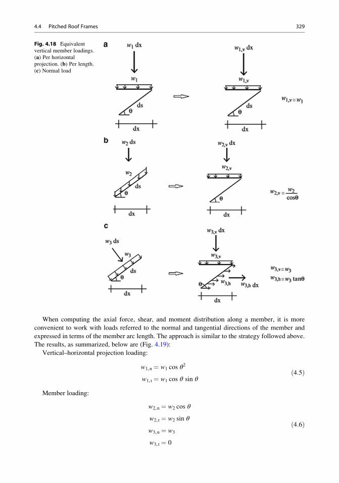
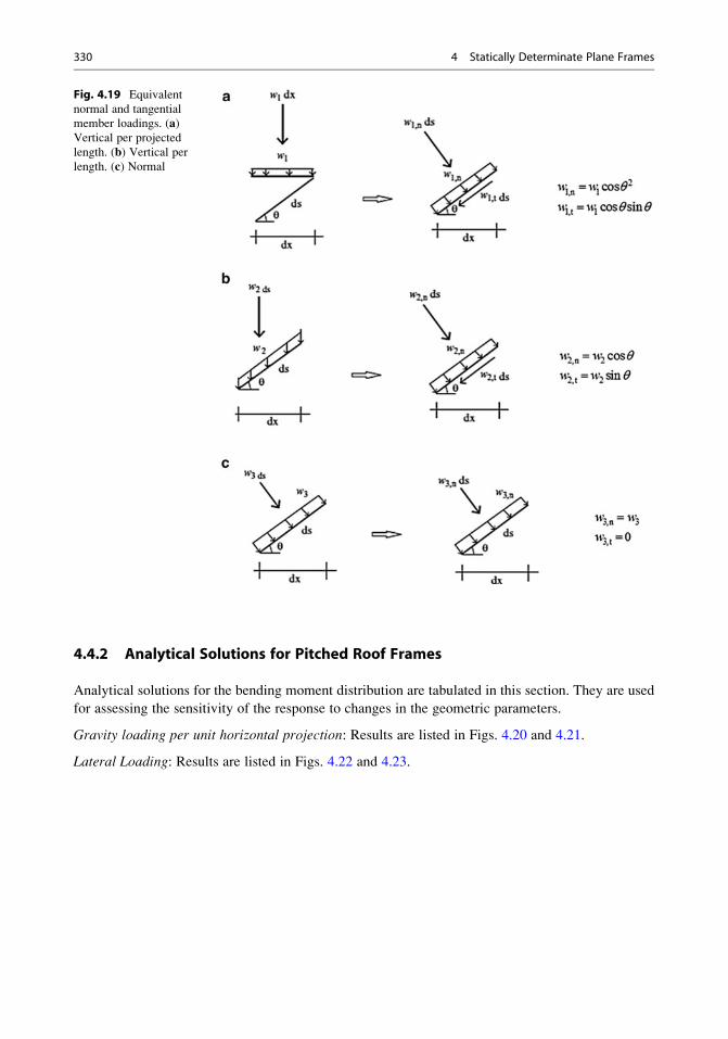
Plane frame structures are composed of structural members which lie in a
single plane. When loaded in this plane, they are subjected to both
bending and axial action. Of particular interest are the shear and moment
distributions for the members due to gravity and lateral loadings. We
describe in this chapter analysis strategies for typical statically determi-
nate single-story frames. Numerous examples illustrating the response are
presented to provide the reader with insight as to the behavior of these
structural types. We also describe how the Method of Virtual Forces can
be applied to compute displacements of frames. The theory for frame
structures is based on the theory of beams presented in Chap. 3. Later in
Chaps. 9, 10, and 15, we extend the discussion to deal with statically
indeterminate frames and space frames.
4.1 Definition of Plane Frames
The two dominant planar structural systems are plane trusses and plane frames. Plane trusses were
discussed in detail in Chap. 2. Both structural systems are formed by connecting structural members
at their ends such that they are in a single plane. The systems differ in the way the individual members
are connected and loaded. Loads are applied at nodes (joints) for truss structures. Consequently, the
member forces are purely axial. Frame structures behave in a completely different way. The loading
is applied directly to the members, resulting in internal shear and moment as well as axial force in the
members. Depending on the geometric configuration, a set of members may experience predomi-
nately bending action; these members are called “beams.” Another set may experience predominately
axial action. They are called “columns.” The typical building frame is composed of a combination of
beams and columns.
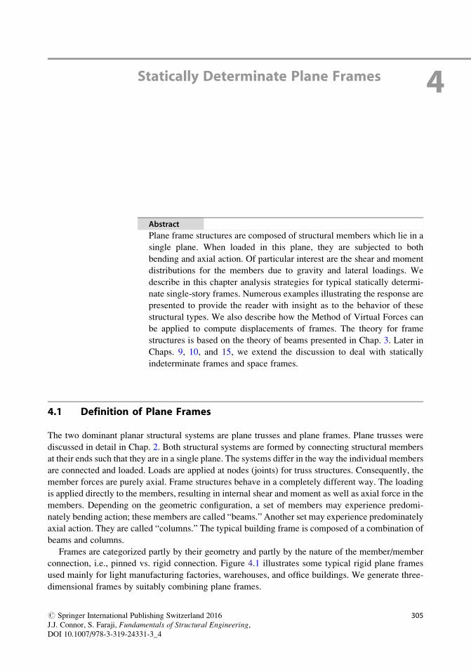
Frames are categorized partly by their geometry and partly by the nature of the member/member
connection, i.e., pinned vs. rigid connection. Figure 4.1 illustrates some typical rigid plane frames
used mainly for light manufacturing factories, warehouses, and office buildings. We generate three-
dimensional frames by suitably combining plane frames.
# Springer International Publishing Switzerland 2016
J.J. Connor, S. Faraji, Fundamentals of Structural Engineering,DOI 10.1007/978-3-319-24331-3_4
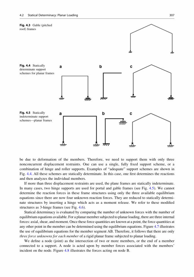
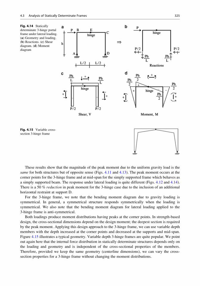
be due to deformation of the members. Therefore, we need to support them with only three
nonconcurrent displacement restraints. One can use a single, fully fixed support scheme, or a
combination of hinge and roller supports. Examples of “adequate” support schemes are shown in
Fig. 4.4. All these schemes are statically determinate. In this case, one first determines the reactions
and then analyzes the individual members.
If more than three displacement restraints are used, the plane frames are statically indeterminate.
In many cases, two hinge supports are used for portal and gable frames (see Fig. 4.5). We cannot
determine the reaction forces in these frame structures using only the three available equilibrium
equations since there are now four unknown reaction forces. They are reduced to statically determi-
nate structures by inserting a hinge which acts as a moment release. We refer to these modified
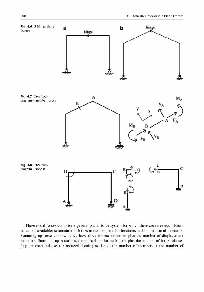
structures as 3-hinge frames (see Fig. 4.6).
Statical determinacy is evaluated by comparing the number of unknown forces with the number of
equilibrium equations available. For a planarmember subjected to planar loading, there are three internal
forces: axial, shear, andmoment. Once these force quantities are known at a point, the force quantities at
any other point in the member can be determined using the equilibrium equations. Figure 4.7 illustrates
the use of equilibrium equations for the member segment AB. Therefore, it follows that there are only
three force unknowns for each member of a rigid planar frame subjected to planar loading.
We define a node (joint) as the intersection of two or more members, or the end of a member
connected to a support. A node is acted upon by member forces associated with the members’
incident on the node. Figure 4.8 illustrates the forces acting on node B.
Fig. 4.3 Gable (pitched
roof) frames
Fig. 4.4 Statically
determinate support
schemes for planar frames
Fig. 4.5 Statically
indeterminate support
schemes—planar frames
4.2 Statical Determinacy: Planar Loading 307
These nodal forces comprise a general planar force system for which there are three equilibrium
equations available; summation of forces in two nonparallel directions and summation of moments.
Summing up force unknowns, we have three for each member plus the number of displacement
restraints. Summing up equations, there are three for each node plus the number of force releases
(e.g., moment releases) introduced. Letting m denote the number of members, r the number of
Fig. 4.6 3-Hinge plane
frames
Fig. 4.7 Free body
diagram—member forces
Fig. 4.8 Free body
diagram—node B
308 4 Statically Determinate Plane Frames
displacement restraints, j the number of nodes, and n the number of releases, the criterion for statical
determinacy of rigid plane frames can be expressed as
3mþ r � n ¼ 3j ð4:1ÞWe apply this criterion to the portal frames shown in Figs. 4.4a, 4.5a, and 4.6b. For the portal
frame in Fig. 4.4a
m ¼ 3, r ¼ 3, j ¼ 4
For the corresponding frame in Fig. 4.5a
m ¼ 3, r ¼ 4, j ¼ 4
This structure is indeterminate to the first degree. The 3-hinge frame in Fig. 4.6a has
m ¼ 4, r ¼ 4, n ¼ 1, j ¼ 5
Inserting the moment release reduces the number of unknowns and now the resulting structure is
statically determinate.
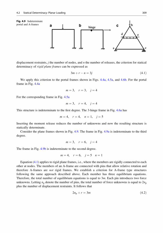
Consider the plane frames shown in Fig. 4.9. The frame in Fig. 4.9a is indeterminate to the third
degree.
m ¼ 3, r ¼ 6, j ¼ 4
The frame in Fig. 4.9b is indeterminate to the second degree.
m ¼ 4, r ¼ 6, j ¼ 5 n ¼ 1
Equation (4.1) applies to rigid plane frames, i.e., where the members are rigidly connected to each
other at nodes. The members of an A-frame are connected with pins that allow relative rotation and
therefore A-frames are not rigid frames. We establish a criterion for A-frame type structures
following the same approach described above. Each member has three equilibrium equations.
Therefore, the total number of equilibrium equations is equal to 3m. Each pin introduces two force
unknowns. Letting np denote the number of pins, the total number of force unknowns is equal to 2npplus the number of displacement restraints. It follows that
2np þ r ¼ 3m ð4:2Þ
Fig. 4.9 Indeterminate
portal and A-frames
4.2 Statical Determinacy: Planar Loading 309
for static determinacy of A-frame type structures. Applying this criterion to the structure shown in
Fig. 4.2, one has np ¼ 3, r ¼ 3, m ¼ 3, and the structure is statically determinate. If we add another
member at the base, as shown in Fig. 4.9c, np ¼ 5, r ¼ 3, m ¼ 4, and the structure becomes statically
indeterminate to the first degree.
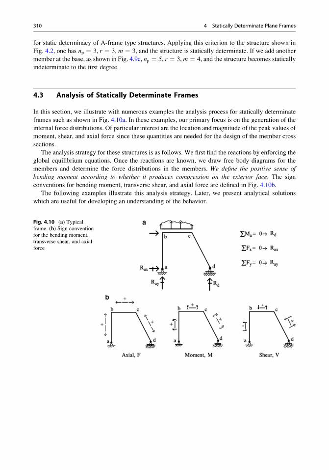
4.3 Analysis of Statically Determinate Frames
In this section, we illustrate with numerous examples the analysis process for statically determinate
frames such as shown in Fig. 4.10a. In these examples, our primary focus is on the generation of the
internal force distributions. Of particular interest are the location and magnitude of the peak values of
moment, shear, and axial force since these quantities are needed for the design of the member cross
sections.
The analysis strategy for these structures is as follows. We first find the reactions by enforcing the
global equilibrium equations. Once the reactions are known, we draw free body diagrams for the
members and determine the force distributions in the members. We define the positive sense of
bending moment according to whether it produces compression on the exterior face. The sign
conventions for bending moment, transverse shear, and axial force are defined in Fig. 4.10b.
The following examples illustrate this analysis strategy. Later, we present analytical solutions
which are useful for developing an understanding of the behavior.
Fig. 4.10 (a) Typicalframe. (b) Sign convention
for the bending moment,
transverse shear, and axial
force
310 4 Statically Determinate Plane Frames
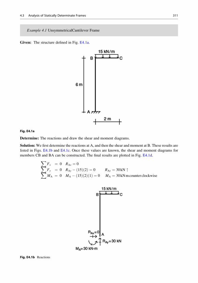
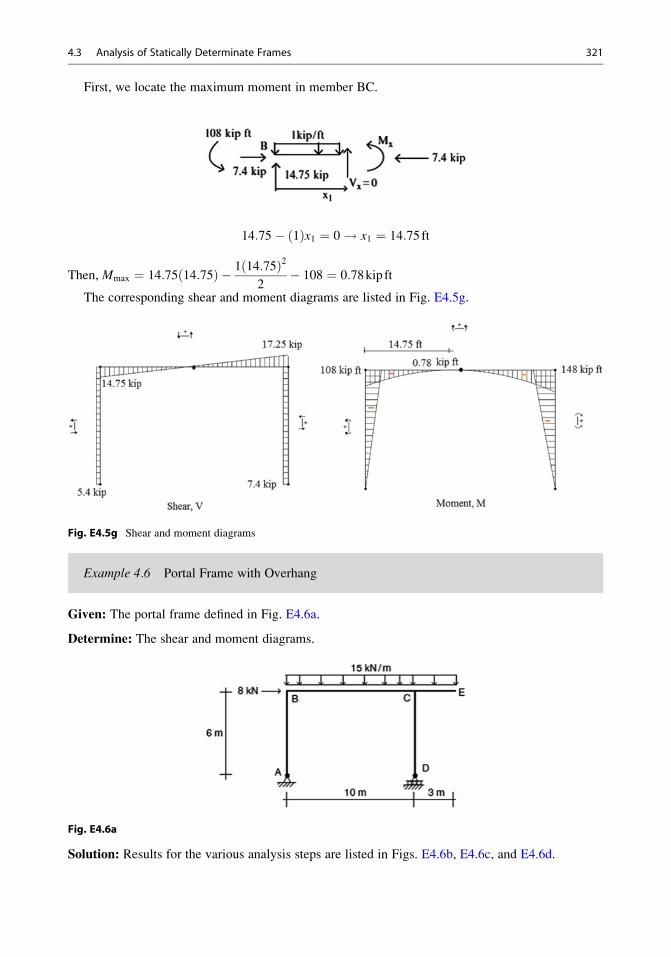
Example 4.1 UnsymmetricalCantilever Frame
Given: The structure defined in Fig. E4.1a.
Fig. E4.1a
Determine: The reactions and draw the shear and moment diagrams.
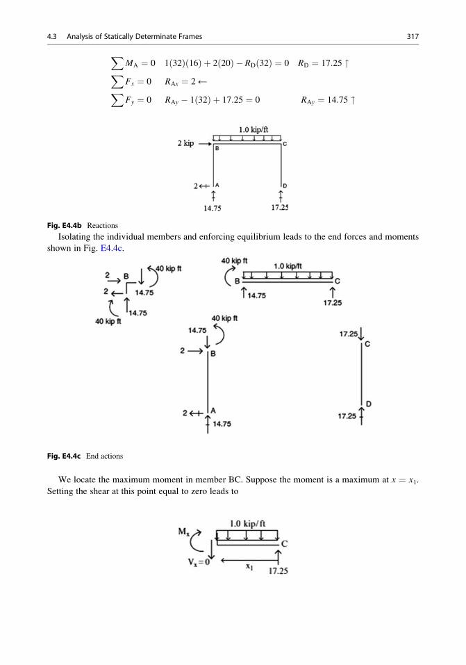
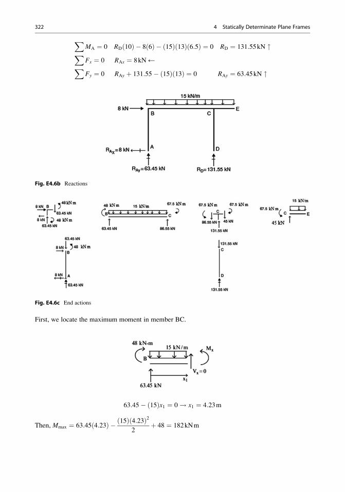
Solution:We first determine the reactions at A, and then the shear and moment at B. These results are
listed in Figs. E4.1b and E4.1c. Once these values are known, the shear and moment diagrams for
members CB and BA can be constructed. The final results are plotted in Fig. E4.1d.XFx ¼ 0 RAx ¼ 0XFy ¼ 0 RAy � 15ð Þ 2ð Þ ¼ 0 RAy ¼ 30kN "XMA ¼ 0 MA � 15ð Þ 2ð Þ 1ð Þ ¼ 0 MA ¼ 30kNmcounter clockwise
Fig. E4.1b Reactions
4.3 Analysis of Statically Determinate Frames 311
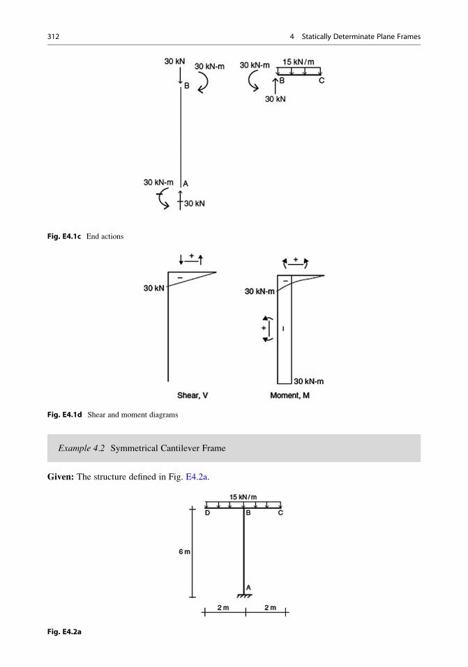
Fig. E4.1c End actions
Fig. E4.1d Shear and moment diagrams
Example 4.2 Symmetrical Cantilever Frame
Given: The structure defined in Fig. E4.2a.
Fig. E4.2a
312 4 Statically Determinate Plane Frames
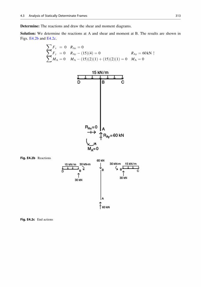
Determine: The reactions and draw the shear and moment diagrams.
Solution: We determine the reactions at A and shear and moment at B. The results are shown in
Figs. E4.2b and E4.2c.XFx ¼ 0 RAx ¼ 0XFy ¼ 0 RAy � 15ð Þ 4ð Þ ¼ 0 RAy ¼ 60kN "XMA ¼ 0 MA � 15ð Þ 2ð Þ 1ð Þ þ 15ð Þ 2ð Þ 1ð Þ ¼ 0 MA ¼ 0
Fig. E4.2b Reactions
Fig. E4.2c End actions
4.3 Analysis of Statically Determinate Frames 313
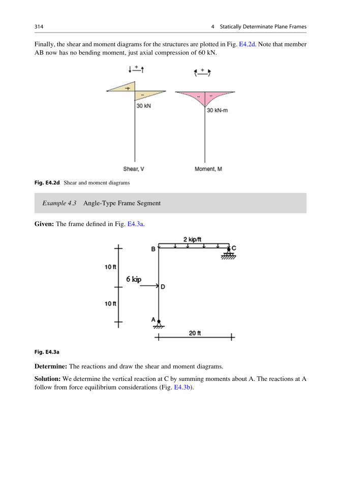
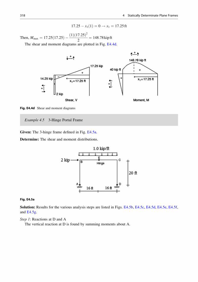
Finally, the shear and moment diagrams for the structures are plotted in Fig. E4.2d. Note that member
AB now has no bending moment, just axial compression of 60 kN.
Fig. E4.2d Shear and moment diagrams
Example 4.3 Angle-Type Frame Segment
Given: The frame defined in Fig. E4.3a.
Fig. E4.3a
Determine: The reactions and draw the shear and moment diagrams.
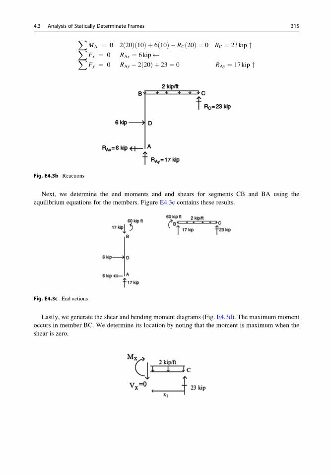
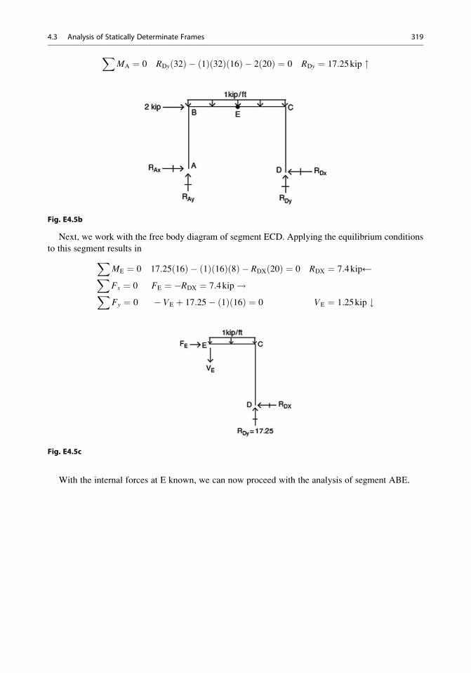
Solution:We determine the vertical reaction at C by summing moments about A. The reactions at A
follow from force equilibrium considerations (Fig. E4.3b).
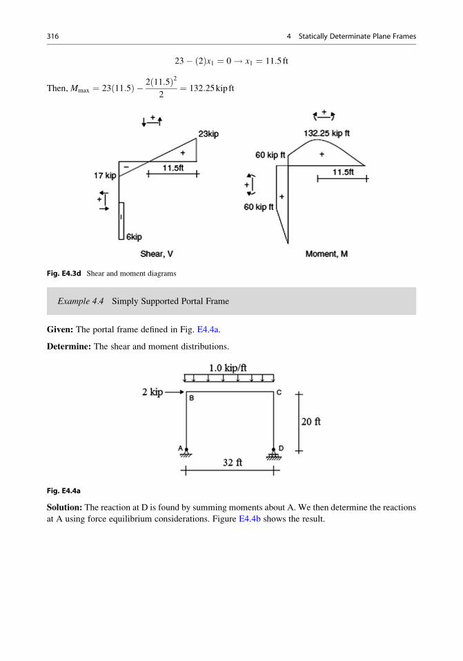
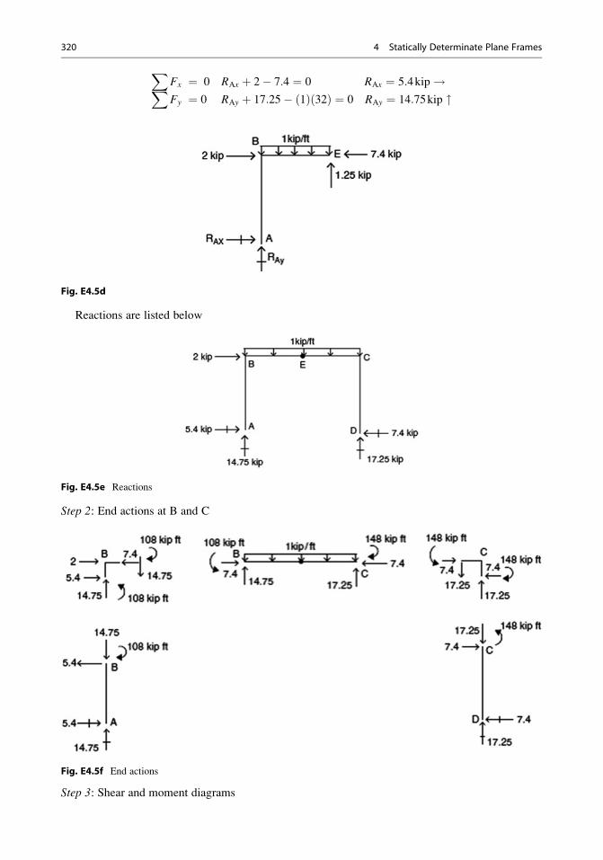
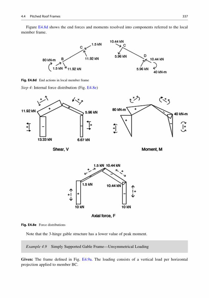
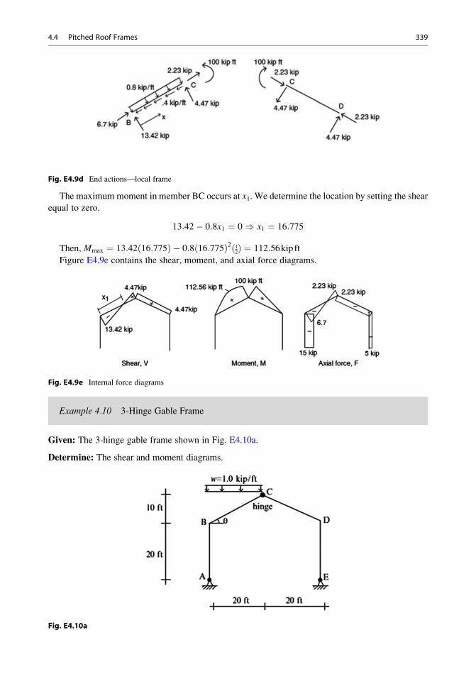
Figure E4.9e contains the shear, moment, and axial force diagrams.
Fig. E4.9e Internal force diagrams
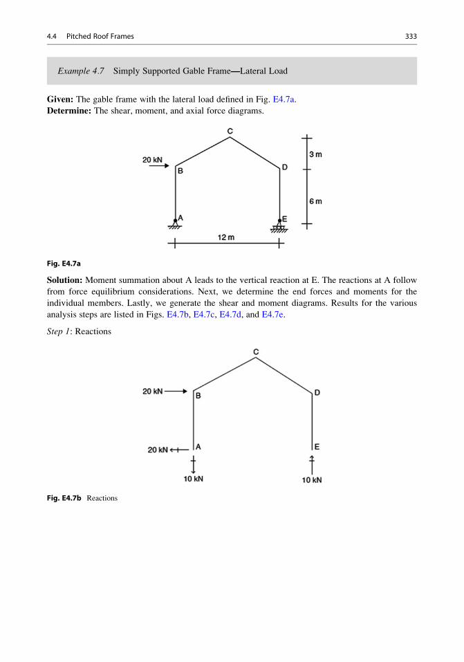
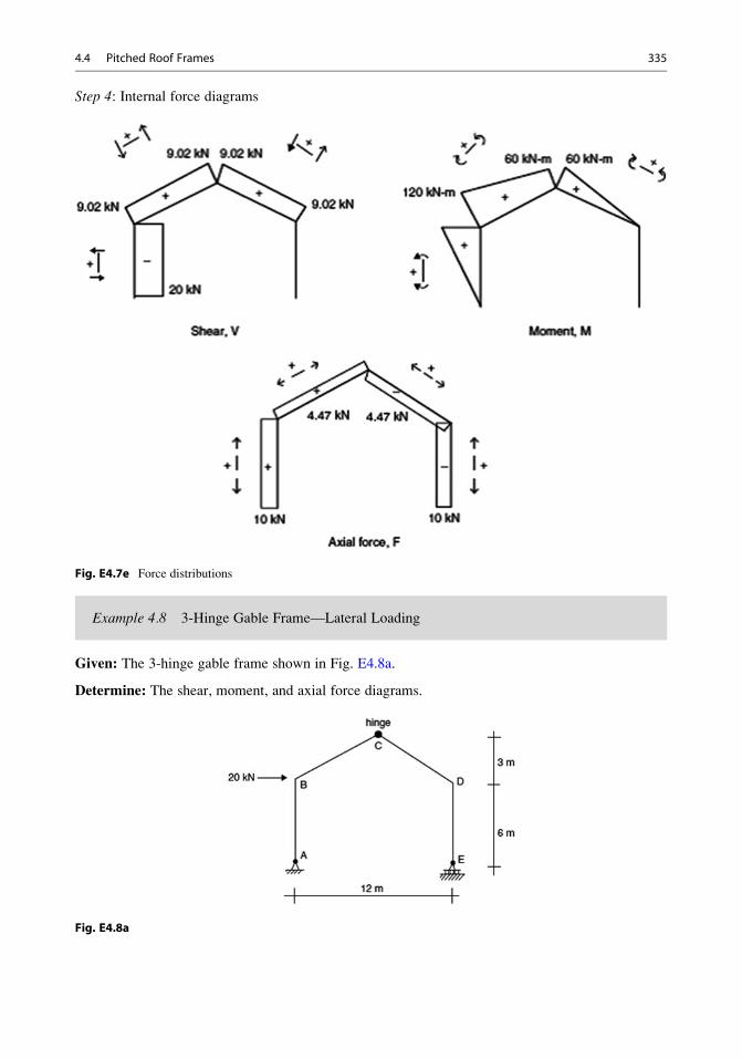
Example 4.10 3-Hinge Gable Frame
Given: The 3-hinge gable frame shown in Fig. E4.10a.
Determine: The shear and moment diagrams.
Fig. E4.10a
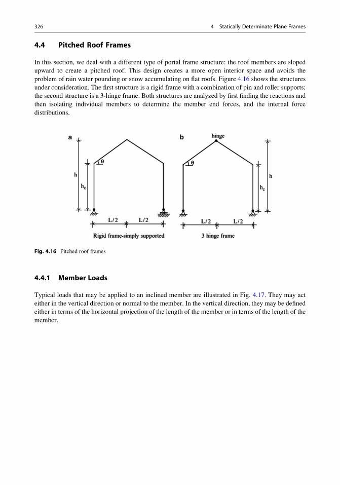
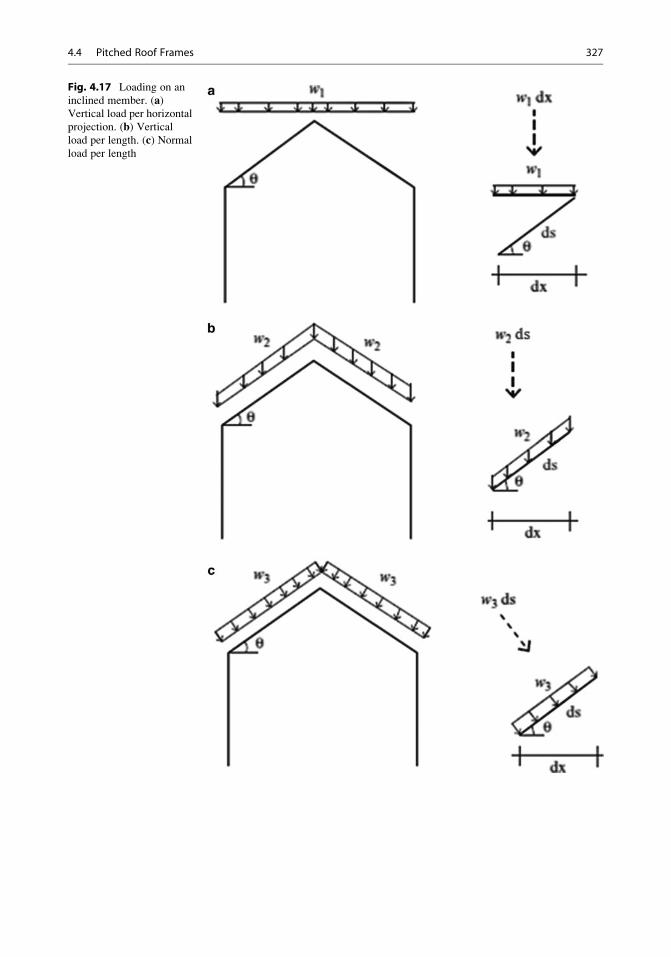
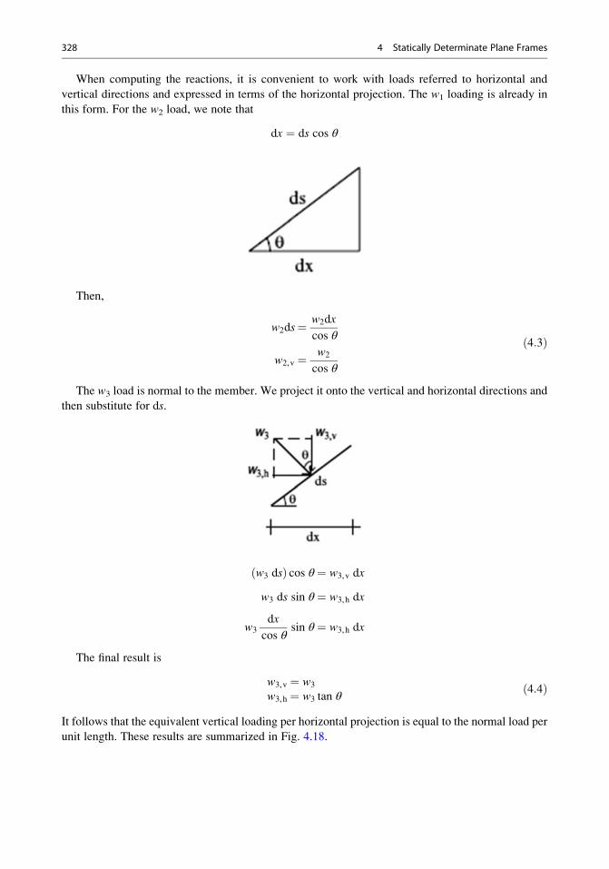
4.4 Pitched Roof Frames 339
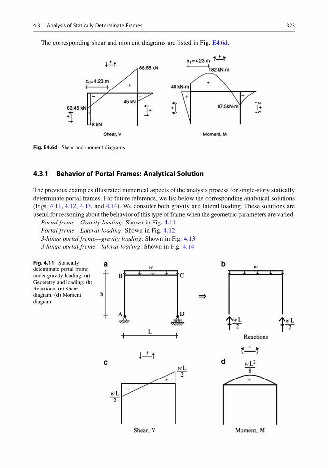
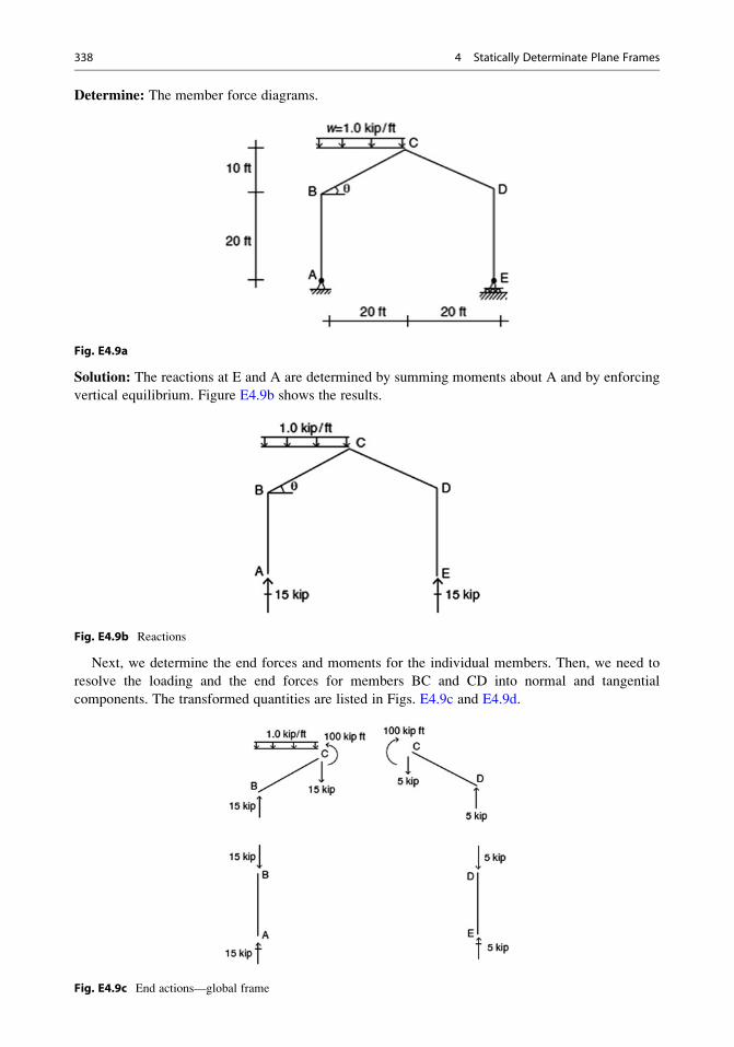
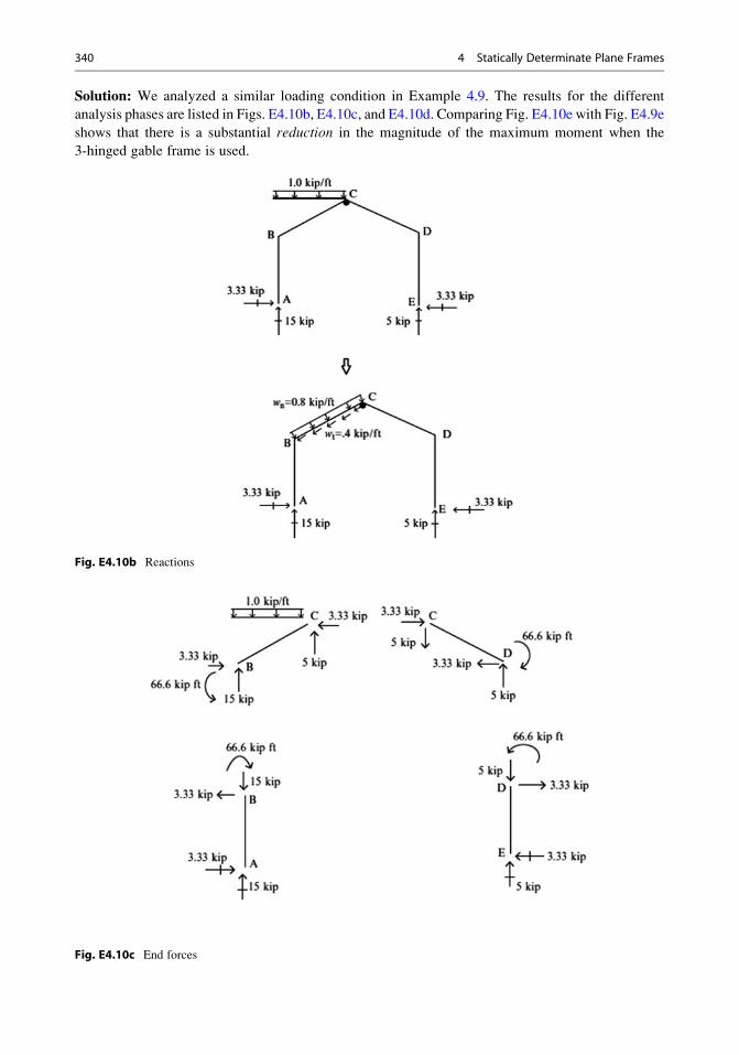
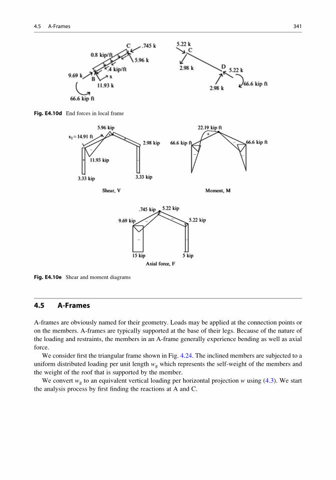
Solution: We analyzed a similar loading condition in Example 4.9. The results for the different
analysis phases are listed in Figs. E4.10b, E4.10c, and E4.10d. Comparing Fig. E4.10e with Fig. E4.9e
shows that there is a substantial reduction in the magnitude of the maximum moment when the
3-hinged gable frame is used.
Fig. E4.10b Reactions
Fig. E4.10c End forces
340 4 Statically Determinate Plane Frames
Fig. E4.10d End forces in local frame
Fig. E4.10e Shear and moment diagrams
4.5 A-Frames
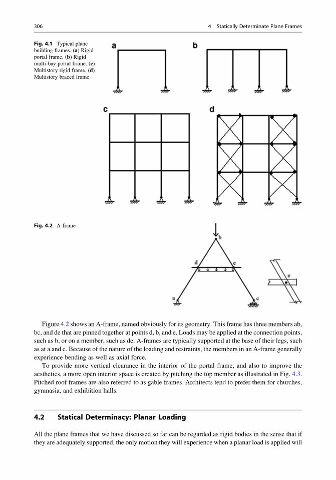
A-frames are obviously named for their geometry. Loads may be applied at the connection points or
on the members. A-frames are typically supported at the base of their legs. Because of the nature of
the loading and restraints, the members in an A-frame generally experience bending as well as axial
force.
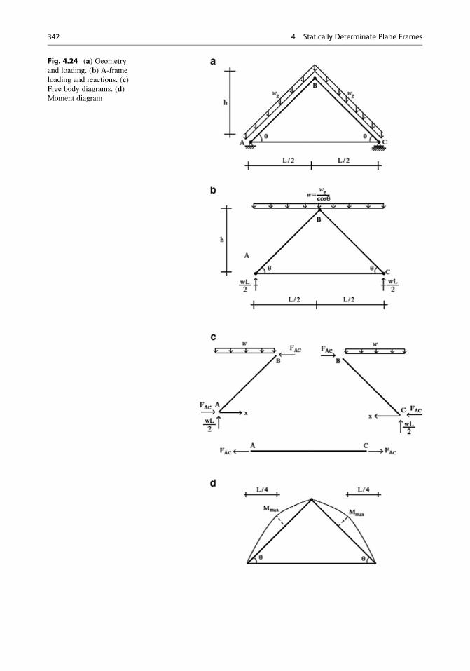
We consider first the triangular frame shown in Fig. 4.24. The inclined members are subjected to a
uniform distributed loading per unit length wg which represents the self-weight of the members and
the weight of the roof that is supported by the member.
We convert wg to an equivalent vertical loading per horizontal projection w using (4.3). We start
the analysis process by first finding the reactions at A and C.
4.5 A-Frames 341
Fig. 4.24 (a) Geometry
and loading. (b) A-frame
loading and reactions. (c)Free body diagrams. (d)Moment diagram
342 4 Statically Determinate Plane Frames
Next, we isolate member BC (see Fig. 4.24c).
XMat B ¼ �w
2
L
2
� �2
þ wL
2
L
2
� �� hFAC ¼ 0
+
FAC ¼ wL2
8h
The horizontal internal force at B must equilibrate FAC. Lastly, we determine the moment
distribution in members AB and BC. Noting Fig. 4.24c, the bending moment at location x is given by
M xð Þ ¼ wL
2x� FAC
2h
L
� �x� wx2
2¼ wL
4x� wx2
2
The maximum moment occurs at x ¼ L/4 and is equal to
Mmax ¼ wL2
32
Replacing w with wg, we express Mmax as
Mmax ¼ wg
cos θ
� � L2
32
As θ increases, the moment increases even though the projected length of the member remains
constant.
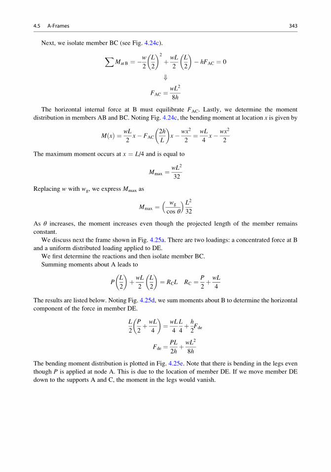
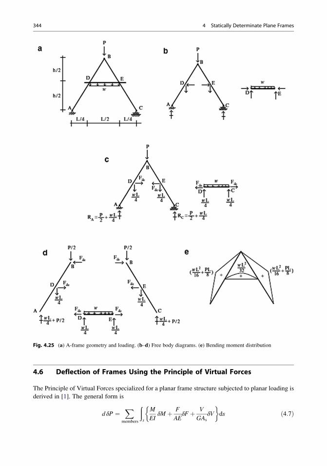
We discuss next the frame shown in Fig. 4.25a. There are two loadings: a concentrated force at B
and a uniform distributed loading applied to DE.
We first determine the reactions and then isolate member BC.
Summing moments about A leads to
PL
2
� �þ wL
2
L
2
� �¼ RCL RC ¼ P
2þ wL
4
The results are listed below. Noting Fig. 4.25d, we sum moments about B to determine the horizontal
component of the force in member DE.
L
2
P
2þ wL
4
� �¼ wL
4
L
4þ h
2Fde
Fde ¼ PL
2hþ wL2
8h
The bending moment distribution is plotted in Fig. 4.25e. Note that there is bending in the legs even
though P is applied at node A. This is due to the location of member DE. If we move member DE
down to the supports A and C, the moment in the legs would vanish.
4.5 A-Frames 343
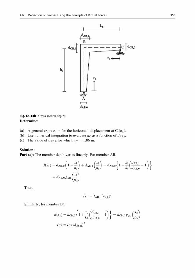
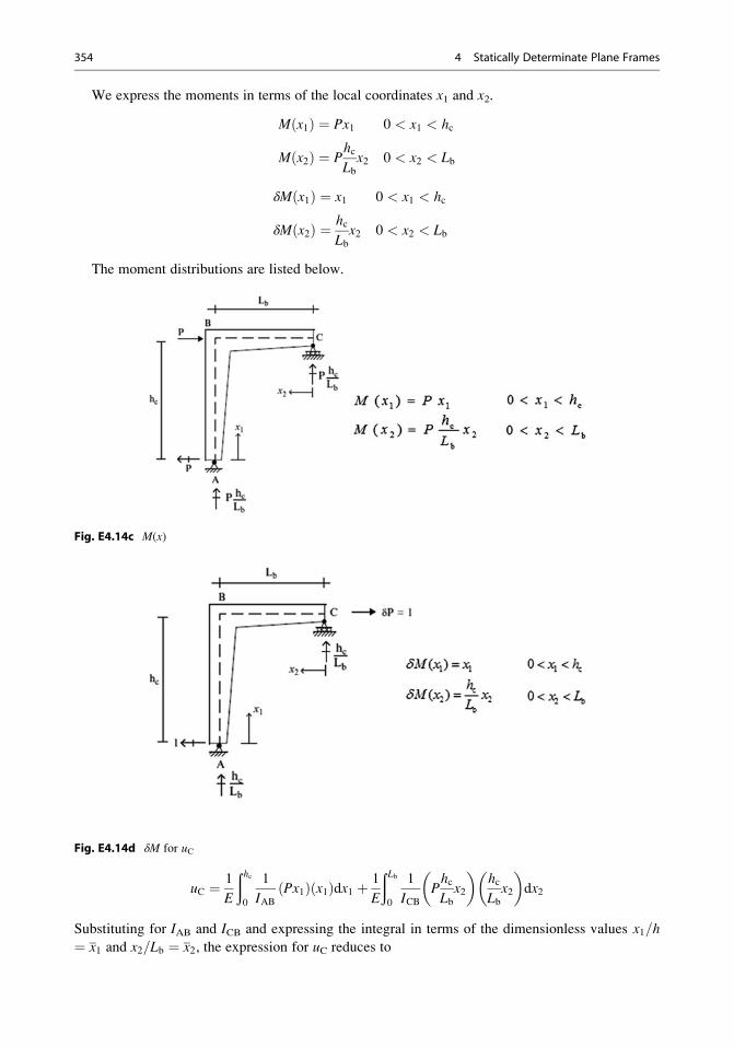
4.6 Deflection of Frames Using the Principle of Virtual Forces
The Principle of Virtual Forces specialized for a planar frame structure subjected to planar loading is
derived in [1]. The general form is
d δP ¼X
members
ðs
M
EIδM þ F
AEδFþ V
GAs
δV
� �ds ð4:7Þ
Fig. 4.25 (a) A-frame geometry and loading. (b–d) Free body diagrams. (e) Bending moment distribution
344 4 Statically Determinate Plane Frames
Frames carry loading primarily by bending action. Axial and shear forces are developed as a result of
the bending action, but the contribution to the displacement produced by shear deformation is generally
small in comparison to the displacement associated with bending deformation and axial deformation.
Therefore, we neglect this term and work with a reduced form of the principle of Virtual Forces.
d δP ¼X
members
ðs
M
EIδM þ F
AEδF
� �ds ð4:8Þ
where δP is either a unit force (for displacement) or a unit moment (for rotation) in the direction of the
desired displacement d; δM, and δF are the virtual moment and axial force due to δP. The integrationis carried out over the length of each member and then summed up.
For low-rise frames, i.e., where the ratio of height to width is on the order of unity, the axial
deformation term is also small. In this case, one neglects the axial deformation term in (4.8) and
works with the following form
d δP ¼X
members
ðs
M
EI
� �δMð Þds ð4:9Þ
Axial deformation is significant for tall buildings, and (4.8) is used for this case. In what follows,
we illustrate the application of the Principle of Virtual Forces to some typical low-rise structures. We
revisit this topic later in Chap. 9, which deals with statically indeterminate frames.
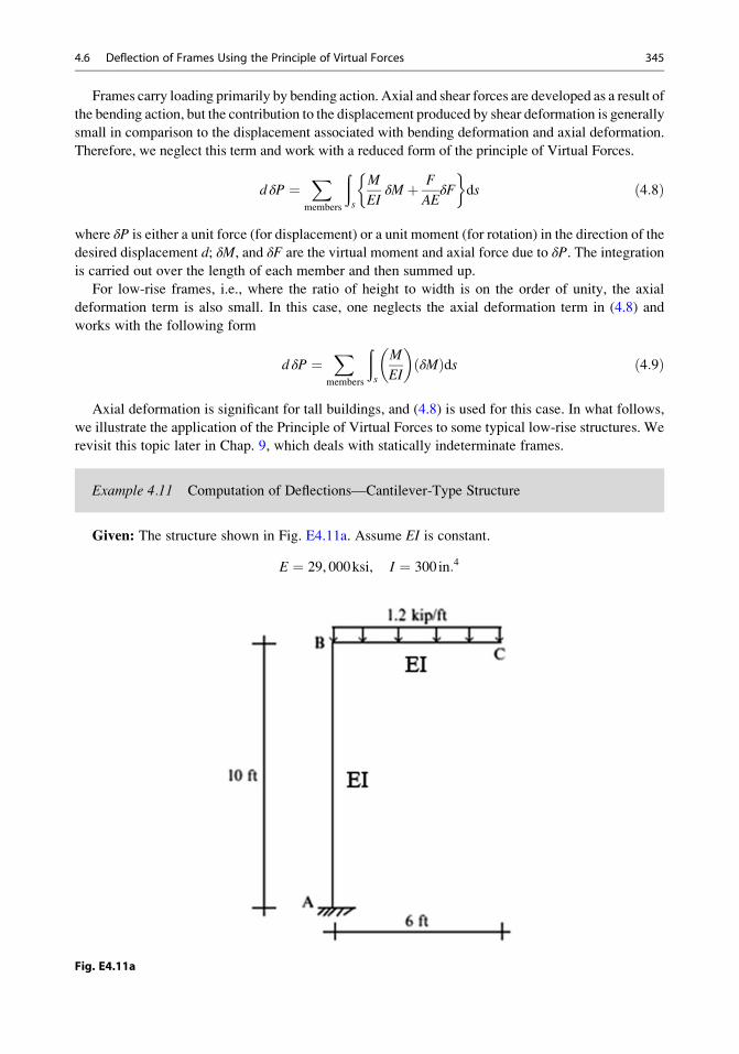
Example 4.11 Computation of Deflections—Cantilever-Type Structure
Given: The structure shown in Fig. E4.11a. Assume EI is constant.
E ¼ 29, 000ksi, I ¼ 300 in:4
Fig. E4.11a
4.6 Deflection of Frames Using the Principle of Virtual Forces 345
Determine: The horizontal and vertical deflections and the rotation at point C, the tip of the cantilever
segment.
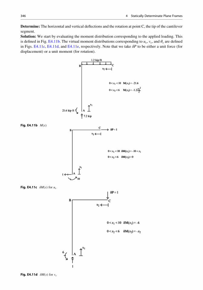
Solution: We start by evaluating the moment distribution corresponding to the applied loading. This
is defined in Fig. E4.11b. The virtual moment distributions corresponding to uc, vc, and θc are definedin Figs. E4.11c, E4.11d, and E4.11e, respectively. Note that we take δP to be either a unit force (for
displacement) or a unit moment (for rotation).
Fig. E4.11b M(x)
Fig. E4.11c δM(x) for uc
Fig. E4.11d δM(x) for vc
346 4 Statically Determinate Plane Frames
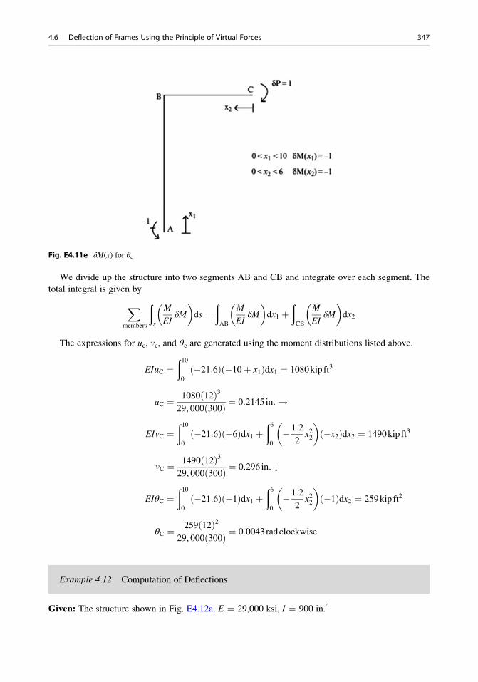
Fig. E4.11e δM(x) for θc
We divide up the structure into two segments AB and CB and integrate over each segment. The
total integral is given by
Xmembers
ðs
M
EIδM
� �ds ¼
ðAB
M
EIδM
� �dx1 þ
ðCB
M
EIδM
� �dx2
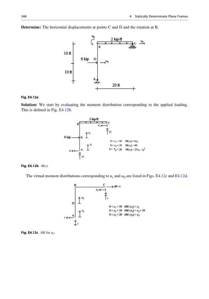
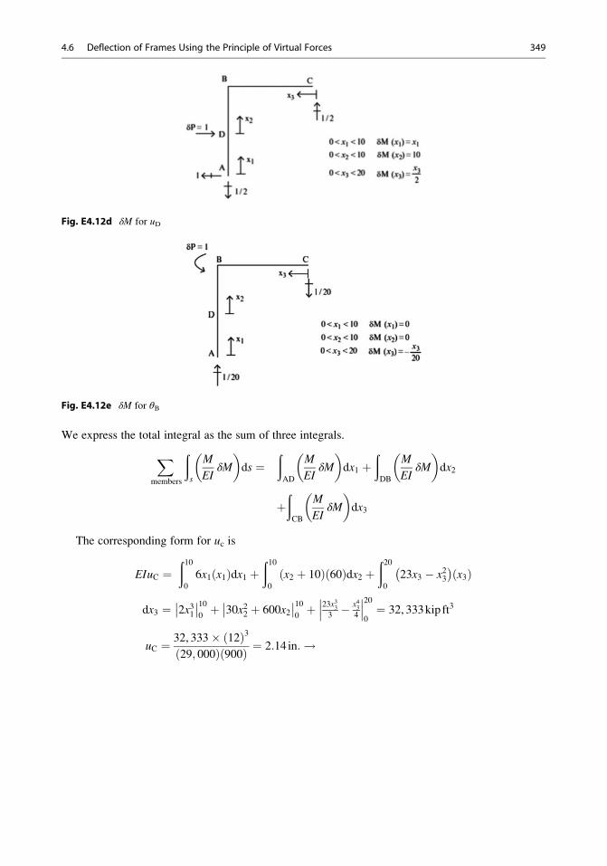
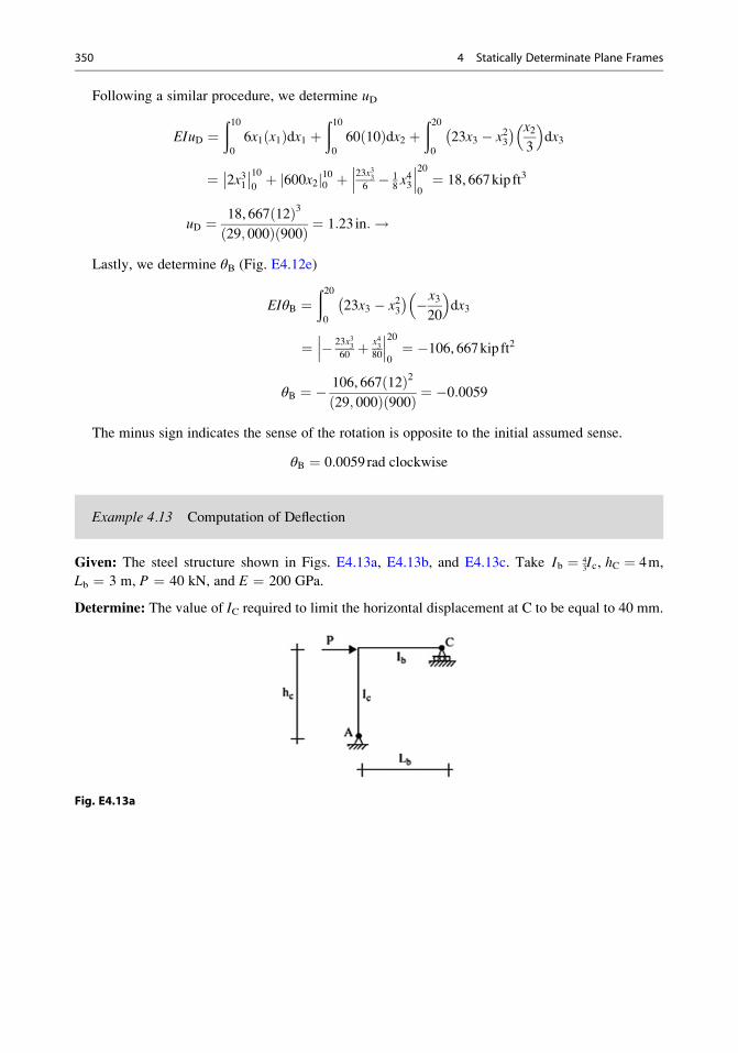
The expressions for uc, vc, and θc are generated using the moment distributions listed above.