SCIENCE Statistical analysis of flashover data using a generalised likelihood method A.J. Davies, BSc, PhD, CEng, FIEE A.R. Rowlands, BEng(Tech), BA, DipEE, CEng R. Turri, Dott Ing Prof. R.T. Waters, BSc, PhD, CEng, FIEE Indexing terms: Arcing, Breakdown and gas discharge Abstract: In order to ensure consistency in the treatment of flashover data, it is desirable that a standard method of analysis of test results be established. Previous workers have suggested that the maximum likelihood method would be appro- priate for estimating the parameters of the break- down probability distribution, such as V 50 and a in the normal distribution. The present paper shows how this method may be applied in practice and can be extended to determine the confidence region associated with sets of parameters, and the confidence interval on a single parameter. It is also shown how other parameters, such as the voltage level corresponding to a specified prob- ability of breakdown, may be determined. An example is given of the application of the method to a typical data set for flashover in air together with a listing of a suitable computer program in Fortran 77. It is recommended that this method be considered for adoption as a standard pro- cedure. 1 Introduction A variety of different test strategies may be employed in investigating the breakdown characteristics of a discharge gap subjected to impulse voltages. In the Class I multilevel test procedure [1], for example, a number of impulses are applied for a fixed value of the crest voltage and the number of breakdown and withstand events recorded. The time between the voltage applications must be sufficient for each applica- tion to be independent (i.e. the same initial conditions apply) and the test is repeated for various crest voltages in the region where the breakdown probability undergoes a transition from a low to a high value. In analysing the results of such tests it is normally desired to evaluate the crest voltage V 50 at which there is a 50% probability of flashover and also some measure of the range of voltages over which the probability of break- Paper 5723A (S3), first received 21st November 1986 and in revised form 21st July 1987 Dr. Davies and Dr. Turn are with the Department of Physics, Uni- versity College of Swansea, Singleton Park, Swansea SA2 8PP, United Kingdom Prof. Waters and Mr. Rowlands are with the Department of Physics, Electronics & Electrical Engineering, University of Wales Institute of Science and Technology, PO Box 25, Cardiff CF1 3XE, United Kingdom down P B (V) increases from very low to very high values (Fig. la). Most workers in the past have taken the form of the distribution of Fig. la to be that of the cumulative 100 o o. 50 16 80 86 92 98 crest voltage, kV 104 110 0.01 80 104 86 92 98 crest voltage , kV b Fig. 1 Typical breakdown probability distribution on linear axes (a) and cumulative normal probability paper \b) A = observed frequencies of breakdown (data of Table 2) IEE PROCEEDINGS, Vol. 135, Pt. A, No. 1, JANUARY 1988 79
Transcript
SCIENCE
Statistical analysis of flashover data using ageneralised likelihood method
Indexing terms: Arcing, Breakdown and gas discharge
Abstract: In order to ensure consistency in thetreatment of flashover data, it is desirable that astandard method of analysis of test results beestablished. Previous workers have suggested thatthe maximum likelihood method would be appro-priate for estimating the parameters of the break-down probability distribution, such as V50 and ain the normal distribution. The present papershows how this method may be applied in practiceand can be extended to determine the confidenceregion associated with sets of parameters, and theconfidence interval on a single parameter. It isalso shown how other parameters, such as thevoltage level corresponding to a specified prob-ability of breakdown, may be determined. Anexample is given of the application of the methodto a typical data set for flashover in air togetherwith a listing of a suitable computer program inFortran 77. It is recommended that this methodbe considered for adoption as a standard pro-cedure.
1 Introduction
A variety of different test strategies may be employed ininvestigating the breakdown characteristics of a dischargegap subjected to impulse voltages.
In the Class I multilevel test procedure [1], forexample, a number of impulses are applied for a fixedvalue of the crest voltage and the number of breakdownand withstand events recorded. The time between thevoltage applications must be sufficient for each applica-tion to be independent (i.e. the same initial conditionsapply) and the test is repeated for various crest voltagesin the region where the breakdown probability undergoesa transition from a low to a high value.
In analysing the results of such tests it is normallydesired to evaluate the crest voltage V50 at which there isa 50% probability of flashover and also some measure ofthe range of voltages over which the probability of break-Paper 5723A (S3), first received 21st November 1986 and in revised
form 21st July 1987Dr. Davies and Dr. Turn are with the Department of Physics, Uni-versity College of Swansea, Singleton Park, Swansea SA2 8PP, UnitedKingdomProf. Waters and Mr. Rowlands are with the Department of Physics,Electronics & Electrical Engineering, University of Wales Institute ofScience and Technology, PO Box 25, Cardiff CF1 3XE, UnitedKingdom
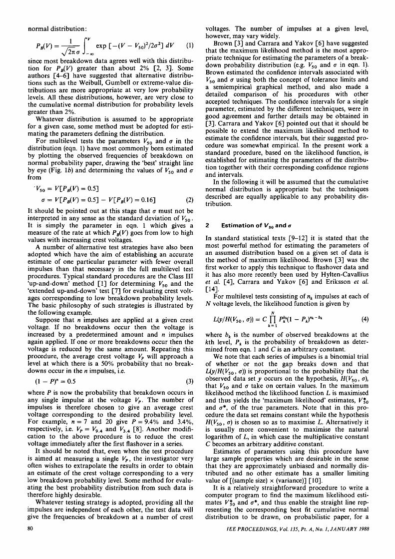
down PB(V) increases from very low to very high values(Fig. la).
Most workers in the past have taken the form of thedistribution of Fig. la to be that of the cumulative
100
oo. 50
16
80 86 92 98
crest voltage, kV
104 110
0.01
80 10486 92 98
crest voltage , kV
b
Fig. 1 Typical breakdown probability distribution on linear axes (a)and cumulative normal probability paper \b)A = observed frequencies of breakdown (data of Table 2)
IEE PROCEEDINGS, Vol. 135, Pt. A, No. 1, JANUARY 1988 79
normal distribution:
=—r (1)
since most breakdown data agrees well with this distribu-tion for PB(V) greater than about 2% [2, 3]. Someauthors [4-6] have suggested that alternative distribu-tions such as the Weibull, Gumbell or extreme-value dis-tributions are more appropriate at very low probabilitylevels. All these distributions, however, are very close tothe cumulative normal distribution for probability levelsgreater than 2%.
Whatever distribution is assumed to be appropriatefor a given case, some method must be adopted for esti-mating the parameters defining the distribution.
For multilevel tests the parameters Vso and a in thedistribution (eqn. 1) have most commonly been estimatedby plotting the observed frequencies of breakdown onnormal probability paper, drawing the 'best' straight lineby eye (Fig. \b) and determining the values of V50 and afrom
'^50 = VIPB(V) = 0.5]
o = V[PB(V) = 0.5] - V[_PB{V) = 0.16] (2)
It should be pointed out at this stage that a must not beinterpreted in any sense as the standard deviation of V50.It is simply the parameter in eqn. 1 which gives ameasure of the rate at which PB(V) goes from low to highvalues with increasing crest voltages.
A number of alternative test strategies have also beenadopted which have the aim of establishing an accurateestimate of one particular parameter with fewer overallimpulses than that necessary in the full multilevel testprocedures. Typical standard procedures are the Class III'up-and-down' method [1] for determining V50 and the'extended up-and-down' test [7] for evaluating crest volt-ages corresponding to low breakdown probability levels.The basic philosophy of such strategies is illustrated bythe following example.
Suppose that n impulses are applied at a given crestvoltage. If no breakdowns occur then the voltage isincreased by a predetermined amount and n impulsesagain applied. If one or more breakdowns occur then thevoltage is reduced by the same amount. Repeating thisprocedure, the average crest voltage VP will approach alevel at which there is a 50% probability that no break-downs occur in the n impulses, i.e.
(1 - P)n = 0.5 (3)
where P is now the probability that breakdown occurs inany single impulse at the voltage VP. The number ofimpulses is therefore chosen to give an average crestvoltage corresponding to the desired probability level.For example, n = 7 and 20 give P = 9.4% and 3.4%,respectively, i.e. VP = V9 4 and V3A [8]. Another modifi-cation to the above procedure is to reduce the crestvoltage immediately after the first flashover in a series.
It should be noted that, even when the test procedureis aimed at measuring a single VP, the investigator veryoften wishes to extrapolate the results in order to obtainan estimate of the crest voltage corresponding to a verylow breakdown probability level. Some method for evalu-ating the best probability distribution from such data istherefore highly desirable.
Whatever testing strategy is adopted, providing all theimpulses are independent of each other, the test data willgive the frequencies of breakdown at a number of crest
voltages. The number of impulses at a given level,however, may vary widely.
Brown [3] and Carrara and Yakov [6] have suggestedthat the maximum likelihood method is the most appro-priate technique for estimating the parameters of a break-down probability distribution (e.g. V50 and a in eqn. 1).Brown estimated the confidence intervals associated withV50 and a using both the concept of tolerance limits anda semiempirical graphical method, and also made adetailed comparison of his procedures with otheraccepted techniques. The confidence intervals for a singleparameter, estimated by the different techniques, were ingood agreement and further details may be obtained in[3]. Carrara and Yakov [6] pointed out that it should bepossible to extend the maximum likelihood method toestimate the confidence intervals, but their suggested pro-cedure was somewhat empirical. In the present work astandard procedure, based on the likelihood function, isestablished for estimating the parameters of the distribu-tion together with their corresponding confidence regionsand intervals.
In the following it will be assumed that the cumulativenormal distribution is appropriate but the techniquesdescribed are equally applicable to any probability dis-tribution.
2 Estimation of Vs0 and a
In standard statistical texts [9-12] it is stated that themost powerful method for estimating the parameters ofan assumed distribution based on a given set of data isthe method of maximum likelihood. Brown [3] was thefirst worker to apply this technique to flashover data andit has also more recently been used by Hylten-Cavalliuset al. [4], Carrara and Yakov [6] and Eriksson et al.[14].
For multilevel tests consisting of nk impulses at each ofN voltage levels, the likelihood function is given by
L(y/H{V5Q,a)) = C (4)
where bk is the number of observed breakdowns at thefcth level, Pk is the probability of breakdown as deter-mined from eqn. 1 and C is an arbitrary constant.
We note that each series of impulses is a binomial trialof whether or not the gap breaks down and thatL(y/H(V50, a)) is proportional to the probability that theobserved data set y occurs on the hypothesis, H(V50, a),that V50 and a take on certain values. In the maximumlikelihood method the likelihood function L is maximisedand thus yields the 'maximum likelihood' estimates, V*o
and a*, of the true parameters. Note that in this pro-cedure the data set remains constant while the hypothesisHiYso* °) 1S chosen so as to maximise L. Alternatively itis usually more convenient to maximise the naturallogarithm of L, in which case the multiplicative constantC becomes an arbitrary additive constant.
Estimates of parameters using this procedure havelarge sample properties which are desirable in the sensethat they are approximately unbiased and normally dis-tributed and no other estimate has a smaller limitingvalue of [(sample size) x (variance)] [10].
It is a relatively straightforward procedure to write acomputer program to find the maximum likelihood esti-mates V%0 and a*, and thus enable the straight line rep-resenting the corresponding best fit cumulative normaldistribution to be drawn, on probabilistic paper, for a
80 IEE PROCEEDINGS, Vol. 135, Pt. A, No. 1, JANUARY 1988
given data set. A listing of a simple algorithm in Fortran77 is given in Appendix 7.3.
A measure of how well the estimated distribution fitsthe observed breakdown frequencies can be obtainedfrom a x-square test which, for example, in the multilevelprocedure takes the form [3]
where the Pks are obtained from eqn. 1 with V50 = Kf0and a = cr*. The number of degrees of freedom isy = N — 2 and the parameter h = x2/y is expected to beof order of, or less than, unity. Values of h appreciablygreater than 1 either indicate that the assumed distribu-tion is inappropriate, or that a particular data set maynot be reliable and that care must be taken in inter-preting the results.
In any testing it would seem highly desirable to carryout a x-square check oh the results as they are taken inorder to verify that consistent data have been obtained.
3 Confidence region and confidence intervals
In his studies Brown [3] compared several differentmethods, all based on the concept of variances, for esti-mating the confidence interval associated with a singledistribution parameter. Carrara and Yakov [6] pointedout that the likelihood approach could be extended todetermine the confidence region associated with thesimultaneous evaluation of the distribution parameters.They concluded, however, that further work was neces-sary to put their semiempirical procedure on to a soundstatistical basis.
In the following it is shown how the likelihood func-tion may be used to estimate both the confidence regionand confidence intervals associated with the maximumlikelihood estimates evaluated as in Section 2.
3.1 The confidence region for V%0 and a*The P% confidence region for the maximum likelihoodestimators V%0 and a* is defined by the boundary in theV50/cr plane for which there is a P% probability that thetrue values of V50 and a lie within this boundary. It canbe demonstrated [10-12] that the inequality
Uy/H(V50,a))Ky/H(V*50,o*)) > K (6)
defines the 100(1 — a) per cent confidence region for thehypothesis H(V%0, a*), provided that the constant K ischosen to correspond to a confidence level of the likeli-hood ratio (i.e. the left-hand side of eqn. 6) equal to(1 - a).
The determination of K is not straightforward and in[6], for example, it was suggested on semiempiricalgrounds that a value of K equal to 0.2 was appropriatefor a 90% confidence region. There is, however, a wellestablished theorem [12, 13] that in the limit of largesamples
2[ln Uy/H*) - In Uy/H)] (7)
may be approximated by a limiting /-square distributionX2(r) with a degree of freedom, r, equal to the number ofparameters in the hypothesis H. If we denote by C(a) thevalue of x2(r) corresponding to a probability of (1 — a),
the 100(1 — a) per cent confidence region will be given by
< C(a) (8)Uy/H(V50,<j))
that is
UylH{V50,o)) 2
Uy/H(V*0,a*)) (9)
so that K may be identified with the corresponding valueof e~C(a)l2 and is easily calculated from standard x-squaretables.
Table 1 shows the values of K for the 90%, 95% and99% confidence regions at various degrees of freedom.
Table 1 : Values of K in relation (6) corresponding to differ-ent confidence levels (1 - at)
Degrees 90% 95% 99%of freedom r (a = 0.1) (a = 0.05) (a = 0.01)
We thus see that the locus of points in the V50/o planefor which the likelihood ratio is equal to 0.1 defines a90% confidence region for the simultaneous estimatesV%0 and a*. This value of the likelihood ratio was alsoemployed by Eriksson et al. [14]. For large samples thisconfidence region will have an elliptic shape and Fig. 2shows the results obtained for the typical set of flashoverdata, Table 2, taken from experimental results reported in
i 0 r
4.224
92 94 96 98 100 102
V 50 - k V
Fig. 2 Maximum likelihood estimation of V50 ( = 96.92 kV), a( = 4.224 kV) and the associated 90% confidence region for the typicaldata set of Table 2
Table 2: Typical set of flashover data (15]
Crest voltage, kV
8790929496
102
Number of breakdowns(out of 20 impulses)
02158
18
IEE PROCEEDINGS, Vol. 135, Pt. A, No. 1, JANUARY 1988 81
a companion paper [15], in which the generalised likeli-hood method is extensively applied.
3.2 Confidence intervals for the individual parametersV*oanda*
In many circumstances it is more convenient to evaluateconfidence intervals for the individual parameters V%0
and a* since they are more easily presented in tabularform. Brown has, for example, made a detailed exami-nation of the various methods of determining the con-fidence intervals from the variances of the maximumlikelihood estimators of V50 and a [3].
The simplest (and most optimistic) method assumesthat the error in the estimation of a parameter is nor-mally distributed and that the sample is sufficiently largefor tolerance limits to be used. Thus, for example, the100(1 — a)% confidence interval for V%0 is defined by
± (10)
where t is the 100(1 — a)% tolerance limit and vVsQt thevariance of V%0 (see Appendixes 7.1 and 7.2).
It is also possible, however, to estimate the confidenceinterval for a single parameter from the likelihood func-tion [10, 12]. In this case the generalised likelihood ratio[10] must be used since the hypothesis concerning thedistribution and the parameters is composite rather thansimple. A hypothesis is termed simple when it defines thedistribution of the random variable exactly, otherwise itis termed composite. Thus, for example, the hypothesisH(V50, a) of a normal distribution with the parametersequal to certain specific values is simple, whereas thehypothesis H(V50) of a normal distribution with V50
specified but a unspecified is composite.In order to establish a confidence interval for Vf0, the
maximum value of L(y/H(V50)), obtained by varying <r,may be compared with the maximum of the likelihoodfunction Uy/H(V%0, a*)) and the generalised likelihoodratio test becomes
max L(y/H(V50))
L(y/H(V*0,o*)) (11)
where the limiting ^-square distribution for the 2 log-likelihood ratio now has only one degree of freedombecause only one parameter (K50) is being tested.Uy/H(V50)) is now proportional to the probability thatthe given data set y will occur on the hypothesis, H(V50),that V50 takes a particular value with a unspecified andarbitrary.
For one degree of freedom we see from Table 1 that a90% confidence interval would be obtained withK = 0.258, and a 95% confidence interval withK = 0.1465.
The same procedure may be followed to establish anappropriate confidence interval for a.
Table 3: Maximum likelihood estimates and condidenceintervals for the typical data set of Table 2 as computedfrom the variances (a) and the generalised likelihood ratio (b)
Maximum _likelihoodesti maters, —kV a
Confidence intervals, kV
90% 95%
In Table 3 the 90% and 95% confidence intervals ofV*o and a* computed both from the variances and thegeneralised likelihood test are compared and very goodagreement is obtained between the two methods.
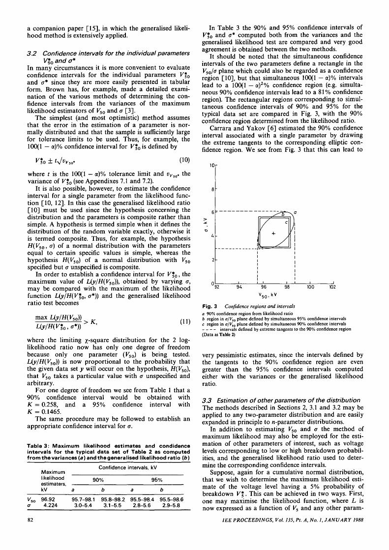
It should be noted that the simultaneous confidenceintervals of the two parameters define a rectangle in theV50/a plane which could also be regarded as a confidenceregion [10], but that simultaneous 100(1 - a)% intervalslead to a 100(1 — a)2% confidence region (e.g. simulta-neous 90% confidence intervals lead to a 81% confidenceregion). The rectangular regions corresponding to simul-taneous confidence intervals of 90% and 95% for thetypical data set are compared in Fig. 3, with the 90%confidence region determined from the likelihood ratio.
Carrara and Yakov [6] estimated the 90% confidenceinterval associated with a single parameter by drawingthe extreme tangents to the corresponding elliptic con-fidence region. We see from Fig. 3 that this can lead to
Fig. 3 Confidence regions and intervalsa 90% confidence region from likelihood ratiob region in o/V50 plane defined by simultaneous 95% confidence intervalsc region in a/V}0 plane defined by simultaneous 90% confidence intervals
intervals defined by extreme tangents to the 90% confidence region(Data as Table 2)
very pessimistic estimates, since the intervals defined bythe tangents to the 90% confidence region are evengreater than the 95% confidence intervals computedeither with the variances or the generalised likelihoodratio.
3.3 Estimation of other parameters of the distributionThe methods described in Sections 2, 3.1 and 3.2 may beapplied to any two-parameter distribution and are easilyexpanded in principle to n-parameter distributions.
In addition to estimating V50 and a the method ofmaximum likelihood may also be employed for the esti-mation of other parameters of interest, such as voltagelevels corresponding to low or high breakdown probabil-ities, and the generalised likelihood ratio used to deter-mine the corresponding confidence intervals.
Suppose, again for a cumulative normal distribution,that we wish to determine the maximum likelihood esti-mate of the voltage level having a 5% probability ofbreakdown V%. This can be achieved in two ways. First,one may maximise the likelihood function, where L isnow expressed as a function of V5 and any other param-
82 IEE PROCEEDINGS, Vol. 135, Pt. A, No. 1, JANUARY 1988
eter, e.g. a. In this case L can be written
L(y/H(V5 ,a)) = CY\ Pbk\l - PJ*-* (12)
where Pk is given by
J2na Jexp {{V - (V5 + 1.65a)]2/2(72} dV (13)
Alternatively, since the cumulative normal distributionhas been assumed to represent the data, V% may be com-puted from
V* = Vtn - 1.65a*50 (14)
provided that Kf0 and a* have already been determined.It can easily be demonstrated that both these pro-
cedures lead to the same value of V% and that themaximum value of the likelihood function is also thesame.
The confidence intervals associated with Vs can beestimated from the generalised likelihood ratio whichnow becomes
max L(y/H(V5))Uy/H(V*0,a*))
>K (15)
where the limiting x-square distribution has one degree offreedom. Table 4 shows the maximum likelihood estima-
Table4: Confidence intervals associated with variousvoltage levels as found from (a) variances and (b) gener-alised likelihood ratio. Data as in Table 2
tes of several voltage levels at high and low breakdownprobabilities together with the 90% confidence intervalsdetermined both from eqn. 15 and from using the conceptof tolerance limits [3] for the assumed data set of Table2.
Very good agreement is obtained between the twoprocedures, but it should be noted that the use of toler-ance limits implies the assumption of a normally distrib-uted error in the estimates (which, however, is usually agood assumption) and large samples, while use of thegeneralised likelihood ratio requires only large samples.
In principle the above method could be used to esti-mate the voltage levels, confidence regions and intervalsassociated with any breakdown probability. It should beremembered, however, that the form of the probabilitydistribution function must be specified and that extrapo-lation to very low or very high breakdown probabilitylevels can only be carried out reliably provided that theassumed distribution remains valid at these levels.
Following the procedure adopted by Brown [3], it isalso possible to estimate from the given data set the con-fidence interval associated with the breakdown probabil-ity at any voltage level. Assuming that a normal
breakdown probability distribution applies and that theonly experimental errors are in the estimates of thebreakdown frequency (these errors having a binomialdistribution), the method of variances may be applied tocompute the 90% confidence interval for the breakdownprobability (eqn. 24 in Appendix 7.1). Thus at the voltagelevel 87.1 kV, corresponding to the maximum likelihoodestimate of Vx for the data set of Table 2, P^V) is equalto 1% and the 90% confidence interval on PB(V) is0%-3%. If a narrower confidence interval on PB{V) isrequired then the number of shots in the data set must begreatly increased, especially at low probability levels.
4 Conclusions
The establishment of a standard procedure for the sta-tistical analysis of flashover data is highly desirable sincedifferent procedures can lead to quite different results forthe same data.
The likelihood approach is a very powerful method foranalysing such data, and not only estimates the para-meters of the breakdown probability distribution but alsotheir associated confidence regions and intervals. In orderto apply the analysis, however, the form of the break-down probability distribution must be specified and theapproach does not provide a criterion for comparing dif-ferent possible distributions [9].
As previously suggested [6], the likelihood analysisshould be considered for adoption as a standard pro-cedure and be incorporated in the appropriate IEC Stan-dard.
Provided that the impulses are independent, themethod can treat both Class I and Class III testing pro-cedures, and is uniformly applicable to any assumedbreakdown probability distribution.
In all testing it is highly desirable that a %-square testis carried out in order to check the consistency of the testdata.
Finally, it should be remembered that, although thelikelihood analysis provides the best estimates of theparameters of a distribution, it is the responsibility of theinvestigator to ensure that the optimum testing strategyis adopted to minimise the confidence intervals for thedesired parameters. The likelihood method provides avery convenient means of comparing different strategies.
5 Acknowledgments
This work has been carried out with the aid of aResearch Grant GR/B/4892.5 from the UK Science andEngineering Research Council. We are grateful tomembers of the EEC Group on Energy Exchange Pro-cesses in Electrical Discharges for much helpful dis-cussion.
8 References
1 'High voltage testing techniques. Part 2: Test procedures'. IEC Pub-lication 60-2: First edition 1973
IEE PROCEEDINGS, Vol. 135, Pt. A, No. 1, JANUARY 1988 83
3 BROWN, G.B.: 'Method of maximum likelihood applied to theanalysis of flashover data', IEEE Trans., 1969, PAS-88, pp. 1823-1830
4 HYLTEN-CAVALLIUS, N., and CHAGES, F.A.: 'Possible preci-sion of statistical insulation test methods', IEEE Trans., 1983, PAS-102, pp. 2372-2376
5 TRINH, N.G., and VINCENT, C: 'Statistical significance of testmethods for low probability breakdown and withstand voltages',IEEE Trans., 1980, PAS-99, pp. 711-719
6 CARRARA, G., and YAKOV, Y.: 'Statistical evaluation of dielectrictest methods', CESI Technical Issue, L'Energia Eletrica, 1983, 1
7 CARRARA, G., and DELLERA, L.: 'Accuracy of an extended up-and-down method in statistical testing of insulation', Electra, 1972,23
8 JONES, B., and WATERS, R.T.: 'Air insulation at large spacings',IEE Proc, 1978,125, pp. 1152-1176
9 EDWARDS, A.W.F.: 'Likelihood' (Cambridge University Press,1972)
10 JOHNSON, N.L., and LEONE, F.C.: 'Statistics and experimentaldesign' (John Wiley & Son, Inc., New York, 1964)
11 COOPER, B.E.: 'Statistics for experimentalists' (Pergamon Press,Oxford, 1975)
12 FRASER, D.A.S.: 'Probability and statistics: theory and applica-tions' (Duxbury Press, Massachussetts, 1976)
13 BREIMAN, L.: 'Statistics with a view towards applications'(Houghton Mifflin Co., Boston, 1973)
14 ERIKSSON, A.J., Le ROUX, B.C., GELDENHUYS, H.J., andMEAL, D.V.: 'Study of airgap breakdown characteristics underambient conditions of reduced air density', IEE Proc. A, 1986, 133,(8), pp. 485-492
15 DA VIES, A.J., DUTTON, J., TURRI, R., and WATERS, R.T.:'Effects of humidity and gas density on switching impulse break-down of short airgaps', IEE Proc. A, 1988,135, (1), pp. 59-68
7 Appendix
7.1 Variances of distribution parametersBrown [3] has shown that the variances of the maximumlikelihood estimates of the parameters (assuming a cumu-lative normal distribution) may be calculated as follows:
variance of V50
_ f f 2 vvv50 - n 2- 'v k=i
variance of a~2 N
where
lk —
J-a
In
ZkdYk
N \/ N
Z r \r2'k1 k
(16)
(17)
(18)
(19)
(20)
(21)
(22)
The variances depend on the true values of V50 and a butare estimated by using the values V%0 and <r*.
Similar expressions to eqns. 16 and 17 will give thevariances of other variables of interest. For example thevariance of the estimator of the voltage Vp correspondingto a P% breakdown probability is given by
- YiD k = i
-yP)2
and
»pB = 7 ? lrk(Yk-YB)2u
(23)
(24)
is the variance of the estimate of the probability of break-down PB at a voltage level VB, where
YB = (25)
7.2 Definition of tolerance limitsSuppose that a certain variable x is normally distrubutedwith a known mean value, \i, and a standard deviation a.Then the probability that a measurement x will lie withint standard deviations from the mean is
P =100 f exp [-(x - /i)2/2a2] dx per cent (26)
where the limits ± t are called the P% tolerance limits.
84 IEE PROCEEDINGS, Vol. 135, Pt. A, No. 1, JANUARY 1988
10
20
SUBROUTINE INPUT
PROMPTS THE USER TO SUPPLY THE NUMBER OFVOLTAGE LEVELS AND THEN FOR EACH LEVELPROMPTS THE USER TO ENTER THE TEST VOLTAGETHE NUMBER OF BREAKDOWNS AND THE NUMBEROF WITHSTANDS.
ON EXIT, THE VARIABLES V50 AND SIG AREASSIGNED VALUES AS FIRST ESTIMATES FORTHE ITERATION USED IN THE SUBROUTINE'ESTIM'V50 IS GIVEN THE VALUE OF THE MEAN OFTHE VOLTAGE LEVELS AND SIG IS GIVENTHE VALUE O.O5*V5O.
SUBROUTINE INPUTIMPLICIT DOUBLE PRECISION (A-H,O-Z)COMMON M,V50,SIG,U(1000),ID(1000))IW(1000)PRINT *, ENTER NUMBER OF VOLTAGE LEVELS'READ *,MV50 = 0.DO 10 1=1, M
PRINT *, ENTER VOLTAGE LEVEL, NO. OF BREAKDOWNS1,NO. OF WITHSTANDS'
READ *,U(I),ID(I),IW(I)V5O = V5O + U(I)
CONTINUEV50 = V50/FLOAT(M)SIG = V50*5E-2RETURNEND
SUBROUTINE ESTIM
ESTIMATES THE VALUES OF V50 AND SIGMAOF THE CUMULATIVE NORMAL DISTRIBUTIONTHAT BEST FITS THE TEST DATA
THE METHOD USED IS THAT DESCRIBED INMETHOD OF MAXIMUM LIKELIHOOD APPLIED
TO THE ANALYSIS OF FLASHOVER DATA'G.W. BROWNIEEE TRANS PAS, 1969, 88, 1823-1830
USES NAG ROUTINE X01AAF TO CALCULATETHE VALUE OF PI AND NAG ROUTINES15ABF TO CALCULATE VALUES OF THECUMULATIVE NORMAL DISTRIBUTIONFUNCTION
CONTINUEH = CHISQ/(M-2)PRINT 99900,HFORMATC ',' H = \F8.4)RETURNEND
SUBROUTINE CONREG
PROMPTS THE USER FOR A TITLE, AXIS LIMITSAND A PERCENT CONFIDENCE LEVEL BEFOREPRODUCING A FILE FOR PLOTTING THE CONFIDENCEREGION
USES THE FOLLOWING NAG GRAPHICAL ROUTINES:
J06WAF INITIALISATIONJ06WDF SELECTS A NEW FRAMEJ06WBF DECLARES DATA REGION WITH MARGINJ06WCF MAPS DATA REGION TO VIEWPORTJ06ACF DRAWS A GRIDJ06AEF DRAWS A SCALED BORDERJ06AJF DRAWS AN AXIS TITLEJ06AHF DRAWS A TITLEJ06YAF MOVE TO POINT (V50.SIGMA)J06YGF DRAWS A MARKERJ06GFF DRAWS A CONTOURJ06WZF TERMINATES GRAPHICAL OUTPUT
J06GFF USES A SUBROUTINE 'HEIGHTDECLARED EXTERNAL IN THE CALLING PROGRAMTO CALCULATE CONTOUR HEIGHTS
TWO GINO ROUTINES, PLOTTE AND DEVPAP,ARE USED TO SELECT THE PLOTTER ANDDEFINE THE PAPER SIZE.
30 PRINT 99904)LP(J))V(J),VLOWER(J),VUPPER(J)99800 FORMAT(A1)99840 FORMATC DATA OK ? (Y/N) - ')99860 FORMATC ENTER LOWER AND UPPER V50 = ') 1099870 FORMATC ENTER ACCURACY ON V50 = ')99880 FORMATC ENTER LOWER AND UPPER SIGMA = ')99890 FORMATC ENTER ACCURACY ON SIGMA = ') C99900 FORMAT(/,3X,'VL50 = \F7.2,3X,'VU50 = '.F7.2, /, C
14X/SL =',F7.2,4X,'SU = \F7.2) C99903 FORMATC THE ESTIMATE OF SIGMA IS •',F7.2,'kV>/ c
1,' WITH 90% CONFIDENCE INTERVALS : \F7.2,' - \F7.2,/, /) c99904 FORMATC THE \ A3,' BREAKDOWN VOLTAGE IS — - \F7.2,/ c
1,' WITH 90% CONFIDENCE INTERVALS : \F7.2,' - \F7.2,/J) cRETURN CEND C
C CC CCCCCCCCCC
SUBROUTINE MAXlVfSS.VX.S^DELS.NS.ZX)IMPLICIT DOUBLE PRECISION (A-H.O-Z) 10COMMON M,V50,SIG)U(1000)>ID(1000),IW(1000)Z X = - l D 1 0DO 10 J=0,NS
SUBROUTINE MAX1V
TO MAXIMIZE THE LIKELIHOOD FUNCTIONWITH ONE VOLTAGE PARAMETER FIXED