STATISTICAL ARBITRAGE PAIRS TRADING STRATEGIES REVIEW …

STATISTICAL ARBITRAGE PAIRS TRADING STRATEGIES REVIEW AND OUTLOOK

Author : Christopher Krauss Keynote Speaker : Kai-Chen Chuang Advisor : Tian-Shyr Dai 1

Outline

✤ Introduction

✤ Distance Approach

✤ Cointegration approach

✤ Time series approach

✤ Stochastic Control Approach

✤ Other Approach

✤ Pair trading in the light of market frictions

✤ Conclsion2

Introduction

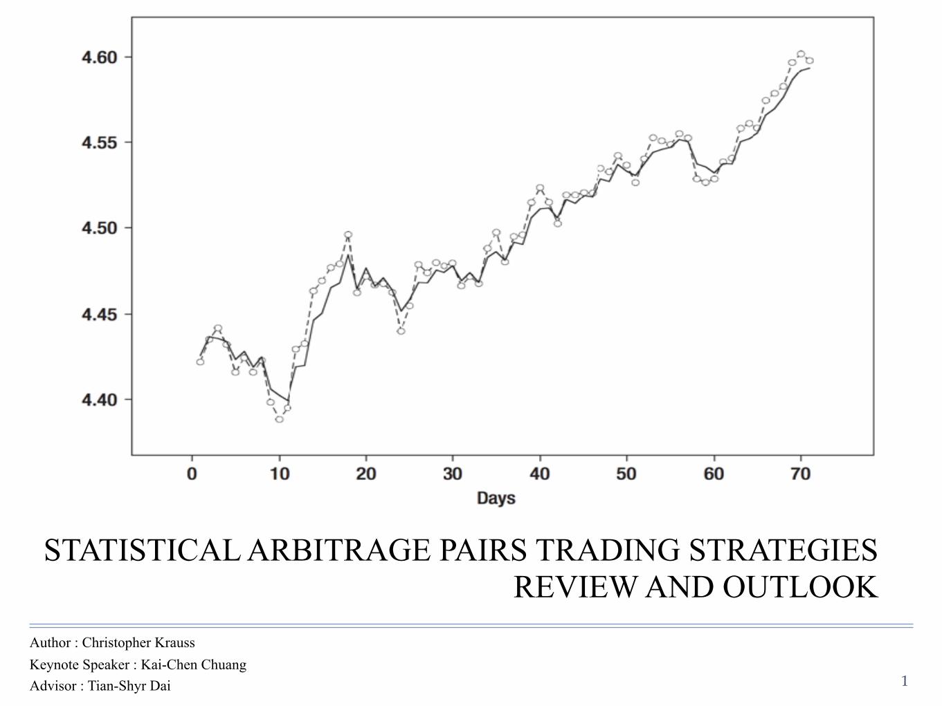
✤ According to Gatev et al. (2006), hereafter GGR, the concept of pairs trading is surprisingly simple and follows a two-step process.

✤ First, find two securities whose prices have moved together historically in a formation period.

✤ Second, monitor the spread between them in a subsequent trading period.

✤ If the prices diverge and the spread widens, short the winner and buy the loser.

✤ Two securities follow an equilibrium relationship, the spread will revert to its historical mean.

✤ The positions are reversed and a profit can be made.

✤ Quasi-multivariate frameworks : one security is traded against a weighted portfolio of comoving securities

✤ Multivariate frameworks : groups of stocks are traded against other groups of stocks.

3

Introduction

✤ The most cited paper in this domain is published by Gatev et al. (2006).

✤ Sample is tested on a large sample of U.S. equities, while rigorously controlling for data snooping bias.

✤ Yields annualized excess returns of up to 11% at low exposure to systematic sources of risk.

✤ profitability cannot be explained by previously documented reversal profits as in Jegadeesh (1990) and Lehmann (1990) or momentum profits as in Jegadeesh and Titman (1993).

✤ Despite these findings, academic research about pairs trading is still small compared to contrarian and momentum strategies.

4

Introduction

✤ Distance approach

✤ In the formation period, distance metrics are leveraged to identify comoving securities.

✤ In the trading period, simple nonparametric threshold rules are used to trigger trading signals.

✤ Cointegration approach

✤ In the formation period, cointegration tests are applied to identify comoving securities.

✤ The majority of trading signals based on GGR's threshold rule.

✤ The key benefit of these strategies is the econometrically more reliable equilibrium relationship of identified pairs.

5

Introduction

✤ Time-series approach

✤ All authors in this domain assume that a set of comoving securities has been established by prior analyses, so the formation period is generally ignored.

✤ The focus lies on the trading period and on generating optimized trading signals by different methods of time-series analysis.

✤ Stochastic control approach

✤ The formation period is ignored, too.

✤ Focus lies on identifying optimal portfolio holdings in the legs of a pairs trade compared to other assets.

✤ Stochastic control theory is used to determine value and optimal policy functions for this portfolio problem.

6

Introduction

✤ Other approaches

✤ Machine learning (ML) combined forecasts approach

✤ Copula approach

✤ Principal components analysis (PCA) approach.

7

Distance Approach 2.1 The Baseline Approach

✤ GGR’s study is performed on all liquid U.S. CRSP stocks from 1962 to 2002.

✤ A cumulative total return index is constructed for each stock and normalized to the first day of a 12-month formation period.

✤ With n stocks under consideration, the sum of Euclidean squared distance (SSD) for the price time series of n(n − 1)/2 possible combinations of pairs is calculated.

✤ The top 20 pairs with minimum historic SSD are considered in a subsequent six-month trading period.

✤ Trades are opened when the spread diverges by more than two historical standard deviations.

✤ Closed upon mean-reversion, at the end of the trading period, or upon delisting.

9


✤ Advantages of GGR’s approach

✤ Economic model-free

✤ Easy to implement

✤ Robust to data snooping

✤ Statistically significant risk-adjusted excess returns.

✤ Disadvantages of GGR’s approach

✤ The choice of Euclidean squared distance as selection metric is analytically suboptimal.

10


✤ It is trivial to see that an “ideal pair” in the sense of GGR with zero SSD has a spread of zero and thus produces no profits.


✤ Equation (2) shows that constraining for low SSD is the same as minimizing the sum of (i) spread variance and (ii) squared spread mean.

✤ Summand (ii) grows with spread mean drifting away from zero.

✤ Conversely, summand (i) grows with increasing deviations from this mean.

✤ Empirical result show decreasing spread volatility with decreasing SSD.

✤ Thus, GGR’s selection metric is prone to form pairs with low spread variance and limited profit potential.

12


✤ Mean-reversion. GGR interpret the pair’s price time series as cointegrated in sense of Bossaert(1988).

✤ However, the author develops a rigorous cointegration test based on canonical correlation analysis.

✤ Conversely, GGR perform no cointegration testing whatsoever (Galenko et al., 2012).

✤ The high correlation5 may well be spurious, since high correlation is not related to a cointegration relationship (Alexander, 2001).

✤ Spurious relationships based on an assumption of return parity are not mean-reverting.

✤ The potential lack of an equilibrium relationship leads to higher divergence risks and thus to potential losses.

13

Distance Approach 2.2 Expanding on the GGR Sample ✤ Do and Faff (2010, 2012) confirm declining profitability, mainly due to an increasing share of

nonconverging pairs.

✤ With the inclusion of trading costs, pairs trading according to GGR’s baseline methodology becomes largely unprofitable.

✤ They refined selection criteria to improve pairs identification.

✤ They only allow for matching securities within the 48 Fama–French industries.

✤ This restriction potentially leads to more meaningful pairs and fewer spurious correlations.

✤ There is also potential to miss out on interindustry opportunities.

✤ Pairs with a high number of zero-crossings in the formation period are favored.

✤ This algorithm are still slightly p

✤ rofitable, even after trading costs. 14

Distance Approach 2.3 From SSD to Pearson Correlation and Quasi-Multivariate Pairs Trading

✤ Chen et al. (2012) use the same data set and time frame as GGR, but opt for Pearson correlation on return level for identifying pairs.

✤ The authors construct an empirical metric to quantify return divergence dij between the returns of stock i and comover j

dij,t =β(ri,t −rf)−(rj,t −rf) t∈T (3)

Where β denotes the regression coefficient of stock i’s return realizations ri on its comover’s return realizations r j and r f is the risk-free rate.

✤ consider two cases for the comover return r j :

✤ In the univariate case, it is the return of the most highly correlated partner for stock i .

✤ In the quasi- multivariate case, it is the return of a comover portfolio, consisting of the equal-weighted returns of the 50 most highly correlated partners for stock i.

15


✤ All stocks are sorted in descending order based on their previous month’s return divergence and split into deciles.

✤ A dollar-neutral portfolio is constructed by longing decile 10 and shorting decile 1, and held for one month.

16


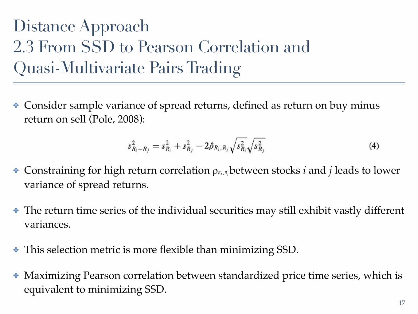
✤ Consider sample variance of spread returns, defined as return on buy minus return on sell (Pole, 2008):

✤ Constraining for high return correlation ρRi ,Rj between stocks i and j leads to lower variance of spread returns.

✤ The return time series of the individual securities may still exhibit vastly different variances.

✤ This selection metric is more flexible than minimizing SSD.

✤ Maximizing Pearson correlation between standardized price time series, which is equivalent to minimizing SSD.

17

Distance Approach 2.4 Explaining Pairs Trading Profitability

✤ GGR surmise that risk-adjusted excess returns of disjoint pairs portfolios are a compensation for a yet undiscovered latent risk factor.

✤ Andrade et al. (2005) replicate GGR’s approach in the Taiwanese stock market from 1994 to 2004.

✤ They confirm GGR’s findings out-of-sample.

✤ They find that the dominant factor behind spread divergence is uninformed buying and conclude that pairs trading profits are a compensation for liquidity provision to uninformed buyers.

18

✤ Papadakis and Wysocki (2007) analyze the impact of accounting events on pairs trading profitability between 1981 and 2006.

✤ They find that trades are often opened around earnings announcements and analyst forecasts.

✤ This research suggests that drift in stock prices after such events is a significant factor affecting pairs trading profitability.

✤ However, Do and Faff (2010) could not replicate these results on the extended GGR sample, casting doubt on the findings.

19


✤ Chen et al. (2012) confirm that pairs trading profitability is partly driven by delays in information diffusion across the two legs of a pair.

✤ Profitability is highest in poorer information environments.

✤ Jacobs and Weber (2013) confirm that pairs trading returns are linked to different diffusion speeds of common information across the two securities forming a pair.

20


Cointegration approach 3.1 Univariate Pairs Trading

3.1.1 Development of a Theoretical Framework

✤ Vidyamurthy (2004) provides the most cited work for cointegration-based pairs trading.

✤ Pairs are preselected based on statistical or fundamental similarity measures.

✤ Tradability is assessed, following an adapted version of the Engle–Granger cointegration test.

✤ Optimal entry/exit thresholds are designed with nonparametric methods.

21

3.1.2 A Large-Scale Empirical Application

✤ Rad et al. (2015) provide the first large-scale empirical application of the cointegration approach on U.S. CRSP data from 1962 until 2014, following GGR and Vidyamurthy (2004).

✤ The spread εi j,t between two stocks can be defined as with Pi and Pj denoting the I (1)-nonstationary price processes of stocks i and j .

✤ The cointegration coefficient γ is a nonzero real number, so that the spread εi j,t as linear combination of Pi and Pj is I(0)-stationary, hence mean-reverting.

✤ We say the two price processes are cointegrated.

✤ They test these stocks for cointegration with the Engle–Granger approach and only retain the top 20 stocks of the SSD ranking that are also cointegrated.

✤ Trading signals are generated with a variant of GGR’s threshold rule 22


✤ One USD is invested in the long leg of each pair and the dollar amount in the short leg is determined in line with the cointegration relationship in (5).

✤ Rad et al. (2015) find monthly excess returns of 0.83% prior to transaction costs for the cointegration approach—very similar to the 0.88% return of the distance method they run as benchmark.

✤ This lack of outperformance of the cointegration approach is possibly driven by the two-step pairs selection metric.

✤ Limiting cointegration to the subset of pairs with minimum SSD introduces a clear selection bias.

✤ Krauss recommend an end-to-end cointegration-based selection and trading algorithm.

23


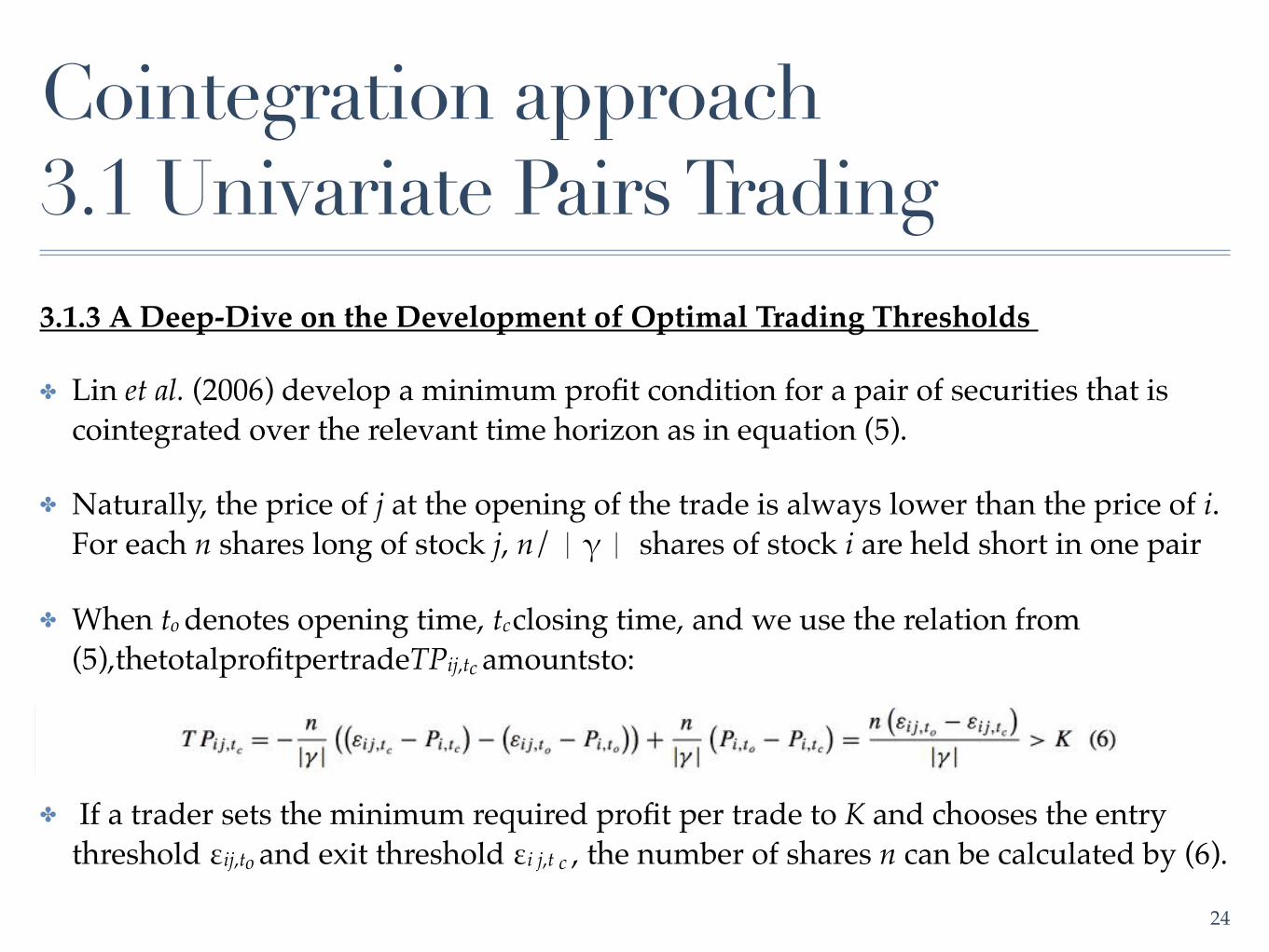
3.1.3 A Deep-Dive on the Development of Optimal Trading Thresholds

✤ Lin et al. (2006) develop a minimum profit condition for a pair of securities that is cointegrated over the relevant time horizon as in equation (5).

✤ Naturally, the price of j at the opening of the trade is always lower than the price of i. For each n shares long of stock j, n/｜γ｜ shares of stock i are held short in one pair

✤ When to denotes opening time, tc closing time, and we use the relation from (5),thetotalprofitpertradeTPij,tc amountsto:

✤ If a trader sets the minimum required profit per trade to K and chooses the entry threshold εij,to and exit threshold εi j,t c , the number of shares n can be calculated by (6).

24


The concept has several weaknesses.

1. The minimum profit per trade is set in absolute terms, so the profitability scaled by initial investment can become quite low,

2. The simulation study lacks diversity with only one cointegration model under review.

✤ It would be interesting to see how the trading rule performs in different cointegration settings, potentially allowing for the equilibrium relationship to shift or rupture.

3. The empirical application is limited to two stocks and a time frame of less than two years.

4. Vidyamurthy (2004) points out, total profit over a trading period is a function of the number of trades and the profit per trade.

✤ Optimizing profit per trade usually does not optimize total profit over the trading horizon.

25


3.1.4 A Review of Further Empirical Applications

✤ The first empirical applications are found in the domain of futures markets under the keyword “spread trading.”

✤ Girma and Paulson (1999) focus on the “crack spread,”

✤ The price difference between petroleum futures and futures on its refined end products.

✤ Different variants of this spread are stationary according to the augmented Dickey–Fuller (ADF) and the Phillips–Perron test.

✤ Trades are entered when the spread deviates a multiple k of its cross-sectional standard deviation from its cross-sectional moving average.

✤ Positions are closed when the spread returns to its own n-day moving average.

✤ After consideration of USD 100 transaction costs per full turn, average return still exceeds 15% p.a.8

26


✤ Simon (1999) successfully trades the crush spread.

✤ Emery and Liu (2002) analyze the spark spread.

✤ The gold–silver spread, Wahab and Cohn (1994) find trading to be unsuccessful.

✤ Hong and Susmel (2003) are the first authors to implement a rudimentary version of the cointegration approach to stocks.

✤ They choose 64 American Depositary Receipts (ADRs) and the corresponding shares in the local markets from 1991 to 2000.

✤ They choose 64 American Depositary Receipts (ADRs) and the corresponding shares in the local markets from 1991 to 2000.

✤ Only ADRs may be shorted due to potential short- selling restrictions in local markets. 27


✤ Dunis et al. (2010) test the univariate cointegration approach in a daily and a high-frequency setting on the constituents of the EuroStoxx 50 index.

✤ They restrict pairs formation to 10 industry groups and come up with 176 possible pairs.

✤ The spread for each pair is defined as

✤ where the time-varying parameter γt is estimated with the Kalman Filter.

✤ Next, the spreads of all pairs are calculated with equation (7), standardized, and then traded according to a simple standard deviation logic similar to GGR.

✤ They find that in-sample t-statistics of the ADF test as part of the Engle–Granger cointegration test and in-sample information ratios seem to have certain predictive power for out-of-sample information ratios.

28


✤ Caldeira and Moura (2013) apply the univariate cointegration approach to the 50 most liquid stocks of the Brazilian stock index IBovespa.

✤ They use the Engle–Granger approach as well as the Johansen method at the 5% significance level to test for cointegration relationships and find 90 cointegrated pairs.

✤ These pairs are ranked according to the in-sample Sharpe ratio.

✤ The top 20 pairs are selected for a four- month trading period.

✤ Positions are opened and closed based on a modified standard deviation rule similar to GGR.

✤ Caldeira and Moura (2013) show statistically significant excess returns after consideration of transaction costs and robust to data snooping based on the reality check of White (2000) and the SPA test of Hansen (2005).

✤ The Engle–Granger and the Johansen tests are not statistically independent when used on the same data set.

29


✤ Gutierrez and Tse (2011) provide an appealing conceptual framework that is applied to a set of three cointegrated stocks.

✤ For each pair, the Granger-leaders and Granger-followers are identified.

✤ The majority of profitability stems from the Granger-follower, whereas the Granger-leader barely contributes.

✤ Li et al. (2014) show that cointegration-based pairs trading is profitable in the Chinese AH-share markets.

✤ Afawubo (2015) analyze the cointegration approach and the distance approach for the S&P 500 constituents and under varying parameterizations.

✤ After consideration of risk loadings and transaction costs, they find that the cointegration approach significantly outperforms the distance method.

30


✤ 3.2.1 Passive Index Tracking and Enhanced Indexation Strategies

✤ Dunis and Ho (2005) use cointegration relationships to construct index tracking portfolios for the EuroStoxx 50 index.

✤ Dunis and Ho (2005) take different subsets (5, 10, 15, or 20 stocks) of the index constituents and estimate the joint cointegration vector for these constituents and their index.

✤ They measure the tracking error return of this basket versus the index for different rebalancing frequencies.

✤ They find that the tracking baskets produce a positive tracking error, resulting in an outperformance versus the benchmark.

✤ They develop an advanced indexation strategy.

✤ A synthetic “plus” benchmark is constructed by adding uniformly distributed returns of z percent p.a. to the daily returns of the EuroStoxx 50.

✤ Long the “plus” benchmark and short the “minus” benchmark allows for a market neutral investment strategy with potential “double alpha.”

31

Cointegration approach 3.2 Multivariate Cointegration Approach

3.2.2 Active Statistical Arbitrage Strategies

✤ Galenko et al. (2012) develop an active statistical arbitrage strategy based on a multivariate cointegration framework.

✤ Whereas correlation reflects short-term linear dependence in returns, cointegration models long-term dependencies in prices (Alexander, 2001).

✤ Excess returns are not tested for statistical significance.

32


3.3 Adjacent Developments

✤ Burgess (1999) develops a holistic statistical arbitrage framework relying on a combination of cointegration and emerging techniques such as neural networks and genetic algorithms.

✤ Burgess (2003) presents a simplified variant of this approach, solely relying on cointegration testing.

✤ Peters et al. (2011), Gatarek et al. (2011), and Gatarek et al. (2014) use Bayesian procedures for cointegration testing

33


✤ Gatev et al. (2006) already perform a set of robustness checks.

✤ They address the issue of bid-ask bounce (Jegadeesh, 1990).

✤ The price of the short leg is more likely to be an ask quote and the price of the long leg a bid quote.

✤ For convergence, the opposite holds, so results may systematically be biased upwards.

✤ GGR introduce a one- day-waiting rule after each trading signal, reducing average excess returns by 0.54% per month for the top 20 pairs.

34

Pairs Trading in the Light of Market Frictions

✤ GGR provide a rough estimation for transaction costs.

✤ GGR estimate transaction costs of 3.24% for two round-trips compared to profits of 5.49%, leading to statistically and economically significant excess returns of 2.25% after transaction costs.

✤ They also consider explicit short-selling costs.

✤ These explicit costs in the form of specials have a minimal effect on large stocks

✤ Also, they simulate implicit short-selling costs in the form of recalls, leading to a slight reduction in pairs trading profitability.

35


✤ Do and Faff (2012) analyze the impact of trading costs on pairs trading profitability. In particular, they account for commissions, market impact, and short-selling fees.

✤ The authors consider time-varying commissions, with average one-way costs of 0.34% over the full sample period.

✤ Market impact or slippage can be defined as difference between expected price and price actually paid.

✤ Do and Faff (2012) perform an estimation by monitoring the spread at divergence and for the two subsequent days.

✤ It narrows by 0.26% on the first day and by an additional 0.12% on the second day after divergence.

✤ If an investor faces slower execution, slippage may be even higher.

✤ A short-selling fee of 1% p.a., payable over the duration of each trade, is applied.

✤ Considering all three cost dimensions, pairs trading in the sense of GGR becomes unprofitable.

36


Date post:	19-Mar-2022
Category:	Documents
Upload:	others
View:	13 times
Download:	0 times

STATISTICAL ARBITRAGE PAIRS TRADING STRATEGIES REVIEW …

Documents