STATISTICAL DATA ANALYSIS IN...

Statistical data analysis in Excel

STATISTICAL DATA STATISTICAL DATA

ANALYSIS IN EXCELANALYSIS IN EXCEL

14-06-2010

Dr. Dr. PetrPetr NazarovNazarov

[email protected]@crp--sante.lusante.lu

Part 2Part 2

Practical AspectsPractical Aspects

Microarray CenterMicroarray Center

Statistical data analysis in Excel 2

Hypotheses (theoretical)

Unpaired t-test

Paired t-test

ANOVA

Linear regression

Multiple comparison

Empirical confidence interval calculation

Goodness of fit and inependence (optional)

OUTLINE

http://edu.sablab.net/datahttp://edu.sablab.net/data


HYPOTHESESHYPOTHESES

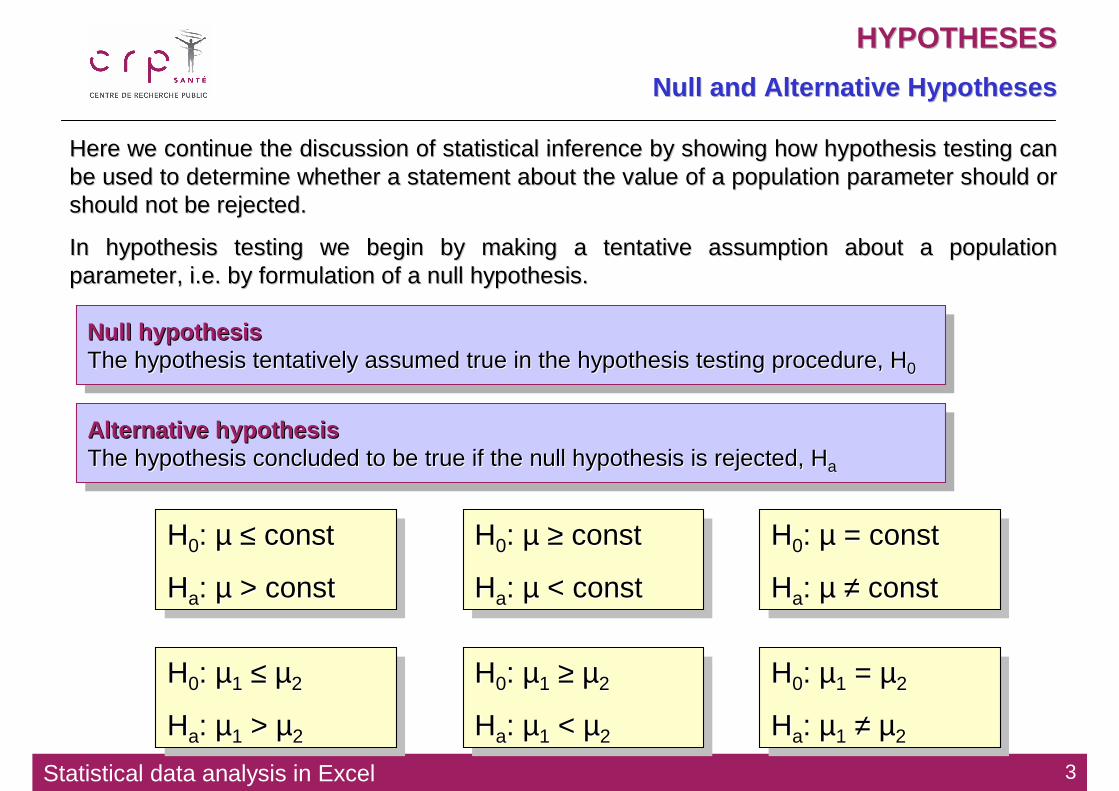
Null and Alternative HypothesesNull and Alternative Hypotheses

Null hypothesisThe hypothesis tentatively assumed true in the hypothesis testing procedure, H0

Null hypothesisNull hypothesisThe hypothesis tentatively assumed true in the hypothesis testinThe hypothesis tentatively assumed true in the hypothesis testing procedure, g procedure, HH00

Alternative hypothesisThe hypothesis concluded to be true if the null hypothesis is rejected, Ha

Alternative hypothesisAlternative hypothesisThe hypothesis concluded to be true if the null hypothesis is reThe hypothesis concluded to be true if the null hypothesis is rejected, jected, HHaa

Here we continue the discussion of statistical inference by showHere we continue the discussion of statistical inference by showing how hypothesis testing can ing how hypothesis testing can be used to determine whether a statement about the value of a pobe used to determine whether a statement about the value of a population parameter should or pulation parameter should or should not be rejected.should not be rejected.

In hypothesis testing we begin by making a tentative assumption In hypothesis testing we begin by making a tentative assumption about a population about a population parameter, i.e. by formulation of a null hypothesis.parameter, i.e. by formulation of a null hypothesis.

H0: µ ≤ const

Ha: µ > const

HH00: : µµ ≤≤ constconst

HHaa: : µµ > const> const

H0: µ ≥ const

Ha: µ < const

HH00: : µµ ≥≥ constconst

HHaa: : µµ < const< const

H0: µ = const

Ha: µ ≠ const

HH00: : µµ = const= const

HHaa: : µµ ≠≠ constconst

H0: µ1 ≤ µ2

Ha: µ1 > µ2

HH00: : µµ11 ≤≤ µµ22

HHaa: : µµ11 > > µµ22

H0: µ1 ≥ µ2

Ha: µ1 < µ2

HH00: : µµ11 ≥≥ µµ22

HHaa: : µµ11 < < µµ22

H0: µ1 = µ2

Ha: µ1 ≠ µ2

HH00: : µµ11 = = µµ22

HHaa: : µµ11 ≠≠ µµ22



Type I ErrorType I Error

Type I errorThe error of rejecting H0 when it is true.

Type I errorType I errorThe error of rejecting The error of rejecting HH00 when it is true.when it is true.

Type II errorThe error of accepting H0 when it is false.

Type II errorType II errorThe error of accepting The error of accepting HH00 when it is false.when it is false.

False False PPositive,ositive,αααααααα errorerror

poor specificitypoor specificity

False False NNegative,egative,ββββββββ errorerror

poor sensitivitypoor sensitivityLevel of significanceThe probability of making a Type I error when the null hypothesis is true as an equality

Level of significanceLevel of significanceThe probability of making a Type I error when The probability of making a Type I error when the null hypothesis is true as an equalitythe null hypothesis is true as an equality



OneOne--tailed Testtailed Test

Test statisticA statistic whose value helps determine whether a null hypothesis can be rejected

Test statisticTest statisticA statistic whose value helps determine whether A statistic whose value helps determine whether a null hypothesis can be rejecteda null hypothesis can be rejected n

mz

σµ0−

=

H0: µ ≥ 3

Ha: µ < 3

HH00: : µµ ≥≥ 33

HHaa: : µµ < 3< 3

Step 1. Introduce the test statisticsStep 1. Introduce the test statistics

Assume that we have obtained experimentally m=2.92. Is it Assume that we have obtained experimentally m=2.92. Is it significant?significant?



OneOne--tailed Testtailed Test

Step 2. Calculate pStep 2. Calculate p --value and compare it with value and compare it with αααααααα

p-valueA probability, computed using the test statistic, that measures the support (or lack of support) provided by the sample for the null hypothesis. It is a probability of making error of type I

pp--valuevalueA probability, computed using the test statistic, that measures A probability, computed using the test statistic, that measures the support (or lack of the support (or lack of support) provided by the sample for the null hypothesis. It is asupport) provided by the sample for the null hypothesis. It is a probability of making probability of making error of type I error of type I

p > αααα ⇒⇒⇒⇒ H0p < αααα ⇒⇒⇒⇒ Ha

p > p > αααααααα ⇒⇒⇒⇒⇒⇒⇒⇒ HH00

p < p < αααααααα ⇒⇒⇒⇒⇒⇒⇒⇒ HHaa



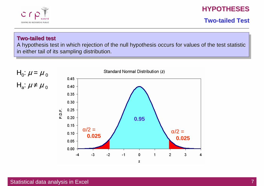
TwoTwo --tailed Testtailed Test

Two-tailed testA hypothesis test in which rejection of the null hypothesis occurs for values of the test statistic in either tail of its sampling distribution.

TwoTwo --tailed testtailed testA hypothesis test in which rejection of the null hypothesis occuA hypothesis test in which rejection of the null hypothesis occurs for values of the test statistic rs for values of the test statistic in either tail of its sampling distribution. in either tail of its sampling distribution.

HH00: : µµ = = µµ 00

HHaa: : µµ ≠≠ µµ 00

0.950.95

0.0250.025 0.0250.025

αα/2 = /2 = αα/2 = /2 =



σσσσσσσσ is Unknownis Unknown

if σσσσ in unknown:σσσσ → sz → t

if if σσσσσσσσ in unknown:in unknown:σσσσσσσσ →→ sszz →→ tt

Lower Tail Test Upper Tail Test Two-Tailed Test

Hypotheses 00 : µµ ≥H

0: µµ <aH

00 : µµ ≤H

0: µµ >aH

00 : µµ =H

0: µµ ≠aH

Test Statistic

ns

mt 0µ−=

ns

mt 0µ−=

ns

mt 0µ−=

Rejection Rule:

p-Value Approach

Reject H0 if

p-value ≤ α

Reject H0 if

p-value ≤ α

Reject H0 if

p-value ≤ α

Rejection Rule:

Critical Value Approach

Reject H0 if

t ≤ –tα

Reject H0 if

t ≥ tα

Reject H0 if

2αtt −≤ or if

2αtt ≥


HYPOTHESIS TESTING FOR THE MEANHYPOTHESIS TESTING FOR THE MEAN

One Tail Test vs. Two Tail TestOne Tail Test vs. Two Tail Test

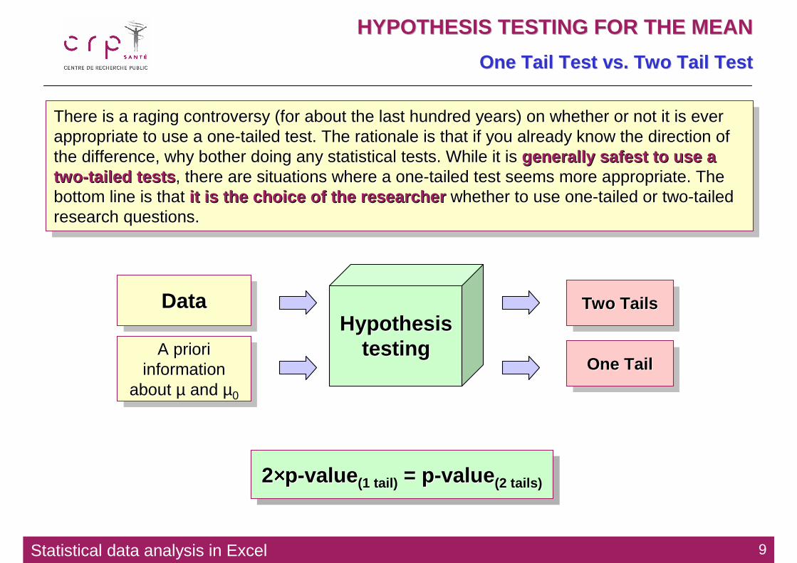
There is a raging controversy (for about the last hundred years) on whether or not it is ever appropriate to use a one-tailed test. The rationale is that if you already know the direction of the difference, why bother doing any statistical tests. While it is generally safest to use a two-tailed tests , there are situations where a one-tailed test seems more appropriate. The bottom line is that it is the choice of the researcher whether to use one-tailed or two-tailed research questions.

There is a raging controversy (for about the last hundred years)There is a raging controversy (for about the last hundred years) on whether or not it is ever on whether or not it is ever appropriate to use a oneappropriate to use a one--tailed test. The rationale is that if you already know the directailed test. The rationale is that if you already know the direction of tion of the difference, why bother doing any statistical tests. While itthe difference, why bother doing any statistical tests. While it is is generally safest to use a generally safest to use a twotwo --tailed teststailed tests , there are situations where a one, there are situations where a one--tailed test seems more appropriate. The tailed test seems more appropriate. The bottom line is that bottom line is that it is the choice of the researcherit is the choice of the researcher whether to use onewhether to use one--tailed or twotailed or two--tailed tailed research questions.research questions.

HypothesisHypothesistestingtesting

Data Data Data

A priori information

about µ and µ0

A priori A priori information information

about about µµ and and µµ00

Two TailsTwo TailsTwo Tails

One TailOne TailOne Tail

2××××p-value (1 tail) = p-value (2 tails)22××××××××pp--valuevalue (1 tail)(1 tail) = p= p--valuevalue (2 tails)(2 tails)


Unpaired tUnpaired t --testtest


UNPAIRED tUNPAIRED t --TESTTEST

Independent SamplesIndependent Samples

Independent samples Samples selected from two populations in such a way that the elements making up one sample are chosen independently of the elements making up the other sample.

Independent samples Independent samples Samples selected from two populations in such a way that the eleSamples selected from two populations in such a way that the elements making up one ments making up one sample are chosen independently of the elements making up the otsample are chosen independently of the elements making up the other sample.her sample.

WeightWeightWeight

HeightHeightHeight

SmokingSmokingSmoking



ExampleExample

mice.xlsmice.xls

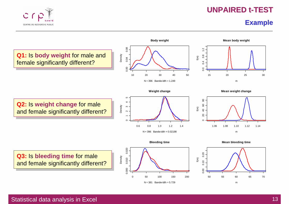
Q1: Is body weight for male and female significantly different?


Q2: Is weight change for male and female significantly different?


f m

1020

3040

Final body weights (g)

10 20 30 40 50

0.00

0.04

N = 394 Bandw idth = 1.499

Den

sity

Body weight distributions

f m

0.9

1.0

1.1

1.2

1.3

Weights change (g)

0.8 0.9 1.0 1.1 1.2 1.3 1.4

01

23

45

N = 394 Bandw idth = 0.02154

Den

sity

Distributions of weight change

f m

2060

100

Bleeding time (g)

0 50 100 150 200

0.00

00.

010

0.02

0

N = 381 Bandw idth = 5.729

Den

sity

Distributions of bleeding times

Q3: Is bleeding time for male and female significantly different?




ExampleExample

10 20 30 40 50

0.00

0.04

0.08

N = 396 Bandw idth = 1.249

Den

sity

Body weight

15 20 25 30

0.0

0.4

0.8

1.2

Mean body weight

m

f(m

)

0.6 0.8 1.0 1.2 1.40

12

34

5

N = 396 Bandw idth = 0.02198

Den

sity

Weight change

1.06 1.08 1.10 1.12 1.14

020

4060

80

Mean weight change

m

f(m

)

0 50 100 150 200

0.00

00.

010

0.02

0

N = 381 Bandw idth = 5.729

Den

sity

Bleeding time

50 55 60 65 70

0.00

0.10

0.20

Mean bleeding time

m

f(m

)









Practical TaskPractical Task

Using the tUsing the t--test define which parameter in the table is test define which parameter in the table is sexsex--dependentdependent

= TTEST (array1, array2, 2, 3)

mice.xlsmice.xls

parameter pval female maleStarting age 0.165799 65.90 66.52Ending age 0.223033 113.91 114.61Starting weight 5.48E-34 18.91 23.86Ending weight 8.98E-38 20.62 26.78Weight change 0.001405 1.09 1.12Bleeding time 0.248716 62.34 59.67Ionized Ca in blood 0.271336 1.23 1.24Blood pH 0.009593 7.21 7.19Bone mineral density 2.41E-05 0.05 0.05Lean tissues weight 4.66E-33 15.32 19.21Fat weight 2.28E-21 4.85 7.30


Paired tPaired t --testtest


Before treatmentBefore treatment

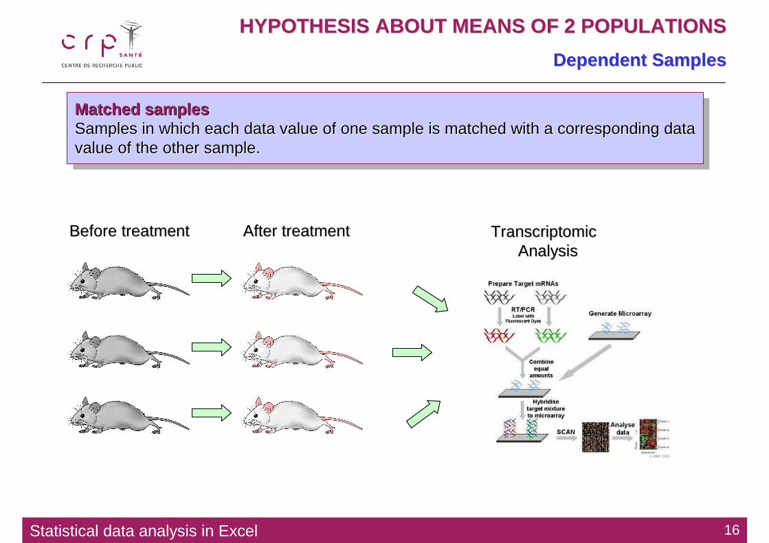
HYPOTHESIS ABOUT MEANS OF 2 POPULATIONSHYPOTHESIS ABOUT MEANS OF 2 POPULATIONS

Dependent SamplesDependent Samples

Matched samples Samples in which each data value of one sample is matched with a corresponding data value of the other sample.

Matched samples Matched samples Samples in which each data value of one sample is matched with aSamples in which each data value of one sample is matched with a corresponding data corresponding data value of the other sample.value of the other sample.

TranscriptomicTranscriptomicAnalysisAnalysis

After treatmentAfter treatment


HYPOTHESIS ABOUT MEANS OF 2 POPULATIONSHYPOTHESIS ABOUT MEANS OF 2 POPULATIONS

Paired tPaired t --test: Tasktest: Task

Unpaired test

• = TTEST (array1, array2, 2, 3)

Paired test

• = TTEST (array1, array2, 2, 1)

bloodpressure.xlsbloodpressure.xls

Subject BP before BP after1 122 1272 126 1283 132 1404 120 1195 142 1456 130 1307 142 1488 137 1359 128 129

10 132 13711 128 12812 129 133

Systolic blood pressure (mmHg)Systolic blood pressure (mmHg)

The systolic blood pressures of n=12 women between the The systolic blood pressures of n=12 women between the ages of 20 and 35 were measured before and after usage ages of 20 and 35 were measured before and after usage of a newly developed oral contraceptive.of a newly developed oral contraceptive.

Q: Does the treatment affect the systolic blood pressure?Q: Does the treatment affect the systolic blood pressure?

Test p-valueunpaired 0.414662paired 0.014506


ANOVAANOVA


INTRODUCTION TO ANOVA

Why ANOVA?

Means for more than 2 populationsWe have measurements for 5 conditions. Are the means for these conditions equal?

Means for more than 2 populationsWe have measurements for 5 conditions. Are the means for these conditions equal?

Validation of the effectsWe assume that we have several factors affecting our data. Which factors are more significant? Which can be neglected?

Validation of the effectsWe assume that we have several factors affecting our data. Which factors are more significant? Which can be neglected?

If we would use If we would use pairwisepairwise comparisons, comparisons, what will be the probability of getting error?what will be the probability of getting error?

Number of comparisons:Number of comparisons: 10!3!2

!552 ==C

Probability of an errorProbability of an error: 1: 1––(0.95)(0.95)10 10 = = 0.40.4

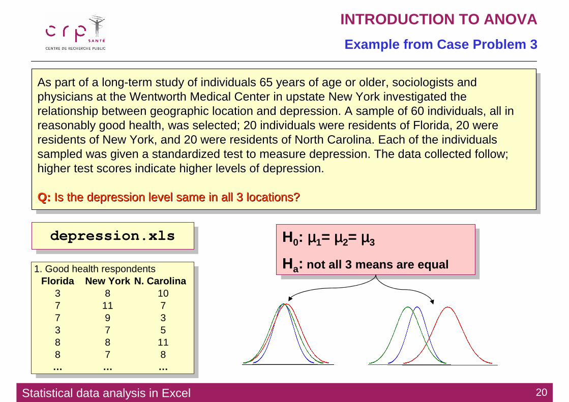
http://easylink.playstream.com/affymetrix/ambsymposium/partek_08.wvx



Example from Case Problem 3

As part of a long-term study of individuals 65 years of age or older, sociologists and physicians at the Wentworth Medical Center in upstate New York investigated the relationship between geographic location and depression. A sample of 60 individuals, all in reasonably good health, was selected; 20 individuals were residents of Florida, 20 were residents of New York, and 20 were residents of North Carolina. Each of the individuals sampled was given a standardized test to measure depression. The data collected follow; higher test scores indicate higher levels of depression.

Q: Is the depression level same in all 3 locations?

As part of a longAs part of a long--term study of individuals 65 years of age or older, sociologiststerm study of individuals 65 years of age or older, sociologists and and physicians at the Wentworth Medical Center in upstate New York iphysicians at the Wentworth Medical Center in upstate New York investigated the nvestigated the relationship between geographic location and depression. A samplrelationship between geographic location and depression. A sample of 60 individuals, all in e of 60 individuals, all in reasonably good health, was selected; 20 individuals were residereasonably good health, was selected; 20 individuals were residents of Florida, 20 were nts of Florida, 20 were residents of New York, and 20 were residents of North Carolina. residents of New York, and 20 were residents of North Carolina. Each of the individuals Each of the individuals sampled was given a standardized test to measure depression. Thesampled was given a standardized test to measure depression. The data collected follow; data collected follow; higher test scores indicate higher levels of depression. higher test scores indicate higher levels of depression.

Q: Q: Is the depression level same in all 3 locations?Is the depression level same in all 3 locations?

H0: µµµµ1= µµµµ2= µµµµ3

Ha: not all 3 means are equal



depression.xlsdepression.xls

1. Good health respondentsFlorida New York N. Carolina

3 8 107 11 77 9 33 7 58 8 118 7 8… … …



Meaning





0

2

4

6

8

10

12

14F

L

FL

FL

FL

FL

FL

FL

NY

NY

NY

NY

NY

NY

NY

NC

NC

NC

NC

NC

NC

Measures

Dep

ress

ion

leve

l

mm11

mm22

mm33


SINGLE-FACTOR ANOVA

Example

0

2

4

6

8

10

12

14

FL

FL

FL

FL

FL

FL

FL

NY

NY

NY

NY

NY

NY

NY

NC

NC

NC

NC

NC

NC

Measures

Dep

ress

ion

leve

l

mm11

mm22

mm33

SSESSTRSST +=


SINGLE-FACTOR ANOVA

Example

ANOVA table A table used to summarize the analysis of variance computations and results. It contains columns showing the source of variation, the sum of squares, the degrees of freedom, the mean square, and the F value(s).

ANOVA table A table used to summarize the analysis of variance computations and results. It contains columns showing the source of variation, the sum of squares, the degrees of freedom, the mean square, and the F value(s).

In Excel use:

Tools → Data Analysis → ANOVA Single Factor

LetLet’’s perform for dataset 1: s perform for dataset 1: ““good healthgood health””


ANOVASource of Variation SS df MS F P-value F crit

Between Groups 78.53333 2 39.26667 6.773188 0.002296 3.158843Within Groups 330.45 57 5.797368

Total 408.9833 59

SSTRSSTR

SSESSE


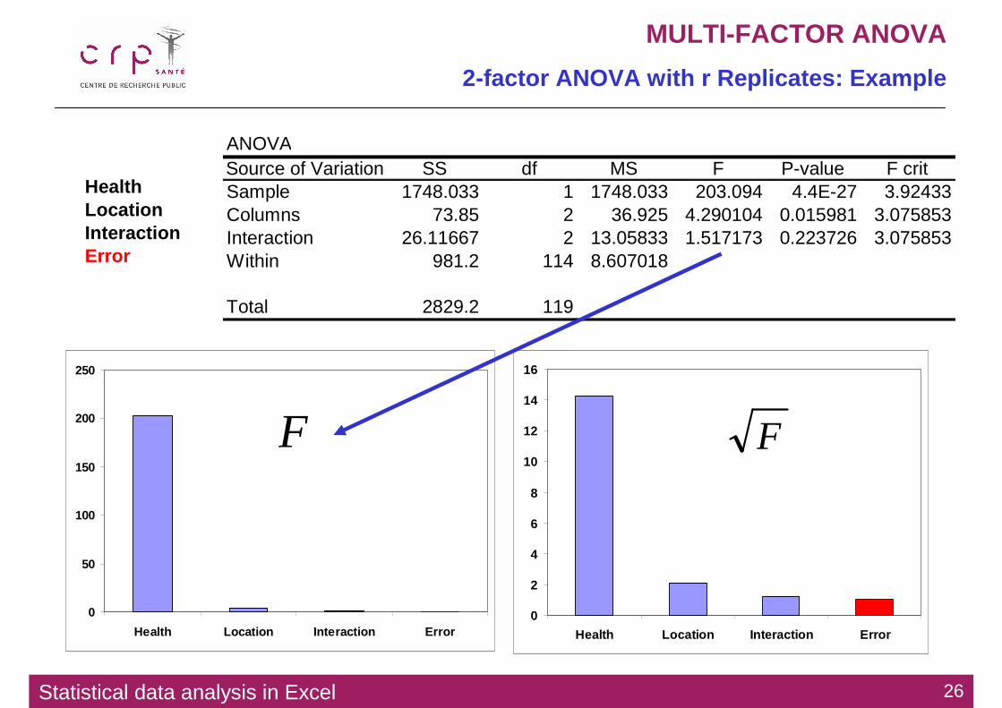
MULTI-FACTOR ANOVA

Factors and Treatments

Factor Another word for the independent variable of interest.

Factor Another word for the independent variable of interest.

Treatments Different levels of a factor.

Treatments Different levels of a factor.

depression.xlsdepression.xlsFactor 1:Factor 1: Health Health

good healthgood health

bad health bad health

Factor 2:Factor 2: LocationLocation

FloridaFlorida

New YorkNew York

North CarolinaNorth Carolina

Factorial experiment An experimental design that allows statistical conclusions about two or more factors.

Factorial experiment An experimental design that allows statistical conclusions about two or more factors.

Depression = µ + Health + Location + Health×Location + εDepression = µ + Health + Location + Health×Location + ε

Interaction The effect produced when the levels of one factor interact with the levels of another factor in influencing the response variable.

Interaction The effect produced when the levels of one factor interact with the levels of another factor in influencing the response variable.


MULTI-FACTOR ANOVA

2-factor ANOVA with r Replicates: Example


1.1. Reorder the data into format understandable for Excel Reorder the data into format understandable for Excel

Factor 1:Factor 1: Health Health

Factor 2:Factor 2: LocationLocation

Florida New York North CarolinaGood health 3 8 10

7 11 77 9 33 7 5… … …

7 7 83 8 11

bad health 13 14 1012 9 1217 15 1517 12 18… … …

11 13 1317 11 11

2.2. Use Tools Use Tools →→ Data Analysis Data Analysis →→ANOVA: TwoANOVA: Two--factor with replicatesfactor with replicates


0

2

4

6

8

10

12

14

16

Health Location Interaction Error

MULTI-FACTOR ANOVA

2-factor ANOVA with r Replicates: Example

HealthLocationInteractionError

F

ANOVASource of Variation SS df MS F P-value F critSample 1748.033 1 1748.033 203.094 4.4E-27 3.92433Columns 73.85 2 36.925 4.290104 0.015981 3.075853Interaction 26.11667 2 13.05833 1.517173 0.223726 3.075853Within 981.2 114 8.607018

Total 2829.2 119

0

50

100

150

200

250

Health Location Interaction Error

F


Linear RegressionLinear Regression


LINEAR REGRESSION

Experiments

Dependent variable The variable that is being predicted or explained. It is denoted by y.

Dependent variable The variable that is being predicted or explained. It is denoted by y.

Independent variable The variable that is doing the predicting or explaining. It is denoted by x.

Independent variable The variable that is doing the predicting or explaining. It is denoted by x.

Temperature Cell Number20 8321 13922 9923 14324 16425 23326 19827 26128 23529 26430 24331 33932 33133 34634 35035 36836 36037 39738 36139 35840 381

0

50

100

150

200

250

300

350

400

450

15 25 35 45

Temperature

Num

ber o

f cel

ls

xx

yy Cells are grown under different temperature conditions from 20°to 40°. A researched would like to find a dependency between T and cell number.

Cells are grown under different Cells are grown under different temperature conditions from 20temperature conditions from 20°°to 40to 40°°. A researched would like to . A researched would like to find a dependency between T and find a dependency between T and cell number. cell number.


LINEAR REGRESSION

Experiments

Simple linear regression Regression analysis involving one independent variable and one dependent variable in which the relationship between the variables is approximated by a straight line.

Simple linear regression Regression analysis involving one independent variable and one dependent variable in which the relationship between the variables is approximated by a straight line.

Building a Building a regressionregression means finding and tuning the means finding and tuning the modelmodel to explain the behaviour of the to explain the behaviour of the datadata

0

50

100

150

200

250

300

350

400

450

15 25 35 45

Temperature

Num

ber o

f cel

ls


LINEAR REGRESSION

Experiments

εββ ++= 01)( xxy

Model for a simple linear regression:Model for a simple linear regression:

0

50

100

150

200

250

300

350

400

450

15 25 35 45

Temperature

Num

ber o

f cel

ls

Regression model The equation describing how y is related to x and an error term; in simple linear regression, the regression model is y = ββββ0 + ββββ1x + εεεε

Regression model The equation describing how y is related to x and an error term; in simple linear regression, the regression model is y = ββββ0 + ββββ1x + εεεε

Regression equation The equation that describes how the mean or expected value of the dependent variable is related to the independent variable; in simple linear regression, E(y) =ββββ0 + ββββ1x

Regression equation The equation that describes how the mean or expected value of the dependent variable is related to the independent variable; in simple linear regression, E(y) =ββββ0 + ββββ1x


LINEAR REGRESSION

Regression Model and Regression Line

εββ ++= 01)( xxy


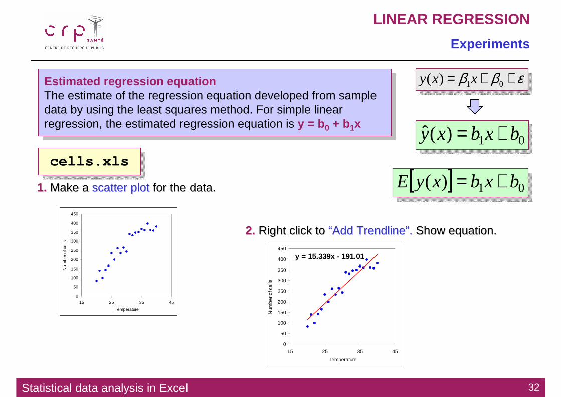
LINEAR REGRESSION

Experiments

Estimated regression equation The estimate of the regression equation developed from sample data by using the least squares method. For simple linear regression, the estimated regression equation is y = b0 + b1x

Estimated regression equation The estimate of the regression equation developed from sample data by using the least squares method. For simple linear regression, the estimated regression equation is y = b0 + b1x

cells.xlscells.xls

1.1. Make aMake a scatter plot scatter plot for the data.for the data.

0

50

100

150

200

250

300

350

400

450

15 25 35 45

Temperature

Num

ber o

f cel

ls

2.2. Right click toRight click to ““Add Add TrendlineTrendline””. . Show equation.Show equation.

y = 15.339x - 191.01

0

50

100

150

200

250

300

350

400

450

15 25 35 45

Temperature

Num

ber o

f cel

ls

εββ ++= 01)( xxy

01)(ˆ bxbxy +=

[ ] 01)( bxbxyE +=


LINEAR REGRESSION

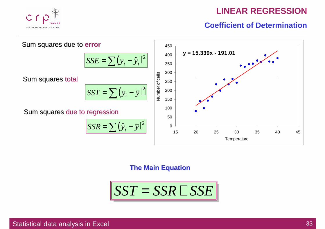
Coefficient of Determination

( )2ˆ∑ −= ii yySSE

Sum squares due to Sum squares due to errorerrory = 15.339x - 191.01

0

50

100

150

200

250

300

350

400

450

15 20 25 30 35 40 45

Temperature

Num

ber o

f cel

ls

( )2∑ −= yySST i

Sum squares Sum squares totaltotal

( )2ˆ∑ −= yySSR i

Sum squares Sum squares due to regressiondue to regression

SSESSRSST +=

The Main EquationThe Main Equation


LINEAR REGRESSION

Coefficient of Determination

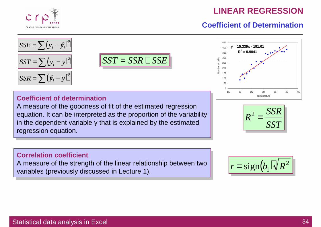
Coefficient of determination A measure of the goodness of fit of the estimated regression equation. It can be interpreted as the proportion of the variability in the dependent variable y that is explained by the estimated regression equation.

Coefficient of determination A measure of the goodness of fit of the estimated regression equation. It can be interpreted as the proportion of the variability in the dependent variable y that is explained by the estimated regression equation.

( )2€∑ −= ii yySSE

( )2∑ −= yySST i

( )2€∑ −= yySSR i

SSESSRSST +=

SST

SSRR =2

y = 15.339x - 191.01R2 = 0.9041

0

50

100

150

200

250

300

350

400

450

15 20 25 30 35 40 45

Temperature

Num

ber o

f cel

ls

Correlation coefficient A measure of the strength of the linear relationship between twovariables (previously discussed in Lecture 1).

Correlation coefficient A measure of the strength of the linear relationship between twovariables (previously discussed in Lecture 1).

( ) 21sign Rbr =


LINEAR REGRESSION

Assumptions

εββ ++= 01)( xxyAssumptions for Simple Linear Regression1. The error term εεεε is a random variable with 0 mean, i.e. E[ε]=02. The variance of εεεε, denoted by σσσσ 2, is the same for all values of x3. The values of εεεε are independent3. The term εεεε is a normally distributed variable

Assumptions for Simple Linear Regression1. The error term εεεε is a random variable with 0 mean, i.e. E[ε]=02. The variance of εεεε, denoted by σσσσ 2, is the same for all values of x3. The values of εεεε are independent3. The term εεεε is a normally distributed variable


LINEAR REGRESSION

ANOVA and Regression: Testing for Significance

0

2

4

6

8

10

12

14

FL

FL

FL

FL

FL

FL

FL

NY

NY

NY

NY

NY

NY

NY

NC

NC

NC

NC

NC

NC

Measures

Dep

ress

ion

leve

l

mm11

mm22

mm33

SSESSTRSST +=

0

50

100

150

200

250

300

350

400

450

15 20 25 30 35 40 45

Temperature

Num

ber o

f cel

ls

SSESSRSST +=

H0: ββββ1 = 0 insignificant

Ha: ββββ1 ≠≠≠≠ 0

H0: ββββ1 = 0 insignificant

Ha: ββββ1 ≠≠≠≠ 0


REGRESSION ANALYSIS

Example

cells.xlscells.xls In Excel use the function:

= INTERCEPT(y,x)

= SLOPE(y,x)

1.1. Calculate manually Calculate manually bb11 and and bb00

Intercept b0= -191.008119Slope b1= 15.3385723

Tools Tools →→ Data Analysis Data Analysis →→ RegressionRegression2.2. LetLet’’s do it automaticallys do it automatically

SUMMARY OUTPUT

Regression StatisticsMultiple R 0.950842308R Square 0.904101095Adjusted R Square 0.899053784Standard Error 31.80180903Observations 21

ANOVAdf SS MS F Significance F

Regression 1 181159.2853 181159.3 179.1253 4.01609E-11Residual 19 19215.7461 1011.355Total 20 200375.0314

Coefficients Standard Error t Stat P-value Lower 95% Upper 95% Lower 95.0% Upper 95.0%Intercept -191.0081194 35.07510626 -5.445689 2.97E-05 -264.4211603 -117.5950784 -264.4211603 -117.5950784X Variable 1 15.33857226 1.146057646 13.38377 4.02E-11 12.93984605 17.73729848 12.93984605 17.73729848


REGRESSION ANALYSIS

Confidence and Prediction

Confidence interval The interval estimate of the mean value of y for a given value of x.

Confidence interval The interval estimate of the mean value of y for a given value of x.

Prediction interval The interval estimate of an individual value of y for a given value of x.

Prediction interval The interval estimate of an individual value of y for a given value of x.


REGRESSION ANALYSIS

Residuals


Correction for Multiple ComparisonCorrection for Multiple Comparison

all_data.xlsall_data.xlsPlease download the data from Please download the data from edu.sablab.net/data/xlsedu.sablab.net/data/xls


MULTIPLE EXPERIMENTS

Correct Results and Errors

False False PPositive,ositive,αααααααα errorerror

False False NNegative,egative,ββββββββ errorerror

Probability of an error in a multiple test: Probability of an error in a multiple test:

11––(0.95)(0.95)number of comparisonsnumber of comparisons



False Discovery Rate

False discovery rate (FDR)FDR control is a statistical method used in multiple hypothesis testing to correct for multiple comparisons. In a list of rejected hypotheses, FDR controls the expected proportion of incorrectly rejected null hypotheses (type I errors).

False discovery rate (FDR)False discovery rate (FDR)FDR control is a statistical method used in multiple hypothesis FDR control is a statistical method used in multiple hypothesis testing to correct for multiple testing to correct for multiple comparisons. In a list of rejected hypotheses, FDR controls the comparisons. In a list of rejected hypotheses, FDR controls the expected proportion of expected proportion of incorrectly rejected null hypotheses (type I errors).incorrectly rejected null hypotheses (type I errors).

Population Condition H0 is TRUE H0 is FALSE Total Accept H0 (non-significant)

U T m – R

Reject H0 (significant)

V S R

Con

clu

sio

n

Total m0 m – m0 m

+=

SV

VEFDR




Assume we need to perform k = 100 comparisons, and select maximum FDR = α = 0.05

Assume we need to perform Assume we need to perform k k = 100 comparisons, = 100 comparisons, and select maximum and select maximum FDR = FDR = αα = 0.05= 0.05




Assume we need to perform k = 100 comparisons, and select maximum FDR = α = 0.05

Assume we need to perform Assume we need to perform k k = 100 comparisons, = 100 comparisons, and select maximum and select maximum FDR = FDR = αα = 0.05= 0.05

+=

SV

VEFDR

αm

kPk ≤)(

α≤k

mPk)(

Expected value for FDR < Expected value for FDR < αα ifif



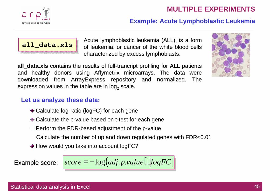
Example: Acute Lymphoblastic Leukemia

all_data.xlsall_data.xlsAcute Acute lymphoblasticlymphoblastic leukemia (ALL), is a form leukemia (ALL), is a form of leukemia, or cancer of the white blood cells of leukemia, or cancer of the white blood cells characterized by excess characterized by excess lymphoblastslymphoblasts..

all_data.xlsall_data.xls contains the results of fullcontains the results of full--trancripttrancript profiling for ALL patients profiling for ALL patients and healthy donors using and healthy donors using AffymetrixAffymetrix microarrays. The data were microarrays. The data were downloaded from downloaded from ArrayExpressArrayExpress repository and normalized. The repository and normalized. The expression values in the table are in logexpression values in the table are in log22 scale.scale.

Let us analyze these data:

Calculate log-ratio (logFC) for each gene

Calculate the p-value based on t-test for each gene

Perform the FDR-based adjustment of the p-value.

Calculate the number of up and down regulated genes with FDR<0.01

How would you take into account logFC?

Example score:Example score: ( ) logFCvaluepadjscore ⋅−= ..log



tetraspanin 7

4.00

5.00

6.00

7.00

8.00

9.00

10.00

11.00

12.00

ALL

ALL

ALL

ALL

ALL

ALL

ALL

ALL

ALL

ALL

ALL

ALL

ALL

ALL

ALL

ALL

ALL

ALL

ALL

ALL

ALL

ALL

ALL

ALL

ALL

ALL

ALL

ALL

ALL

ALL

ALL

ALL

ALL

ALL

ALL

ALL

ALL

ALL

ALL

norm

alno

rmal

norm

alno

rmal

norm

alno

rmal

norm

alno

rmal

norm

alno

rmal

norm

alno

rmal

norm

alno

rmal

norm

alno

rmal

look for "tetraspanin 7" + leukemia in google ☺

Results are never perfectResults are never perfect……


Empirical Interval Estimation Empirical Interval Estimation for Random Functionsfor Random Functions


INTERVAL ESTIMATIONS FOR RANDOM FUNCTIONS

Sum and Square of Normal Variables

Distribution of sum or difference of 2 normal random variablesThe sum/difference of 2 (or more) normal random variables is a normal random variable with mean equal to sum/difference of the means and variance equal to SUM of the variances of the compounds.

Distribution of sum or difference of 2 normal Distribution of sum or difference of 2 normal random variablesrandom variablesThe sum/difference of 2 (or more) normal random The sum/difference of 2 (or more) normal random variables is a normal random variable with variables is a normal random variable with mean mean equal to sum/differenceequal to sum/difference of the means and of the means and variance variance equal to equal to SUMSUM of the variances of the compounds.of the variances of the compounds.

Distribution of sum of squares on k standard normal random variablesThe sum of squares of k standard normal random variables is a χ2 with k degree of freedom.

Distribution of sum of squares on Distribution of sum of squares on kk standard standard normal random variablesnormal random variablesThe sum of squares of The sum of squares of k k standardstandard normal random normal random variables is a variables is a χχ22 with with kk degree of freedomdegree of freedom..

[ ] [ ] [ ]222yxyx

yExEyxE

ondistributiNormalyx

σσσ +=

±=±

→±

±

kfdwithx

ondistributiNormalxxifk

ii

k

=→

→

∑=

..

,...,

2

1

2

1

χ

What to do in more complex situations? What to do in more complex situations? What to do in more complex situations?

?→y

x?→x ( ) ?log →x



Terrifying Theory

Try to solve analytically?Try to solve analytically?Try to solve analytically? Simplest case. E[x] = E[y] = 0Simplest case. Simplest case. E[xE[x] = ] = E[yE[y] = 0] = 0



Practical Approach

Two rates where measured for a PCR experiment: experimental value (X) and control (Y). 5 replicates where performed for each.

From previous experience we know that the error between replicates is normally distributed.

Q1: provide an interval estimation for the fold change X/Y (α=0.05)

Q2: provide an interval estimation for the log fold change log2(X/Y)

Two rates where measured for a PCR experiment: Two rates where measured for a PCR experiment: experimental value (X) and control (Y). 5 replicates experimental value (X) and control (Y). 5 replicates where performed for each.where performed for each.

From previous experience we know that the error From previous experience we know that the error between replicates is normally distributed.between replicates is normally distributed.

Q1:Q1: provide an interval estimation for the fold provide an interval estimation for the fold change X/Y (change X/Y (αα=0.05=0.05))

Q2:Q2: provide an interval estimation for the log fold provide an interval estimation for the log fold change logchange log22(X/Y)(X/Y)

# Experiment Control1 215 832 253 753 198 624 225 915 240 70

Let us use a Let us use a numerical simulationnumerical simulation ……

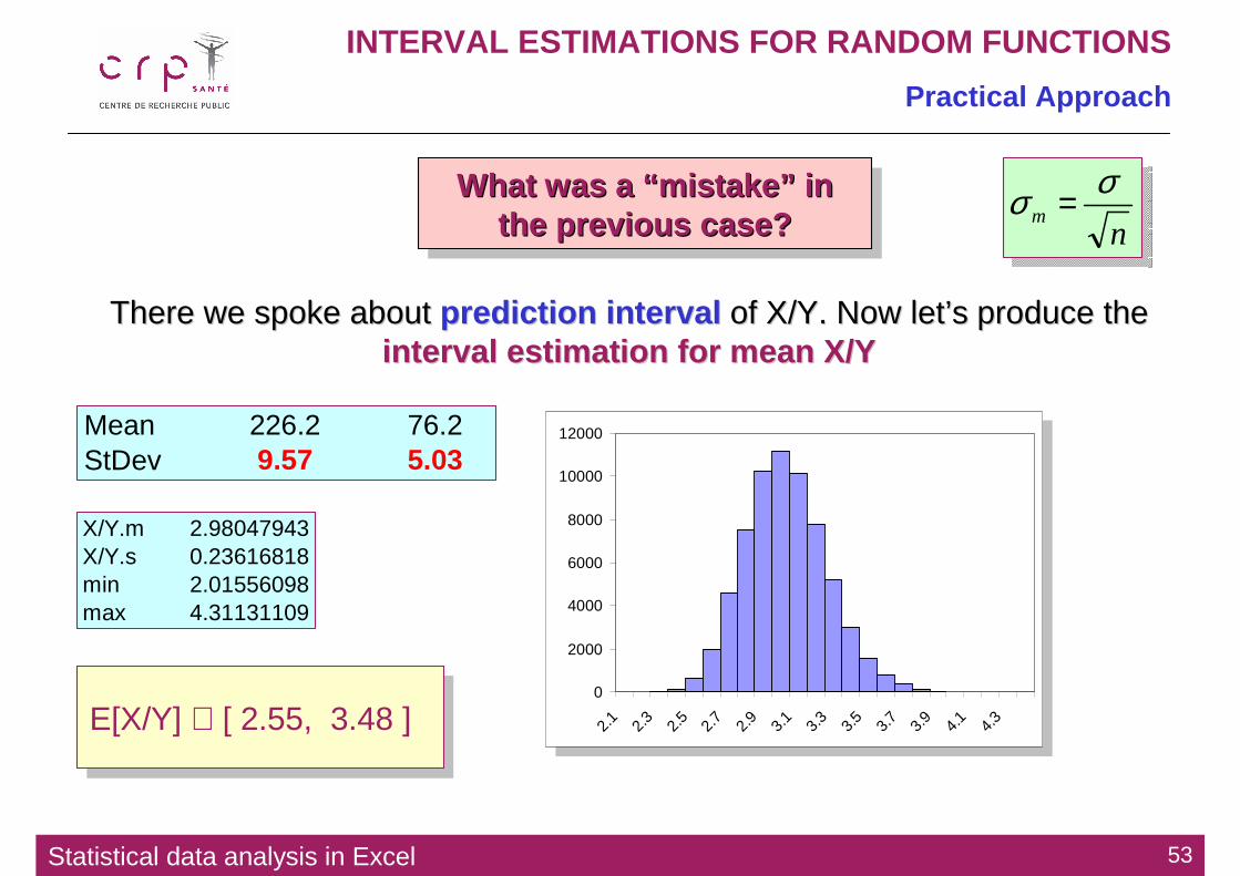
Mean 226.2 76.2StDev 21.39 11.26



Practical Approach

1.1. Generate 2 sets of 65536 normal random variable with Generate 2 sets of 65536 normal random variable with means and standard deviations corresponding to ones of means and standard deviations corresponding to ones of experimental and control set.experimental and control set.

Mean 226.2 76.2StDev 21.39 11.26

In Excel go: Tools →→→→ Data Analysis:

Random Number Generation

If you do not have Data Analysis tool If you do not have Data Analysis tool ––approximate normal distribution by sum of approximate normal distribution by sum of uniform:uniform:

−+= ∑

=

6)(),,(12

1iixxxx xUmmxN σσ

= RAND() ←←←← U(x)



Practical Approach

1.1. Generate 2 sets of 65536 normal random variable Generate 2 sets of 65536 normal random variable with means and standard deviations corresponding to with means and standard deviations corresponding to ones of experimental and control set.ones of experimental and control set.

Mean 226.2 76.2StDev 21.39 11.26

sim.m 226.088799 76.2823sim.s 21.379652 11.2885

2.2. Build the target function. For Q1 build X/YBuild the target function. For Q1 build X/Y

3.3. Study the target function. Calculate summary, build histogram. Study the target function. Calculate summary, build histogram.

X/Y.m 3.03289298X/Y.s 0.566865min -8.14098141max 7.72162205

0

2000

4000

6000

8000

10000

12000

14000

1 1.5 2 2.5 3 3.5 4 4.5 5 5.5 6 6.5 7

4.4. If you would like to have 95% interval, If you would like to have 95% interval, calculate 2.5% and 97.5% percentiles. calculate 2.5% and 97.5% percentiles.

In Excel use function

=PERCENTILE(data,0.025)

X/Y ∈ [ 2.13, 4.33 ] X/Y ∈ [ 2.13, 4.33 ]



Practical Approach

What was a “mistake” in the previous case?

What was a What was a ““ mistakemistake ”” in in the previous case?the previous case?

There we spoke about There we spoke about prediction intervalprediction interval of X/Y. Now letof X/Y. Now let’’s produce the s produce the interval estimation for mean X/Yinterval estimation for mean X/Y

Mean 226.2 76.2StDev 9.57 5.03

0

2000

4000

6000

8000

10000

12000

2.1

2.3

2.5

2.7

2.9

3.1

3.3

3.5

3.7

3.9

4.1

4.3

0

2000

4000

6000

8000

10000

12000

2.1

2.3

2.5

2.7

2.9

3.1

3.3

3.5

3.7

3.9

4.1

4.3E[X/Y] ∈ [ 2.55, 3.48 ] E[X/Y] ∈ [ 2.55, 3.48 ]

X/Y.m 2.98047943X/Y.s 0.23616818min 2.01556098max 4.31131109

nm

σσ =



Practical Approach

E[log(X/Y)] ∈ [ 1.35, 1.80 ] E[log(X/Y)] ∈ [ 1.35, 1.80 ]

Q2:Q2: provide an interval estimation for the log fold change log2(X/Yprovide an interval estimation for the log fold change log2(X/Y))

0

2000

4000

6000

8000

10000

12000

1 1.1 1.2 1.3 1.4 1.5 1.6 1.7 1.8 1.9 2 2.1

Mean 1.571052Standard Deviation0.113705

Simulation Normal2.50% 1.3546 1.3482

97.50% 1.7998 1.7939


Goodness of Fit and Goodness of Fit and Independence Independence


TEST OF GOODNESS OF FIT

Multinomial Population

Multinomial population A population in which each element is assigned to one and only one of several categories. The multinomial distribution extends the binomial distribution from two to three or more outcomes.

Multinomial population A population in which each element is assigned to one and only one of several categories. The multinomial distribution extends the binomial distribution from two to three or more outcomes.

The proportions for 3 “classes” of patients with and without treatment are:

Experimental Control

ne=200 nc=100

Are the proportions significantly differentin control and experimental groups?

The proportions for 3 The proportions for 3 ““classesclasses”” of patients of patients with and without treatment are:with and without treatment are:

Experimental ControlExperimental Control

nnee=200 =200 nncc=100 =100

Are the proportions Are the proportions significantly differentsignificantly differentin control and experimental groups? in control and experimental groups?

21%

32%

47%

21%

32%

47%38%

34%

28%38%

34%

28%



ne=200 nc=100




nnee=200 =200 nncc=100 =100


21%

32%

47%

21%

32%

47%38%

34%

28%38%

34%

28%

The new treatment for a disease is tested on 200 patients. The new treatment for a disease is tested on 200 patients. The outcomes are classified as:The outcomes are classified as:

A A –– patient is patient is completely treatedcompletely treatedB B –– disease transforms into a disease transforms into a chronic formchronic formCC –– treatment is treatment is unsuccessfulunsuccessful ��

In parallel the 100 patients treated with standard methods In parallel the 100 patients treated with standard methods are observed are observed

Contingency table = CrosstabulationContingency tables or crosstabulationsare used to record, summarize and analyze the relationship between two or more categorical (usually) variables.

Contingency table = CrosstabulationContingency tables or crosstabulationsare used to record, summarize and analyze the relationship between two or more categorical (usually) variables.

Category Experimental ControlA 94 38B 42 28C 64 34

Sum 200 100



Goodness of Fit



ne=200 nc=100




nnee=200 =200 nncc=100 =100


21%

32%

47%

21%

32%

47%38%

34%

28%38%

34%

28%



ne=200 nc=100




nnee=200 =200 nncc=100 =100


21%

32%

47%

21%

32%

47%38%

34%

28%38%

34%

28%

Goodness of fit test A statistical test conducted to determine whether to reject a hypothesized probability distribution for a population.

Goodness of fit test A statistical test conducted to determine whether to reject a hypothesized probability distribution for a population.

Model − our assumption concerning the distribution, which we would like to test.

Model − our assumption concerning the distribution, which we would like to test.

Observed frequency − frequency distribution for experimentally observed data, fi

Observed frequency − frequency distribution for experimentally observed data, fi

Expected frequency − frequency distribution, which we would expect from our model , ei

Expected frequency − frequency distribution, which we would expect from our model , ei

( )∑

=

−=k

i i

ii

e

ef

1

22χ

Test statistics for goodness of fit

χχχχχχχχ22 has has kk−−−−−−−−11 degree of freedomdegree of freedom

Hypotheses for the test:Hypotheses for the test:

H0: the population follows a multinomial distribution with the probabilities, specified by model

Ha: the population does not follow … model

HH00: : the population follows a multinomial distribution the population follows a multinomial distribution with the probabilities, specified by with the probabilities, specified by modelmodel

HHaa: : the population does not follow the population does not follow …… modelmodel At least 5 expected must be in each category!

At least 5 expected must be in each category!



Example

The new treatment for a disease is tested on 200 patients. The new treatment for a disease is tested on 200 patients. The outcomes are classified as:The outcomes are classified as:

A A –– patient is patient is completely treatedcompletely treatedB B –– disease transforms into a disease transforms into a chronic formchronic formCC –– treatment is treatment is unsuccessfulunsuccessful ��

In parallel the 100 patients treated with standard methods In parallel the 100 patients treated with standard methods are observed are observed

1.1. Select the model and calculate expected Select the model and calculate expected frequenciesfrequencies

LetLet’’s use control group (classical s use control group (classical treatment) as a model, then:treatment) as a model, then:

3.3. Calculate Calculate pp--value for value for χχ22 with with d.fd.f. = . = kk−−11

= CHIDIST(χ2,d.f. )

= CHITEST(f, e) p-value = 0.018, reject H 0p-value = 0.018, reject H 0

2.2. Compare expected frequencies with Compare expected frequencies with the experimental ones and build the experimental ones and build χχ22

( )∑

=

−=k

i i

ii

e

ef

1

22χ

CategoryControl

frequenciesModel for

controlExpected freq., e

A 38 0.38 76B 28 0.28 56C 34 0.34 68

Sum 100 1 200

Experimental freq., f

944264200

Category (f-e)2/e

A 4.263B 3.500C 0.235

Chi2 7.998

Category Experimental ControlA 94 38B 42 28C 64 34

Sum 200 100


TEST OF INDEPENDENCE

Goodness of Fit for Independence Test: Example

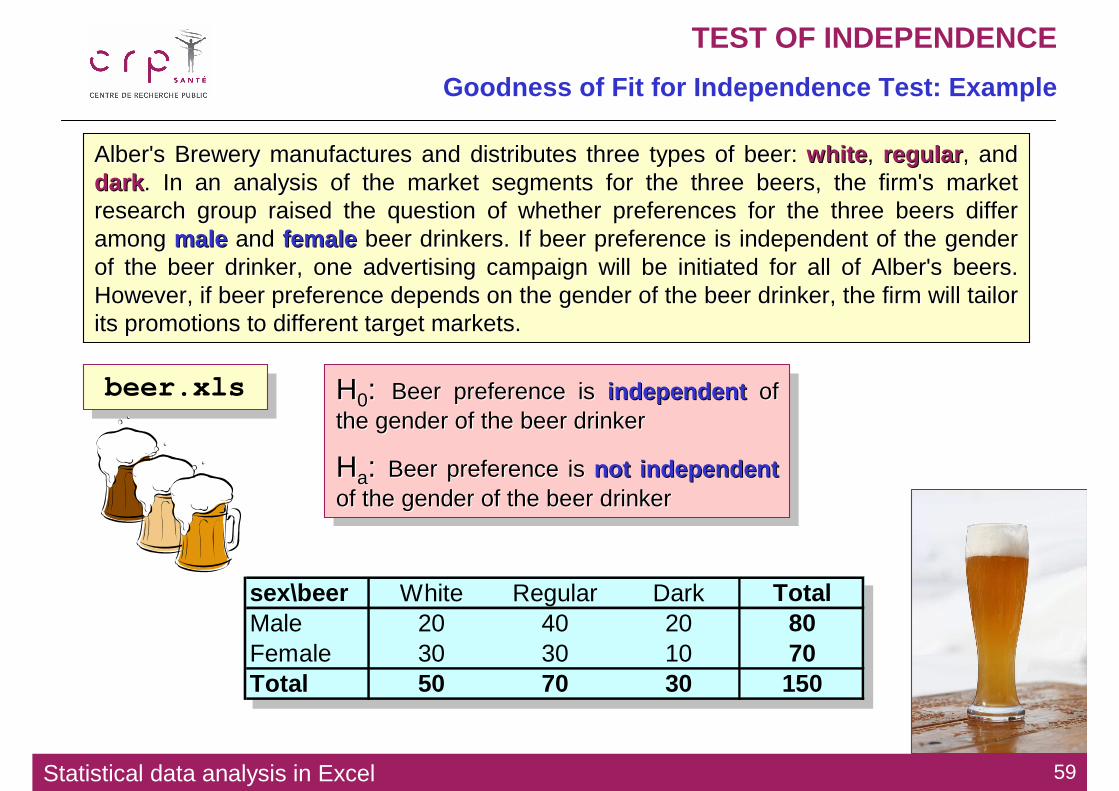
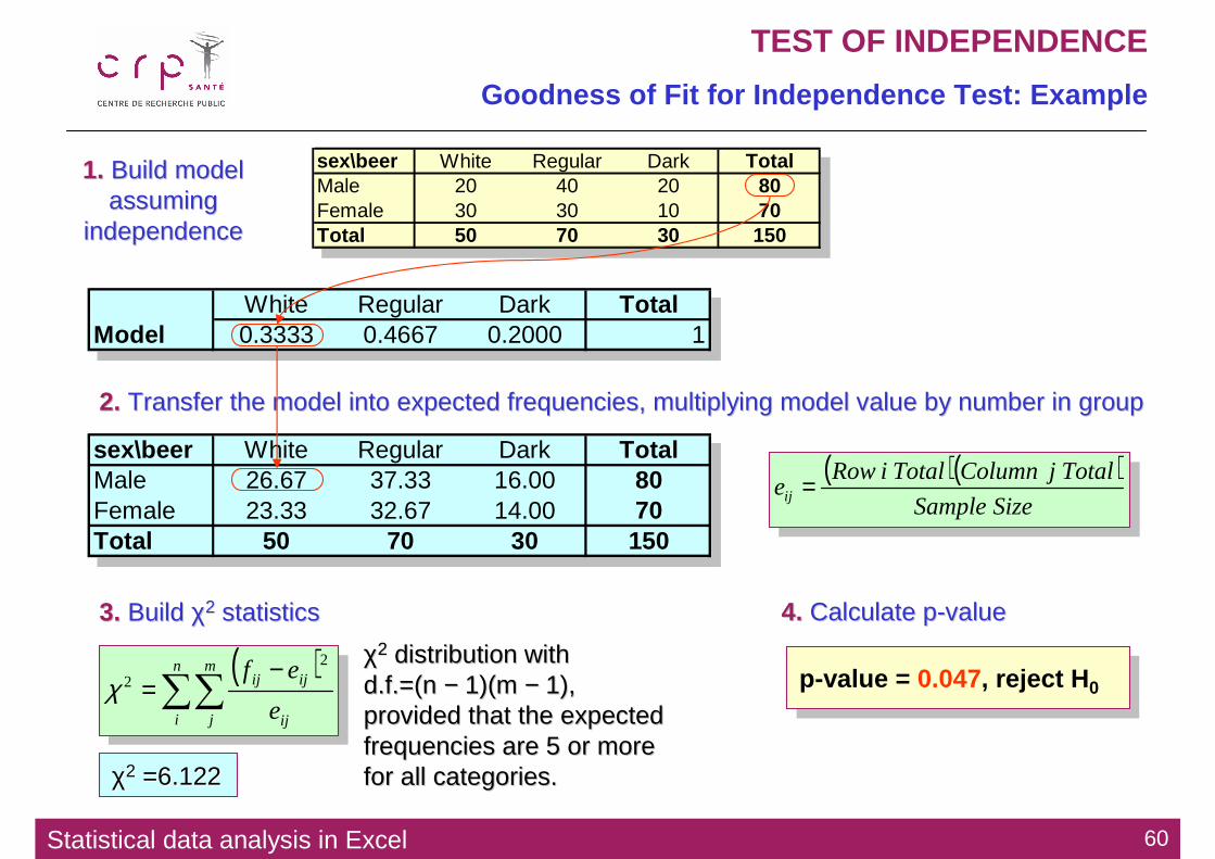
Alber'sAlber's Brewery manufactures and distributes three types of beer: Brewery manufactures and distributes three types of beer: whitewhite , , regularregular , and , and darkdark . In an analysis of the market segments for the three beers, the. In an analysis of the market segments for the three beers, the firm's market firm's market research group raised the question of whether preferences for thresearch group raised the question of whether preferences for the three beers differ e three beers differ among among malemale and and femalefemale beer drinkers. If beer preference is independent of the gender beer drinkers. If beer preference is independent of the gender of the beer drinker, one advertising campaign will be initiated of the beer drinker, one advertising campaign will be initiated for all of for all of Alber'sAlber's beers. beers. However, if beer preference depends on the gender of the beer drHowever, if beer preference depends on the gender of the beer drinker, the firm will tailor inker, the firm will tailor its promotions to different target markets.its promotions to different target markets.

H0: Beer preference is independent of the gender of the beer drinker

Ha: Beer preference is not independentof the gender of the beer drinker

HH00: : Beer preference is Beer preference is independentindependent of of the gender of the beer drinkerthe gender of the beer drinker

HHaa: : Beer preference is Beer preference is not independentnot independentof the gender of the beer drinkerof the gender of the beer drinker

sex\beer White Regular Dark TotalMale 20 40 20 80Female 30 30 10 70Total 50 70 30 150

beer.xlsbeer.xls


TEST OF INDEPENDENCE

Goodness of Fit for Independence Test: Example

White Regular Dark TotalModel 0.3333 0.4667 0.2000 1

sex\beer White Regular Dark TotalMale 20 40 20 80Female 30 30 10 70Total 50 70 30 150

1.1. Build model Build model assuming assuming

independenceindependence

2.2. Transfer the model into expected frequencies, multiplying modelTransfer the model into expected frequencies, multiplying model value by number in groupvalue by number in group

sex\beer White Regular Dark TotalMale 26.67 37.33 16.00 80Female 23.33 32.67 14.00 70Total 50 70 30 150

( )( )SizeSample

TotaljColumnTotaliRoweij =

( )∑∑

−=

n

i

m

j ij

ijij

e

ef 2

2χ

3.3. Build Build χχ22 statisticsstatistics

χχ22 distribution with distribution with d.fd.f.=(.=(nn −− 1)(1)(mm −− 1), 1), provided that the expected provided that the expected frequencies are 5 or more frequencies are 5 or more for all categories.for all categories.χχ22 =6.122=6.122

4.4. Calculate pCalculate p--valuevalue

p-value = 0.047, reject H 0p-value = 0.047, reject H 0


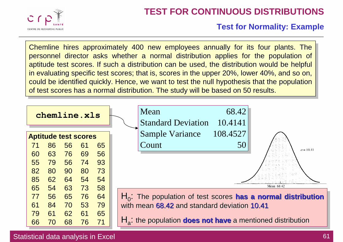
TEST FOR CONTINUOUS DISTRIBUTIONS

Test for Normality: Example

Chemline hires approximately 400 new employees annually for its four plants. The personnel director asks whether a normal distribution applies for the population of aptitude test scores. If such a distribution can be used, the distribution would be helpful in evaluating specific test scores; that is, scores in the upper 20%, lower 40%, and so on, could be identified quickly. Hence, we want to test the null hypothesis that the population of test scores has a normal distribution. The study will be based on 50 results.

ChemlineChemline hires approximately 400 new employees annually for its four plahires approximately 400 new employees annually for its four plants. The nts. The personnel director asks whether a normal distribution applies fopersonnel director asks whether a normal distribution applies for the population of r the population of aptitude test scores. If such a distribution can be used, the diaptitude test scores. If such a distribution can be used, the distribution would be helpful stribution would be helpful in evaluating specific test scores; that is, scores in the upperin evaluating specific test scores; that is, scores in the upper 20%, lower 40%, and so on, 20%, lower 40%, and so on, could be identified quickly. Hence, we want to test the null hypcould be identified quickly. Hence, we want to test the null hypothesis that the population othesis that the population of test scores has a normal distribution. The study will be baseof test scores has a normal distribution. The study will be based on 50 results.d on 50 results.

Aptitude test scores71 86 56 61 6560 63 76 69 5655 79 56 74 9382 80 90 80 7385 62 64 54 5465 54 63 73 5877 56 65 76 6461 84 70 53 7979 61 62 61 6566 70 68 76 71

chemline.xlschemline.xls

H0: The population of test scores has a normal distributionwith mean 68.42 and standard deviation 10.41

Ha: the population does not have a mentioned distribution

HH00: : The population of test scores The population of test scores has a normal distributionhas a normal distributionwith mean with mean 68.4268.42 and standard deviation and standard deviation 10.4110.41

HHaa: : the population the population does not havedoes not have a mentioned distributiona mentioned distribution

Mean 68.42Standard Deviation 10.4141Sample Variance 108.4527Count 50


TEST FOR CONTINUOUS DISTRIBUTIONS

Test for Normality: Example

chemline.xlschemline.xls

Mean 68.42Standard Deviation 10.4141Sample Variance 108.4527Count 50

BinObserved frequency

Expected frequency

55.1 5 559.68 5 563.01 9 565.82 6 568.42 2 571.02 5 573.83 2 577.16 5 581.74 5 5More 6 5Total 50 50

( )∑

=

−=k

i i

ii

e

ef

1

22χ

χχχχ2 distribution with d.f.= n −−−− p −−−− 1,

where p – number of estimated parameters

χχχχχχχχ22 distribution with distribution with d.fd.f .= .= nn −−−−−−−− pp −−−−−−−− 1,1,

where where pp –– number of estimated number of estimated parametersparameters

pp = 2 includes mean and variance= 2 includes mean and varianced.fd.f. = 10 . = 10 −− 2 2 −− 11χχχχχχχχ2 2 = 7.2= 7.2

p-value = 0.41, cannot reject H 0

p-value = 0.41, cannot reject H 0


Thank you for your attention

QUESTIONS ?

Date post:	18-Apr-2020
Category:	Documents
Upload:	others
View:	21 times
Download:	0 times

STATISTICAL DATA ANALYSIS IN...

Documents