Statistical Mechanics of Money, Income, Debt, and...

Statistical mechanics of money, income and wealth Victor Yakovenko 1

Statistical Mechanics of Money, Income, Debt, and Energy Consumption

Victor M. Yakovenko Department of Physics, University of Maryland, College Park, USA

http://www2.physics.umd.edu/~yakovenk/econophysics/

• European Physical Journal B 17, 723 (2000) …………… • Reviews of Modern Physics 81, 1703 (2009) • Book Classical Econophysics (Routledge, 2009) • New Journal of Physics 12, 075032 (2010).

with A. A. Dragulescu, A. C. Silva, A. Banerjee, T. Di Matteo, J. B. Rosser

Outline of the talk • Statistical mechanics of money • Debt and financial instability • Two-class structure of income distribution • Global inequality in energy consumption


“Money, it’s a gas.”

Pink Floyd


Boltzmann-Gibbs versus Pareto distribution

Ludwig Boltzmann (1844-1906) Vilfredo Pareto (1848-1923)

Boltzmann-Gibbs probability distribution P(ε)∝exp(-ε/T), where ε is energy, and T=〈ε〉 is temperature.

Pareto probability distribution P(r)∝1/r(α+1) of income r.

An analogy between the distributions of energy ε and money m or income r


Boltzmann-Gibbs probability distribution of energy

Boltzmann-Gibbs probability distribution P(ε) ∝ exp(−ε/T) of energy ε, where T = 〈ε〉 is temperature. It is universal – independent of model rules, provided the model belongs to the time-reversal symmetry class.

Detailed balance: w12→1’2’P(ε1) P(ε2) = w1’2’→12P(ε1′) P(ε2′)

Collisions between atoms ε1

ε2

ε1′ = ε1 + Δε

ε2′ = ε2 − Δε

Conservation of energy: ε1 + ε2 = ε1′ + ε2′

Boltzmann-Gibbs distribution maximizes entropy S = −Σε P(ε) lnP(ε) under the constraint of conservation law Σε P(ε) ε = const.

Boltzmann-Gibbs probability distribution P(m) ∝ exp(−m/T) of money m, where T = 〈m〉 is the money temperature.

Detailed balance: w12→1’2’P(m1) P(m2) = w1’2’→12P(m1′) P(m2′)

Economic transactions between agents

m1

m2

m1′ = m1 + Δm

m2′ = m2 − Δm

Conservation of money: m1 + m2 = m1′+ m2′

money


Computer simulation of money redistribution

The stationary distribution of money m is exponential: P(m) ∝ e−m/T


Money distribution with debt

Debt per person is limited to 800 units.

Total debt in the system is limited via the Required Reserve Ratio (RRR): Xi, Ding, Wang, Physica A 357, 543 (2005)

•  In practice, RRR is enforced inconsistently and does not limit total debt. • Without a constraint on debt, the system does not have a stationary

equilibrium. •  Free market itself does not have an intrinsic mechanism for limiting

debt, and there is no such thing as the equilibrium debt.


Probability distribution of individual income

US Census data 1996 – histogram and points A

PSID: Panel Study of Income Dynamics, 1992 (U. Michigan) – points B

Distribution of income r is exponential: P(r) ∝ e−r/T


Income distribution in the USA, 1997

Two-class society Upper Class • Pareto power law •  3% of population •  16% of income •  Income > 120 k$: investments, capital

Lower Class • Boltzmann-Gibbs exponential law

•  97% of population •  84% of income •  Income < 120 k$: wages, salaries

“Thermal” bulk and “super-thermal” tail distribution

r*


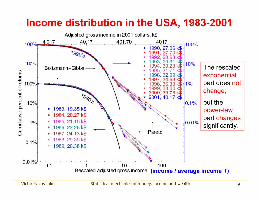
Income distribution in the USA, 1983-2001

The rescaled exponential part does not change,

but the power-law part changes significantly.

(income / average income T)


Income distribution in Sweden

The data plot from Fredrik Liljeros and Martin Hällsten,

Stockholm University


The origin of two classes

 Different sources of income: salaries and wages for the lower class, and capital gains and investments for the upper class.

 Their income dynamics can be described by additive and multiplicative diffusion, correspondingly.

 From the social point of view, these can be the classes of employees and employers, as described by Karl Marx.

 Emergence of classes from the initially equal agents was simulated by Ian Wright “The Social Architecture of Capitalism” Physica A 346, 589 (2005), see also the new book “Classical Econophysics” (2009)


Diffusion model for income kinetics Suppose income changes by small amounts Δr over time Δt. Then P(r,t) satisfies the Fokker-Planck equation for 0<r<∞:

For a stationary distribution, ∂tP = 0 and

For the lower class, Δr are independent of r – additive diffusion, so A and B are constants. Then, P(r) ∝ exp(-r/T), where T = B/A, – an exponential distribution.

For the upper class, Δr ∝ r – multiplicative diffusion, so A = ar and B = br2. Then, P(r) ∝ 1/rα+1, where α = 1+a/b, – a power-law distribution.

For the upper class, income does change in percentages, as shown by Fujiwara, Souma, Aoyama, Kaizoji, and Aoki (2003) for the tax data in Japan. For the lower class, the data is not known yet.


Additive and multiplicative income diffusion If the additive and multiplicative diffusion processes are present simultaneously, then A= A0+ar and B= B0+br2 = b(r0

2+r2). The stationary solution of the FP equation is

It interpolates between the exponential and the power-law distributions and has 3 parameters:

 T = B0/A0 – the temperature of the exponential part

 α = 1+a/b – the power-law exponent of the upper tail

  r0 – the crossover income between the lower and upper parts.

Yakovenko (2007) arXiv:0709.3662, Fiaschi and Marsili (2007) preprint online


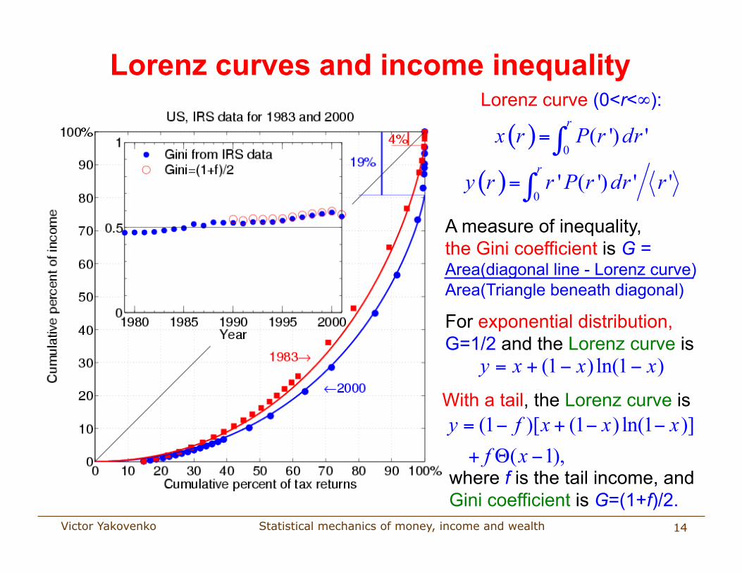
A measure of inequality, the Gini coefficient is G = Area(diagonal line - Lorenz curve) Area(Triangle beneath diagonal)

Lorenz curves and income inequality Lorenz curve (0<r<∞):

With a tail, the Lorenz curve is

where f is the tail income, and Gini coefficient is G=(1+f)/2.

For exponential distribution, G=1/2 and the Lorenz curve is

Statistical mechanics of money, income and wealth Victor Yakovenko

f - fraction of income in the tail <r> − average income in the whole system T − average income in the exponential part

Income inequality peaks during speculative bubbles in financial markets

15

Time evolution of income inequality

Gini coefficient G=(1+f)/2


“The next great depression will be from 2008 to 2023”

Harry S. Dent, book “The Great Boom Ahead”, page 16, published in 1993

His forecast was based on demographic data: The post-war ”baby boomers” generation to invest retirement savings in the stock market massively in the 1990s.

His new book “The Great Depression Ahead”, January 2009


The current financial crisis is not the only and, perhaps, not the most important crises that the mankind faces: •  exhaustion of fossil fuels and other natural resources •  global warming caused by CO2 emissions from fossil fuels

Brief history of the biosphere evolution: •  Plants consume and store energy from the Sun through photosynthesis •  Animals eat plants, which store Sun’s energy •  Animals eat animals, which eat plants, which store Sun’s energy • Humans eat all of the above,

+ consume dead plants and animals (fossil fuels), which store Sun’s energy

•  For thousands of years, the progress of human civilization was biologically limited by muscle energy (of humans or animals) and by wood fuel.

• Couple of centuries ago, the humans discovered how to massively utilize Sun’s energy stored in fossil fuels (coal and oil): the era of industrial revolution and modern capitalism.

•  In a couple of centuries, the humans managed to spend fossil fuels accumulated for millions of years.

• Now this energy binge is coming to an end. Will humankind manage to find a new way for sustainable life? Will new technology save us?


Global inequality in energy consumption

Global distribution of energy consumption per person is roughly exponential.

Division of a limited resource + entropy maximization produce exponential distribution.

Physiological energy consumption of a human at rest is about 100 W


Global inequality in energy consumption

The distribution is getting smoother with time. The gap in energy consumption between developed and developing countries shrinks. The global inequality of energy consumption decreased from 1990 to 2005. The energy consumption distribution is getting closer to the exponential.


Conclusions

  The probability distribution of money is stable and has an equilibrium only when a boundary condition, such as m>0, is imposed.

  When debt is permitted, the distribution of money becomes unstable, unless some sort of a limit on maximal debt is imposed.

  Income distribution in the USA has a two-class structure: exponential (“thermal”) for the great majority (97-99%) of population and power-law (“superthermal”) for the top 1-3% of population.

  The exponential part of the distribution is very stable and does not change in time, except for a slow increase of temperature T (the average income).

  The power-law tail is not universal and was increasing significantly for the last 20 years. It peaked and crashed in 2000 and 2006 with the speculative bubbles in financial markets.

  The global distribution of energy consumption per person is highly unequal and roughly exponential. This inequality is important in dealing with the global energy problems.


Thermal machine in the world economy In general, different countries have different temperatures T, which makes possible to construct a thermal machine:

High T2, developed countries

Low T1, developing countries

Money (energy)

Products

T1 < T2

Prices are commensurate with the income temperature T (the average income) in a country.

Products can be manufactured in a low-temperature country at a low price T1 and sold to a high-temperature country at a high price T2.

The temperature difference T2–T1 is the profit of an intermediary.

In full equilibrium, T2=T1 ⇔ No profit ⇔ “Thermal death” of economy

Money (energy) flows from high T2 to low T1 (the 2nd law of thermodynamics – entropy always increases) ⇔ Trade deficit


Income distribution for two-earner families

The average family income is 2T. The most probable family income is T.


No correlation in the incomes of spouses

Every family is represented by two points (r1, r2) and (r2, r1).

The absence of significant clustering of points (along the diagonal) indicates that the incomes r1 and r2 are approximately uncorrelated.


Time evolution of the tail parameters

• Pareto tail changes in time non-monotonously, in line with the stock market.

• The tail income swelled 5-fold from 4% in 1983 to 20% in 2000.

• It decreased in 2001 with the crash of the U.S. stock market.

The Pareto index α in C(r)∝1/rα is non-universal. It changed from 1.7 in 1983 to 1.3 in 2000.


Lorenz curve and Gini coefficient for families Lorenz curve is calculated for families P2(r)∝r exp(-r/T). The calculated Gini coefficient for families is G=3/8=37.5%

Maximum entropy (the 2nd law of thermodynamics) ⇒ equilibrium inequality: G=1/2 for individuals, G=3/8 for families.

No significant changes in Gini and Lorenz for the last 50 years. The exponential (“thermal”) Boltzmann-Gibbs distribution is very stable, since it maximizes entropy.


Time evolution of income temperature

The nominal average income T doubled: 20 k$ 1983 40 k$ 2001, but it is mostly inflation.


Wealth distribution in the United Kingdom

For UK in 1996, T = 60 k£

Pareto index α = 1.9

Fraction of wealth in the tail f = 16%


World distribution of Gini coefficient

A sharp increase of G is observed in E. Europe and former Soviet Union (FSU) after the collapse of communism – no equilibrium yet.

In W. Europe and N. America, G is close to 3/8=37.5%, in agreement with our theory.

Other regions have higher G, i.e. higher inequality.

The data from the World Bank (B. Milanović)


Income distribution in Australia

The coarse-grained PDF (probability density function) is consistent with a simple exponential fit.

The fine-resolution PDF shows a sharp peak around 7.3 kAU$, probably related to a welfare threshold set by the government.

Date post:	17-Jun-2018
Category:	Documents
Upload:	trandieu
View:	221 times
Download:	0 times

Statistical Mechanics of Money, Income, Debt, and...

Documents