Statistics - Correlation, Linear Regression, And Logistic Regression

C H A P T E R 1 2

Correlation, Linear Regression, and Logistic Regression

Biological phenomena in their numerous phases, economic andsocial, were seen to be only differentiated from the physical bythe intensity of their correlations. The idea Galton placed beforehimself was to represent by a single quantity the degree of rela-tionships, or of partial causality between the different variablesof our everchanging universe.

—Karl Pearson, The Life, Letters, and Labours of Francis Galton,Volume IIIA, Chapter XIV, p. 2

The previous chapter presented various chi-square tests for determining whether ornot two variables that represented categorical measurements were significantly as-sociated. The question arises about how to determine associations between vari-ables that represent higher levels of measurement. This chapter will cover the Pear-son product moment correlation coefficient (Pearson correlation coefficient orPearson correlation), which is a method for assessing the association between twovariables that represent either interval- or ratio-level measurement.

Remember from the previous chapter that examples of interval level measure-ment are Fahrenheit temperature and I.Q. scores; ratio level measures include bloodpressure, serum cholesterol, and many other biomedical research variables thathave a true zero point. In comparison to the chi-square test, the correlation coeffi-cient provides additional useful information—namely, the strength of associationbetween the two variables.

We will also see that linear regression and correlation are related because thereare formulas that relate the correlation coefficient to the slope parameter of the re-gression equation.. In contrast to correlation, linear regression is used for predictingstatus on a second variable (e.g., a dependent variable) when the value of a predic-tor variable (e.g., an independent variable) is known.

Another technique that provides information about the strength of associationbetween a predictor variable (e.g., a risk factor variable) and an outcome variable

Introductory Biostatistics for the Health Sciences, by Michael R. Chernick 251and Robert H. Friis. ISBN 0-471-41137-X. Copyright © 2003 Wiley-Interscience.

cher-12.qxd 1/14/03 9:26 AM Page 251

(e.g., dead or alive) is logistic regression. In the case of a logistic regression analy-sis, the outcome is a dichotomy; the predictor can be selected from variables thatrepresent several levels of measurement (such as categorical or ordinal), as we willdemonstrate in Section 12.9. For example, a physician may use a patient’s totalserum cholesterol value and race to predict high or low levels of coronary heart dis-ease risk.

12.1 RELATIONSHIPS BETWEEN TWO VARIABLES

In Figure 12.1, we present examples of several types of relationships between twovariables. Note that the horizontal and vertical axes are denoted by the symbols Xand Y, respectively.

Both Figures 12.1A and 12.1B represent linear associations, whereas the remain-ing figures illustrate nonlinear associations. Figures 12.1A and 12.1B portray directand inverse linear associations, respectively. The remaining figures represent non-linear associations, which cannot be assessed directly by using a Pearson correla-tion coefficient. To assess these types of associations, we will need to apply otherstatistical methods such as those described in Chapter 14 (nonparametric tests). Inother cases, we can use data transformations, a topic that will be discussed brieflylater in this text.

12.2 USES OF CORRELATION AND REGRESSION

The Pearson correlation coefficient (�), is a population parameter that measures thedegree of association between two variables. It is a natural parameter for a distribu-tion called the bivariate normal distribution. Briefly, the bivariate normal distribu-tion is a probability distribution for X and Y that has normal distributions for both Xand Y and a special form for the density function for the variable pairs. This form al-lows for positive or negative dependence between X and Y.

The Pearson correlation coefficient is used for assessing the linear (straight line)association between an X and a Y variable, and requires interval or ratio measure-ment. The symbol for the sample correlation coefficient is r, which is the sample es-timate of � that can be obtained from a sample of pairs (X, Y) of values for X and Y.The correlation varies from negative one to positive one (–1 � r � +1). A correla-tion of + 1 or –1 refers to a perfect positive or negative X, Y relationship, respective-ly (refer to Figures 12.1A and 12.1B). Data falling exactly on a straight line indi-cates that |r| = 1.

The reader should remember that correlation coefficients merely indicate associ-ation between X and Y, and not causation. If |r| = 1, then all the sample data fall ex-actly on a straight line. This one-to-one association observed for the sample datadoes not necessarily mean that |�| = 1; but if the number of pairs is large, a high val-ue for r suggests that the correlation between the variable pairs in the population ishigh.

252 CORRELATION, LINEAR REGRESSION, AND LOGISTIC REGRESSION

cher-12.qxd 1/14/03 9:26 AM Page 252

253

Fig

ure

12.1

.E

xam

ples

of

biva

riat

e as

soci

atio

ns.

cher-12.qxd 1/14/03 9:26 AM Page 253

Previously, we defined the term “variance” and saw that it is a special parameterof a univariate normal distribution. With respect to correlation and regression, wewill be considering the bivariate normal distribution. Just as the univariate normaldistribution has mean and variance as natural parameters in the density function, sotoo is the correlation coefficient a natural parameter of the bivariate normal distrib-ution. This point will be discussed later in this chapter.

Many biomedical examples call for the use of correlation coefficients: A physi-cian might want to know whether there is an association between total serum cho-lesterol values and triglycerides. A medical school admission committee mightwant to study whether there is a correlation between grade point averages of gradu-ates and MCAT scores at admission. In psychiatry, interval scales are used to mea-sure stress and personality characteristics such as affective states. For example, re-searchers have studied the correlation between Center for Epidemiologic StudiesDepression (CESD) scores (a measure of depressive symptoms) and stressful lifeevents measures.

Regression analysis is very closely related to linear correlation analysis. In fact,we will learn that the formulae for correlation coefficients and the slope of a regres-sion line are similar and functionally related. Thus far we have dealt with bivariateexamples, but linear regression can extend to more than one predictor variable. Thelinearity requirement in the model is for the regression coefficients and not for thepredictor variables. We will provide more information on multiple regression inSection 12.9.

Investigators use regression analysis very widely in the biomedical sciences. Asnoted previously, the researchers use an independent variable to predict a dependentvariable. For example, regression analysis may be used to assess a dose–responserelationship for a drug administered to laboratory animals. The drug dose would beconsidered the independent variable, and the response chosen would be the depen-dent variable. A dose–response relationship is a type of relationship in which in-creasing doses of a substance produce increasing biological responses; e.g., the re-lationship between number of cigarettes consumed and incidence of lung cancer isconsidered to be a dose–response relationship.

12.3 THE SCATTER DIAGRAM

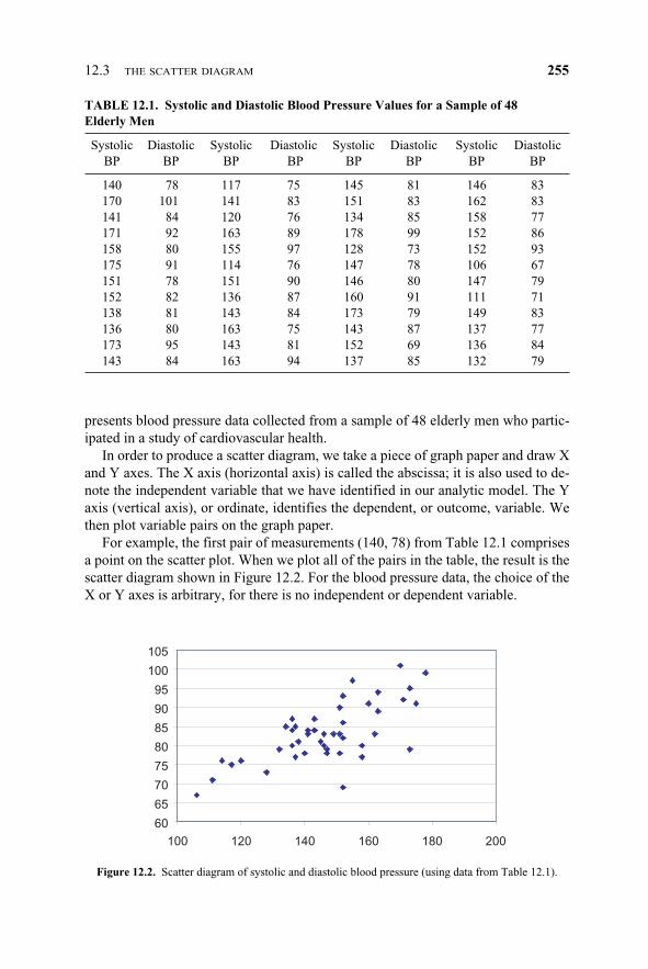
A scatter diagram is used to portray the relationship between two variables; the rela-tionship occurs in a sample of ordered (X, Y) pairs. One constructs such a diagram byplotting, on Cartesian coordinates, X and Y measurements (X and Y pairs) for eachsubject. As an example of two highly correlated measures, consider systolic and di-astolic blood pressure. Remember that when your blood pressure is measured, youare given two values (e.g., 120/70). Across a sample of subjects, these two values areknown to be highly correlated and are said to form a linear (straight line) relationship.

Further, as r decreases, the points on a scatter plot diverge from the line of bestfit. The points form a cloud—a scatter cloud—of dots; two measures that are uncor-related would produce the interior of a circle or an ellipse without tilt. Table 12.1


cher-12.qxd 1/14/03 9:26 AM Page 254

presents blood pressure data collected from a sample of 48 elderly men who partic-ipated in a study of cardiovascular health.

In order to produce a scatter diagram, we take a piece of graph paper and draw Xand Y axes. The X axis (horizontal axis) is called the abscissa; it is also used to de-note the independent variable that we have identified in our analytic model. The Yaxis (vertical axis), or ordinate, identifies the dependent, or outcome, variable. Wethen plot variable pairs on the graph paper.

For example, the first pair of measurements (140, 78) from Table 12.1 comprisesa point on the scatter plot. When we plot all of the pairs in the table, the result is thescatter diagram shown in Figure 12.2. For the blood pressure data, the choice of theX or Y axes is arbitrary, for there is no independent or dependent variable.

12.3 THE SCATTER DIAGRAM 255

TABLE 12.1. Systolic and Diastolic Blood Pressure Values for a Sample of 48 Elderly Men

Systolic Diastolic Systolic Diastolic Systolic Diastolic Systolic Diastolic BP BP BP BP BP BP BP BP

140 78 117 75 145 81 146 83170 101 141 83 151 83 162 83141 84 120 76 134 85 158 77171 92 163 89 178 99 152 86158 80 155 97 128 73 152 93175 91 114 76 147 78 106 67151 78 151 90 146 80 147 79152 82 136 87 160 91 111 71138 81 143 84 173 79 149 83136 80 163 75 143 87 137 77173 95 143 81 152 69 136 84143 84 163 94 137 85 132 79

60

65

70

75

80

85

90

95

100

105

100 120 140 160 180 200

Figure 12.2. Scatter diagram of systolic and diastolic blood pressure (using data from Table 12.1).

cher-12.qxd 1/14/03 9:26 AM Page 255

12.4 PEARSON’S PRODUCT MOMENT CORRELATIONCOEFFICIENT AND ITS SAMPLE ESTIMATE

The formulae for a Pearson sample product moment correlation coefficient (alsocalled a Pearson correlation coefficient) are shown in Equations 12.1 and 12.2. Thedeviation score formula for r is

r = (12.1)

The calculation formula for r is

�n

i=1

XY –

r = ____________________________________ (12.2)

��We will apply these formulae to the small sample of weight and height measure-

ments shown in Table 12.2. The first calculation uses the deviation score formula(i.e., the difference between each observation for a variable and the mean of thevariable).

The data needed for the formulae are shown in Table 12.3. When using the cal-culation formula, we do not need to create difference scores, making the calcula-tions a bit easier to perform with a hand-held calculator.

We would like to emphasize that the Pearson product moment correlation mea-sures the strength of the linear relationship between the variables X and Y. Twovariables X and Y can have an exact non-linear functional relationship, implying aform of dependence, and yet have zero correlation. An example would be the func-tion y = x2 for x between –1 and +1. Suppose that X is uniformly distributed on [0,1] and Y = X2 without any error term. For a bivariate distribution, r is an estimate ofthe correlation (�) between X and Y, where

� =

The covariance between X and Y defined by Cov(X, Y) is E[(X – �x)(Y – �y)], where�x and �y are, respectively, the population means for X and Y. We will show thatCov(X, Y) = 0 and, consequently, � = 0. For those who know calculus, this proof is

Cov(X, Y)��V�ar�(X�)V�ar�(Y�)�

�n

i=1

Y 2 – ��n

i=1

Y2

��n

�n

i=1

X 2 – ��n

i=1

X2

��n

��n

i=1

X��n

i=1

Y��

n

�n

i=1

(X – X�)(Y – Y�)��

��n

i=1

� (�X� –� X��)2��n

i=1

� (�Y� –� Y��)2�


cher-12.qxd 1/14/03 9:26 AM Page 256

12.4 PEARSON’S PRODUCT MOMENT CORRELATION COEFFICIENT 257

TABLE 12.2. Deviation Score Method for Calculating r (Pearson CorrelationCoefficient)

ID Weight (X) (X – X�) (X – X�)2 Height (Y) (Y – Y�) (Y – Y�)2 (X – X�)(Y – Y�)

1 148 –6.10 37.21 64 1.00 1.00 –6.102 172 17.90 320.41 63 0.00 0.00 0.003 203 48.90 2391.21 67 4.00 16.00 195.604 109 –45.10 2034.01 60 –3.00 9.00 135.305 110 –44.10 1944.81 63 0.00 0.00 0.006 134 –20.10 404.01 62 –1.00 1.00 20.107 195 40.90 1672.81 59 –4.00 16.00 –163.608 147 –7.10 50.41 62 –1.00 1.00 7.109 153 –1.10 1.21 66 3.00 9.00 –3.30

10 170 15.90 252.81 64 1.00 1.00 15.90� 1541 9108.90 630 54.00 201.00

X� = 1541/10 = 154.10 Y� = 630/10 = 63.00

r = r = r = = 0.29201.00�701.34

201��(9�1�0�8�.9�0�)(�5�4�)�

�n

i=1

(Xi – X�)(Yi – Y�)��

��n

i=1

�(X�i –� X��)2��n

i=1

�(Y�i –� Y��)2�

TABLE 12.3. Calculation Formula Method for Calculating r (Pearson Correlation Coefficient)

ID Weight (X) X2 Height (Y) Y2 XY

1 148 21,904 64 4,096 9,4722 172 29,584 63 3,969 10,8363 203 41,209 67 4,489 13,6014 109 11,881 60 3,600 6,5405 110 12,100 63 3,969 6,9306 134 17,956 62 3,844 8,3087 195 38,025 59 3,481 11,5058 147 21,609 62 3,844 9,1149 153 23,409 66 4,356 10,098

10 170 28,900 64 4,096 10,880� 1,541 246,577 630 39,744 97,284

�n

i=1

XiYi –

r = _________________________________

� �� r = r = = 0.29

201.00�701.34

97284 – �(1541

1

)

0

(630)�

��

��246577

1

–

0

(1541)2

��39744

1

–

0

(630)2

��

�n

i=1

Yi2 – ��

n

i=1

Yi2

��n

�n

i=1

Xi2 – ��

n

i=1

Xi2

��n

��n

i=1

Xi��n

i=1

Yi��

n

cher-12.qxd 1/14/03 9:26 AM Page 257

shown in Display 12.1. However, understanding this proof is not essential to under-standing the material in this section.

12.5 TESTING HYPOTHESES ABOUT THE CORRELATION COEFFICIENT

In addition to assessing the strength of association between two variables, we needto know whether their association is statistically significant. The test for the signifi-cance of a correlation coefficient is based on a t test. In Section 12.4, we presented r(the sample statistic for correlation) and � (the population parameter for the correla-tion between X and Y in the population).

The test for the significance of a correlation evaluates the null hypothesis (H0)that � = 0 in the population. We assume Y = a + bX + �. Testing � = 0 is the same astesting b = 0. The term � in the equation is called the noise term or error term. It isalso sometimes referred to as the residual term. The assumption required for hy-pothesis testing is that the noise term has a normal distribution with a mean of zeroand unknown variance �2 independent of X. The significance test for Pearson’s cor-relation coefficient is

tdf = �n� –� 2� (12.3)

where df = n – 2; n = number of pairs.Referring to the earlier example presented in Table 12.2, we may test whether

the previously obtained correlation is significant by using the following procedure:

tdf = �n� –� 2� df = 10 – 2 = 8

t = �1�0� –� 2� = �8� = (2.8284) = 0.79

where p = n.s., t critical = 2.306, 2-tailed.

0.29�0.9629

0.29��1� –� (�0�.0�7�2�9�)�

0.29��1� –� (�0�.2�9�)2�

r��1� –� r�2�

r��1� –� r�2�


Display 12.1: Proof of Cov(X, Y) = 0 and �� = 0 for Y = X2

E(X) = 0 since 1

–1xf(x)dx = 0, also E(Y) = E(X 2) = 1

–1x2f (x)dx =1

–1x2(1)dx = �+1

–1=

Cov(X, Y) = E�(X – 0)�Y – � = E[XY] – � E[X] = E[XY] since E[XY] = 0

Now E[XY] = E[X3] since Y = X2 and E[X3] = 1

–1x3f (x)dx = �+1

–1= = 0

14 – (–1)4

��4

x4

�4

2�3

2�3

2�3

x3

�3

cher-12.qxd 1/14/03 9:26 AM Page 258

12.6 CORRELATION MATRIX

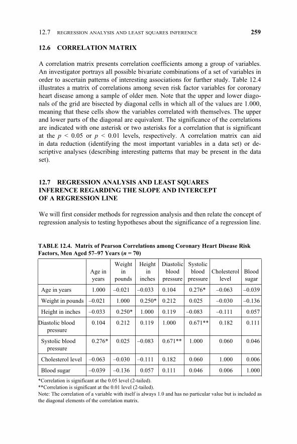
A correlation matrix presents correlation coefficients among a group of variables.An investigator portrays all possible bivariate combinations of a set of variables inorder to ascertain patterns of interesting associations for further study. Table 12.4illustrates a matrix of correlations among seven risk factor variables for coronaryheart disease among a sample of older men. Note that the upper and lower diago-nals of the grid are bisected by diagonal cells in which all of the values are 1.000,meaning that these cells show the variables correlated with themselves. The upperand lower parts of the diagonal are equivalent. The significance of the correlationsare indicated with one asterisk or two asterisks for a correlation that is significantat the p < 0.05 or p < 0.01 levels, respectively. A correlation matrix can aidin data reduction (identifying the most important variables in a data set) or de-scriptive analyses (describing interesting patterns that may be present in the dataset).

12.7 REGRESSION ANALYSIS AND LEAST SQUARES INFERENCE REGARDING THE SLOPE AND INTERCEPT OF A REGRESSION LINE

We will first consider methods for regression analysis and then relate the concept ofregression analysis to testing hypotheses about the significance of a regression line.

12.7 REGRESSION ANALYSIS AND LEAST SQUARES INFERENCE 259

TABLE 12.4. Matrix of Pearson Correlations among Coronary Heart Disease RiskFactors, Men Aged 57–97 Years (n = 70)

Weight Height Diastolic Systolic Age in in in blood blood Cholesterol Blood years pounds inches pressure pressure level sugar

Age in years 1.000 –0.021 –0.033 0.104 0.276* –0.063 –0.039

Weight in pounds –0.021 1.000 0.250* 0.212 0.025 –0.030 –0.136

Height in inches –0.033 0.250* 1.000 0.119 –0.083 –0.111 0.057

Diastolic blood 0.104 0.212 0.119 1.000 0.671** 0.182 0.111pressure

Systolic blood 0.276* 0.025 –0.083 0.671** 1.000 0.060 0.046pressure

Cholesterol level –0.063 –0.030 –0.111 0.182 0.060 1.000 0.006

Blood sugar –0.039 –0.136 0.057 0.111 0.046 0.006 1.000

*Correlation is significant at the 0.05 level (2-tailed).**Correlation is significant at the 0.01 level (2-tailed).Note: The correlation of a variable with itself is always 1.0 and has no particular value but is included asthe diagonal elements of the correlation matrix.

cher-12.qxd 1/14/03 9:26 AM Page 259

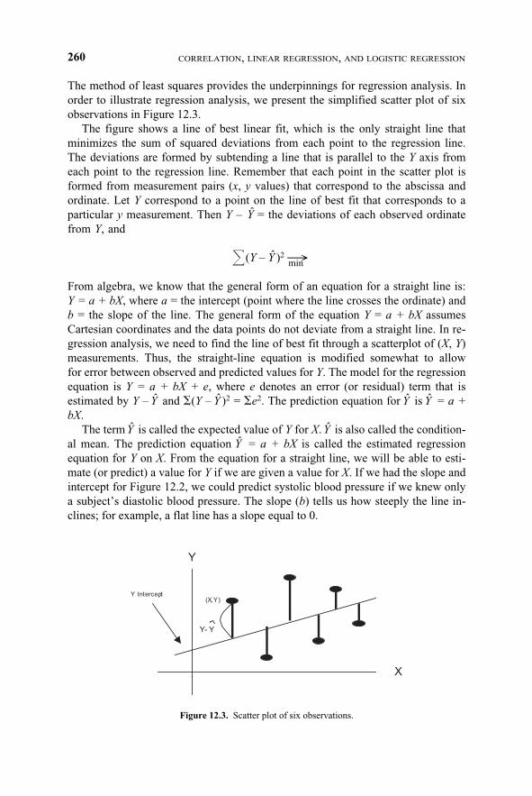
The method of least squares provides the underpinnings for regression analysis. Inorder to illustrate regression analysis, we present the simplified scatter plot of sixobservations in Figure 12.3.

The figure shows a line of best linear fit, which is the only straight line thatminimizes the sum of squared deviations from each point to the regression line.The deviations are formed by subtending a line that is parallel to the Y axis fromeach point to the regression line. Remember that each point in the scatter plot isformed from measurement pairs (x, y values) that correspond to the abscissa andordinate. Let Y correspond to a point on the line of best fit that corresponds to aparticular y measurement. Then Y – Y = the deviations of each observed ordinatefrom Y, and

�(Y – Y )2 �min

From algebra, we know that the general form of an equation for a straight line is:Y = a + bX, where a = the intercept (point where the line crosses the ordinate) andb = the slope of the line. The general form of the equation Y = a + bX assumesCartesian coordinates and the data points do not deviate from a straight line. In re-gression analysis, we need to find the line of best fit through a scatterplot of (X, Y)measurements. Thus, the straight-line equation is modified somewhat to allowfor error between observed and predicted values for Y. The model for the regressionequation is Y = a + bX + e, where e denotes an error (or residual) term that isestimated by Y – Y and �(Y – Y )2 = �e2. The prediction equation for Y is Y = a +bX.

The term Y is called the expected value of Y for X. Y is also called the condition-al mean. The prediction equation Y = a + bX is called the estimated regressionequation for Y on X. From the equation for a straight line, we will be able to esti-mate (or predict) a value for Y if we are given a value for X. If we had the slope andintercept for Figure 12.2, we could predict systolic blood pressure if we knew onlya subject’s diastolic blood pressure. The slope (b) tells us how steeply the line in-clines; for example, a flat line has a slope equal to 0.


Figure 12.3. Scatter plot of six observations.

Y

Y Intercept

X

Y- Y

(X,Y)

cher-12.qxd 1/14/03 9:26 AM Page 260

Substituting for Y in the sums of squares about the regression line gives �(Y – Y )2

= �(Y – a – bX)2. We will not carry out the proof. However, solving for b, it can bedemonstrated that the slope is

b = (12.4)

Note the similarity between this formula and the deviation score formula for rshown in Section 12.4. The equation for a correlation coefficient is

r =

This equation contains the term �ni=1(Yi – Y�)2 in the denominator whereas the formu-

la for the regression equation does not. Using the formula for sample variance, wemay define

Sy2 = �

n

i=1

and

Sy2 = �

n

i=1

The terms sy and sx are simply the square roots of these respective terms. Alterna-tively, b = (Sy/Sx)r. The formulas for estimated y and the y-intercept are:

estimated y(Y ): Y = a + bX� intercept (a): a = X� – bX�

In some instances, it may be easier to use the calculation formula for a slope, asshown in Equation 12.5:

�n

i=1

XiYi –

b = __________________ (12.5)

�n

i=1

Xi2 –

��n

i=1

Yi2

�n

�n

i=1

Xi �n

i=1

Yi

��n

(Xi – X�)2

�n – 1

(Yi – Y�)2

�n – 1

�n

i=1

(Xi – X�)(Yi – Y�)��

��n

i=1

�(X�i –� X��)2��n

i=1

�(Y�i –� Y��)2�

�n

i=1

(Xi – X�)(Yi – Y�)��

�n

i=1

(Xi – X�)2


cher-12.qxd 1/14/03 9:26 AM Page 261

In the following examples, we will demonstrate sample calculations using boththe deviation and calculation formulas. From Table 12.2 (deviation score method):

�(X – X�)(Y – Y�) = 201 �(X – X�)2 = 9108.90

b = = 0.0221

From Table 12.3 (calculation formula method):

�XY = 97,284 �X�Y = (1541)(630) n = 10 �X2 = 246,577

b = b = 0.0221

Thus, both formulas yield exactly the same values for the slope. Solving for the y-intercept (a), a = Y – bX� = 63 – (0.0221)(154.10) = 59.5944.

The regression equation becomes Y = 59.5944 + 0.0221x or, alternatively, height= 59.5944 + 0.0221 weight. For a weight of 110 pounds we would expect height =59.5944 + 0.0221(110) = 62.02 inches.

We may also make statistical inferences about the specific height estimate thatwe have obtained. This process will require several additional calculations, includ-ing finding differences between observed and predicted values for Y, which areshown in Table 12.5.

We may use the information in Table 12.5 to determine the standard error of theestimate of a regression coefficient, which is used for calculation of a confidenceinterval about an estimated value of Y(Y ). Here the problem is to derive a confi-

97,284 – �(1541

1

)

0

(630)�

��

246,577 – �(15

1

4

0

1)2

�

201�9108.90


TABLE 12.5. Calculations for Inferences about Predicted Y and Slope

Predicted Weight (X) X – X� (X – X�)2 Height (Y) Height (Y ) Y – Y (Y – Y )2

148 –6.1 37.21 64 62.8652 1.1348 1.287771172 17.9 320.41 63 63.3956 –0.3956 0.156499203 48.9 2391.21 67 64.0807 2.9193 8.522312109 –45.1 2034.01 60 62.0033 –2.0033 4.013211110 –44.1 1944.81 63 62.0254 0.9746 0.949845134 –20.1 404.01 62 62.5558 –0.5558 0.308914195 40.9 1672.81 59 63.9039 –4.9039 24.04824147 –7.1 50.41 62 62.8431 –0.8431 0.710818153 –1.1 1.21 66 62.9757 3.0243 9.14639170 15.9 252.81 64 63.3514 0.6486 0.420682

Total 1541 9108.9 49.56468

cher-12.qxd 1/14/03 9:26 AM Page 262

dence interval about a single point estimate that we have made for Y. The calcula-tions involve the sum of squares for error (SSE), the standard error of the estimate(sy,x), and the standard error of the expected Y for a given value of x [SE(Y )]. Therespective formulas for the confidence interval about Y are shown in Equation 12.6:

SSE = �(Y – Y )2 sum of squares for error

Sy.x = �� standard error of the estimate (12.6)

SE(Y ) = Sy.x �� +�� standard error of Y for a given value of x

Y ± (tdfn–2)[SE(Y )] is the confidence interval about Y ; e.g., t critical is 100(1 – �/2)percentile of Student’s t distribution with n – 2 degrees of freedom.

The sum of squares for error SSE = �(Y – Y )2 = 49.56468 (from Table 12.5). Thestandard error of the estimate refers to the sample standard deviation associatedwith the deviations about the regression line and is denoted by sy.x:

Sy.x = ��From Table 12.5

Sy.x = �� = 2.7286

The value Sy.x becomes useful for computing a confidence interval about a pre-dicted value of Y. Previously, we determined that the regression equation for pre-dicting height from weight was height = 59.5944 + 0.0221 weight. For a weight of110 pounds we predicted a height of 62.02 inches. We would like to be able to com-pute a confidence interval for this estimate. First we calculate the standard error ofthe expected Y for a given value of [SE(Y )]:

SE(Y ) = Sy.x�� +�� = 2.7286�� +�� –� (�1�5�4�.1�)2� = 0.5599

The 95% confidence interval is

Y ± (tdfn–2)[SE(Y )] 95% CI [62.02 ± 2.306(0.5599)] = [63.31 ↔ 60.73]

We would also like to be able to determine whether the population slope () ofthe regression line is statistically significant. If the slope is statistically significant,there is a linear relationship between X and Y. Conversely, if the slope is not statis-tically significant, we do not have enough evidence to conclude that even a weaklinear relationship exists between X and Y. We will test the following null hypothe-

110�9108.9

1�10

(x – X�)2

�� (Xi – X�)2

1�n

49.56468�

8

SSE�n – 2

(x – X�)2

�� (Xi – X�)2

1�n

SSE�n – 2


cher-12.qxd 1/14/03 9:26 AM Page 263

sis: Ho: = 0. Let b = estimated population slope for X and Y. The formula for esti-mating the significance of a slope parameter is shown in Equation 12.7.

t = = test statistic for the significance of

(12.7)

SE(b) = standard error of the slope estimate [SE(b)]

The standard error of the slope estimate [SE(b)] is (note: refer to Table 12.5 andthe foregoing sections for the values shown in the formula)

SE(b) = = 0.02859 t = = 0.77 p = n.s.

In agreement with the results for the significance of the correlation coefficient,these results suggest that the relationship between height and weight is not statisti-cally significant These two tests (i.e., for the significance of r and significance of b)are actually mathematically equivalent.

This t statistic also can be used to obtain a confidence interval for the slope, name-ly [b – t1–�/2 SE(b), b + t1–�/2 SE(b)], where the critical value for t is the 100(1 – �/2)percentile for Student’s t distribution with n – 2 degrees of freedom. This interval isa 100(1 – �)% confidence interval for .

Sometimes we have knowledge to indicate that the intercept is zero. In suchcases, it makes sense to restrict the solution to the value a = 0 and arrive at the leastsquares estimate for b with this added restriction. The formula changes but is easilycalculated and there exist computer algorithms to handle the zero intercept case.

When the error terms are assumed to have a normal distribution with a mean of 0and a common variance �2, the least squares solution also has the property of maxi-mizing the likelihood. The least squares estimates also have the property of beingthe minmum variance unbiased estimates of the regression parameters [see Draperand Smith (1998) page 137]. This result is called the Gauss–Markov theorem [seeDraper and Smith (1998) page 136].

12.8 SENSITIVITY TO OUTLIERS, OUTLIER REJECTION, AND ROBUST REGRESSION

Outliers refer to unusual or extreme values within a data set. We might expect manybiochemical parameters and human characteristics to be normally distributed, withthe majority of cases falling between ±2 standard deviations. Nevertheless, in alarge data set, it is possible for extreme values to occur. These extreme values maybe caused by actual rare events or by measurement, coding, or data entry errors. Wecan visualize outliers in a scatter diagram, as shown in Figure 12.4.

The least squares method of regression calculates “b” (the regression slope) and“a” (the intercept) by minimizing the sum of squares [�(Y – Y )2] about the regres-

0.0221�0.02859

2.7286��9�1�0�8�.9�

Sy.x��(X�i –� X��)2�

b�SE(b)

b – �SE(b)


cher-12.qxd 1/14/03 9:26 AM Page 264

sion line. Outliers cause distortions in the estimates obtained by the least squaresmethod. Robust regression techniques are used to detect outliers and minimize theirinfluence in regression analyses.

Even a few outliers may impact both the intercept and the slope of a regressionline. This strong impact of outliers comes about because the penalty for a deviationfrom the line of best fit is the square of the residual. Consequently, the slope and in-tercept need to be placed so as to give smaller deviations to these outliers than tomany of the more “normal” observations.

The influence of outliers also depends on their location in the space defined bythe distribution of measurements for X (the independent variable). Observations forvery low or very high values of X are called leverage points and have large effectson the slope of the line (even when they are not outliers). An alternative to leastsquares regression is robust regression, which is less sensitive to outliers than is theleast squares model. An example of robust regression is median regression, a typeof quantile regression, which is also called a minimum absolute deviation model.

A very dramatic example of a major outlier was the count of votes for PatrickBuchanan in Florida’s Palm Beach County in the now famous 2000 presidentialelection. Many people believe that Buchanan garnered a large share of the votesthat were intended for Gore. This result could have happened because of the confus-ing nature of the so-called butterfly ballot.

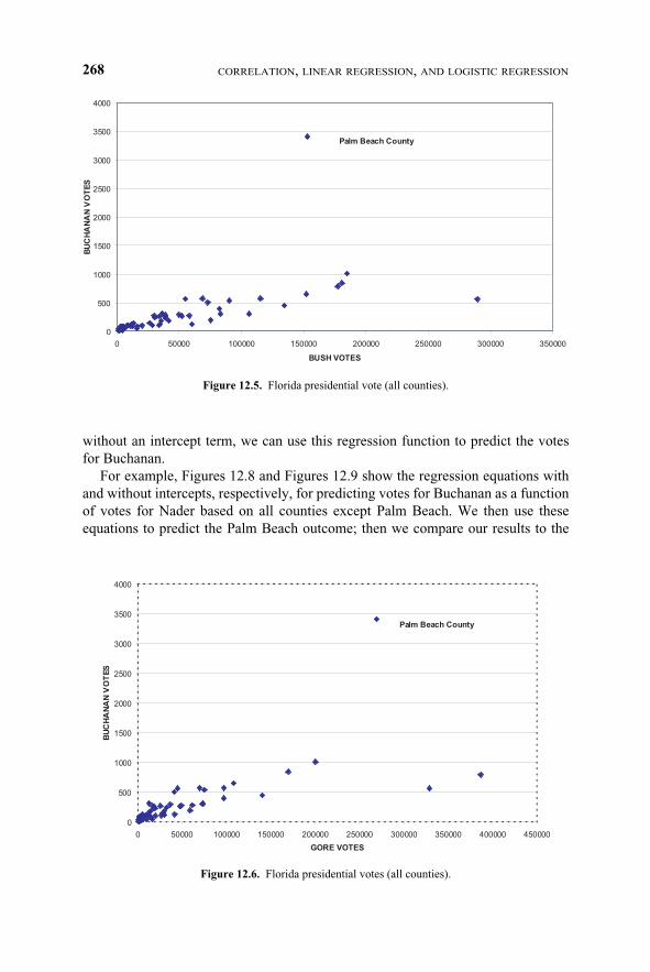
In any case, an inspection of two scatter plots (one for vote totals by county forBuchanan versus Bush, Figure 12.5, and one for vote totals by county for Buchananversus Gore, Figure 12.6) reveals a consistent pattern that enables one to predict thenumber of votes for Buchanan based on the number of votes for Bush or Gore. Thisprediction model would work well in every county except Palm Beach, where thevotes for Buchanan greatly exceeded expectations. Palm Beach was a very obviousoutlier. Let us look at the available data published over the Internet.

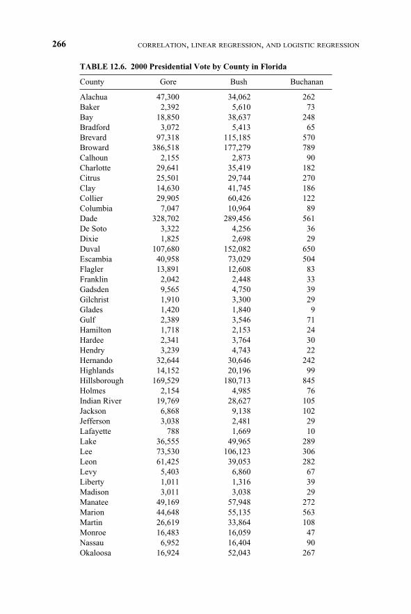
Table 12.6 shows the counties and the number of votes that Bush, Gore, andBuchanan received in each county. The number of votes varied largely by the sizeof the county; however, from a scatter plot you can see a reasonable linear relation-

12.8 SENSITIVITY TO OUTLIERS, OUTLIER REJECTION, AND ROBUST REGRESSION 265

Plot of Most Values

Outliers

Figure 12.4. Scatter diagram with outliers.

cher-12.qxd 1/14/03 9:26 AM Page 265


TABLE 12.6. 2000 Presidential Vote by County in Florida

County Gore Bush Buchanan

Alachua 47,300 34,062 262Baker 2,392 5,610 73Bay 18,850 38,637 248Bradford 3,072 5,413 65Brevard 97,318 115,185 570Broward 386,518 177,279 789Calhoun 2,155 2,873 90Charlotte 29,641 35,419 182Citrus 25,501 29,744 270Clay 14,630 41,745 186Collier 29,905 60,426 122Columbia 7,047 10,964 89Dade 328,702 289,456 561De Soto 3,322 4,256 36Dixie 1,825 2,698 29Duval 107,680 152,082 650Escambia 40,958 73,029 504Flagler 13,891 12,608 83Franklin 2,042 2,448 33Gadsden 9,565 4,750 39Gilchrist 1,910 3,300 29Glades 1,420 1,840 9Gulf 2,389 3,546 71Hamilton 1,718 2,153 24Hardee 2,341 3,764 30Hendry 3,239 4,743 22Hernando 32,644 30,646 242Highlands 14,152 20,196 99Hillsborough 169,529 180,713 845Holmes 2,154 4,985 76Indian River 19,769 28,627 105Jackson 6,868 9,138 102Jefferson 3,038 2,481 29Lafayette 788 1,669 10Lake 36,555 49,965 289Lee 73,530 106,123 306Leon 61,425 39,053 282Levy 5,403 6,860 67Liberty 1,011 1,316 39Madison 3,011 3,038 29Manatee 49,169 57,948 272Marion 44,648 55,135 563Martin 26,619 33,864 108Monroe 16,483 16,059 47Nassau 6,952 16,404 90Okaloosa 16,924 52,043 267

cher-12.qxd 1/14/03 9:26 AM Page 266

ship between; for instance, the total number of votes for Bush and the total numberfor Buchanan. One could form a regression equation to predict the total number ofvotes for Buchanan given that the total number of votes for Bush is known. PalmBeach County stands out as a major exception to the pattern. In this case, we havean outlier that is very informative about the problem of the butterfly ballots.

Palm Beach County had by far the largest number of votes for Buchanan (3407votes). The county that had the next largest number of votes was Pinellas County,with only 1010 votes for Buchanan. Although Palm Beach is a large county,Broward and Dade are larger; yet, Buchanan gained only 789 and 561 votes, re-spectively, in the latter two counties.

Figure 12.5 shows a scatterplot of the votes for Bush versus the votes forBuchanan. From this figure, it is apparent that Palm Beach County is an outlier.

Next, in Figure 12.6 we see the same pattern we saw in Figure 12.5 when com-paring votes for Gore to votes for Buchanan, and in Figure 12.7, votes for Nader tovotes for Buchanan. In each scatter plot, the number of votes for any candidate isproportional to the size of each county, with the exception of Palm Beach County.We will see that the votes for Nader correlate a little better with the votes forBuchanan than do the votes for Bush or for Gore; and the votes for Bush correlatesomewhat better with the votes for Buchanan than do the votes for Gore. If we ex-clude Palm Beach County from the scatter plot and fit a regression function with or


TABLE 12.6. Continued

County Gore Bush Buchanan

Okeechobee 4,588 5,058 43Orange 140,115 134,476 446Osceola 28,177 26,216 145Palm Beach 268,945 152,846 3,407Pasco 69,550 68,581 570Pinellas 200,212 184,884 1,010Polk 74,977 90,101 538Putnam 12,091 13,439 147Santa Rosa 12,795 36,248 311Sarasota 72,854 83,100 305Seminole 58,888 75,293 194St. Johns 19,482 39,497 229St. Lucie 41,559 34,705 124Sumter 9,634 12,126 114Suwannee 4,084 8,014 108Taylor 2,647 4,051 27Union 1,399 2,326 26Volusia 97,063 82,214 396Wakulla 3,835 4,511 46Walton 5,637 12,176 120Washington 2,796 4,983 88

cher-12.qxd 1/14/03 9:26 AM Page 267

without an intercept term, we can use this regression function to predict the votesfor Buchanan.

For example, Figures 12.8 and Figures 12.9 show the regression equations withand without intercepts, respectively, for predicting votes for Buchanan as a functionof votes for Nader based on all counties except Palm Beach. We then use theseequations to predict the Palm Beach outcome; then we compare our results to the


0

500

1000

1500

2000

2500

3000

3500

4000

0 50000 100000 150000 200000 250000 300000 350000

BUSH VOTES

BUCHANANVOTES

Palm Beach County

Figure 12.5. Florida presidential vote (all counties).

0

500

1000

1500

2000

2500

3000

3500

4000

0 50000 100000 150000 200000 250000 300000 350000 400000 450000

GORE VOTES

BUCHANANVOTES

Palm Beach County

Figure 12.6. Florida presidential votes (all counties).

cher-12.qxd 1/14/03 9:26 AM Page 268

3407 votes that actually were counted in Palm Beach County as votes forBuchanan.

Since Nader received 5564 votes in Palm Beach County, we derive, using theequation in Figure 12.8, the prediction of Y for Buchanan: Y = 0.1028(5564) +68.93 = 640.9092. Or, if we use the zero intercept formula, we have Y = 0.1194(5564) = 664.3416.

Similar predictions for the votes for Buchanan using the votes for Bush as the


y = 0.1028x + 68.93

R2= 0.8209

0

200

400

600

800

1000

1200

0 2000 4000 6000 8000 10000 12000

NADER VOTES

BUCHANANVOTES

Figure 12.8. Florida presidential vote (Palm Beach county omitted).

0

500

1000

1500

2000

2500

3000

3500

4000

0 2000 4000 6000 8000 10000 12000

NADERVOTES

BUCHANANVOTES

Palm Beach County

Figure 12.7. Florida presidential votes (all counties).

cher-12.qxd 1/14/03 9:26 AM Page 269

covariate X give the equations Y = 0.0035 X + 65.51 = 600.471 and Y = 0.004 X =611.384 (zero intercept formula), since Bush reaped 152,846 votes in Palm BeachCounty. Votes for Gore also could be used to predict the votes for Buchanan, al-though the correlation is lower (r = 0.7940 for the equation with intercept, and r =0.6704 for the equation without the intercept).

Using the votes for Gore, the regression equations are Y = 0.0025 X + 109.24 andY = 0.0032 X, respectively, for the fit with and without the intercept. Gore’s 268,945votes in Palm Beach County lead to predictions of 781.6025 and 1075.78 using theintercept and nonintercept equations, respectively.

In all cases, the predictions of votes for Buchanan ranged from around 600 votesto approximately 1076 votes—far less than the 3407 votes that Buchanan actuallyreceived. This discrepancy between the number of predicted and actual votes leadsto a very plausible argument that at least 2000 of the votes awarded to Buchanancould have been intended for Gore.

An increase in the number of votes for Gore would eliminate the outlier with re-spect to the number of votes cast for Buchanan that were detected for Palm BeachCounty. This hypothetical increase would be responsive to the complaints of manyvoters who said they were confused by the butterfly ballot. A study of the ballotshows that the punch hole for Buchanan could be confused with Gore’s but not withthat of any other candidate. A better prediction of the vote for Buchanan could beobtained by multiple regression. We will review the data again in Section 12.9.

The undo influence of outliers on regression equations is one of the problemsthat can be resolved by using robust regression techniques. Many texts on regres-sion models are available that cover robust regression and/or the regression diag-nostics that can be used to determine when the assumptions for least squares regres-sion do not apply. We will not go into the details of these topics; however, in


y = 0.1194x

R2= 0.7569

0

200

400

600

800

1000

1200

1400

0 2000 4000 6000 8000 10000 12000

NADER VOTES

BUCHANANVOTES

Figure 12.9. Florida presidential vote (Palm Beach county omitted).

cher-12.qxd 1/14/03 9:26 AM Page 270

Section 12.12 (Additional Reading), we provide the interested reader with severalgood texts. These texts include Chatterjee and Hadi (1988); Chatterjee, Price, andHadi (1999); Ryan (1997); Montgomery, and Peck (1992); Myers (1990); Draper,and Smith (1998); Cook (1998); Belsley, Kuh, and Welsch (1980); Rousseeuw andLeroy (1987); Bloomfield and Steiger (1983); Staudte and Sheather (1990); Cookand Weisberg (1982); and Weisberg (1985).

Some of the aforementioned texts cover diagnostic statistics that are useful fordetecting multicollinearity (a problem that occurs when two or more predictor vari-ables in the regression equation have a strong linear interrelationship). Of course,multicollinearity is not a problem when one deals only with a single predictor.When relationships among independent and dependent variables seem to be nonlin-ear, transformation methods sometimes are employed. For these methods, the leastsquares regression model is fitted to the data after the transformation [see Atkinson(1985) or Carroll and Ruppert (1988)].

As is true of regression equations, outliers can adversely affect estimates of thecorrelation coefficient. Nonparametric alternatives to the Pearson product momentcorrelation exist and can be used in such instances. One such alternative, calledSpearman’s rho, is covered in Section 14.7.

12.9 GALTON AND REGRESSION TOWARD THE MEAN

Francis Galton (1822–1911), an anthropologist and adherent of the scientific beliefsof his cousin Charles Darwin, studied the heritability of such human characteristicsas physical traits (height and weight) and mental attributes (personality dimensionsand mental capabilities). Believing that human characteristics could be inherited, hewas a supporter of the eugenics movement, which sought to improve human beingsthrough selective mating.

Given his interest in how human traits are passed from one generation to thenext, he embarked in 1884 on a testing program at the South Kensington Museumin London, England. At his laboratory in the museum, he collected data from fa-thers and sons on a range of physical and sensory characteristics. He observedamong his study group that characteristics such as height and weight tended to beinherited. However, when he examined the children of extremely tall parents andthose of extremely short parents, he found that although the children were tall orshort, they were closer to the population average than were their parents. Fatherswho were taller than the average father tended to have sons who were taller than av-erage. However, the average height of these taller than average sons tended to belower than the average height of their fathers. Also, shorter than average fatherstended to have shorter than average sons; but these sons tended to be taller on aver-age than their fathers.

Galton also conducted experiments to investigate the size of sweet pea plantsproduced by small and large pea seeds and observed the same phenomenon for asuccessive generation to be closer to the average than was the previous generation.This finding replicated the conclusion that he had reached in his studies of humans.

12.9 GALTON AND REGRESSION TOWARD THE MEAN 271

cher-12.qxd 1/14/03 9:26 AM Page 271

Galton coined the term “regression,” which refers to returning toward the aver-age. The term “linear regression” got its name because of Galton’s discovery of thisphenomenon of regression toward the mean. For more specific information on thistopic, see Draper and Smith (1998), page 45.

Returning to the relationship that Galton discovered between the height at adult-hood of a father and his son, we will examine more closely the phenomenon of re-gression toward the mean. Galton was one of the first investigators to create a scat-ter plot in which on one axis he plotted heights of fathers and on the other, heightsof sons. Each single data point consisted of height measurements of one father–sonpair. There was clearly a high positive correlation between the heights of fathersand the heights of their sons. He soon realized that this association was a mathemat-ical consequence of correlation between the variables rather than a consequence ofheredity.

The paper in which Galton discussed his findings was entitled “Regression to-ward mediocrity in hereditary stature.” His general observations were as follows:Galton estimated a child’s height as

Y = Y� +

where Y is the predicted or estimated child’s height, Y� is the average height of thechildren, X is the parent’s height for that child, and X� is the average height of allparents. Apparently, the choice of X was a weighted average of the mother’s and fa-ther’s heights.

From the equation you can see that if the parent has a height above the mean forparents, the child also is expected to have a greater than average height among thechildren, but the increase Y = Y� is only 2/3 of the predicted increase of the parentover the average for the parents. However, the interpretation that the children’sheights tend to move toward mediocrity (i.e., the average) over time is a fallacysometimes referred to as the regression fallacy.

In terms of the bivariate normal distribution, if Y represents the son’s height andX the parent’s height, and the joint distribution has mean �x for X, mean �y for Y,standard deviation �x for X, standard deviation �y for Y, and correlation �xy betweenX and Y, then E(Y – �y|X = x) = �xy �y (x – �x)/�x.

If we assume �x = �y, the equation simplifies to �xy(x – �x). The simplified equa-tion shows mathematically how the phenomenon of regression occurs, since 0 < �xy

< 1. All of the deviations of X about the mean must be reduced by the multiplier �xy,which is usually less than 1. But the interpretation of a progression toward medioc-rity is incorrect. We see that our interpretation is correct if we switch the roles of Xand Y and ask what is the expected value of the parent’s height (X) given the son’sheight (Y), we find mathematically that E(X – �x|Y = y) = �xy �x(y – �y)/�y, where�y is the overall mean for the population of the sons. In the case when �x = �y, theequation simplifies to �xy(y – �y). So when y is greater than �y, the expected valueof X moves closer to its overall mean (�x) than Y does to its overall mean (�y).

2(X – X�)�

3


cher-12.qxd 1/14/03 9:26 AM Page 272

Therefore, on the one hand we are saying that tall sons tend to be shorter thantheir tall fathers, whereas on the other hand we say that tall fathers tend to be short-er than their tall sons. The prediction for heights of sons based on heights of fathersindicates a progression toward mediocrity; the prediction of heights of fathers basedon heights of sons indicates a progression away from mediocrity. The fallacy lies inthe interpretation of a progression. The sons of tall fathers appear to be shorter be-cause we are looking at (or conditioning on) only the tall fathers. On the other hand,when we look at the fathers of tall sons we are looking at a different group becausewe are conditioning on the tall sons. Some short fathers will have tall sons and sometall fathers will have short sons. So we err when we equate these conditioning sets.The mathematics is correct but our thinking is wrong. We will revisit this fallacyagain with students’ math scores.

When trends in the actual heights of populations are followed over several gen-erations, it appears that average height is increasing over time. Implicit in the re-gression model is the contradictory conclusion that the average height of the popu-lation should remain stable over time. Despite the predictions of the regressionmodel, we still observe the regression toward the mean phenomenon with each gen-eration of fathers and sons.

Here is one more illustration to reinforce the idea that interchanging the predic-tor and outcome variables may result in different conclusions. Michael Chernick’sson Nicholas is in the math enrichment program at Churchville Elementary Schoolin Churchville, Pennsylvania. The class consists of fifth and sixth graders, who takea challenging test called the Math Olympiad test. The test consists of five problems,with one point given for each correct answer and no partial credit given. The possi-ble scores on any exam are 0, 1, 2, 3, 4, and 5. In order to track students’ progress,teachers administer the exam several times during the school year. As a project forthe American Statistical Association poster competition, Chernick decided to lookat the regression toward the mean phenomenon when comparing the scores on oneexam with the scores on the next exam.

Chernick chose to compare 33 students who took both the second and third ex-ams. Although the data are not normally distributed and are very discrete, the linearmodel provides an acceptable approximation; using these data, we can demonstratethe regression toward the mean phenomenon. Table 12.7 shows the individual stu-dent’s scores and the average scores for the sample for each test.

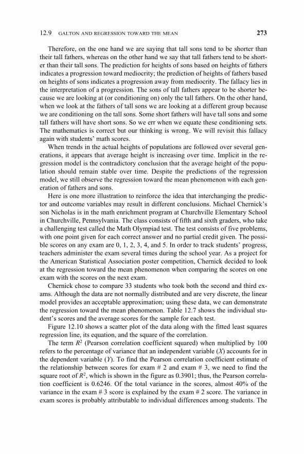
Figure 12.10 shows a scatter plot of the data along with the fitted least squaresregression line, its equation, and the square of the correlation.

The term R2 (Pearson correlation coefficient squared) when multiplied by 100refers to the percentage of variance that an independent variable (X) accounts for inthe dependent variable (Y). To find the Pearson correlation coefficient estimate ofthe relationship between scores for exam # 2 and exam # 3, we need to find thesquare root of R2, which is shown in the figure as 0.3901; thus, the Pearson correla-tion coefficient is 0.6246. Of the total variance in the scores, almost 40% of thevariance in the exam # 3 score is explained by the exam # 2 score. The variance inexam scores is probably attributable to individual differences among students. The


cher-12.qxd 1/14/03 9:26 AM Page 273

average scores for exam # 2 and exam # 3 are 2.363 and 2.272, respectively (refer toTable 12.7).

In Table 12.8, we use the regression equation shown in Figure 12.10 to predictthe individual exam # 3 scores based on the exam # 2 scores. We also can observethe regression toward the mean phenomenon by noting that for scores of 0, 1, and 2(all below the average of 2.272 for exam # 3), the predicted values for Y are higherthan the actual scores, but for scores of 3, 4, and 5 (all above the mean of 2.272), thepredicted values for Y are lower than the actual scores. Hence, all predicted scores


TABLE 12.7. Math Olympiad Scores

Student Number Exam # 2 Score Exam # 3 Score

1 5 42 4 43 3 14 1 35 4 46 1 17 2 38 2 29 4 4

10 4 311 3 312 5 513 0 114 3 115 3 316 3 217 3 218 1 319 3 220 2 321 3 222 0 223 3 224 3 225 3 226 3 227 2 028 1 229 0 130 2 231 1 132 0 133 1 2

Average score: 2.363 2.272

cher-12.qxd 1/14/03 9:26 AM Page 274

(Y s) for exam # 3 are closer to the overall class mean for exam # 3 than are the ac-tual exam # 2 scores.

Note that a property of the least squares estimate is that if we use x = 2.363, themean for the x’s, then we get an estimate of y = 2.272, the mean of the y’s. So if astudent had a score that was exactly equal to the mean for exam # 2, we would pre-dict that the mean of the exam # 3 scores would be that student’s score for exam # 3.Of course, this hypothetical example cannot happen because the actual scores canbe only integers between 0 and 5.

Although the average scores on exam # 3 are slightly lower than the averagescores on exam # 2. the difference between them is not statistically significant, ac-cording to a paired t test (t = 0.463, df = 32).


y = 0.4986x + 1.0943

R2= 0.3901

0

0.5

1

1.5

2

2.5

3

3.5

4

4.5

5

0 0.5 1 1.5 2 2.5 3 3.5 4 4.5 5

EXAM # 2

EXAM

#3

Figure 12.10. Linear regression of olympiad scores of advanced students predicting exam # 3 fromexam # 2.

TABLE 12.8. Regression toward the Mean Based onPredicting Exam #3 Scores from Exam # 2 Scores

Exam # 2 Score Prediction for Exam # 3

Scores 0 1.0943Below 1 1.5929Mean 2 2.0915Scores 3 2.5901Above 4 3.0887Mean 5 3.5873

cher-12.qxd 1/14/03 9:26 AM Page 275

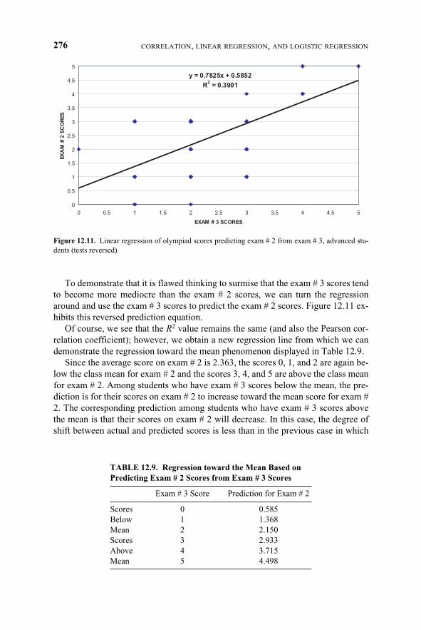
To demonstrate that it is flawed thinking to surmise that the exam # 3 scores tendto become more mediocre than the exam # 2 scores, we can turn the regressionaround and use the exam # 3 scores to predict the exam # 2 scores. Figure 12.11 ex-hibits this reversed prediction equation.

Of course, we see that the R2 value remains the same (and also the Pearson cor-relation coefficient); however, we obtain a new regression line from which we candemonstrate the regression toward the mean phenomenon displayed in Table 12.9.

Since the average score on exam # 2 is 2.363, the scores 0, 1, and 2 are again be-low the class mean for exam # 2 and the scores 3, 4, and 5 are above the class meanfor exam # 2. Among students who have exam # 3 scores below the mean, the pre-diction is for their scores on exam # 2 to increase toward the mean score for exam #2. The corresponding prediction among students who have exam # 3 scores abovethe mean is that their scores on exam # 2 will decrease. In this case, the degree ofshift between actual and predicted scores is less than in the previous case in which


y = 0.7825x + 0.5852

R2= 0.3901

0

0.5

1

1.5

2

2.5

3

3.5

4

4.5

5

0 0.5 1 1.5 2 2.5 3 3.5 4 4.5 5

EXAM # 3 SCORES

EXAM#2SCORES

Figure 12.11. Linear regression of olympiad scores predicting exam # 2 from exam # 3, advanced stu-dents (tests reversed).

TABLE 12.9. Regression toward the Mean Based onPredicting Exam # 2 Scores from Exam # 3 Scores

Exam # 3 Score Prediction for Exam # 2

Scores 0 0.585Below 1 1.368Mean 2 2.150Scores 3 2.933Above 4 3.715Mean 5 4.498

cher-12.qxd 1/14/03 9:26 AM Page 276

exam # 2 scores were used to predict exam # 3 scores. Again, according to an im-portant property of least squares estimates, if we use the exam # 3 mean of 2.272 forx, we will obtain the exam # 2 mean of 2.363 for y (which is exactly the same valuefor the mean of exam # 2 shown in Table 12.7).

Now let’s examine the fallacy of our thinking regarding the trend in exam scorestoward mediocrity. The predicted scores for exam # 3 are closer to the mean scorefor exam # 3 than are the actual scores on exam # 2. We thought that both the lowerpredicted and observed scores on exam # 3 meant a trend toward mediocrity. Butthe predicted scores for exam # 2 based on scores on exam # 3 are also closer to themean of the actual scores on exam # 2 than are the actual scores on exam # 3. Thisfinding indicates a trend away from mediocrity in moving in time from scores onexam # 2 to scores on exam # 3. But this is a contradiction because we observed theopposite of what we thought we would find. The flaw in our thinking that led to thiscontradiction is the mistaken belief that the regression toward the mean phenome-non implies a trend over time.

The fifth and sixth grade students were able to understand that the better studentstended to receive the higher grades and the weaker students the lower grades. Butchance also could play a role in a student’s performance on a particular test. So stu-dents who received a 5 on an exam were probably smarter than the other studentsand also should be expected to do well on the next exam. However, because themaximum possible score was 5, by chance some students who scored 5 on oneexam might receive a score of 4 or lower on the next exam, thus lowering the ex-pected score below 5.

Similarly, a student who earns a score of 0 on a particular exam is probably oneof the weaker students. As it is impossible to earn a score of less than 0, a studentwho scores 0 on the first exam has a chance of earning a score of 1 or higher on thenext exam, raising the expected score above 0. So the regression to the mean phe-nomenon is real, but it does not mean that the class as a group is changing. In fact,the class average could stay the same and the regression toward the mean phenome-non could still be seen.

12.10 MULTIPLE REGRESSION

The only difference between multiple linear regression and simple linear regressionis that the former introduces two or more predictor variables into the predictionmodel, whereas the latter introduces only one. Although we often use a model of Y= � + X for the form of the regression function that relates the predictor (indepen-dent) variable X to the outcome or response (dependent) variable Y, we could alsouse a model such as Y = � + X2 or Y = � + lnX (where ln refers to the log func-tion). The function is linear in the regression parameters � and .

In addition to the linearity requirement for the regression model, the other re-quirement for regression theory to work is that the observed values of Y differ fromthe regression function by an independent random quantity, or noise term (errorvariance term). The noise term has a mean of zero and variance of �2. In addition,

12.10 MULTIPLE REGRESSION 277

cher-12.qxd 1/14/03 9:26 AM Page 277

�2 does not depend on X. Under these assumptions the method of least squares pro-vides estimates a and b for � and , respectively, which have desirable statisticalproperties (i.e., minimum variance among unbiased estimators).

If the noise term also has a normal distribution, then its maximum likelihood es-timator can be obtained. The resulting estimation is known as the Gauss–Markovtheorem, the derivation of which is beyond the scope of the present text. The inter-ested reader can consult Draper and Smith (1998), page 136, and Jaske (1994).

As with simple linear regression, the Gauss–Markov theorem applies to multiplelinear regression. For a simple linear regression, we introduced the concept of anoise, or error, term. The prediction equation for multiple linear regression alsocontains an error term. Let us assume a normally distributed additive error termwith variance that is independent of the predictor variables. The least squares esti-mates for the regression coefficients used in the multiple linear regression modelexist; under certain conditions, they are unique and are the same as the maximumlikelihood estimates [Draper and Smith (1998) page 137].

However, the use of matrix algebra is required to express the least squared esti-mates. In practice, when there are two or more possible variables to include in a re-gression equation, one new issue arises regarding the particular subset of variablesthat should go into the final regression equation. A second issue concerns the prob-lem of multicollinearity, i.e., the predictor variables are so highly intercorrelatedthat they produce instability problems.

In addition, one must assess the correlation between the best fitting linear combi-nation of predictor variables and the response variable instead of just a simple cor-relation between the predictor variable and the response variable. The square of thecorrelation between the set of predictor variables and the response variable is calledR2, the multiple correlation coefficient. The term R2 is interpreted as the percentageof the variance in the response variable that can be explained by the regressionfunction. We will not study multiple regression in any detail but will provide an ex-ample to guide you through calculations and their interpretation.

The term “multicollinearity” refers to a situation in which there is a strong, closeto linear relationship among two or more predictor variables. For example, a predic-tor variable X1 may be approximately equal to 2X2 + 5X3 where X2 and X3 are twoother variables that we think relate to our response variable Y.

To understand the concept of linear combinations, let us assume that we includeall three variables (X1 + X2 + X3) in a regression model and that their relationship isexact. Suppose that the response variable Y = 0.3 X1 + 0.7 X2 + 2.1 X3 + �, where �is normally distributed with mean 0 and variance 1.

Since X1 = 2X2 + 5X3, we can substitute the right-hand side of this equation intothe expression for Y. After substitution we have Y = 0.3(2 X2 + 5X3) + 0.7X2 + 2.1X3

+ � = 1.3X2 + 3.6X3 + �. So when one of the predictors can be expressed as a linearfunction of the other, the regression coefficients associated with the predictor vari-ables do not remain the same. We provided examples of two such expressions: Y =0.3X1 + 0.7X2 + 2.1X3 + � and Y = 0.0X1 + 1.3X2 + 3.6X3 + �. There are an infinitenumber of possible choices for the regression coefficients, depending on the linearcombinations of the predictors.


cher-12.qxd 1/14/03 9:26 AM Page 278

In most practical situations, an exact linear relationship will not exist; even a re-lationship that is close to linear will cause problems. Although there will be (unfor-tunately) a unique least squares solution, it will be unstable. By unstable we meanthat very small changes in the observed values of Y and the X’s can produce drasticchanges in the regression coefficients. This instability makes the coefficients im-possible to interpret.

There are solutions to the problem that is caused by a close linear relationshipamong predictors and the outcome variable. The first solution is to select only asubset of the variables, avoiding predictor variables that are highly interrelated (i.e.,multicollinear). Stepwise regression is a procedure that can help overcome multi-collinearity, as is ridge regression. The topic of ridge regression is beyond the scopeof the present text; the interested reader can consult Draper and Smith (1998),Chapter 17. The problem of multicollinearity is also called “ill-conditioning”; is-sues related to the detection and treatment of regression models that are ill-condi-tioned can be found in Chapter 16 of Draper and Smith (1998). Another approach tomulticollinearity involves transforming the set of X’s to a new set of variables thatare “orthogonal.” Orthogonality, used in linear algebra, is a technique that willmake the X’s uncorrelated; hence, the transformed variables will be well-condi-tioned (stable) variables.

Stepwise regression is one of many techniques commonly found in statistical soft-ware packages for multiple linear regression. The following account illustrates howa typical software package performs a stepwise regression analysis. In stepwise re-gression we start with a subset of the X variables that we are considering for inclusionin a prediction model. At each step we apply a statistical test (often an F test) to de-termine if the model with the new variable included explains a significantly greaterpercentage of the variation in Y than the previous model that excluded the variable.

If the test is significant, we add the variable to the model and go to the next stepof examining other variables to add or drop. At any stage, we may also decide todrop a variable if the model with the variable left out produces nearly the same per-centage of variation explained as the model with the variable entered. The userspecifies critical values for F called the “F to enter” and the “F to drop” (or uses thedefault critical values provided by a software program).

Taking into account the critical values and a list of X variables, the program pro-ceeds to enter and remove variables until none meets the criteria for addition ordeletion. A variable that enters the regression equation at one stage may still be re-moved at another stage, because the F test depends on the set of variables currentlyin the model at a particular iteration.

For example, a variable X may enter the regression equation because it has agreat deal of explanatory power relative to the current set under consideration.However, variable X may be strongly related to other variables (e.g., U, V, and Z)that enter later. Once these other variables are added, the variable X could providelittle additional explanatory information than that contained in variables U, V, andZ. Hence, X is deleted from the regression equation.

In addition to multicollinearity problems, the inclusion of too many variables inthe equation can lead to an equation that fits the data very well but does not do near-


cher-12.qxd 1/14/03 9:26 AM Page 279

ly as well as equations with fewer variables when predicting future values of Ybased on known values of x. This problem is called overfitting. Stepwise regressionis useful because it reduces the number of variables in the regression, helping withoverfitting and multicollinearity problems. However, stepwise regression is not anoptimal subset selection approach; even if the F to enter criterion is the same as theF to leave criterion, the resulting final set of variables can differ from one anotherdepending on the variables that the user specifies for the starting set.

Two alternative approaches to stepwise regression are forward selection andbackward elimination. Forward selection starts with no variables in the equationand adds them one at a time based solely on an F to enter criterion. Backward elim-ination starts with all the variables in the equation and drops variables one at a timebased solely on an F to drop criterion. Generally, statisticians consider stepwise re-gression to be better than either forward selection or backward elimination. Step-wise regression is preferred to the other two techniques because it tends to test moresubsets of variables and generally settles on a better choice than either forward se-lection or backward elimination. Sometimes, the three approaches will lead to thesame subset of variables, but often they will not.

To illustrate multiple regression, we will consider the example of predictingvotes for Buchanan in Palm Beach County based on the number of votes for Nader,Gore, and Bush (refer back to Section 12.7). For all counties except Palm Beach,we fit the model Y = � + 1X1 + 2X2 + 3X3 + �, where X1 represents votes forNader, X2 votes for Bush, and X3 votes for Gore; � is a random noise term withmean 0 and variance �2 that is independent of X1, X2, and X3; and �, 1, 2, and 3

are the regression parameters. We will entertain this model and others with one ofthe predictor variables left out. To do this we will use the SAS procedure REG andwill show you the SAS code and output. You will need a statistical computer pack-age to solve most multiple regression problems. Multiple regression, which can befound in most of the common statistical packages, is one of the most widely usedapplied statistical techniques.

The following three regression models were considered:

1. A model including votes for Nader, Bush, and Gore to predict votes forBuchanan

2. A model using only votes for Nader and Bush to predict votes for Buchanan

3. A model using votes for Nader and Bush and an nteraction term defined asthe product of the votes for Nader and the votes for Bush

The coefficient for votes for Gore in model (1) was not statistically significant, somodel (2) is probably better than (1) for prediction. Model (3) provided a slightly bet-ter fit than model (2), and under model (3) all the coefficients were statistically sig-nificant. The SAS code (presented in italics) used to obtain the results is as follows:

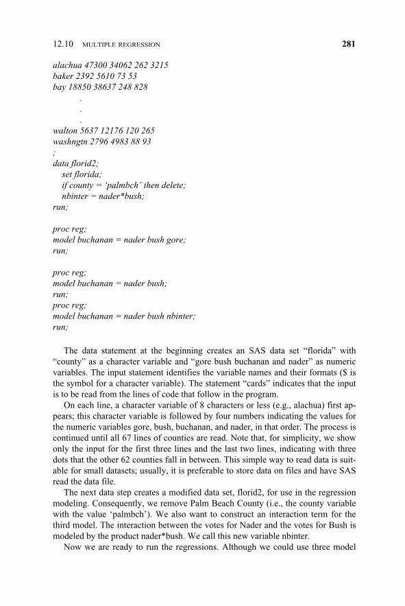
data florida:input county $ gore bush buchanan nader;cards;


cher-12.qxd 1/14/03 9:26 AM Page 280

alachua 47300 34062 262 3215baker 2392 5610 73 53bay 18850 38637 248 828

.

.

.walton 5637 12176 120 265washngtn 2796 4983 88 93;data florid2;

set florida;if county = ‘palmbch’ then delete;nbinter = nader*bush;

run;

proc reg;model buchanan = nader bush gore;run;

proc reg;model buchanan = nader bush;run;proc reg;model buchanan = nader bush nbinter;run;

The data statement at the beginning creates an SAS data set “florida” with“county” as a character variable and “gore bush buchanan and nader” as numericvariables. The input statement identifies the variable names and their formats ($ isthe symbol for a character variable). The statement “cards” indicates that the inputis to be read from the lines of code that follow in the program.

On each line, a character variable of 8 characters or less (e.g., alachua) first ap-pears; this character variable is followed by four numbers indicating the values forthe numeric variables gore, bush, buchanan, and nader, in that order. The process iscontinued until all 67 lines of counties are read. Note that, for simplicity, we showonly the input for the first three lines and the last two lines, indicating with threedots that the other 62 counties fall in between. This simple way to read data is suit-able for small datasets; usually, it is preferable to store data on files and have SASread the data file.

The next data step creates a modified data set, florid2, for use in the regressionmodeling. Consequently, we remove Palm Beach County (i.e., the county variablewith the value ‘palmbch’). We also want to construct an interaction term for thethird model. The interaction between the votes for Nader and the votes for Bush ismodeled by the product nader*bush. We call this new variable nbinter.

Now we are ready to run the regressions. Although we could use three model


cher-12.qxd 1/14/03 9:26 AM Page 281

statements in a single regression procedure, instead we performed the regression asthree separate procedures. The model statement specifies the dependent variable onthe left side of the equation. On the right side of the equation is the list of predictorvariables. For the first regression we have the variables nader, bush, and gore; forthe second just the variables nader and bush. The third regression specifies nader,bush, and their interaction term nbinter.

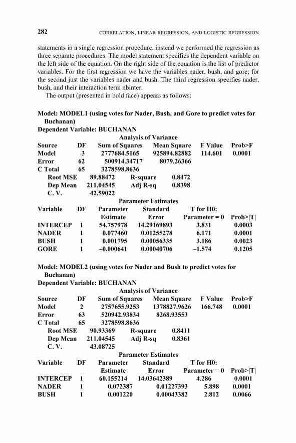
The output (presented in bold face) appears as follows:

Model: MODEL1 (using votes for Nader, Bush, and Gore to predict votes for Buchanan)

Dependent Variable: BUCHANANAnalysis of Variance

Source DF Sum of Squares Mean Square F Value Prob>FModel 3 2777684.5165 925894.82882 114.601 0.0001Error 62 500914.34717 8079.26366C Total 65 3278598.8636

Root MSE 89.88472 R-square 0.8472Dep Mean 211.04545 Adj R-sq 0.8398C. V. 42.59022

Parameter EstimatesVariable DF Parameter Standard T for H0:

Estimate Error Parameter = 0 Prob>|T|INTERCEP 1 54.757978 14.29169893 3.831 0.0003NADER 1 0.077460 0.01255278 6.171 0.0001BUSH 1 0.001795 0.00056335 3.186 0.0023GORE 1 –0.000641 0.00040706 –1.574 0.1205

Model: MODEL2 (using votes for Nader and Bush to predict votes for Buchanan)





Estimate Error Parameter = 0 Prob>|T|INTERCEP 1 60.155214 14.03642389 4.286 0.0001NADER 1 0.072387 0.01227393 5.898 0.0001BUSH 1 0.001220 0.00043382 2.812 0.0066


cher-12.qxd 1/14/03 9:26 AM Page 282

Model: MODEL3 (using votes for Nader and Bush plus an interaction term, Nader*Bush)





Estimate Error Parameter = 0 Prob>|T|INTERCEP 1 36.353406 16.7731503 2.261 0.0273NADER 1 0.098017 0.01512781 6.479 0.0001BUSH 1 0.001798 0.00046703 3.850 0.0003NBINTER 1 –0.000000232 0.00000009 –2.677 0.0095

For each model, the value of R2 describes the percentage of the variance in thevotes for Buchanan that is explained by the predictor variables. By taking into ac-count the joint influence of the significant predictor variables in the model, the ad-justed R2 provides a better measure of goodness of fit than do the individual predic-tors. Both models (1) and (2) have very similar R2 and adjusted R2 values. Model (3)has slightly higher R2 and adjusted R2 values than does either model (1) or model (2).

The F test for each model shows a p-value less than 0.0001 (the column labeledProb>F), indicating that at least one of the regression parameters is different fromzero. The individual t test on the coefficients suggests the coefficients that are dif-ferent from zero. However, we must be careful about the interpretation of these re-sults, due to multiple testing of coefficients.

Regarding model (3), since Bush received 152,846 votes and Nader 5564, theequation predicts that Buchanan should have 659.236 votes. Model (1) uses the268,945 votes for Gore (in addition to those for Nader and Bush) to predict 587.710votes for Buchanan. Model (2) predicts the vote total for Buchanan to be 649.389.Model (3) is probably the best model, for it predicts that the votes for Buchanan willbe less than 660. So again we see that any reasonable model would predict thatBuchanan would receive 1000 or fewer votes, far less than the 3407 he actually re-ceived!

12.11 LOGISTIC REGRESSION

Logistic regression is a method for predicting binary outcomes on the basis of oneor more predictor variables (covariates). The goal of logistic regression is the sameas the goal of ordinary multiple linear regression; we attempt to construct a model

12.11 LOGISTIC REGRESSION 283

cher-12.qxd 1/14/03 9:26 AM Page 283

to best describe the relationship between a response variable and one or more inde-pendent explanatory variables (also called predictor variables or covariates). Just asin ordinary linear regression, the form of the model is linear with respect to the re-gression parameters (coefficients). The only difference that distinguishes logisticregression from ordinary linear regression is the fact that in logistic regression theresponse variable is binary (also called dichotomous), whereas in ordinary linear re-gression it is continuous.

A dichotomous response variable requires that we use a methodology that is verydifferent from the one employed in ordinary linear regression. Hosmer andLemeshow (2000) wrote a text devoted entirely to the methodology and many im-portant applications of handling dichotomous response variables in logistic regres-sion equations. The same authors cover the difficult but very important practicalproblem of model building where a “best” subset of possible predictor variables isto be selected based on data. For more information, consult Hosmer and Lemeshow(2000).

In this section, we will present a simple example along with its solution. Giventhat the response variable Y is binary, we will describe it as a random variable thattakes on either the value 0 or the value 1. In a simple logistic regression equationwith one predictor variable, X, we denote by (x) the probability that the responsevariable Y equals 1 given that X = x. Since Y takes on only the values 0 and 1, thisprobability (x) also is equal to E(Y|X = x) since E(Y|X = x) = 0 P(Y = 0|X = x) + 1P(Y = 1|X = x) = P(Y = 1|X = x) = (x).

Just as in simple linear regression, the regression function for logistic regressionis the expected value of the response variable, given that the predictor variable X =x. As in ordinary linear regression we express this function by a linear relationshipof the coefficients applied to the predictor variables. The linear relationship is spec-ified after making a transformation. If X is continuous, in general X can take on allvalues in the range (–�, +�). However, Y is a dichotomy and can be only 0 or 1.The expectation for Y, given X = x, is that (x) can belong only to [0, 1]. A linearcombination such as � + x can be in (–�, +�) for continuous variables. So we con-sider the logit transformation, namely g(x) = ln[(x)/(1 – (x)]. Here the transfor-mation w(x) = [(x)/(1 – (x)] can take a value from [0, 1] to [0, +�) and ln (thelogarithm to the base e) takes w(x) to (–�, +�). So this logit transformation putsg(x) in the same interval as � + x for arbitrary values of � and .

The logistic regression model is then expressed simply as g(x) = � + x where gis the logit transform of . Another way to express this relationship is on a proba-bility scale by reversing (taking the inverse) the transformations, which gives (x)= exp(� + x)/[1 + exp(� + x)], where exp is the exponential function. This is be-cause the exponential is the inverse of the function ln. That means that exp(ln(x)) =x. So exp[g(x)] = exp(� + x) = exp{ln[(x)/(1 – (x)]} = (x)/1 – (x). We thensolve exp(� + x) = (x)/1 – (x) for (x) and get (x) = exp(� + x)[1 – (x)] =exp(� + x) – exp(� + x)(x). After moving exp(� + x) (x) to the other side ofthe equation, we have (x) + exp(� + x)(x) = exp(� + x) or (x)[1 + exp(� +x)] = exp(� + x). Dividing both sides of the equation by 1 + exp(� + x) at lastgives us (x) = exp(� + x)/[1 + exp(� + x)].


cher-12.qxd 1/14/03 9:26 AM Page 284

The aim of logistic regression is to find estimates of the parameters � and thatbest fit an available set of data. In ordinary linear regression, we based this estima-tion on the assumption that the conditional distribution of Y given X = x was nor-mal. Here we cannot make that assumption, as Y is binary and the error term for Ygiven X = x takes on one of only two values, –(x) when Y = 0 and 1 – (x) when Y= 1 with probabilities 1 – (x) and (x), respectively. The error term has mean zeroand variance [1 – (x)](x). Thus, the error term is just a Bernoulli random variableshifted down by (x).

The least squares solution was used in ordinary linear regression under the usualassumption of constant variance. In the case of ordinary linear regression, we weretold that the maximum likelihood solution was the same as the least squares solu-tion [Draper and Smith (1998), page 137, and discussed in Sections 12.8 and 12.10above]. Because the distribution of error terms is much different for logistic regres-sion than for ordinary linear regression, the least squares solution no longer applies;we can follow the principle of maximizing the likelihood to obtain a sensible solu-tion. Given a set of data (yi, xi) where i = 1, 2, . . . , n and the yi are the observed re-sponses and can have a value of either 0 or 1, and the xi are the corresponding co-variate values, we define the likelihood function as follows:

L(x1, y1, x2, y2, . . . , xn, yn) = (x1)y1[1 – (x1)](1–y1)

(x2)y2[1 – (x2)](1–y2)(x3)y3[1 – (x3)](1–y3), . . . , (xn)yn[1 – (xn)](1–yn) (12.1)

This formula specifies that if yi = 0, then the probability that yi = 0 is 1 – (xi);whereas, if yi = 1, then the probability of yi = 1 is (xi). The expression (xi)yi[1 –(xi)](1–yi) provides a compact way of expressing the probabilities for yi = 0 or yi = 1for each i regardless of the value of y. These terms shown on the right side of theequal sign of Equation 12.8 are multiplied in the likelihood equation because theobserved data are assumed to be independent. To find the maximum values of thelikelihood we solve for � and by simply computing their partial derivatives andsetting them equal to zero. This computation leads to the likelihood equations �[yi –(xi)] = 0 and �xi[yi – (xi)] = 0 which we solve simultaneously for � and . Recallthat in the likelihood equations (xi) = exp(� + xi)/[1 + exp(� + xi)], so the para-meters � and enter the likelihood equations through the terms with (xi).

Generalized linear models are linear models for a function g(x). The function g iscalled the link function. Logistic regression is a special case where the logit func-tion is the link function. See Hosmer and Lemeshow (2000) and McCullagh andNelder (1989) for more details.

Iterative numerical algorithms for generalized linear models are required tosolve maximum likelihood equations. Software packages for generalized linearmodels provide solutions to the complex equations required for logistic regressionanalysis. These programs allow you to do the same things we did with ordinary sim-ple linear regression—namely, to test hypotheses about the coefficients (e.g.,whether or not they are zero) or to construct confidence intervals for the coeffi-cients. In many applications, we are interested only in the predicted values (x) forgiven values of x.

12.11 LOGISTIC REGRESSION 285

cher-12.qxd 1/14/03 9:26 AM Page 285

Table 12.10 reproduces data from Campbell and Machin (1999) regarding he-moglobin levels among menopausal and nonmenopausal women. We use these datain order to illustrate logistic regression analysis.

Campbell and Machin used the data presented in Table 12.10 to construct a lo-gistic regression model, which addressed the risk of anemia among women whowere younger than 30. Female patients who had hemoglobin levels below 12 g/dlwere categorized as anemic. The present authors (Chernick and Friis) dichotomizedthe subjects into anemic and nonanemic in order to examine the relationship of age(under and over 30 years of age) to anemia. (Refer to Table 12.11.)

We note from the data that two out of the five women under 30 years of age wereanemic, while only two out of 15 women over 30 were anemic. None of the womenwho were experiencing menopause was anemic. Due to blood and hemoglobin lossduring menstruation, younger, nonmenopausal women (in comparison tomenopausal women) were hypothesized to be at higher risk for anemia.

In fitting a logistic regression model for anemia as a function of the di-chotomized age variable, Campbell and Machin found that the estimate of the re-gression parameter was 1.4663 with a standard error of 1.1875. The Wald test,analogous to the t test for the significance of a regression coefficient in ordinary lin-ear regression, is used in logistic regression. It also evaluates whether the logistic


TABLE 12.10. Hemoglobin Level (Hb), Packed Cell Volume (PCV), Age, andMenopausal Status for 20 Women*

Menopause Subject Number Hb (g/dl) PCV (%) Age (yrs) (0 = No, 1 = Yes)

1 11.1 35 20 02 10.7 45 22 03 12.4 47 25 04 14.0 50 28 05 13.1 31 28 06 10.5 30 31 07 9.6 25 32 08 12.5 33 35 09 13.5 35 38 0

10 13.9 40 40 011 15.1 45 45 112 13.9 47 49 013 16.2 49 54 114 16.3 42 55 115 16.8 40 57 116 17.1 50 60 117 16.6 46 62 118 16.9 55 63 119 15.7 42 65 120 16.5 46 67 1

*Adapted from Campbell and Machin (1999), page 95, Table 7.1.

cher-12.qxd 1/14/03 9:26 AM Page 286

regression coefficient is significantly different from 0. The value of the Wald statis-tic was 1.5246 for these data (p = 0.2169, n.s.).

With such a small sample size (n = 20) and the dichotomization used, one cannotfind a statistically significant relationship between younger age and anemia. We canalso examine the exponential of the parameter estimate. This exponential is the esti-mated odds ratio (OR), defined elsewhere in this book. The OR turns out to be 4.33,but the confidence interval is very wide and contains 0.

Had we performed the logistic regression using the actual age instead of the di-chotomous values, we would have obtained a coefficient of –0.2077 with a standarderror of 0.1223 for the regression parameter, indicating a decreasing risk of anemiawith increasing age. In this case, the Wald statistic is 2.8837 (p = 0.0895), indicat-ing that the downward trend is statistically significant at the 10% level even for thisrelatively small sample.

12.12 EXERCISES

12.1 Give in your own words definitions of the following terms that pertain to bi-variate regression and correlation:

12.12 EXERCISES 287

TABLE 12.11. Women Reclassified by Age Group and Anemia (Using Datafrom Table 12.10)

Age (0 = under 30, Subject Number Anemic (0 = No, 1 = Yes) 1 = 30 or over)

1 1 02 1 03 0 04 0 05 0 06 1 17 1 18 0 19 0 1

10 0 111 0 112 0 113 0 114 0 115 0 116 0 117 0 118 0 119 0 120 0 1

cher-12.qxd 1/14/03 9:26 AM Page 287

a. Correlation versus associationb. Correlation coefficientc. Regressiond. Scatter diagrame. Slope (b)

12.2 Research papers in medical journals often cite variables that are correlatedwith one another. a. Using a health-related example, indicate what investigators mean when

they say that variables are correlated.b. Give examples of variables in the medical field that are likely to be cor-

related. Can you give examples of variables that are positively correlatedand variables that are negatively correlated?

c. What are some examples of medical variables that are not correlated?Provide a rationale for the lack of correlation among these variables.

d. Give an example of two variables that are strongly related but have acorrelation of zero (as measured by a Pearson correlation coefficient).

12.3 List the criteria that need to be met in order to apply correctly the formulafor the Pearson correlation coefficient.

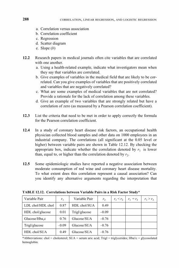
12.4 In a study of coronary heart disease risk factors, an occupational healthphysician collected blood samples and other data on 1000 employees in anindustrial company. The correlations (all significant at the 0.05 level orhigher) between variable pairs are shown in Table 12.12. By checking theappropriate box, indicate whether the correlation denoted by r1 is lowerthan, equal to, or higher than the correlation denoted by r2.

12.5 Some epidemiologic studies have reported a negative association betweenmoderate consumption of red wine and coronary heart disease mortality.To what extent does this correlation represent a causal association? Canyou identify any alternative arguments regarding the interpretation that


TABLE 12.12. Correlations between Variable Pairs in a Risk Factor Study*

Variable Pair r1 Variable Pair r2 r1 < r2 r1 = r2 r1 > r2

LDL chol/HDL chol 0.87 HDL chol/SUA 0.49

HDL chol/glucose 0.01 Trigl/glucose –0.09

Glucose/Hba1c 0.76 Glucose/SUA –0.76

Trigl/glucose –0.09 Glucose/SUA –0.76

HDL chol/SUA 0.49 Glucose/SUA –0.76

*Abbreviations: chol = cholesterol; SUA = serum uric acid; Trigl = triglycerides; Hba1c = glycosolatedhemoglobin.

cher-12.qxd 1/14/03 9:26 AM Page 288

consumption of red wine causes a reduction in coronary heart disease mor-tality?

12.6 A psychiatric epidemiology study collected information on the anxiety anddepression levels of 11 subjects. The results of the investigation are present-ed in Table 12.13. Perform the following calculations:a. Scatter diagramb. Pearson correlation coefficientc. Test the significance of the correlation coefficient at � = 0.05 and � =

0.01.

12.7 Refer to Table 12.1 in Section 12.3. Calculate r between systolic and dias-tolic blood pressure. Calculate the regression equation between systolic anddiastolic blood pressure. Is the relationship statistically significant at the0.05 level?

12.8 Refer to Table 12.14:a. Create a scatter diagram of the relationships between age (X) and choles-

terol (Y), age (X) and blood sugar (Y), and cholesterol (X) and blood sug-ar (Y).

b. Calculate the correlation coefficients (r) between age and cholesterol,age and blood sugar, and cholesterol and blood sugar. Evaluate the sig-nificance of the associations at the 0.05 level.

c. Determine the linear regression equations between age (X) and choles-terol (Y), age (X) and blood sugar (Y), and cholesterol (X) and blood sug-ar (Y). For age 93, what are the estimated cholesterol and blood pressurevalues? What is the 95% confidence interval about these values? Are theslopes obtained for the regression equations statistically significant (atthe 0.05 level)? Do these results agree with the significance of the corre-lations?

12.12 EXERCISES 289

TABLE 12.13. Anxiety and Depression Scores of 11 Subjects

Subject ID Anxiety Score Depression Score

1 24 142 9 53 25 164 26 175 35 226 17 87 49 378 39 419 8 6

10 34 2811 28 33

cher-12.qxd 1/14/03 9:26 AM Page 289

12.9 An experiment was conducted to study the effect on sleeping time of in-creasing the dosage of a certain barbiturate. Three readings were made ateach of three dose levels:

Sleeping Time (Hrs) Dosage (�M/kg)Y X

4 36 35 39 108 107 10

13 1511 159 15

�Y = 72 �X = 84�Y2 = 642 �X2 = 1002�XY = 780

a. Plot the scatter diagram.b. Determine the regression line relating dosage (X) to sleeping time (Y).c. Place a 95% confidence interval on the slope parameter .d. Test at the 0.05 level the hypothesis of no linear relationship between the

two variables.e. What is the predicted sleeping time for a dose of 12 �M/kg?


TABLE 12.14 : Age, Cholesterol Level, and Blood Sugar Level ofElderly Men

Age Cholesterol Blood Sugar

76 80 275 360 125 13976 80 245 238 127 13776 80 245 267 138 13176 63 237 295 129 16093 63 263 245 151 14791 63 251 305 138 13991 64 195 276 137 14897 76 260 275 129 17572 76 245 259 138 15172 76 268 245 139 14772 76 254 226 150 12672 57 282 247 159 129

cher-12.qxd 1/14/03 9:26 AM Page 290

12.10 In the text, a correlation matrix was described. Using your own words, ex-plain what is meant by a correlation matrix. What values appear along thediagonal of a correlation? How do we account for these values?

12.11 An investigator studying the effects of stress on blood pressure subjectedmine monkeys to increasing levels of electric shock as they attempted to ob-tain food from a feeder. At the end of a 2-minute stress period, blood pres-sure was measured. (Initially, the blood pressure readings of the nine mon-keys were essentially the same).

Blood Pressure Shock IntensityY X

125 30130 30120 30150 50145 50160 50175 70180 70180 70

Some helpful intermediate calculations: �X = 450, �Y = 1365, �X2 =24900, �Y2 = 211475, (�X)2 = 202500, (�Y)2 = 1863225, �X Y = 71450,and (�X)(�Y) = 614250. Using this information,a. Plot the scatter diagram.b. Determine the regression line relating blood pressure to intensity of

shock.c. Place a 95% confidence interval on the slope parameter .d. Test the null hypothesis of no linear relationship between blood pressure

and shock intensity (stress level). (Use � = 0.01.)e. For a shock intensity level of 60, what is the predicted blood pressure?

12.12 Provide the following information regarding outliers. a. What is the definition of an outlier?b. Are outliers indicators of errors in the data?c. Can outliers sometimes be errors?d. Give an example of outliers that represent erroneous data.e. Give an example of outliers that are not errors.

12.13 What is logistic regression? How is it different from ordinary linear regres-sion? How is it similar to ordinary linear regression?

12.12 EXERCISES 291

cher-12.qxd 1/14/03 9:26 AM Page 291

12.14 In a study on the elimination of a certain drug in man, the following datawere recorded:

Time in Hours Drug Concentration (�g/ml)X Y

0.5 0.420.5 0.451.0 0.351.0 0.332.0 0.252.0 0.223.0 0.203.0 0.204.0 0.154.0 0.17

Intermediate calculations show �X = 21, �Y = 2.74, �X2 = 60.5, �Y2 =0.8526, and �X Y = 4.535.a. Plot the scatter diagram.b. Determine the regression line relating time (X) to concentration of drug

(Y).c. Determine a 99% confidence interval for the slope parameter .d. Test the null hypothesis of no relationship between the variables at � =

0.01. e. Is (d) the same as testing that the slope is zero?f. Is (d) the same as testing that the correlation is zero? g. What is the predicted drug concentration after two hours?

12.15 What is the difference between a simple and a multiple regression equation?

12.16 Give an example of a multiple regression problem and identify the terms inthe equation.

12.17 How does the multiple correlation coefficient R2 for the sample help us in-terpret a multiple regression problem?

12.18 A regression problem with five predictor variables results in an R2 value of0.75. Interpret the finding.

12.19 When one of the five predictor variables in the preceding example is elimi-nated from the analysis, the value of R2 drops from 0.75 to 0.71. What doesthis tell us about the variable that was dropped?

12.20 What is multicollinearity? Why does it occur in multiple regression problems?


cher-12.qxd 1/14/03 9:26 AM Page 292

12.21 What is stepwise regression? Why is it used?

12.22 Discuss the regression toward the mean phenomenon. Give a simple real-life example.

12.23 Give an example of a logistic regression problem. How is logistic regres-sion different from multiple linear regression?

12.24 When a regression model is nonlinear or the error terms are not normallydistributed, the standard hypothesis testing methods and confidence inter-vals do not apply. However, it is possible to solve the problem by bootstrap-ping. How might you bootstrap the data in a regression model? [Hint: Thereare two ways that have been tried. Consider the equation Y = � + 1X1 +2X2 + 3X3 + 4X4 + � and think about using the vector (Y, X1, X2, X3, X4).Alternatively, to help you apply the bootstrap, what do you know about theproperties of � and its relationship to the estimated residuals e = Y – (a +b1X1 + b2X2 + b3X3 + b4X4), where a, b1, b2, b3, and b4 are the least squaresestimates of the parameters �, 1, 2, 3, and 4, respectively.] Refer toTable 12.1 in Section 12.3. Calculate r between systolic and diastolic bloodpressure. Calculate the regression equation between systolic and diastolicblood pressure. Is the relationship statistically significant at the 0.05 level?

12.13 ADDITIONAL READING

1. Atkinson, A. C. (1985). Plots, Transformations, and Regression. Oxford UniversityPress, New York.

2. Belsley, D. A., Kuh, E. and Welsch, R. E. (1980). Regression Diagnostics. Wiley, NewYork.

3. Bloomfield, P. and Steiger, W. (1983). Least Absolute Deviations. Birkhauser, Boston.

4. Campbell, M. J. and Machin, D. (1999). Medical Statistics: A Commonsense Approach,Third Edition. Wiley, Chichester, England.

5. Carroll, R. J. and Ruppert, D. (1988). Transformation and Weighting in Regression.Chapman and Hall, New York.

6. Chatterjee, S. and Hadi, A. S. (1988). Sensitivity Analysis in Linear Regression. Wiley,New York.

7. Chatterjee, S., Price, B. and Hadi, A. S. (1999). Regression Analysis by Example, ThirdEdition. Wiley, New York.

8. Cook, R. D. (1998). Regression Graphics. Wiley, New York.

9. Cook, R. D. and Weisberg, S. (1982). Residuals and Influence in Regression. Chapmanand Hall, London.

10. Draper, N. R. and Smith, H. (1998). Applied Regression Analysis, Third Edition. Wiley,New York.

11. Hosmer, D. W. and Lemeshow, S. (2000). Applied Logistic Regression, Second Edition.Wiley, New York.

12.13 ADDITIONAL READING 293

cher-12.qxd 1/14/03 9:26 AM Page 293

12. Jaske, D. R. (1994). Illustrating the Gauss–Markov Theorem. The American Statistician48, 237–238.

13. McCullagh, P. and Nelder, J. A. (1989). Generalized Linear Models, Second Edition.Chapman and Hall, London.

14. Montgomery, D. C. and Peck, E. A. (1992). Introduction to Linear Regression Analysis.Second Edition. Wiley, New York.

15. Myers, R. H. (1990). Classical and Modern Regression with Applications, Second Edi-tion. PWS-Kent, North Scituate, Massachusetts.

16. Rousseeuw, P. J. and Leroy, A. M. (1987). Robust Regression and Outlier Detection.Wiley, New York.

17. Ryan, T. P. (1997). Modern Regression Methods. Wiley, New York.

18. Staudte, R. G. and Sheather, S. J. (1990). Robust Estimation and Testing. Wiley, NewYork.

19. Weisberg, S. (1985). Applied Linear Regression, Second Edition. Wiley, New York.


cher-12.qxd 1/14/03 9:26 AM Page 294

Date post:	08-Dec-2016
Category:	Documents
Upload:	ngoduong
View:	229 times
Download:	1 times

Statistics - Correlation, Linear Regression, And Logistic Regression

Documents