34
Stats Homework Solutions PSYCH 205 9/30/2015

Stats Homework Solutions
PSYCH 205 9/30/2015

#1: Independent Samples t-‐test
• An investigator believes that caffeine facilitates performance on a simple spelling test. Two groups of subjects are given either 200 mg of caffeine or a placebo. placebo caffeine
24 2425 2927 2626 2326 2522 2821 2722 2423 2725 2825 2725 26201 Method
Alternative Method: (Aron, Aron, & Coups)

#1: 201 Method: Independent and Dependent t-‐tests
Values of the difference scores (D) ΣD, ΣD2
SS for the D scores
Sample SD for the D scores, and the
Estimated standard error for the D scores
t statistic
1−=nSSs
nss DM =
∑ ∑−=nD
DSS2
2 )(21
212
dfdfSSSSs p
+
+=
21
21 )(MMsMMt
−
−=
Step 1: Pooled variance
Step 2: Estimated Standard Error
Step 3: t- statistic
2
2
1
2
21
ns
nss p
MMp+=−
DM
DD
sMt µ−
=
Independent t Dependent t
Step 4: Degrees of freedom, rejection region (see next slide)

This is similar to the t-‐table in most stats textbooks (Glenberg & Andrzejewski, “Learning from Data, 3
rd Ed.,” p. 534;
Aron, Aron, & Coups “Statistics for Psychology, 4
th Ed.,” p. 671)
Critical value for problem #1, 2.074, is circled for α = .05
and a two-tailed test.
#1: 201 Method, continued

#1: 201 MethodGroup&1 df1&=&n1&,1&=&12&,&1&=&11placebo 3:&Subtract&the&mean 4:&Square&each&result&of&3
24 ,0.25 0.062525 0.75 0.562527 2.75 7.562526 1.75 3.062526 1.75 3.062522 ,2.25 5.062521 ,3.25 10.562522 ,2.25 5.062523 ,1.25 1.562525 0.75 0.562525 0.75 0.562525 0.75 0.5625291 1:&Sum 38.25
24.25 2:&Mean5:&Find&the&sum&of&squares&for&
group&1&(SS1)
Group&2 df2&=&n2&,1&=&12&,&1&=&11caffeine
24 ,2.166666667 4.69444429 2.833333333 8.02777826 ,0.166666667 0.02777823 ,3.166666667 10.0277825 ,1.166666667 1.36111128 1.833333333 3.36111127 0.833333333 0.69444424 ,2.166666667 4.69444427 0.833333333 0.69444428 1.833333333 3.36111127 0.833333333 0.69444426 ,0.166666667 0.027778314 Sum 37.66667 (SS2)
26.16667 Mean
21
212
dfdfSSSSs p
+
+=
Step 1: Pooled variance
2
2
1
2
21
ns
nss p
MMp+=−
Step 2: Estimated Standard Error
21
21 )(MMsMMt
−
−=Step 3:
t-‐ statistic
df(tot)'='N'*'2'='24'*'2'='22Alpha'='.05,'2*tailed'test:Rejection't'is'+/*'2.074Reject'the'null'(*2.527'<'*2.074)
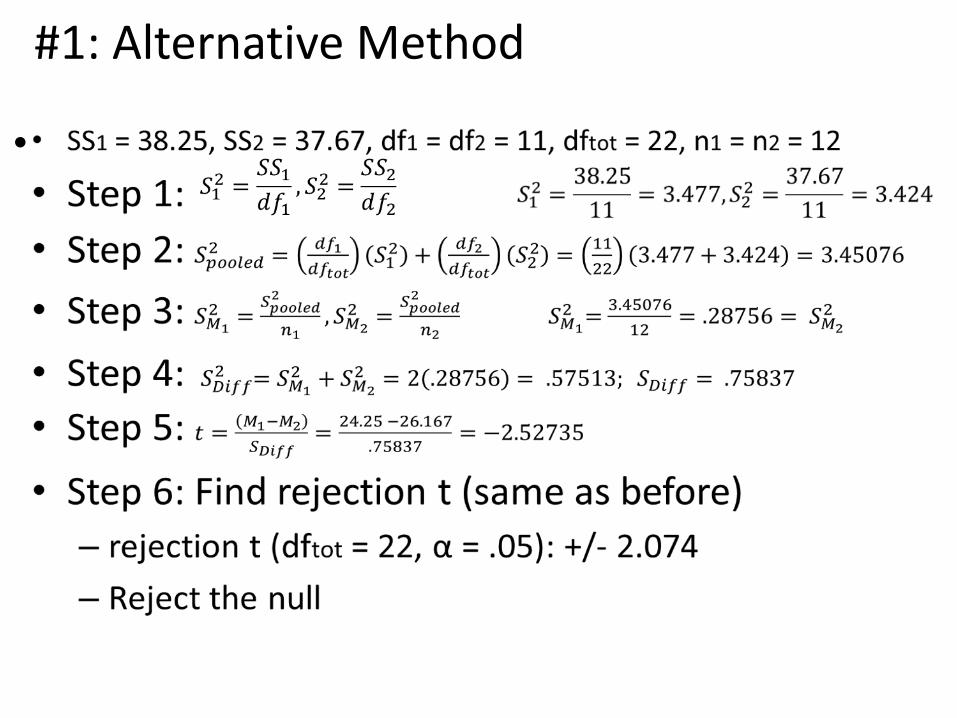
#1: Alternative Method
•

#2: Correlation• Another investigator believes that introversion/extraversion has a linear relationship to spelling ability and reports the following data:
Introversion Spelling.21 3114 3313 3913 2420 3521 3711 3615 2023 4612 3117 4426 44

#2: 201 Method: Calculating the Pearson Correlation (r)
Where n = the number of cases ΣXY = the sum of X values x Y values ΣX = the sum of x values ΣY = the sum of Y values
To determine CV, find df = np- 2, then use the table on slide 9.
[ ][ ]2222 )()( YYnXXnYXXYnr
Σ−ΣΣ−Σ
ΣΣ−Σ=

#2: 201 MethodIntroversion*(X) Spelling*(Y) X*Y X^2 Y^2
21 31 651 441 96114 33 462 196 108913 39 507 169 152113 24 312 169 57620 35 700 400 122521 37 777 441 136911 36 396 121 129615 20 300 225 40023 46 1058 529 211612 31 372 144 96117 44 748 289 193626 44 1144 676 1936206 420 7427 3800 15386 Sums
nΣXY = 12(7427) = 89124 ΣXΣY = 206(420) = 86520 nΣ(X^2) = 12(3800) = 45600 (ΣX)^2 = (206)^2 = 42436 nΣ(Y^2) = 12(15386) = 184362 (ΣY)^2 = (420)^2 = 176400
[ ][ ]2222 )()( YYnXXnYXXYnr
Σ−ΣΣ−Σ
ΣΣ−Σ=
CV: df = 12 – 2 = 10
Rejection r:
For α = .05, it’s r = .5760 (see next slide).
Fail to reject the null:
.5102 < .5760
[ ][ ]17640018436242436456008652089124
−−
−=r
[ ][ ]5102.
53.51032604
823231642604
===r

This is similar to the table in some 201
textbooks (Glenberg & Andrzejewski,
“Learning from Data,” p. 540)
#2: 201 Method, continued

#2: Alternative Method•
Introversion*(X) Dev.X Sq.Dev.X Spelling*(Y) Dev.Y Sq.Dev.Y Dev.X*Dev.Y21 3.833 14.6944 31 >4 16 >15.333333314 >3.17 10.0278 33 >2 4 6.33333333313 >4.17 17.3611 39 4 16 >16.666666713 >4.17 17.3611 24 >11 121 45.8333333320 2.833 8.02778 35 0 0 021 3.833 14.6944 37 2 4 7.66666666711 >6.17 38.0278 36 1 1 >6.1666666715 >2.17 4.69444 20 >15 225 32.523 5.833 34.0278 46 11 121 64.1666666712 >5.17 26.6944 31 >4 16 20.6666666717 >0.17 0.02778 44 9 81 >1.526 8.833 78.0278 44 9 81 79.5206 263.667 420 686 217 Sums
17.16666667 35 Means
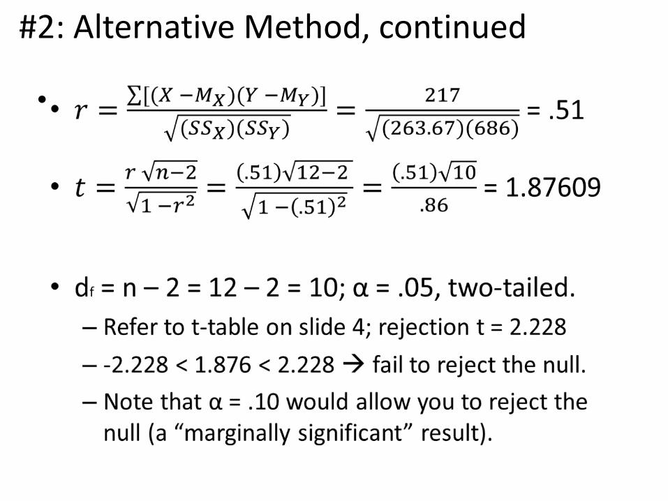
#2: Alternative Method, continued
•
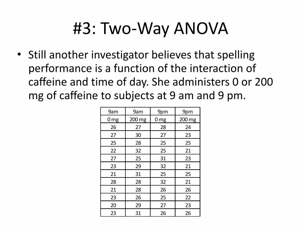
#3: Two-‐Way ANOVA• Still another investigator believes that spelling performance is a function of the interaction of caffeine and time of day. She administers 0 or 200 mg of caffeine to subjects at 9 am and 9 pm.
9am 9am 9pm 9pm0&mg 200&mg 0&mg&&&& 200&mg26 27 28 2427 30 27 2325 28 25 2522 32 25 2127 25 31 2323 29 32 2121 31 25 2528 28 32 2121 28 26 2623 26 25 2220 29 27 2323 31 26 26

#3: Alternative Method (for 2 x 2 ANOVA)*•

#3: Alternative Method (Ugly, but True)
• See next slide for means used here…
Morning'(9'am) Evening'(9'pm)0'mg X X3GM (X'3'GM)^2 X3M (X3M)^2 (Mr'3'GM)^2 (Mc'3'GM)^2 INT* INT^2 X X3GM (X'3'GM)^2 X3M (X3M)^2 (Mr'3'GM)^2 (Mc'3'GM)^2 INT* INT^2
26 0.188 0.0351563 2.167 4.69444 0.03515625 0.19140625 32.2 4.969 28 2.188 4.7851563 0.583 0.34028 0.03515625 0.19140625 2.23 4.96927 1.188 1.4101563 3.167 10.0278 0.03515625 0.19140625 32.2 4.969 27 1.188 1.4101563 30.42 0.17361 0.03515625 0.19140625 2.23 4.96925 30.813 0.6601563 1.167 1.36111 0.03515625 0.19140625 32.2 4.969 25 30.81 0.6601563 32.42 5.84028 0.03515625 0.19140625 2.23 4.96922 33.813 14.535156 31.83 3.36111 0.03515625 0.19140625 32.2 4.969 25 30.81 0.6601563 32.42 5.84028 0.03515625 0.19140625 2.23 4.96927 1.188 1.4101563 3.167 10.0278 0.03515625 0.19140625 32.2 4.969 31 5.188 26.910156 3.583 12.8403 0.03515625 0.19140625 2.23 4.96923 32.813 7.9101563 30.83 0.69444 0.03515625 0.19140625 32.2 4.969 32 6.188 38.285156 4.583 21.0069 0.03515625 0.19140625 2.23 4.96921 34.813 23.160156 32.83 8.02778 0.03515625 0.19140625 32.2 4.969 25 30.81 0.6601563 32.42 5.84028 0.03515625 0.19140625 2.23 4.96928 2.188 4.7851563 4.167 17.3611 0.03515625 0.19140625 32.2 4.969 32 6.188 38.285156 4.583 21.0069 0.03515625 0.19140625 2.23 4.96921 34.813 23.160156 32.83 8.02778 0.03515625 0.19140625 32.2 4.969 26 0.188 0.0351563 31.42 2.00694 0.03515625 0.19140625 2.23 4.96923 32.813 7.9101563 30.83 0.69444 0.03515625 0.19140625 32.2 4.969 25 30.81 0.6601563 32.42 5.84028 0.03515625 0.19140625 2.23 4.96920 35.813 33.785156 33.83 14.6944 0.03515625 0.19140625 32.2 4.969 27 1.188 1.4101563 30.42 0.17361 0.03515625 0.19140625 2.23 4.96923 32.813 7.9101563 30.83 0.69444 0.03515625 0.19140625 32.2 4.969 26 0.188 0.0351563 31.42 2.00694 0.03515625 0.19140625 2.23 4.969
Sums 286 126.67188 79.6667 0.421875 2.296875 59.63 329 113.79688 82.9167 0.421875 2.296875 59.63
200#mg X X'GM (X#'#GM)^2 X'M (X'M)^2 (Mr#'#GM)^2 (Mc#'#GM)^2 INT* INT^2 X X'GM (X#'#GM)^2 X'M (X'M)^2 (Mr#'#GM)^2 (Mc#'#GM)^2 INT* INT^227 1.188 1.4101563 '1.67 2.77778 0.03515625 0.19140625 2.23 4.969 24 '1.81 3.2851563 0.667 0.44444 0.03515625 0.19140625 '2.23 4.96930 4.188 17.535156 1.333 1.77778 0.03515625 0.19140625 2.23 4.969 23 '2.81 7.9101563 '0.33 0.11111 0.03515625 0.19140625 '2.23 4.96928 2.188 4.7851563 '0.67 0.44444 0.03515625 0.19140625 2.23 4.969 25 '0.81 0.6601563 1.667 2.77778 0.03515625 0.19140625 '2.23 4.96932 6.188 38.285156 3.333 11.1111 0.03515625 0.19140625 2.23 4.969 21 '4.81 23.160156 '2.33 5.44444 0.03515625 0.19140625 '2.23 4.96925 '0.813 0.6601563 '3.67 13.4444 0.03515625 0.19140625 2.23 4.969 23 '2.81 7.9101563 '0.33 0.11111 0.03515625 0.19140625 '2.23 4.96929 3.188 10.160156 0.333 0.11111 0.03515625 0.19140625 2.23 4.969 21 '4.81 23.160156 '2.33 5.44444 0.03515625 0.19140625 '2.23 4.96931 5.188 26.910156 2.333 5.44444 0.03515625 0.19140625 2.23 4.969 25 '0.81 0.6601563 1.667 2.77778 0.03515625 0.19140625 '2.23 4.96928 2.188 4.7851563 '0.67 0.44444 0.03515625 0.19140625 2.23 4.969 21 '4.81 23.160156 '2.33 5.44444 0.03515625 0.19140625 '2.23 4.96928 2.188 4.7851563 '0.67 0.44444 0.03515625 0.19140625 2.23 4.969 26 0.188 0.0351563 2.667 7.11111 0.03515625 0.19140625 '2.23 4.96926 0.188 0.0351563 '2.67 7.11111 0.03515625 0.19140625 2.23 4.969 22 '3.81 14.535156 '1.33 1.77778 0.03515625 0.19140625 '2.23 4.96929 3.188 10.160156 0.333 0.11111 0.03515625 0.19140625 2.23 4.969 23 '2.81 7.9101563 '0.33 0.11111 0.03515625 0.19140625 '2.23 4.96931 5.188 26.910156 2.333 5.44444 0.03515625 0.19140625 2.23 4.969 26 0.188 0.0351563 2.667 7.11111 0.03515625 0.19140625 '2.23 4.969
Sums 344 146.42188 48.6667 0.421875 2.296875 59.63 280 112.42188 38.6667 0.421875 2.296875 59.63

#3: Alternative Method•

#3: Sample F tableCritical Value for df (1,44) = 4.07 (approximately)
Note that you sometimes have to fudge a bit when estimating by hand—CV’s somewhere between 4.08 (df = 1, 40) and 4.00 (df = 1, 60) on this table.

#4: Chi-‐Square Test
• Another experimenter wants to test the hypothesis that gender is related to interest in football. 100 subjects (50 male and 50 female) are asked whether or not they watched a recent football game. The results are:
Watched(((( Did(not(watchMale 30 20Female 20 30
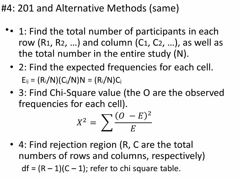
#4: 201 and Alternative Methods (same)
•

#4: 201 and Alternative Methods (same)• Watched(((( Did(not(watch Sums
Male O11(=(30 O12(=(20 R1(=(50Female O21(=(20 O22(=(30 R2(=(50Sums C1(=(50 C2(=(50 N(=(100

#4: Reject null if Chi-‐Square is equal to or greater than 3.841.
Sample Chi-‐Square Table
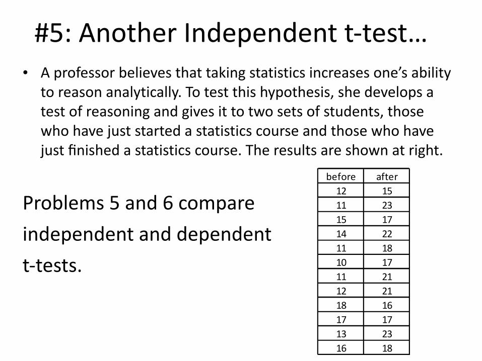
#5: Another Independent t-‐test…• A professor believes that taking statistics increases one’s ability
to reason analytically. To test this hypothesis, she develops a test of reasoning and gives it to two sets of students, those who have just started a statistics course and those who have just finished a statistics course. The results are shown at right.
Problems 5 and 6 compare independent and dependent t-‐tests.
before after12 1511 2315 1714 2211 1810 1711 2112 2118 1617 1713 2316 18

#5: 201 Method Only
Step 4: Rejection region
For α = .05, two-‐tailed, rejection t is (again) +/-‐ 2.074; since -‐5.07 < -‐.2.074, reject null
before&(G1) dev sq&dev after&(G2) dev sq&dev12 21.333 1.7778 15 24 1611 22.333 5.4444 23 4 1615 1.6667 2.7778 17 22 414 0.6667 0.4444 22 3 911 22.333 5.4444 18 21 110 23.333 11.111 17 22 411 22.333 5.4444 21 2 412 21.333 1.7778 21 2 418 4.6667 21.778 16 23 917 3.6667 13.444 17 22 413 20.333 0.1111 23 4 1616 2.6667 7.1111 18 21 1160 76.667 228 88 Sums
13.3333333 19 Meansdf1&=&df2&=&11
Step 1: Pooled variance
21
212
dfdfSSSSs p
+
+=
Step 2: Estimated Standard Error
2
2
1
2
21
ns
nss p
MMp+=−
Step 3: t-‐ statistic
21
21 )(MMsMMt
−
−=

#6: Dependent Samples t-‐test• Another professor has the same hypothesis, but decides to use a pre-‐post design. That is, each student takes the reasoning test twice, once before and once after the class. Results are the same as in #5: before after
12 1511 2315 1714 2211 1810 1711 2112 2118 1617 1713 2316 18
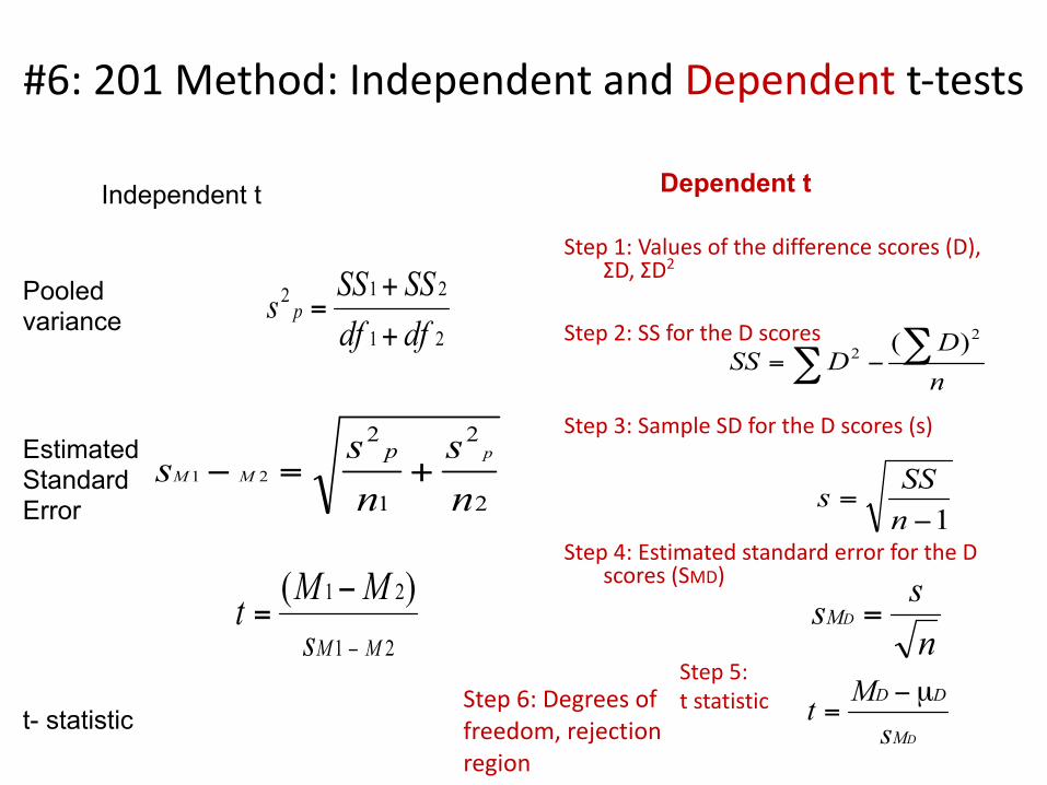
#6: 201 Method: Independent and Dependent t-‐tests
Step 1: Values of the difference scores (D), ΣD, ΣD2
Step 2: SS for the D scores
Step 3: Sample SD for the D scores (s)
Step 4: Estimated standard error for the D scores (SMD)
Step 5: t statistic
1−=nSSs
nss DM =
∑ ∑−=nD
DSS2
2 )(21
212
dfdfSSSSs p
+
+=
21
21 )(MMsMMt
−
−=
Pooled variance
Estimated Standard Error
t- statistic
2
2
1
2
21
ns
nss p
MMp+=−
DM
DD
sMt µ−
=
Independent t Dependent t
Step 6: Degrees of freedom, rejection region

#6: 201 MethodStep 1: Values of the difference scores (D), ΣD, ΣD2 :
Step 2: SS for the D scores:
before after D D^212 15 3 911 23 12 14415 17 2 414 22 8 6411 18 7 4910 17 7 4911 21 10 10012 21 9 8118 16 42 417 17 0 013 23 10 10016 18 2 4
Sums 160 228 68 608Means 13.333 19 5.7 50.6667n<=<12 D<=<after<4<before.
∑ ∑−=nD
DSS2
2 )(
Step 3: Sample SD for the D scores (s)
1−=nSSs
Step 4: Estimated standard error for the D scores (SMD)
nss DM =
Step 5: t statistic
DM
DD
sMt µ−
=
Step 6: Degrees of freedom, rejection regiondf#=#12#'#1#=#11For#p#<#.05#and#two#tails…t#>#2.201#ort#<#'2.201Since#4.363#>#2.201,#reject#null.

#6: Alternative MethodStep 1: Slightly different way of finding SS = 222.67. Step 2: Modified version of 201 method, step 3 Find sample variance of the D scores:
Step 3: Modified version of 201 method, step 4 Find estimated variance of the D scores:
Step 4: Find estimated standard deviation of the D scores (result same as in 201 method Step 4):
Step 5: Find t-‐statistic and rejection region (same as in 201 method): t = 4.363 Rejection t is 2.201 for p = .05, non-‐directional test 4.363 > 2.201; reject the null.
before after D D)*)M (D*M)^212 15 3 *2.7 7.1111111 23 12 6.33 40.111115 17 2 *3.7 13.444414 22 8 2.33 5.4444411 18 7 1.33 1.7777810 17 7 1.33 1.7777811 21 10 4.33 18.777812 21 9 3.33 11.111118 16 *2 *7.7 58.777817 17 0 *5.7 32.111113 23 10 4.33 18.777816 18 2 *3.7 13.4444
Sums 160 228 68 222.667Means M)= 5.667Difference)(D))=)after)*)before

#6: Independent v. Dependent t’s• Similarities between the two types:
– Population variance is unknown. – Population mean is unknown.
• Use in different situations: – Independent: Each participant has one score; compare mean of one group’s scores w/that of another.
– Dependent: Each participant has two scores; compare the pairs of scores to see if there’s a difference.
• Advantages of dependent t: – Uses same subjects in all treatment conditions
• No risk that subjects in one condition are substantially different from subjects in another; dependent t can be good when individual differences are expected to be substantial.
– Often more powerful than independent t • Disadvantages of dependent t:
– Carryover effects

#7a: The Normal Distribution
If a test is normally distributed and has a mean of 100 and a standard deviation of 15, then what percentage of students would you expect to have scores of 100 or greater?
SCORE
-4 -2 0 2 4
0.0
0.1
0.2
0.3
0.4
34%
14%
2%
Answer: 50%
Mean = 100

#7b: Z-‐scores and Z-‐tests
• If a test is normally distributed and has a mean of 100 and a standard deviation of 15, what percentage of students would you expect to have scores greater than 115?
…sometimes given as
…now look up Z = 1 on a Z table (or use graphic on previous slide)…
σ
µ)( −= i
iXZ

Sample Z table
Be careful to read your Z table’s instructions; some give percent under curve to the left of the Z score (scores below) and others give percent to the right (scores above); this one gives scores BELOW, so… Proportion w/Z scores greater than Z = 1 is 1 - .8413 = .1587, or 15.87% (about 16%, as shown in Slide 29 graphic)

#8: Probability
• If you flip a fair coin 10 times, how often would you expect to observe at least 8 heads?
• This is not the kind of problem that most introductory psych stats courses focus on.
• You might have covered this type of problem in other math courses (perhaps long ago).
• Still important, though—this kind of problem tends to crop up on standardized tests.

#8: Probability
• Denominator: Total number of possible outcomes of 10 fair coin flips – You can express these as length-‐10 vectors; e.g. THTTHTHHTT or TTTTTTTTTT.
• Numerator = Total number of possible outcomes of 10 fair coin flips with 8, 9, or 10 heads. – Easiest to deal with this as a sum w/three terms.
All outcomes of interest = (Combos w/10 heads) + (Combos w/9 heads) + (Combos w/8 heads) – Combos w/10 heads = 1 (only the HHHHHHHHHH combination has 10 heads) – Use the combination formula for Combos w/9 and Combos w/8 heads:
– Combos w/9 heads:
– Combos w/8 heads = 45 (similar calculation) • Answer to #8:
If you flip a fair coin 10 times, how often would you expect to observe at least 8 heads?

Guide to Bill’s Solutions • Detailed Syllabus, 9/28: “using R for statistics” pdf
– 1: Slides 25-‐45; solution on slide 34 (and 39) – 2: Slides 46-‐49; solution on slide 47 – 3: Slides 50-‐52; solution on slide 52
• Detailed Syllabus, 9/30: “stats homework solutions” pdf – 1: Solution on p.6 (“df = 21.999” means df = 22) – 2: Solution on p. 12 – 3: Solution on p. 14, p. 15 (drug = row, time = col) – 4: Solution on p.16 – 5: Solution on p.17 (“df = 21.896” means df = 22) – 6: Solution on p.17 – 7: Solution on p.18 – 8: Solution on p.20
• Moral #1: If you use R, there’s much less math that you have to do by hand…
• Moral #2: Excel junkies, there’s still hope—if you’re careful.


