Challenge H: For an even safer and more secure railway

1

Steady and moving high-speed train crosswind simulations. Comparisonwith wind-tunnel tests.

Federico Cheli, Daniele Rocchi, Paolo Schito, Gisella TomasiniDipartimento di Meccanica del Politecnico di Milano, via La Masa 1, 20156 Milano, Italy

Abstract

CFD simulations are used to investigate the effect of the relative motion between train and infrastructurein order to capture the differences between performing wind tunnel tests with static or moving vehicle tomeasure aerodynamic coefficient. Two infrastructure scenarios are considered: a single track ballast andrail and a 6m high embankment. CFD simulations are performed in the same geometrical scale of windtunnel tests to allow a numerical validation against experimental data on still models, both in terms ofglobal aerodynamic coefficients and surface pressure distribution, while the considerations on the relativemotion effects will be drawn from the comparisons between numerical results obtained with moving andstill models simulations.

KeywordsCross wind, high speed trains, moving vehicle, CFD simulation, aerodynamic coefficients, surfacepressure distribution

Introduction

In the present paper, the results of a CFD analysis on the effects of the train-infrastructure relative motionon the aerodynamic coefficients will be presented and discussed.The interest in such activity is related to the common practice, adopted in train aerodynamics studies, toperform wind tunnel tests on still models, reproducing the relative wind angle of attack in the horizontalplane by rotating both the train and the infrastructure models around the vertical axis.This situation is different from real one where the relative wind speed on the vehicle is due to the sum ofthe vectors of the train velocity and of the cross wind velocity, while the infrastructure, being still, issubjected to the absolute wind speed.In case of cross wind blowing perpendicular to the line, the infrastructure is actually run over by aperpendicular wind while the aerodynamic forces, acting on the train, are produced by the relative windthat is skewed in the horizontal plane.A scaled representation of the aerodynamic phenomena would require wind tunnel tests on movingmodels. The main drawbacks of this test methodology, relying on the experience of previous activities,performed also by the authors, are related to the test rig complexity, to the contemporary action ofaerodynamic and inertial forces and to the difficulty to keep a steady state condition for a long time [1] [2][3] [11].Considering high speed train applications (train speed higher than 250 km/h), the interesting wind-trainyaw angles are confined in a range between 0 and 30 deg (if cross wind speed higher than 25 m/s istaken into account). For still model tests the flow over the infrastructure is therefore far from the realcondition while for moving model tests this means that the train velocity vector represents the majorcontribution to the magnitude of the relative wind speed and the moving model in the wind tunnel has tomove faster than the wind speed. Among the major difficulties in performing moving vehicle tests themost demanding are: the need to perform many tests since only few seconds of steady state conditionsare available in each test run; and the need to deal with inertial forces and the dynamic behavior of themoving parts that may influence the train aerodynamics.In the authors’ experience, the comparison between experimental results on still and moving models iscomplicated by the uncertainties of all the mentioned aspects even if comparable results have been

Challenge H: For an even safer and more secure railway

1

Steady and moving high-speed train crosswind simulations. Comparisonwith wind-tunnel tests.

Federico Cheli, Daniele Rocchi, Paolo Schito, Gisella TomasiniDipartimento di Meccanica del Politecnico di Milano, via La Masa 1, 20156 Milano, Italy

Abstract

CFD simulations are used to investigate the effect of the relative motion between train and infrastructurein order to capture the differences between performing wind tunnel tests with static or moving vehicle tomeasure aerodynamic coefficient. Two infrastructure scenarios are considered: a single track ballast andrail and a 6m high embankment. CFD simulations are performed in the same geometrical scale of windtunnel tests to allow a numerical validation against experimental data on still models, both in terms ofglobal aerodynamic coefficients and surface pressure distribution, while the considerations on the relativemotion effects will be drawn from the comparisons between numerical results obtained with moving andstill models simulations.

KeywordsCross wind, high speed trains, moving vehicle, CFD simulation, aerodynamic coefficients, surfacepressure distribution

Introduction

In the present paper, the results of a CFD analysis on the effects of the train-infrastructure relative motionon the aerodynamic coefficients will be presented and discussed.The interest in such activity is related to the common practice, adopted in train aerodynamics studies, toperform wind tunnel tests on still models, reproducing the relative wind angle of attack in the horizontalplane by rotating both the train and the infrastructure models around the vertical axis.This situation is different from real one where the relative wind speed on the vehicle is due to the sum ofthe vectors of the train velocity and of the cross wind velocity, while the infrastructure, being still, issubjected to the absolute wind speed.In case of cross wind blowing perpendicular to the line, the infrastructure is actually run over by aperpendicular wind while the aerodynamic forces, acting on the train, are produced by the relative windthat is skewed in the horizontal plane.A scaled representation of the aerodynamic phenomena would require wind tunnel tests on movingmodels. The main drawbacks of this test methodology, relying on the experience of previous activities,performed also by the authors, are related to the test rig complexity, to the contemporary action ofaerodynamic and inertial forces and to the difficulty to keep a steady state condition for a long time [1] [2][3] [11].Considering high speed train applications (train speed higher than 250 km/h), the interesting wind-trainyaw angles are confined in a range between 0 and 30 deg (if cross wind speed higher than 25 m/s istaken into account). For still model tests the flow over the infrastructure is therefore far from the realcondition while for moving model tests this means that the train velocity vector represents the majorcontribution to the magnitude of the relative wind speed and the moving model in the wind tunnel has tomove faster than the wind speed. Among the major difficulties in performing moving vehicle tests themost demanding are: the need to perform many tests since only few seconds of steady state conditionsare available in each test run; and the need to deal with inertial forces and the dynamic behavior of themoving parts that may influence the train aerodynamics.In the authors’ experience, the comparison between experimental results on still and moving models iscomplicated by the uncertainties of all the mentioned aspects even if comparable results have been

Challenge H: For an even safer and more secure railway

1

Steady and moving high-speed train crosswind simulations. Comparisonwith wind-tunnel tests.

Federico Cheli, Daniele Rocchi, Paolo Schito, Gisella TomasiniDipartimento di Meccanica del Politecnico di Milano, via La Masa 1, 20156 Milano, Italy

Abstract

CFD simulations are used to investigate the effect of the relative motion between train and infrastructurein order to capture the differences between performing wind tunnel tests with static or moving vehicle tomeasure aerodynamic coefficient. Two infrastructure scenarios are considered: a single track ballast andrail and a 6m high embankment. CFD simulations are performed in the same geometrical scale of windtunnel tests to allow a numerical validation against experimental data on still models, both in terms ofglobal aerodynamic coefficients and surface pressure distribution, while the considerations on the relativemotion effects will be drawn from the comparisons between numerical results obtained with moving andstill models simulations.

KeywordsCross wind, high speed trains, moving vehicle, CFD simulation, aerodynamic coefficients, surfacepressure distribution

Introduction

In the present paper, the results of a CFD analysis on the effects of the train-infrastructure relative motionon the aerodynamic coefficients will be presented and discussed.The interest in such activity is related to the common practice, adopted in train aerodynamics studies, toperform wind tunnel tests on still models, reproducing the relative wind angle of attack in the horizontalplane by rotating both the train and the infrastructure models around the vertical axis.This situation is different from real one where the relative wind speed on the vehicle is due to the sum ofthe vectors of the train velocity and of the cross wind velocity, while the infrastructure, being still, issubjected to the absolute wind speed.In case of cross wind blowing perpendicular to the line, the infrastructure is actually run over by aperpendicular wind while the aerodynamic forces, acting on the train, are produced by the relative windthat is skewed in the horizontal plane.A scaled representation of the aerodynamic phenomena would require wind tunnel tests on movingmodels. The main drawbacks of this test methodology, relying on the experience of previous activities,performed also by the authors, are related to the test rig complexity, to the contemporary action ofaerodynamic and inertial forces and to the difficulty to keep a steady state condition for a long time [1] [2][3] [11].Considering high speed train applications (train speed higher than 250 km/h), the interesting wind-trainyaw angles are confined in a range between 0 and 30 deg (if cross wind speed higher than 25 m/s istaken into account). For still model tests the flow over the infrastructure is therefore far from the realcondition while for moving model tests this means that the train velocity vector represents the majorcontribution to the magnitude of the relative wind speed and the moving model in the wind tunnel has tomove faster than the wind speed. Among the major difficulties in performing moving vehicle tests themost demanding are: the need to perform many tests since only few seconds of steady state conditionsare available in each test run; and the need to deal with inertial forces and the dynamic behavior of themoving parts that may influence the train aerodynamics.In the authors’ experience, the comparison between experimental results on still and moving models iscomplicated by the uncertainties of all the mentioned aspects even if comparable results have been

Challenge H: For an even safer and more secure railway

2

obtained [3]. In the present study, CFD simulations have been performed to investigate how much theaerodynamic coefficient are modified by the relative motion between the train and the infrastructure.Numerical simulations are used as virtual experimental laboratory tests where the scaled model and theflow conditions are under control while the vehicle motion represents a simple change in the boundaryconditions [10].At the beginning, the same scaled testing conditions used in wind tunnel on still model have beenreproduced to validate the CFD approach. Two infrastructure scenarios have been considered: a smallerone where just a single track with ballast and rails is modeled and a larger one where a full double track 6m embankment is taken into account. They have been chosen since they are widely studied ([4], [5], [6])because they represent two of the configurations considered in European standards [7] and technicalspecifications [8] on cross wind effects on trains and overall they represent two situations where theinfrastructure plays a small and largerulein the whole models geometry. Infrastructure scenarios withinfinite length are considered in the CFD simulations by extruding the infrastructure geometry up to thenumerical domain in order to investigate just the relative motion effects while during wind tunnel tests afinite length infrastructure is used [3].After the initial validation of the numerical results comparing the aerodynamic coefficients and the surfacepressure distribution for different yaw angles on the still model with experimental results, CFD simulationshave been used to perform moving train tests using the same mesh and simulation set-up with a movingreference frame approach [10]. Numerical results have been therefore compared and considerationshave been proposed in the conclusions.

Model Setup

The analysis has been conducted on a 1:15 scaled model of an ETR500 train. The numerical setup hasbeen prepared in order to be representative of the experimental wind tunnel test performed at thePolitecnico di Milano Wind Tunnel [3]. The same CAD model that was used for the CNC machining of thewind tunnel modelis used to preparethe CFD mesh domain (Figure 2-a). The train convoy is made by afirst vehicle that was instrumented for the wind tunnel tests with a six components balance to measure theforces and moments, and by a second vehicle, reproducing a part of a trailer car to correctly reproducethe boundary condition for the flow around the leading car. Surface pressure distribution was measuredduring wind tunnel tests on STBR scenario using 156 pressure taps distributed over 24 sections on thefirst vehicle, according to the scheme reported in Figure 2-c.Forces, moments and pressures are reported in non-dimensional form as coefficients, calculatedaccording to the reference system of Figure 1-d as follows:

2 2 2

, ,1 1 12 2 2

i iP Fi Mi

F MpC C C i x y z

V V A V Ah

wherep is the static pressure, Fi is the force projected along the i-th direction, Mi the moment measuredaround the i-th axis with respect to the point located on the plane on the top of the rails in the middle ofthe rails and the boogies, ρ the air density, V the relative wind speed, A the train reference area (A=10m2

full-scale) and h is the train reference height (h=3m full-scale).

Figure 1: Single Track Ballast and Rail (STBR) scenario (left) and Double Track Ballast and Rail scenario on a CEN six meters highEmbankment (EMBK) on the right.

Challenge H: For an even safer and more secure railway

2

obtained [3]. In the present study, CFD simulations have been performed to investigate how much theaerodynamic coefficient are modified by the relative motion between the train and the infrastructure.Numerical simulations are used as virtual experimental laboratory tests where the scaled model and theflow conditions are under control while the vehicle motion represents a simple change in the boundaryconditions [10].At the beginning, the same scaled testing conditions used in wind tunnel on still model have beenreproduced to validate the CFD approach. Two infrastructure scenarios have been considered: a smallerone where just a single track with ballast and rails is modeled and a larger one where a full double track 6m embankment is taken into account. They have been chosen since they are widely studied ([4], [5], [6])because they represent two of the configurations considered in European standards [7] and technicalspecifications [8] on cross wind effects on trains and overall they represent two situations where theinfrastructure plays a small and largerulein the whole models geometry. Infrastructure scenarios withinfinite length are considered in the CFD simulations by extruding the infrastructure geometry up to thenumerical domain in order to investigate just the relative motion effects while during wind tunnel tests afinite length infrastructure is used [3].After the initial validation of the numerical results comparing the aerodynamic coefficients and the surfacepressure distribution for different yaw angles on the still model with experimental results, CFD simulationshave been used to perform moving train tests using the same mesh and simulation set-up with a movingreference frame approach [10]. Numerical results have been therefore compared and considerationshave been proposed in the conclusions.

Model Setup

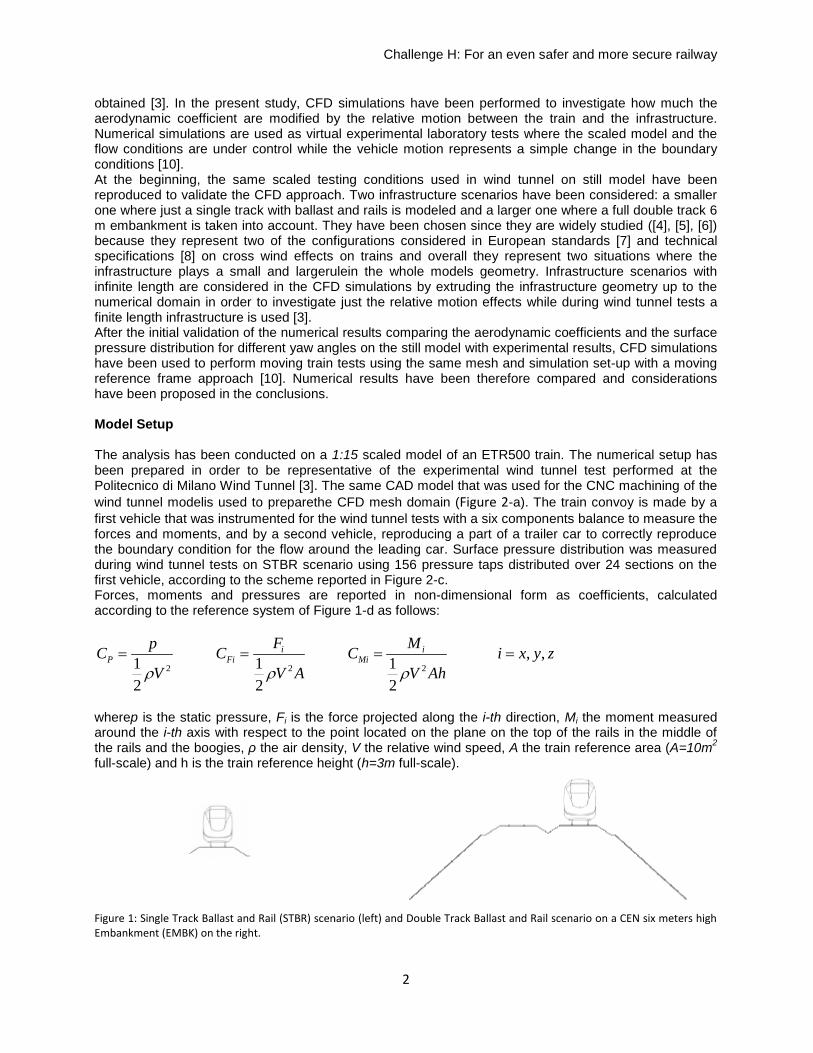
The analysis has been conducted on a 1:15 scaled model of an ETR500 train. The numerical setup hasbeen prepared in order to be representative of the experimental wind tunnel test performed at thePolitecnico di Milano Wind Tunnel [3]. The same CAD model that was used for the CNC machining of thewind tunnel modelis used to preparethe CFD mesh domain (Figure 2-a). The train convoy is made by afirst vehicle that was instrumented for the wind tunnel tests with a six components balance to measure theforces and moments, and by a second vehicle, reproducing a part of a trailer car to correctly reproducethe boundary condition for the flow around the leading car. Surface pressure distribution was measuredduring wind tunnel tests on STBR scenario using 156 pressure taps distributed over 24 sections on thefirst vehicle, according to the scheme reported in Figure 2-c.Forces, moments and pressures are reported in non-dimensional form as coefficients, calculatedaccording to the reference system of Figure 1-d as follows:

2 2 2

, ,1 1 12 2 2

i iP Fi Mi

F MpC C C i x y z

V V A V Ah

wherep is the static pressure, Fi is the force projected along the i-th direction, Mi the moment measuredaround the i-th axis with respect to the point located on the plane on the top of the rails in the middle ofthe rails and the boogies, ρ the air density, V the relative wind speed, A the train reference area (A=10m2

full-scale) and h is the train reference height (h=3m full-scale).

Figure 1: Single Track Ballast and Rail (STBR) scenario (left) and Double Track Ballast and Rail scenario on a CEN six meters highEmbankment (EMBK) on the right.

Challenge H: For an even safer and more secure railway

2

obtained [3]. In the present study, CFD simulations have been performed to investigate how much theaerodynamic coefficient are modified by the relative motion between the train and the infrastructure.Numerical simulations are used as virtual experimental laboratory tests where the scaled model and theflow conditions are under control while the vehicle motion represents a simple change in the boundaryconditions [10].At the beginning, the same scaled testing conditions used in wind tunnel on still model have beenreproduced to validate the CFD approach. Two infrastructure scenarios have been considered: a smallerone where just a single track with ballast and rails is modeled and a larger one where a full double track 6m embankment is taken into account. They have been chosen since they are widely studied ([4], [5], [6])because they represent two of the configurations considered in European standards [7] and technicalspecifications [8] on cross wind effects on trains and overall they represent two situations where theinfrastructure plays a small and largerulein the whole models geometry. Infrastructure scenarios withinfinite length are considered in the CFD simulations by extruding the infrastructure geometry up to thenumerical domain in order to investigate just the relative motion effects while during wind tunnel tests afinite length infrastructure is used [3].After the initial validation of the numerical results comparing the aerodynamic coefficients and the surfacepressure distribution for different yaw angles on the still model with experimental results, CFD simulationshave been used to perform moving train tests using the same mesh and simulation set-up with a movingreference frame approach [10]. Numerical results have been therefore compared and considerationshave been proposed in the conclusions.

Model Setup

The analysis has been conducted on a 1:15 scaled model of an ETR500 train. The numerical setup hasbeen prepared in order to be representative of the experimental wind tunnel test performed at thePolitecnico di Milano Wind Tunnel [3]. The same CAD model that was used for the CNC machining of thewind tunnel modelis used to preparethe CFD mesh domain (Figure 2-a). The train convoy is made by afirst vehicle that was instrumented for the wind tunnel tests with a six components balance to measure theforces and moments, and by a second vehicle, reproducing a part of a trailer car to correctly reproducethe boundary condition for the flow around the leading car. Surface pressure distribution was measuredduring wind tunnel tests on STBR scenario using 156 pressure taps distributed over 24 sections on thefirst vehicle, according to the scheme reported in Figure 2-c.Forces, moments and pressures are reported in non-dimensional form as coefficients, calculatedaccording to the reference system of Figure 1-d as follows:

2 2 2

, ,1 1 12 2 2

i iP Fi Mi

F MpC C C i x y z

V V A V Ah

wherep is the static pressure, Fi is the force projected along the i-th direction, Mi the moment measuredaround the i-th axis with respect to the point located on the plane on the top of the rails in the middle ofthe rails and the boogies, ρ the air density, V the relative wind speed, A the train reference area (A=10m2

full-scale) and h is the train reference height (h=3m full-scale).

Figure 1: Single Track Ballast and Rail (STBR) scenario (left) and Double Track Ballast and Rail scenario on a CEN six meters highEmbankment (EMBK) on the right.

Challenge H: For an even safer and more secure railway

3

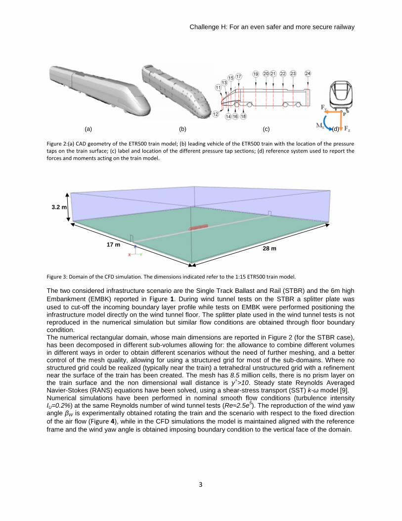
Figure 2:(a) CAD geometry of the ETR500 train model; (b) leading vehicle of the ETR500 train with the location of the pressuretaps on the train surface; (c) label and location of the different pressure tap sections; (d) reference system used to report theforces and moments acting on the train model.

Figure 3: Domain of the CFD simulation. The dimensions indicated refer to the 1:15 ETR500 train model.

The two considered infrastructure scenario are the Single Track Ballast and Rail (STBR) and the 6m highEmbankment (EMBK) reported in Figure 1. During wind tunnel tests on the STBR a splitter plate wasused to cut-off the incoming boundary layer profile while tests on EMBK were performed positioning theinfrastructure model directly on the wind tunnel floor. The splitter plate used in the wind tunnel tests is notreproduced in the numerical simulation but similar flow conditions are obtained through floor boundarycondition.The numerical rectangular domain, whose main dimensions are reported in Figure 2 (for the STBR case),has been decomposed in different sub-volumes allowing for: the allowance to combine different volumesin different ways in order to obtain different scenarios without the need of further meshing, and a bettercontrol of the mesh quality, allowing for using a structured grid for most of the sub-domains. Where nostructured grid could be realized (typically near the train) a tetrahedral unstructured grid with a refinementnear the surface of the train has been created. The mesh has 8.5 million cells, there is no prism layer onthe train surface and the non dimensional wall distance is y+>10. Steady state Reynolds AveragedNavier-Stokes (RANS) equations have been solved, using a shear-stress transport (SST) k-ω model [9].Numerical simulations have been performed in nominal smooth flow conditions (turbulence intensityIU=0.2%) at the same Reynolds number of wind tunnel tests (Re≈2.5e5). The reproduction of the wind yawangle βW is experimentally obtained rotating the train and the scenario with respect to the fixed directionof the air flow (Figure 4), while in the CFD simulations the model is maintained aligned with the referenceframe and the wind yaw angle is obtained imposing boundary condition to the vertical face of the domain.

3.2 m

17 m 28 m

(a) (b) (c) (d)

Challenge H: For an even safer and more secure railway

4

Figure 4: Reference for the relative wind incidence angle for both the STBR and the EMBK scenario.

CFD Validation

The comparison between experimental and CFD results are carried out in terms of forces and momentsacting on the first vehicle and on pressure distributions on the sections where the pressure taps arelocated. The analysis has been focused on wind incidence angles 0°<β<30°, because these angles aretypical of high speed trains.

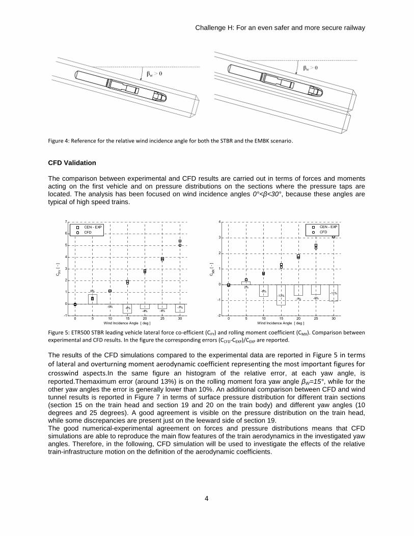
Figure 5: ETR500 STBR leading vehicle lateral force co-efficient (CFY) and rolling moment coefficient (CMX). Comparison betweenexperimental and CFD results. In the figure the corresponding errors (CCFD-CEXP)/CEXP are reported.

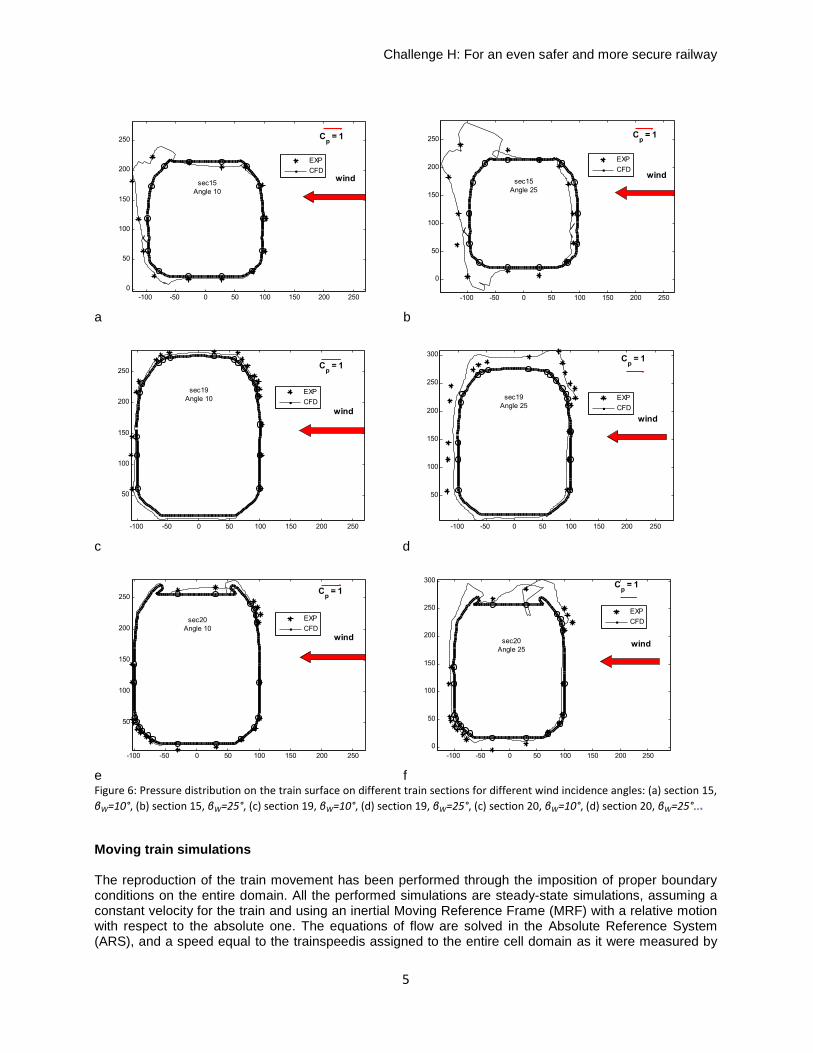
The results of the CFD simulations compared to the experimental data are reported in Figure 5 in termsof lateral and overturning moment aerodynamic coefficient representing the most important figures forcrosswind aspects.In the same figure an histogram of the relative error, at each yaw angle, isreported.Themaximum error (around 13%) is on the rolling moment fora yaw angle βW=15°, while for theother yaw angles the error is generally lower than 10%. An additional comparison between CFD and windtunnel results is reported in Figure 7 in terms of surface pressure distribution for different train sections(section 15 on the train head and section 19 and 20 on the train body) and different yaw angles (10degrees and 25 degrees). A good agreement is visible on the pressure distribution on the train head,while some discrepancies are present just on the leeward side of section 19.The good numerical-experimental agreement on forces and pressure distributions means that CFDsimulations are able to reproduce the main flow features of the train aerodynamics in the investigated yawangles. Therefore, in the following, CFD simulation will be used to investigate the effects of the relativetrain-infrastructure motion on the definition of the aerodynamic coefficients.

0 5 10 15 20 25 30-1

0

1

2

3

4

5

6

7

Wind Incidence Angle [ deg ]

CFY

[ - ]

8%

-0% -8%-4% -4%

-7%

CEN - EXPCFD

0 5 10 15 20 25 30-2

-1

0

1

2

3

4

Wind Incidence Angle [ deg ]

CM

X [ - ]

2%-8%

-13%-7% -6%

-11%

CEN - EXPCFD

Challenge H: For an even safer and more secure railway

5

a b

c d

e fFigure 6: Pressure distribution on the train surface on different train sections for different wind incidence angles: (a) section 15,βW=10°, (b) section 15, βW=25°, (c) section 19, βW=10°, (d) section 19, βW=25°, (c) section 20, βW=10°, (d) section 20, βW=25°...

Moving train simulations

The reproduction of the train movement has been performed through the imposition of proper boundaryconditions on the entire domain. All the performed simulations are steady-state simulations, assuming aconstant velocity for the train and using an inertial Moving Reference Frame (MRF) with a relative motionwith respect to the absolute one. The equations of flow are solved in the Absolute Reference System(ARS), and a speed equal to the trainspeedis assigned to the entire cell domain as it were measured by

-100 -50 0 50 100 150 200 2500

50

100

150

200

250

wind

Cp = 1

sec15Angle 10

EXPCFD

-100 -50 0 50 100 150 200 250

0

50

100

150

200

250

wind

Cp = 1

sec15Angle 25

EXPCFD

-100 -50 0 50 100 150 200 250

50

100

150

200

250

wind

Cp = 1

sec19Angle 10

EXPCFD

-100 -50 0 50 100 150 200 250

50

100

150

200

250

300

wind

Cp = 1

sec19Angle 25

EXPCFD

-100 -50 0 50 100 150 200 250

50

100

150

200

250

wind

Cp = 1

sec20Angle 10

EXPCFD

-100 -50 0 50 100 150 200 2500

50

100

150

200

250

300

wind

Cp = 1

sec20Angle 25

EXPCFD

Challenge H: For an even safer and more secure railway

6

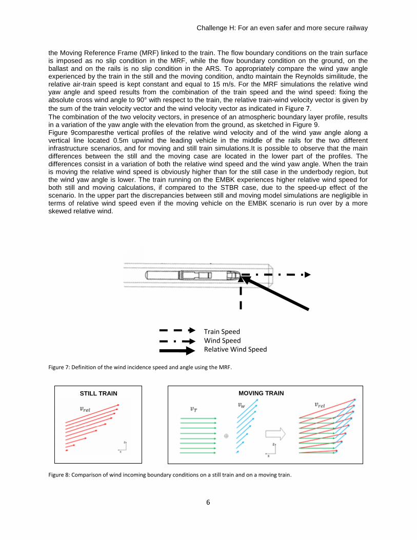
the Moving Reference Frame (MRF) linked to the train. The flow boundary conditions on the train surfaceis imposed as no slip condition in the MRF, while the flow boundary condition on the ground, on theballast and on the rails is no slip condition in the ARS. To appropriately compare the wind yaw angleexperienced by the train in the still and the moving condition, andto maintain the Reynolds similitude, therelative air-train speed is kept constant and equal to 15 m/s. For the MRF simulations the relative windyaw angle and speed results from the combination of the train speed and the wind speed: fixing theabsolute cross wind angle to 90° with respect to the train, the relative train-wind velocity vector is given bythe sum of the train velocity vector and the wind velocity vector as indicated in Figure 7.The combination of the two velocity vectors, in presence of an atmospheric boundary layer profile, resultsin a variation of the yaw angle with the elevation from the ground, as sketched in Figure 9.Figure 9comparesthe vertical profiles of the relative wind velocity and of the wind yaw angle along avertical line located 0.5m upwind the leading vehicle in the middle of the rails for the two differentinfrastructure scenarios, and for moving and still train simulations.It is possible to observe that the maindifferences between the still and the moving case are located in the lower part of the profiles. Thedifferences consist in a variation of both the relative wind speed and the wind yaw angle. When the trainis moving the relative wind speed is obviously higher than for the still case in the underbody region, butthe wind yaw angle is lower. The train running on the EMBK experiences higher relative wind speed forboth still and moving calculations, if compared to the STBR case, due to the speed-up effect of thescenario. In the upper part the discrepancies between still and moving model simulations are negligible interms of relative wind speed even if the moving vehicle on the EMBK scenario is run over by a moreskewed relative wind.

Figure 7: Definition of the wind incidence speed and angle using the MRF.

Figure 8: Comparison of wind incoming boundary conditions on a still train and on a moving train.

STILL TRAIN MOVING TRAIN

Train SpeedWind SpeedRelative Wind Speed

Challenge H: For an even safer and more secure railway

7

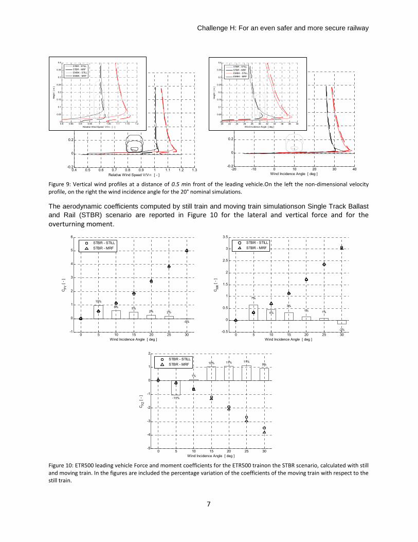
Figure 9: Vertical wind profiles at a distance of 0.5 min front of the leading vehicle.On the left the non-dimensional velocityprofile, on the right the wind incidence angle for the 20° nominal simulations.

The aerodynamic coefficients computed by still train and moving train simulationson Single Track Ballastand Rail (STBR) scenario are reported in Figure 10 for the lateral and vertical force and for theoverturning moment.

Figure 10: ETR500 leading vehicle Force and moment coefficients for the ETR500 trainon the STBR scenario, calculated with stilland moving train. In the figures are included the percentage variation of the coefficients of the moving train with respect to thestill train.

0 5 10 15 20 25 30-1

0

1

2

3

4

5

6

Wind Incidence Angle [ deg ]

CFY

[ - ]

10%

6% 5%2% 2%

-0%

STBR - STILLSTBR - MRF

0 5 10 15 20 25 30-0.5

0

0.5

1

1.5

2

2.5

3

3.5

Wind Incidence Angle [ deg ]

CM

X [ - ]

7%

4%

3%1% 1%

-2%

STBR - STILLSTBR - MRF

0 5 10 15 20 25 30-5

-4

-3

-2

-1

0

1

2

Wind Incidence Angle [ deg ]

CFZ

[ - ] -11%

1%

10% 11% 11%9%

STBR - STILLSTBR - MRF

0.4 0.5 0.6 0.7 0.8 0.9 1 1.1 1.2 1.3-0.2

0

0.2

0.4

0.6

0.8

1

1.2

Relative Wind Speed V/V [ - ]

Hei

ght

[ m ]

STBR - STILLSTBR - MRFEMBK - STILLEMBK - MRF

-20 -10 0 10 20 30 40-0.2

0

0.2

0.4

0.6

0.8

1

1.2

Wind Incidence Angle [ deg ]

Hei

ght

[ m ]

STBR - STILLSTBR - MRFEMBK - STILLEMBK - MRF

20 22 24 26 28 30 32 34 36 38 400

0.05

0.1

0.15

0.2

0.25

0.3

0.35

0.4

Wind Incidence Angle [ deg ]

Hei

ght

[ m ]

STBR - STILLSTBR - MRFEMBK - STILLEMBK - MRF

0.8 0.85 0.9 0.95 1 1.05 1.1 1.15 1.20

0.05

0.1

0.15

0.2

0.25

0.3

0.35

0.4

Relative Wind Speed V/V [ - ]

Hei

ght

[ m ]

STBR - STILLSTBR - MRFEMBK - STILLEMBK - MRF

Challenge H: For an even safer and more secure railway

8

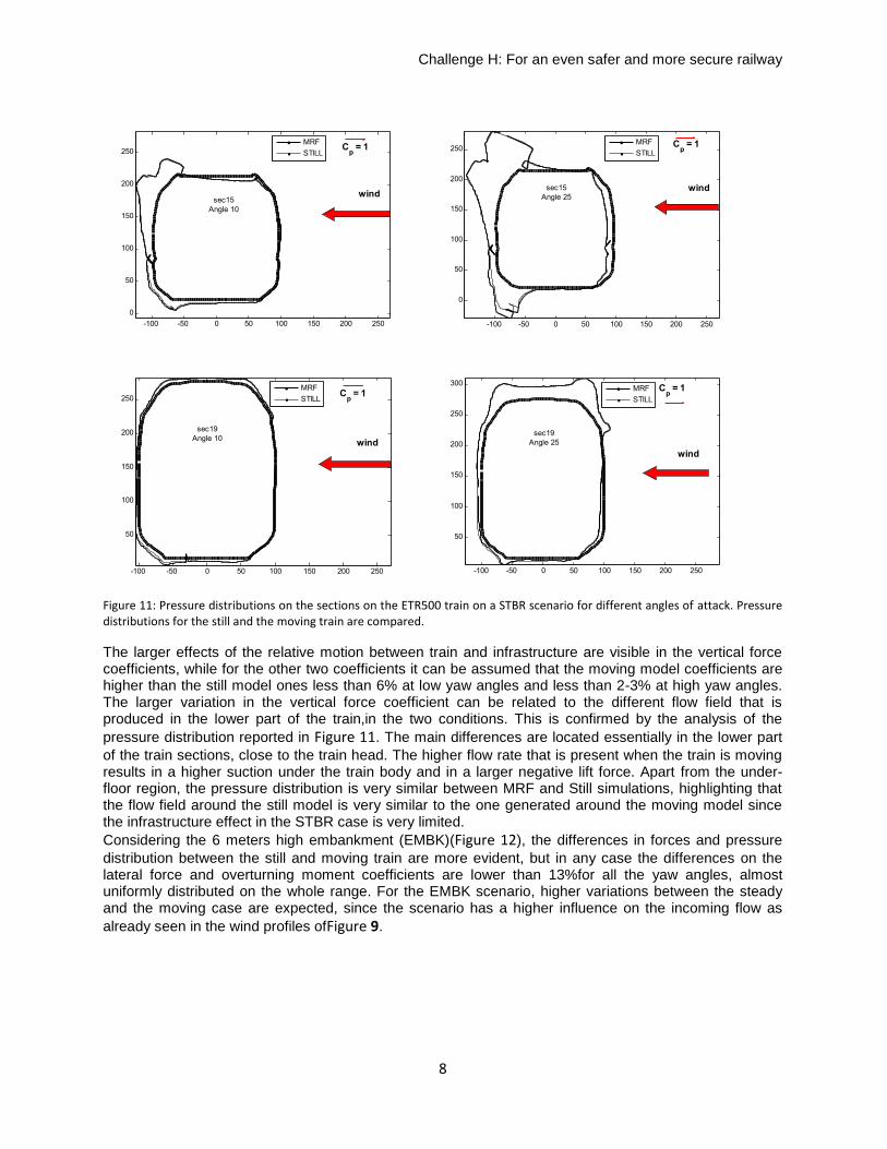
Figure 11: Pressure distributions on the sections on the ETR500 train on a STBR scenario for different angles of attack. Pressuredistributions for the still and the moving train are compared.

The larger effects of the relative motion between train and infrastructure are visible in the vertical forcecoefficients, while for the other two coefficients it can be assumed that the moving model coefficients arehigher than the still model ones less than 6% at low yaw angles and less than 2-3% at high yaw angles.The larger variation in the vertical force coefficient can be related to the different flow field that isproduced in the lower part of the train,in the two conditions. This is confirmed by the analysis of thepressure distribution reported in Figure 11. The main differences are located essentially in the lower partof the train sections, close to the train head. The higher flow rate that is present when the train is movingresults in a higher suction under the train body and in a larger negative lift force. Apart from the under-floor region, the pressure distribution is very similar between MRF and Still simulations, highlighting thatthe flow field around the still model is very similar to the one generated around the moving model sincethe infrastructure effect in the STBR case is very limited.Considering the 6 meters high embankment (EMBK)(Figure 12), the differences in forces and pressuredistribution between the still and moving train are more evident, but in any case the differences on thelateral force and overturning moment coefficients are lower than 13%for all the yaw angles, almostuniformly distributed on the whole range. For the EMBK scenario, higher variations between the steadyand the moving case are expected, since the scenario has a higher influence on the incoming flow asalready seen in the wind profiles ofFigure 9.

-100 -50 0 50 100 150 200 2500

50

100

150

200

250

wind

Cp = 1

sec15Angle 10

MRFSTILL

-100 -50 0 50 100 150 200 250

0

50

100

150

200

250

wind

Cp = 1

sec15Angle 25

MRFSTILL

-100 -50 0 50 100 150 200 250

50

100

150

200

250

wind

Cp = 1

sec19Angle 10

MRFSTILL

-100 -50 0 50 100 150 200 250

50

100

150

200

250

300

wind

Cp = 1

sec19Angle 25

MRFSTILL

Challenge H: For an even safer and more secure railway

9

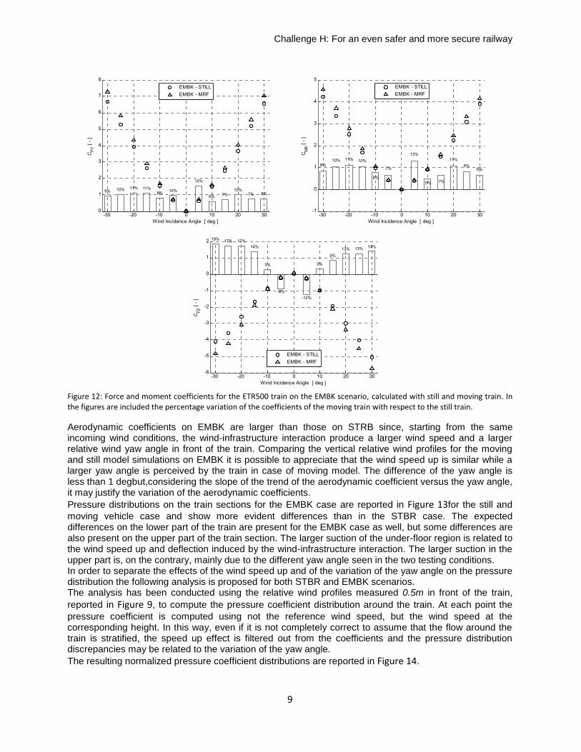
Figure 12: Force and moment coefficients for the ETR500 train on the EMBK scenario, calculated with still and moving train. Inthe figures are included the percentage variation of the coefficients of the moving train with respect to the still train.

Aerodynamic coefficients on EMBK are larger than those on STRB since, starting from the sameincoming wind conditions, the wind-infrastructure interaction produce a larger wind speed and a largerrelative wind yaw angle in front of the train. Comparing the vertical relative wind profiles for the movingand still model simulations on EMBK it is possible to appreciate that the wind speed up is similar while alarger yaw angle is perceived by the train in case of moving model. The difference of the yaw angle isless than 1 degbut,considering the slope of the trend of the aerodynamic coefficient versus the yaw angle,it may justify the variation of the aerodynamic coefficients.Pressure distributions on the train sections for the EMBK case are reported in Figure 13for the still andmoving vehicle case and show more evident differences than in the STBR case. The expecteddifferences on the lower part of the train are present for the EMBK case as well, but some differences arealso present on the upper part of the train section. The larger suction of the under-floor region is related tothe wind speed up and deflection induced by the wind-infrastructure interaction. The larger suction in theupper part is, on the contrary, mainly due to the different yaw angle seen in the two testing conditions.In order to separate the effects of the wind speed up and of the variation of the yaw angle on the pressuredistribution the following analysis is proposed for both STBR and EMBK scenarios.The analysis has been conducted using the relative wind profiles measured 0.5m in front of the train,reported in Figure 9, to compute the pressure coefficient distribution around the train. At each point thepressure coefficient is computed using not the reference wind speed, but the wind speed at thecorresponding height. In this way, even if it is not completely correct to assume that the flow around thetrain is stratified, the speed up effect is filtered out from the coefficients and the pressure distributiondiscrepancies may be related to the variation of the yaw angle.The resulting normalized pressure coefficient distributions are reported in Figure 14.

-30 -20 -10 0 10 20 300

1

2

3

4

5

6

7

8

Wind Incidence Angle [ deg ]

CFY

[ - ]

10%8%11%11%10%9%

1016%

15%

6% 7%10%

7% 8%

EMBK - STILLEMBK - MRF

-30 -20 -10 0 10 20 30-1

0

1

2

3

4

5

Wind Incidence Angle [ deg ]

CM

X [ - ]

7%

8%

10%11%10%8%

-1751%

13%

5% 7%

11%8%

6%

EMBK - STILLEMBK - MRF

-30 -20 -10 0 10 20 30-6

-5

-4

-3

-2

-1

0

1

2

Wind Incidence Angle [ deg ]

CFZ

[ - ]

-9%

3%

14%17%17%19%

130%

-12%

3%

9%13% 13% 14%

EMBK - STILLEMBK - MRF

Challenge H: For an even safer and more secure railway

10

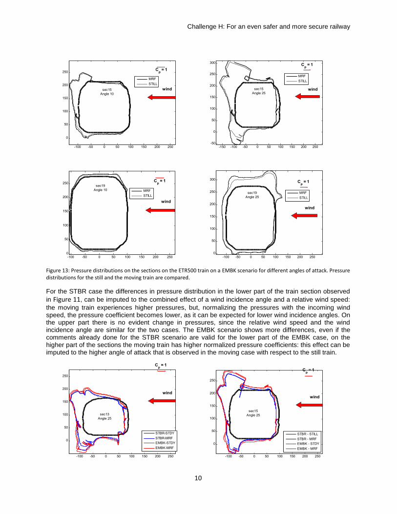
Figure 13: Pressure distributions on the sections on the ETR500 train on a EMBK scenario for different angles of attack. Pressuredistributions for the still and the moving train are compared.

For the STBR case the differences in pressure distribution in the lower part of the train section observedin Figure 11, can be imputed to the combined effect of a wind incidence angle and a relative wind speed:the moving train experiences higher pressures, but, normalizing the pressures with the incoming windspeed, the pressure coefficient becomes lower, as it can be expected for lower wind incidence angles. Onthe upper part there is no evident change in pressures, since the relative wind speed and the windincidence angle are similar for the two cases. The EMBK scenario shows more differences, even if thecomments already done for the STBR scenario are valid for the lower part of the EMBK case, on thehigher part of the sections the moving train has higher normalized pressure coefficients: this effect can beimputed to the higher angle of attack that is observed in the moving case with respect to the still train.

-100 -50 0 50 100 150 200 250

0

50

100

150

200

250

wind

Cp = 1

sec15Angle 10

MRFSTILL

-150 -100 -50 0 50 100 150 200 250-50

0

50

100

150

200

250

300

wind

Cp = 1

sec15Angle 25

MRFSTILL

-100 -50 0 50 100 150 200 2500

50

100

150

200

250

wind

Cp = 1sec19

Angle 10 MRFSTILL

-100 -50 0 50 100 150 200 2500

50

100

150

200

250

300

wind

Cp = 1

sec19Angle 25

MRFSTILL

-100 -50 0 50 100 150 200 250

0

50

100

150

200

250

wind

Cp = 1

sec13Angle 25

STBR-STDYSTBR-MRFEMBK-STDYEMBK-MRF

-100 -50 0 50 100 150 200 250

0

50

100

150

200

250

wind

Cp = 1

sec15Angle 25

STBR - STILLSTBR - MRFEMBK - STDYEMBK - MRF

Challenge H: For an even safer and more secure railway

11

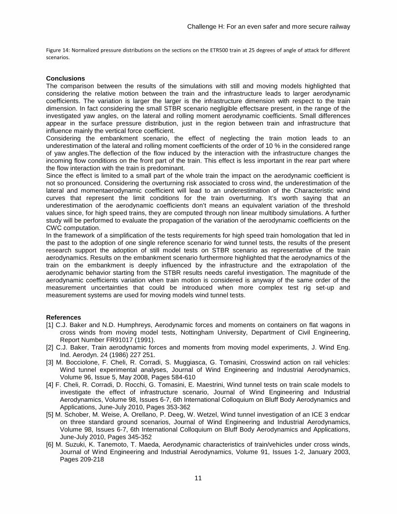
Figure 14: Normalized pressure distributions on the sections on the ETR500 train at 25 degrees of angle of attack for differentscenarios.

ConclusionsThe comparison between the results of the simulations with still and moving models highlighted thatconsidering the relative motion between the train and the infrastructure leads to larger aerodynamiccoefficients. The variation is larger the larger is the infrastructure dimension with respect to the traindimension. In fact considering the small STBR scenario negligible effectsare present, in the range of theinvestigated yaw angles, on the lateral and rolling moment aerodynamic coefficients. Small differencesappear in the surface pressure distribution, just in the region between train and infrastructure thatinfluence mainly the vertical force coefficient.Considering the embankment scenario, the effect of neglecting the train motion leads to anunderestimation of the lateral and rolling moment coefficients of the order of 10 % in the considered rangeof yaw angles.The deflection of the flow induced by the interaction with the infrastructure changes theincoming flow conditions on the front part of the train. This effect is less important in the rear part wherethe flow interaction with the train is predominant.Since the effect is limited to a small part of the whole train the impact on the aerodynamic coefficient isnot so pronounced. Considering the overturning risk associated to cross wind, the underestimation of thelateral and momentaerodynamic coefficient will lead to an underestimation of the Characteristic windcurves that represent the limit conditions for the train overturning. It’s worth saying that anunderestimation of the aerodynamic coefficients don’t means an equivalent variation of the thresholdvalues since, for high speed trains, they are computed through non linear multibody simulations. A furtherstudy will be performed to evaluate the propagation of the variation of the aerodynamic coefficients on theCWC computation.In the framework of a simplification of the tests requirements for high speed train homologation that led inthe past to the adoption of one single reference scenario for wind tunnel tests, the results of the presentresearch support the adoption of still model tests on STBR scenario as representative of the trainaerodynamics. Results on the embankment scenario furthermore highlighted that the aerodynamics of thetrain on the embankment is deeply influenced by the infrastructure and the extrapolation of theaerodynamic behavior starting from the STBR results needs careful investigation. The magnitude of theaerodynamic coefficients variation when train motion is considered is anyway of the same order of themeasurement uncertainties that could be introduced when more complex test rig set-up andmeasurement systems are used for moving models wind tunnel tests.

References[1] C.J. Baker and N.D. Humphreys, Aerodynamic forces and moments on containers on flat wagons in

cross winds from moving model tests, Nottingham University, Department of Civil Engineering,Report Number FR91017 (1991).

[2] C.J. Baker, Train aerodynamic forces and moments from moving model experiments, J. Wind Eng.Ind. Aerodyn. 24 (1986) 227 251.

[3] M. Bocciolone, F. Cheli, R. Corradi, S. Muggiasca, G. Tomasini, Crosswind action on rail vehicles:Wind tunnel experimental analyses, Journal of Wind Engineering and Industrial Aerodynamics,Volume 96, Issue 5, May 2008, Pages 584-610

[4] F. Cheli, R. Corradi, D. Rocchi, G. Tomasini, E. Maestrini, Wind tunnel tests on train scale models toinvestigate the effect of infrastructure scenario, Journal of Wind Engineering and IndustrialAerodynamics, Volume 98, Issues 6-7, 6th International Colloquium on Bluff Body Aerodynamics andApplications, June-July 2010, Pages 353-362

[5] M. Schober, M. Weise, A. Orellano, P. Deeg, W. Wetzel, Wind tunnel investigation of an ICE 3 endcaron three standard ground scenarios, Journal of Wind Engineering and Industrial Aerodynamics,Volume 98, Issues 6-7, 6th International Colloquium on Bluff Body Aerodynamics and Applications,June-July 2010, Pages 345-352

[6] M. Suzuki, K. Tanemoto, T. Maeda, Aerodynamic characteristics of train/vehicles under cross winds,Journal of Wind Engineering and Industrial Aerodynamics, Volume 91, Issues 1-2, January 2003,Pages 209-218

Challenge H: For an even safer and more secure railway

12

[7] CEN, 2010. EN 14067—railway applications aerodynamics—part 6: requirements and test proceduresfor cross wind assessment. European Norm, CEN/TC 256

[8] EC, 2006. TSI—Technical Specification for Interoperability of the trans-European high speed railsystem. European Law, Official Journal of the European Communities.

[9] F.R. Menter, Two-Equation Eddy-Viscosity Turbulence Models for Engineering Applications, AIAAJournal, 32(8):1598-1605, August 1994.

[10] C. Catanzaro, F. Cheli, D. Rocchi, P. Schito, G. Tomasini: “Hi-speed train crosswind analysis: CFDstudy and validation with wind-tunnel tests”, Proceedings of Aerodynamics of Heavy Vehicles III:Trucks, Buses and Trains, Potsdam, September 2010

[11] Li,Y.Hu,P.Zhang,M.,Liao,H.:Windtunneltestwithmovingvehiclemodelforaerody-namicforcesofvehicle-bridgesystemsundercrosswind.APCWE7TheSeventhAsia-PacificConferenceonWindEngineering,Taiwan,(2009)