62
Stellar Atmospheres: Emission and Absorption 1 Emission and Absorption
| Date post: | 22-Dec-2015 |
| Category: |
Documents |
| Upload: | rosamond-cunningham |
| View: | 239 times |
| Download: | 2 times |
Stellar Atmospheres: Emission and Absorption
1
Emission and Absorption
Stellar Atmospheres: Emission and Absorption
2
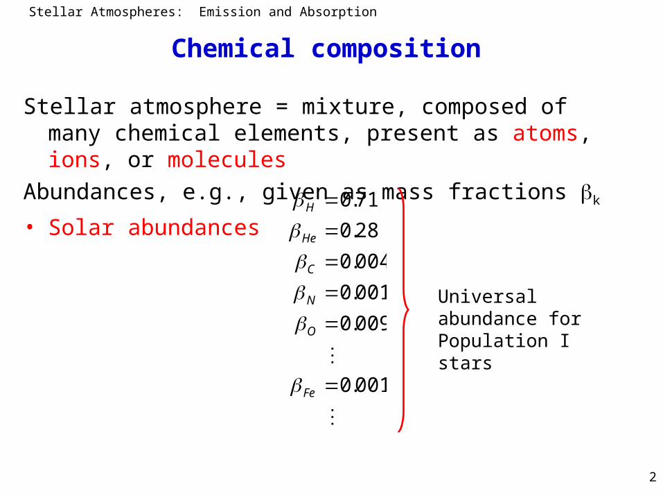
Chemical composition
Stellar atmosphere = mixture, composed of many chemical elements, present as atoms, ions, or molecules
Abundances, e.g., given as mass fractions k
• Solar abundances
001.0
009.0
001.0
004.0
28.0
71.0
Fe
O
N
C
He
H
Universal abundance for Population I stars

Stellar Atmospheres: Emission and Absorption
3
Chemical composition
• Population II stars
• Chemically peculiar stars,
e.g., helium stars
• Chemically peculiar stars,
e.g., PG1159 stars
0.1 0.00001
H H
He He
Z Z
¤
¤
¤
0.002
0.964
0.029
0.003
0.002
H H
He He
C C
N N
O O
¤
¤
¤
¤
¤
0.05
0.25
0.55
0.02
0.15
H H
He He
C C
N
O O
¤
¤
¤
¤
Stellar Atmospheres: Emission and Absorption
4
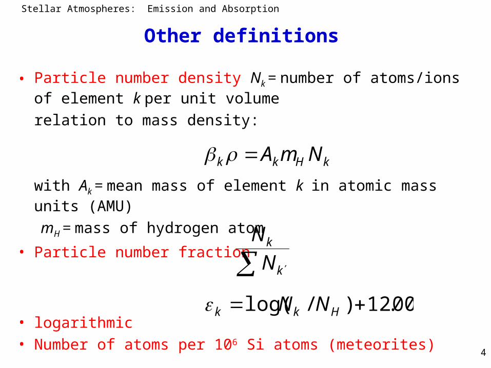
Other definitions
• Particle number density Nk = number of atoms/ions of element k per unit volume
relation to mass density:
with Ak = mean mass of element k in atomic mass units (AMU)
mH = mass of hydrogen atom
• Particle number fraction
• logarithmic• Number of atoms per 106 Si atoms (meteorites)
kHkk NmA
k
k
N
N
00.12)/log( Hkk NN
Stellar Atmospheres: Emission and Absorption
5
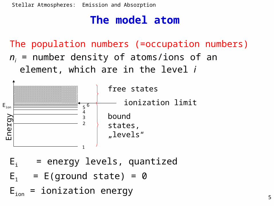
The model atom
The population numbers (=occupation numbers)
ni = number density of atoms/ions of an element, which are in the level i
Ei = energy levels, quantized
E1 = E(ground state) = 0
Eion = ionization energy
bound states, „levels“
free states
ionization limit
1
65432
En
erg
y
Eion
Stellar Atmospheres: Emission and Absorption
6
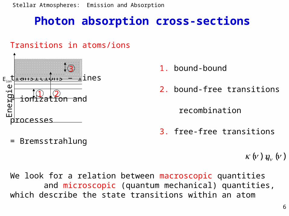
Transitions in atoms/ions
1. bound-bound transitions = lines
2. bound-free transitions = ionization and
recombination processes
3. free-free transitions = Bremsstrahlung
We look for a relation between macroscopic quantities and microscopic (quantum mechanical) quantities, which describe the state transitions within an atom
En
erg
ie
Eion
Photon absorption cross-sections
1 2
3
)(),(

Stellar Atmospheres: Emission and Absorption
7
Line transitions:Bound-free transitions: thermal average of electron velocities v(Maxwell distribution, i.e., electrons in thermodynamic equilibrium)
Free-free transition: free electron in Coulomb field of an ion, Bremsstrahlung, classically: jump into other hyperbolic orbit, arbitrary
For all processes holds: can only be supplied or removed by:– Inelastic collisions with other particles (mostly electrons), collisional
processes– By absorption/emission of a photon, radiative processes– In addition: scattering processes = (in)elastic collisions of photons with
electrons or atoms- scattering off free electrons: Thomson or Compton scattering- scattering off bound electrons: Rayleigh scattering
Photon absorption cross-sections
ffEE
2e
bf th ion low
unbound state ion free electron 1/ 2 m v
E E E E
lowupbb EEE
+
Stellar Atmospheres: Emission and Absorption
8
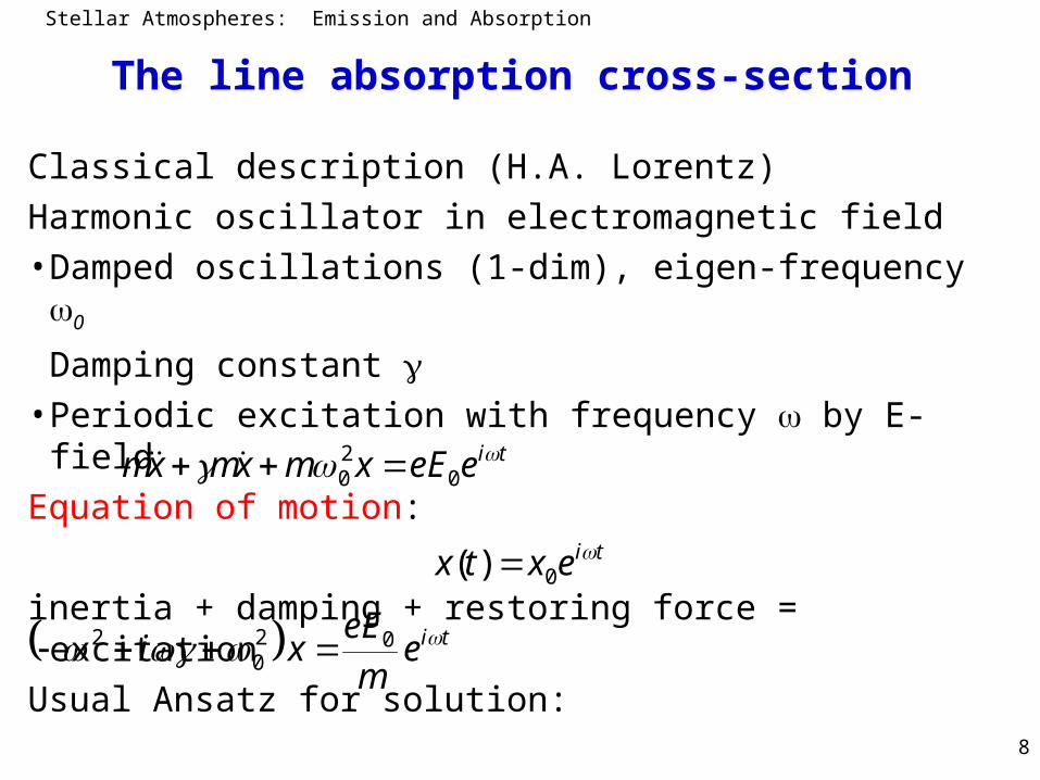
The line absorption cross-section
Classical description (H.A. Lorentz)
Harmonic oscillator in electromagnetic field
• Damped oscillations (1-dim), eigen-frequency 0
Damping constant • Periodic excitation with frequency by E-field
Equation of motion:
inertia + damping + restoring force = excitation
Usual Ansatz for solution:
tieeExmxmxm 020
tiextx 0)(
tiem
eExi 02
02
Stellar Atmospheres: Emission and Absorption
9
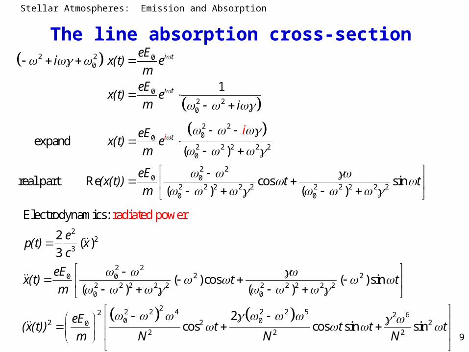
The line absorption cross-section
22
3
2 22 20 0
2 2 2 2 2 2 2 2 2 20 0
22 2 4 2 2 52 2 60 02 2 20
2 2 2
Electrodynamics:
2( )
3
( ) cos ( )sin( ) ( )
2cos co
radiated p
s sin s
ower
in
ep(t) x
c
eEx(t) t t
m
eE(x(t)) t t t t
m N N N
2 2 00
02 20
2 200
2 2 2 2 20
2 20 0
2 2 2 2 2 2 2 2 2 20 0
1
expand ( )
real part Re cos sin( ) ( )
i t
t
ti
i
eEi x(t) e
meE
x(t) em i
eEx(t) e
m
eE(x(t)) t t
i
m
Stellar Atmospheres: Emission and Absorption
10
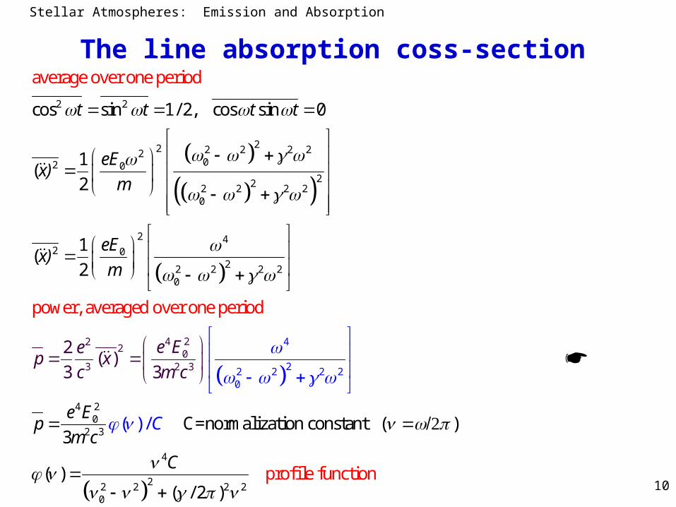
The line absorption coss-section
2 2
22 2 2 2 2202 0
222 2 2 20
2 42 0
22 2 2
2
0
3
2
average over one period
power, averaged ove
cos sin 1/ 2,
r one
cos sin 0
1(
2
1
perio
(2
3
d
2(
ep x
t t t t
eEx)
E)
m
c
m
ex
4 20
2
4 22
04
22 2 2 2
3
4
22 2 2
3
0
0
2
2
C=normalization constant ( )3
( ) profi
)3
le functi
( ) /
/
n( 2
o )
C
e
e Ep
m c
C
E
m c

Stellar Atmospheres: Emission and Absorption
11
The line absorption cross-section
0
0
0 0 0
2 2 2 2 2 20 0 0 0 0
2 20 0
2 2 2 20 0
0
since - , :
( ) (( )( )) 4 ( )
( )4( ) ( / 2 ) 4 ( ) ( / 4 )
now: calculating the normalization constant
( ) 1
4substitution: : ( )
(
C C
d
x
0
0
2 22 00 2 2 2
0
4)
4 1
=
C dxd C C
x
Stellar Atmospheres: Emission and Absorption
12
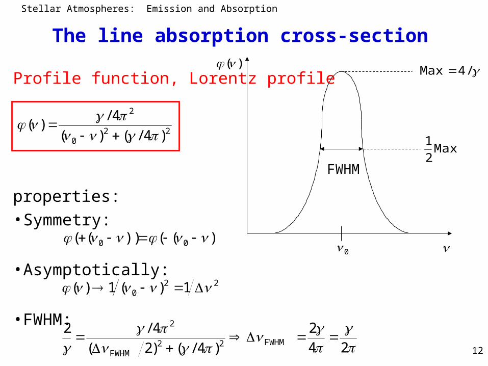
Profile function, Lorentz profile
properties:• Symmetry:
• Asymptotically:
• FWHM:
The line absorption cross-section
220
2
)4/()(
4/)(
/4Max
Max2
1
0
)(
FWHM
))(())(( 00
220 1)(1)(
24
2
)4/()2(
4/2FWHM22
FWHM
2

Stellar Atmospheres: Emission and Absorption
13
The damping constant
• Radiation damping, classically (other damping mechanisms later)
• Damping force (“friction“)
power=force velocity
electrodynamics
• Hence, Ansatz for frictional force is not correct• Help: define such, that the power is correct, when time-
averaged over one period:
classical radiation damping constant
)(txmF 2)()( txmtp
2
3
2
)(3
2)( tx
c
etp
22 4
03
2 (where we used ( ) )
3 i te
m x t x ec
3
20
2
0 3
2
mc
eωω
Stellar Atmospheres: Emission and Absorption
14
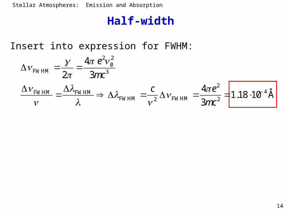
Half-width
Insert into expression for FWHM:2 2
0FWHM 3
24FWHM FWHM
FWHM FWHM2 2
4
2 3
41.18 10 Å
3
e
mc
c e
mc

Stellar Atmospheres: Emission and Absorption
15
The absorption cross-section
Definition absorption coefficient with nlow = number density of absorbers:
absorption cross-section (definition), dimension: area
Separating off frequency dependence:
Dimension : area frequency
Now: calculate absorption cross-section of classical harmonic oscillator for plane electromagnetic wave:
dsIdI )(low)()( n
)()()( 0
0
)1()(8
),( 20
0
Ec
I
eEE tix
Stellar Atmospheres: Emission and Absorption
16
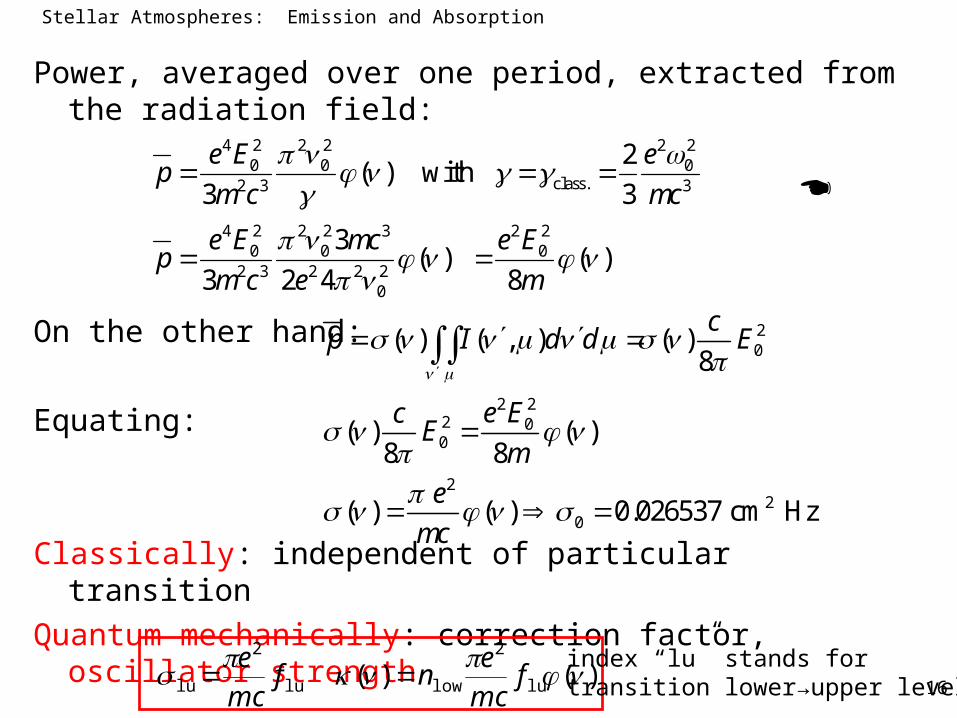
Power, averaged over one period, extracted from the radiation field:
On the other hand:
Equating:
Classically: independent of particular transition
Quantum mechanically: correction factor, oscillator strength
4 2 2 2 2 20 0 0
class.2 3 3
4 2 2 2 3 2 20 0 0
2 3 2 2 20
2( ) with
3 3
3( ) ( )
3 2 4 8
e E ep
m c mc
e E mc e Ep
m c e m
20
2 22 00
22
0
( ) ( , ) ( )8
( ) ( )8 8
( ) ( ) 0.026537 cm Hz
cp I d d E
e EcE
m
e
mc
)()( lu
2
lowlu
2
lu fmc
enf
mc
e
index “lu” stands for transition lower→upper level
Stellar Atmospheres: Emission and Absorption
17
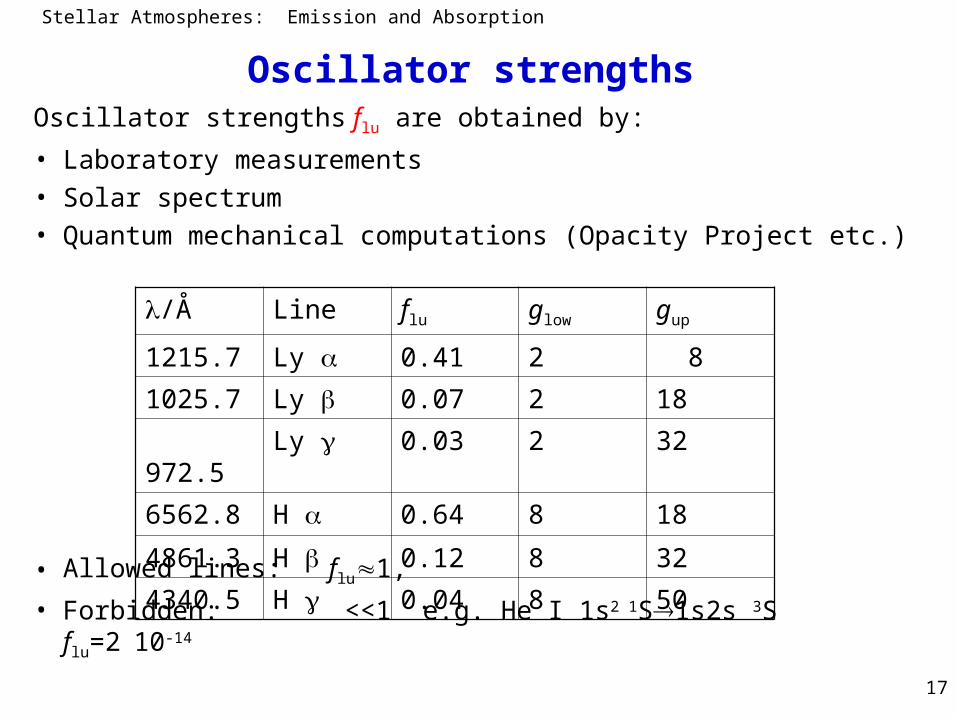
Oscillator strengthsOscillator strengths flu are obtained by:
• Laboratory measurements• Solar spectrum• Quantum mechanical computations (Opacity Project etc.)
• Allowed lines: flu1,
• Forbidden: <<1 e.g. He I 1s2 1S1s2s 3S flu=210-14
/Å Line flu glow gup
1215.7 Ly 0.41 2 8
1025.7 Ly 0.07 2 18
972.5 Ly 0.03 2 32
6562.8 H 0.64 8 18
4861.3 H 0.12 8 32
4340.5 H 0.04 8 50
Stellar Atmospheres: Emission and Absorption
18
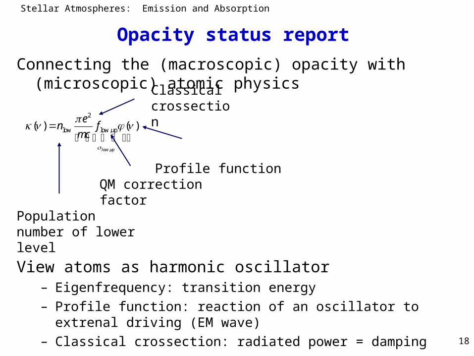
Opacity status report
Connecting the (macroscopic) opacity with (microscopic) atomic physics
View atoms as harmonic oscillator– Eigenfrequency: transition energy– Profile function: reaction of an oscillator to extrenal driving (EM wave)– Classical crossection: radiated power = damping
,
2
low low,up( ) ( )
low up
en f
mc
Population number of lower level
QM correction factorProfile function
Classical crossection
Stellar Atmospheres: Emission and Absorption
19
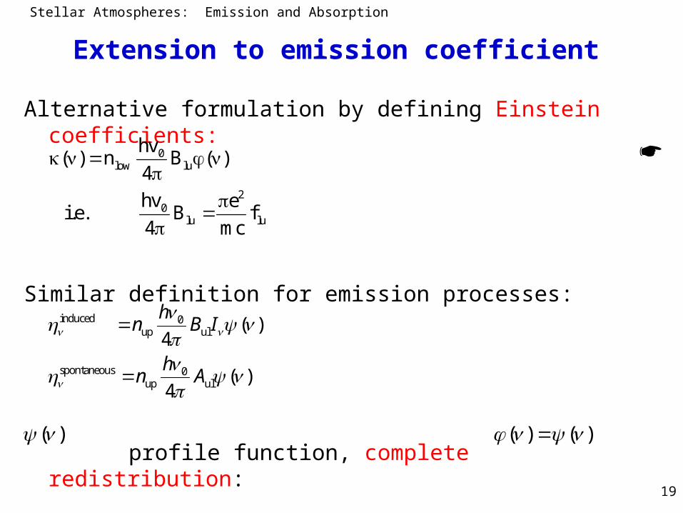
Extension to emission coefficient
Alternative formulation by defining Einstein coefficients:
Similar definition for emission processes:
profile function, complete redistribution:
induced 0up ul
spontaneous 0up ul
( )4
( )4
hn B I
hn A
0low lu
20
lu lu
hv( ) n B ( )
4
hv e i.e. B f
4 mc
)( )()(
Stellar Atmospheres: Emission and Absorption
20
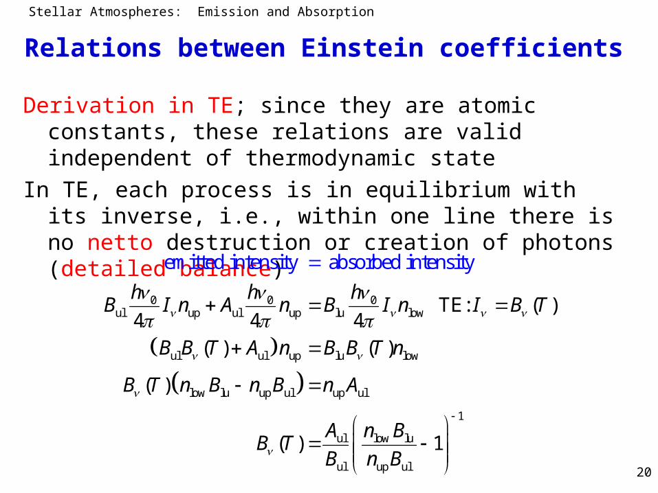
Relations between Einstein coefficients
Derivation in TE; since they are atomic constants, these relations are valid independent of thermodynamic state
In TE, each process is in equilibrium with its inverse, i.e., within one line there is no netto destruction or creation of photons (detailed balance)
0 0 0ul up ul up lu low
ul ul up lu low
low lu up ul up ul
1
ul low lu
ul up ul
TE: ( )4 4 4
( ) ( )
(
emitted intensity absorbed inte
)
nsity
( ) 1
h h hB I n A n B I n I B T
B B T A n B B T n
B T n B n B n A
A n BB T
B n B
Stellar Atmospheres: Emission and Absorption
21
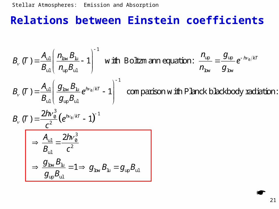
Relations between Einstein coefficients
0
0
0
1
up upul low lu
ul up ul low low
1
ul low lu
ul up ul
31
02
( ) 1 with Boltzmann equation:
( ) 1 comparison with Planck blackbody radiation:
2( ) 1
h kT
h kT
h kT
n gA n BB T e
B n B n g
A g BB T e
B g B
hB T e
c
3
ul 02
ul
low lulow lu up ul
up ul
2
1
A h
B c
g Bg B g B
g B

Stellar Atmospheres: Emission and Absorption
22
Relation to oscillator strength
dimension
Interpretation of as lifetime of the excited state
order of magnitude:
at 5000 Å:
lifetime:
2 2
lu lu0
2 2up up
ul lu lulow low 0
3 2 2 2up up0 0
ul ul lu ul lu2 3low low
4
4
2 83
eB f
mchv
g g eB B f
g g mchv
g ghv e vA B f f
c g mc g
ulA 1 time
ul1 A
ulul A18 s10
s10 8
Stellar Atmospheres: Emission and Absorption
23
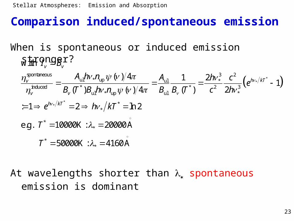
Comparison induced/spontaneous emission
When is spontaneous or induced emission stronger?
At wavelengths shorter than spontaneous emission is dominant
**
**
spontaneous 3 2ul * up ul *
induced * * 2 3ul * up ul *
**
*
*
with
( ) 4 211
( ) ( ) 4 ( ) 2
: 1 2 ln 2
e.g. 10000K : 20000A
50000K : 4160A
v v
h kTv
v v
h kT
*
*
I B
A h n A h ce
B T B h n B B T c h
e h kT
T
T

Stellar Atmospheres: Emission and Absorption
24
Induced emission as negative absorptionRadiation transfer equation:
Useful definition: corrected for induced emission:
spontaneous induced
spontaneous induced
induced0 0lu lu low lu ul up
with
( ), ( )4 4
v
dII
dsdI
Ids
h hB n B n I
spontaneous 0ul up lu low
2low
lu lu low upup
3 2spontaneous 0 lowlu lu up2
up
( ) 4
( )
2 ( )
dI hB n B n I
ds
gef n n
mc g
h gef n
c mc g
transition low→up
So we get (formulated withoscillator strength insteadof Einstein coefficients):
Stellar Atmospheres: Emission and Absorption
25
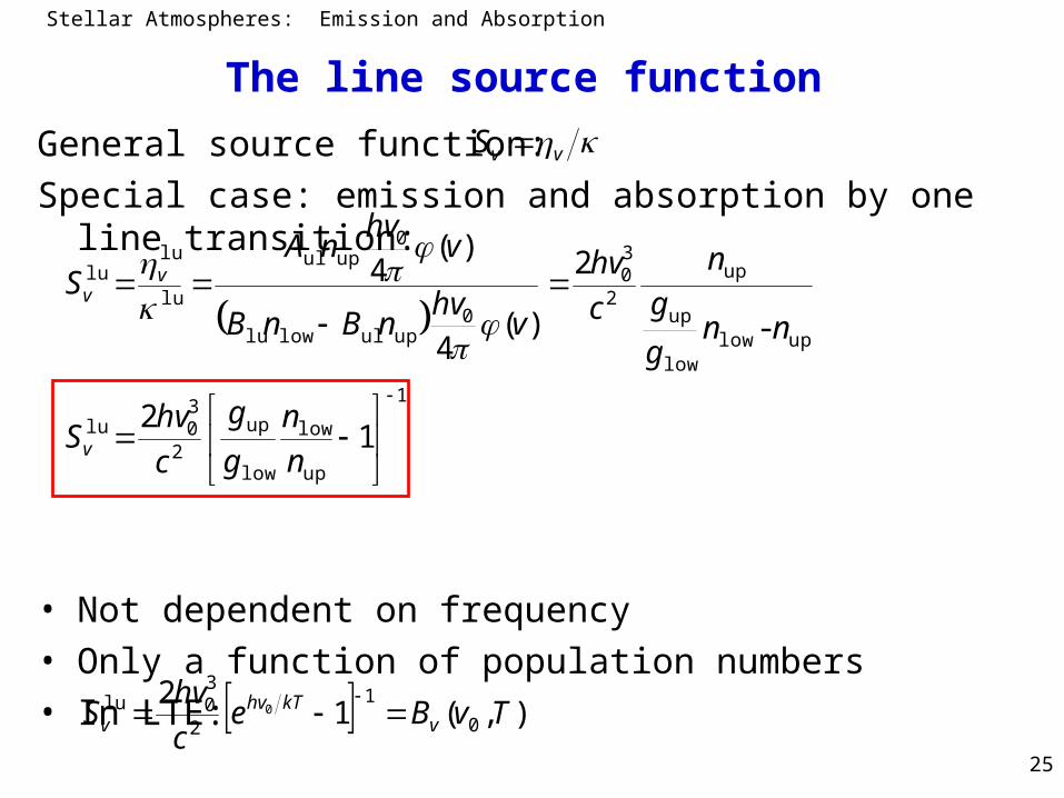
The line source function
General source function:
Special case: emission and absorption by one line transition:
• Not dependent on frequency• Only a function of population numbers• In LTE:
vvS
1
up
low
low
up
2
30lu
uplowlow
up
up
2
30
0upullowlu
0upul
lu
lulu
12
-
2
)(4
)(4
n
n
g
g
c
hvS
nng
g
n
c
hv
vhv
nBnB
vhv
nAS
v
vv
),(12
0
1
2
30lu 0 TvBe
c
hvS v
kThvv

Stellar Atmospheres: Emission and Absorption
26
Every energy level has a finite lifetime against radiative decay (except ground level)
Heisenberg uncertainty principle:
Energy level not infinitely sharp
q.m. profile function = Lorentz profile
Simple case: resonance lines (transitions to ground state)example Ly (transition 21):
example H (32):
Line broadening: Radiation damping
ul
ul1 A
E
l
ll
AAj
juk
uku
11
21 cl 1 2 12A 3 g g f cl cl3 2 8 0.41 0.31
1 2 1cl 12 23 13 cl cl
2 3 3
g g g 2 8 23 f f f 3 0.41 0.64 0.07 1.18
g g g 8 18 18
Stellar Atmospheres: Emission and Absorption
27
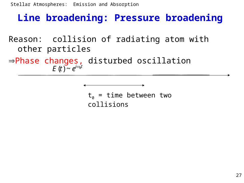
Line broadening: Pressure broadening
Reason: collision of radiating atom with other particles
Phase changes, disturbed oscillation
t0 = time between two collisions
0( ) ~ i tE t e
Stellar Atmospheres: Emission and Absorption
30
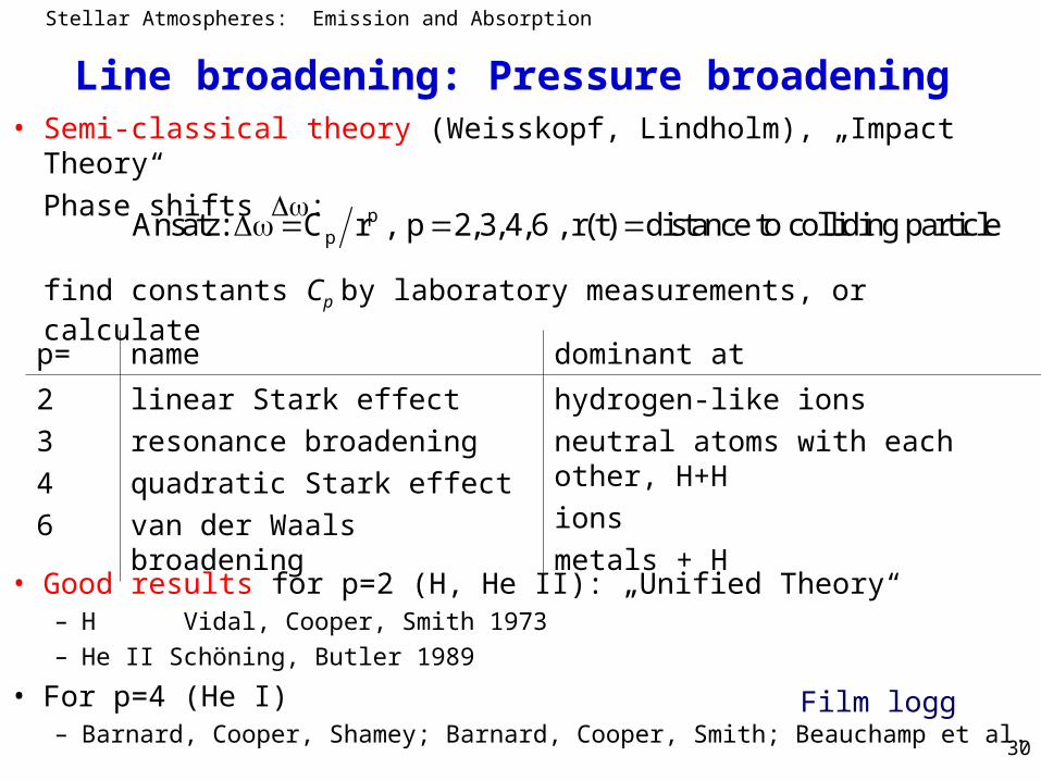
Line broadening: Pressure broadening• Semi-classical theory (Weisskopf, Lindholm), „Impact Theory“
Phase shifts :
find constants Cp by laboratory measurements, or calculate
• Good results for p=2 (H, He II): „Unified Theory“– H Vidal, Cooper, Smith 1973– He II Schöning, Butler 1989
• For p=4 (He I)– Barnard, Cooper, Shamey; Barnard, Cooper, Smith; Beauchamp et al.
ppAnsatz: C r , p 2,3,4,6 , r(t) distance to colliding particle
p= name dominant at
2
3
4
6
linear Stark effect
resonance broadening
quadratic Stark effect
van der Waals broadening
hydrogen-like ions
neutral atoms with each other, H+H
ions
metals + H
Film logg
Stellar Atmospheres: Emission and Absorption
31
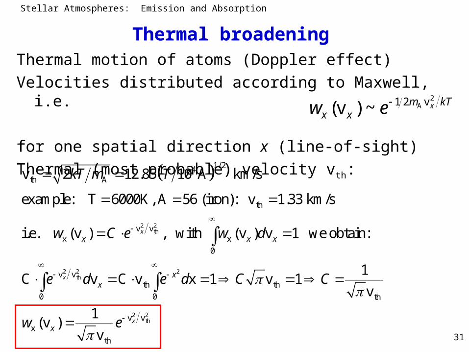
Thermal broadeningThermal motion of atoms (Doppler effect)
Velocities distributed according to Maxwell, i.e.
for one spatial direction x (line-of-sight)
Thermal (most probable) velocity vth:
kTmxx
xew2
A v21~)v(
2 2th
2 2 2th
1/ 24th A
th
v vx x
0
v vth th
0 0 th
x
v 2 12.85 10 A km/s
example: T 6000K, A 56 (iron): v 1.33 km/s
i.e. (v ) , with (v ) v 1 we obtain:
1C v C v x 1 v 1
v
(v )
x
x
x x x
xx
x
kT m T
w C e w d
e d e d C C
w
2 2
thv v
th
1
vxe
Stellar Atmospheres: Emission and Absorption
32
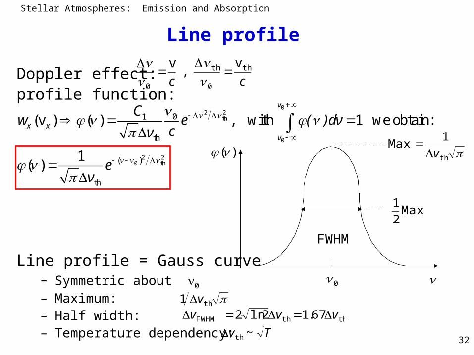
Line profile
Doppler effect:profile function:
Line profile = Gauss curve– Symmetric about 0
– Maximum:– Half width:– Temperature dependency:
ccth
0
th
0
v ,
v
02 2
th
0
2 20 th
01
th
( )
th
(v ) ( ) , with 1 we obtain:
1( )
ν
x x
ν
Cw e ( )dν
cν
eν
th
1Max
v
Max2
1
0
)(
FWHM
th1 v
ththFWHM 67.12ln2 vvv Tv ~th
Stellar Atmospheres: Emission and Absorption
33
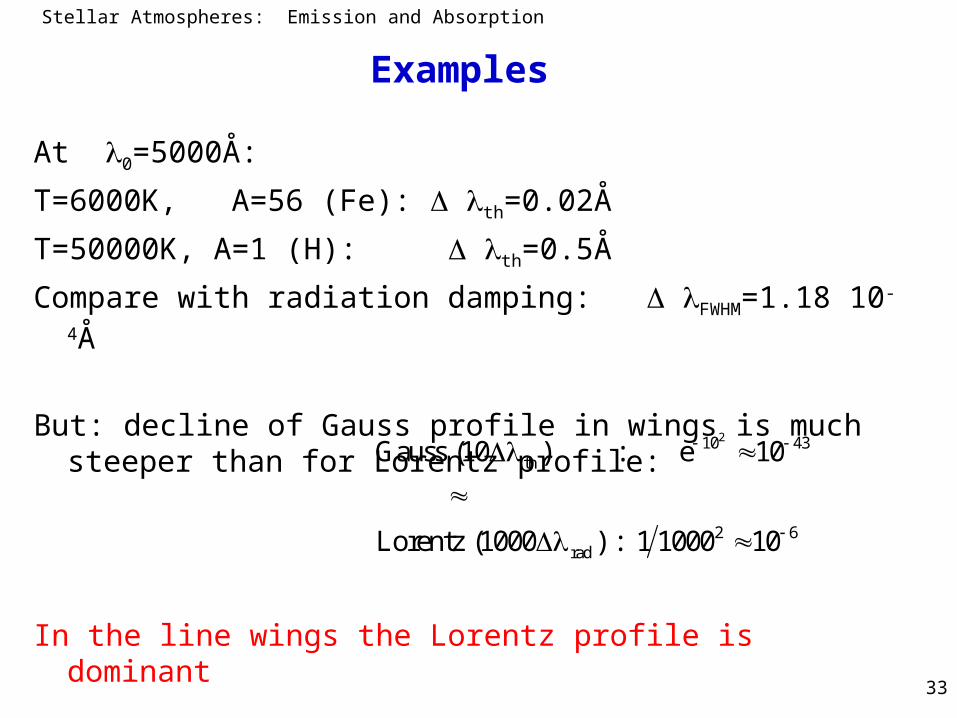
Examples
At 0=5000Å:
T=6000K, A=56 (Fe): th=0.02Å
T=50000K, A=1 (H): th=0.5Å
Compare with radiation damping: FWHM=1.18 10-4Å
But: decline of Gauss profile in wings is much steeper than for Lorentz profile:
In the line wings the Lorentz profile is dominant
210 43th
2 6rad
Gauss (10 ) : e 10
Lorentz (1000 ) : 1 1000 10
Stellar Atmospheres: Emission and Absorption
34
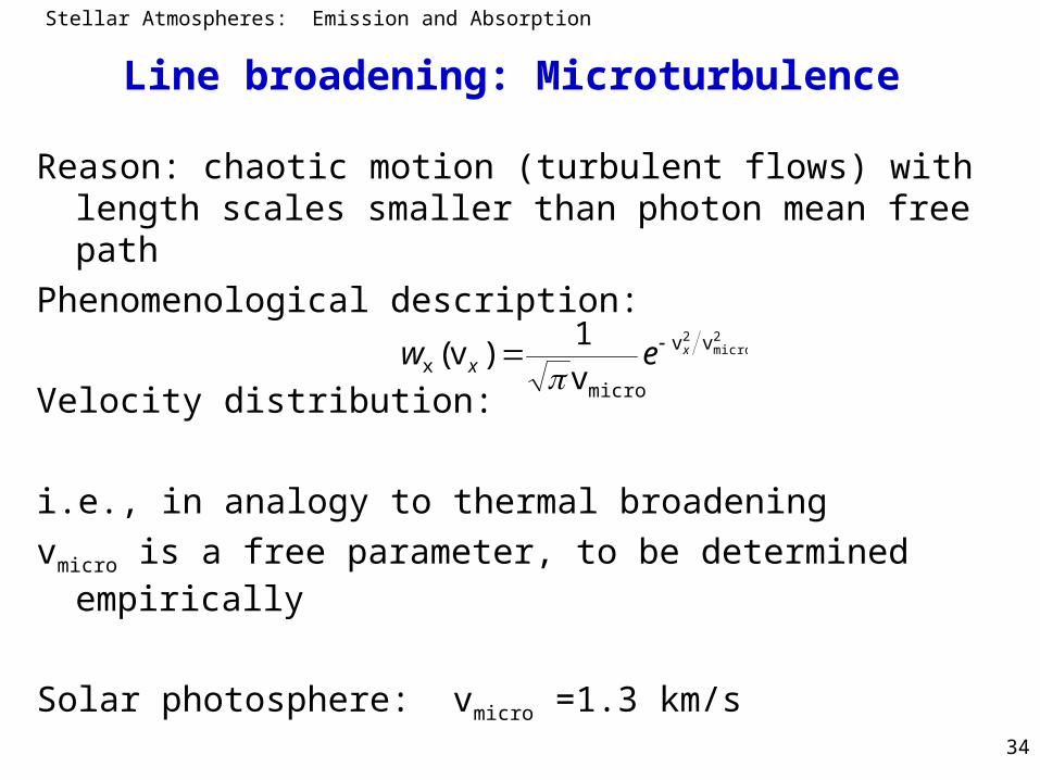
Line broadening: Microturbulence
Reason: chaotic motion (turbulent flows) with length scales smaller than photon mean free path
Phenomenological description:
Velocity distribution:
i.e., in analogy to thermal broadening
vmicro is a free parameter, to be determined empirically
Solar photosphere: vmicro =1.3 km/s
2micro
2 vv
microx v
1)v( xew x

Stellar Atmospheres: Emission and Absorption
35
Joint effect of different broadening mechanisms
Mathematically: convolution
commutative:
multiplication of areas:
Fourier transformation:
y y xx
x profile A + profile B = joint effect
dxxfdxxfdxxff BABA
)()())((
ABBA ffff
dyyxfyfxff BABA )()())((
BABA ffff ~~
2~
i.e.: in Fourier space the convolution is a multiplication
Stellar Atmospheres: Emission and Absorption
36
Application to profile functions
Convolution of two Gauss profiles (thermal broadening + microturbulence)
Result: Gauss profile with quadratic summation of half-widths; proof by Fourier transformation, multiplication, and back-transformationConvolution of two Lorentz profiles (radiation + collisional damping)
Result: Lorentz profile with sum of half-widths; proof as above
2 2 2 2
2 2 2 2 2C
( ) 1 ( ) 1
G ( ) ( ) ( ) 1 with C
x A x BA B
x CA B
G x A e G x B e
x G x G x C e A B
2 2 2 2
2 2
/ /( ) ( )
/( ) ( ) ( ) with
A B
C A B
A BL x L x
x A x BC
L x L x L x C A Bx C
Stellar Atmospheres: Emission and Absorption
37
Application to profile functions
Convolving Gauss and Lorentz profile (thermal broadening + damping)
2 2
0
2
2( )
220
0 0
2
1 / 4( )
( ) / 4
depends on , , : ( )́ ´ ´
Transformation: v: : 4 : ´
/1( )
D
D
D
D D D
y D
D
G e L( )
V G L Δ V( ) G L(v )d
( ) Δ a /( πΔ ) y ( ) Δ
aG y e L(y)
y
2
2
2 2 2
2 2
Voigt fu
1
(v )
1Def: ( , v) with ( , v)
(v )
, no analytical representation possible.
(approximate formulae or numerical evaluation)
Norm
nc
a
o
l
ti n
y
D
y
D
a eV dy
a y a
a eV H a H a dy
y a
ization: ( , v) v
H a d

Stellar Atmospheres: Emission and Absorption
38
Voigt profile, line wings
Stellar Atmospheres: Emission and Absorption
39
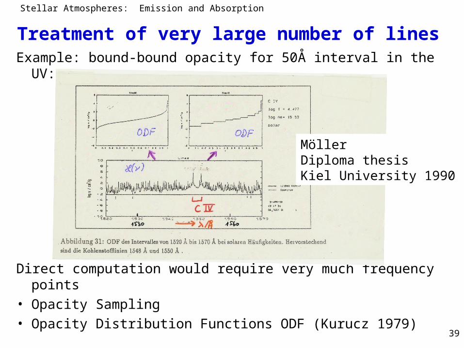
Treatment of very large number of linesExample: bound-bound opacity for 50Å interval in the UV:
Direct computation would require very much frequency points• Opacity Sampling• Opacity Distribution Functions ODF (Kurucz 1979)
MöllerDiploma thesisKiel University 1990
Stellar Atmospheres: Emission and Absorption
40
Bound-free absorption and emission
Einstein-Milne relations, Milne 1924: Generalization of Einstein relations to continuum processes: photoionization and recombination
Recombination spontaneous + induced
Transition probabilities:
I) number of photoionizations
II) number of recombinations
Photon energy
In TE, detailed balancing: I) = II)
: probability for photoionization in
(v) : spontaneous recapture probability of electron in v, v v
(v) : corresponding induced probability v=electron velocity
P d
F d
G
dtdIGFnn v vv)v()v()v(eup
dtdIPn vv low
v vv21 2ion dhmdvmEhv

Stellar Atmospheres: Emission and Absorption
41
Einstein-Milne relations
low up e
low up e
13
1low
2up e
3
2
low
up e
low up
(v) (v) (v) with
(v) (v) (v)
(v) 21 1
(v) (v) (v)
(v) 2
(v)
(v) (v)
f
v
v
h kTv
h kTv
n P I dvdt n n F G I h m dvdt I B
n P B n n F G B h m
n P mF hB e
G n n hG c
F h
G c
n P me
n n hG
n n
ion
2
3/ 2uplow
2up e low
3/ 2v 2 2
e e e
2 2rom Saha equation:
(v) : Maxwell distribution: (v) v 4 v v2
E kT
m kT
gn mkTe
n n h g
mn n d n e d
kT
Stellar Atmospheres: Emission and Absorption
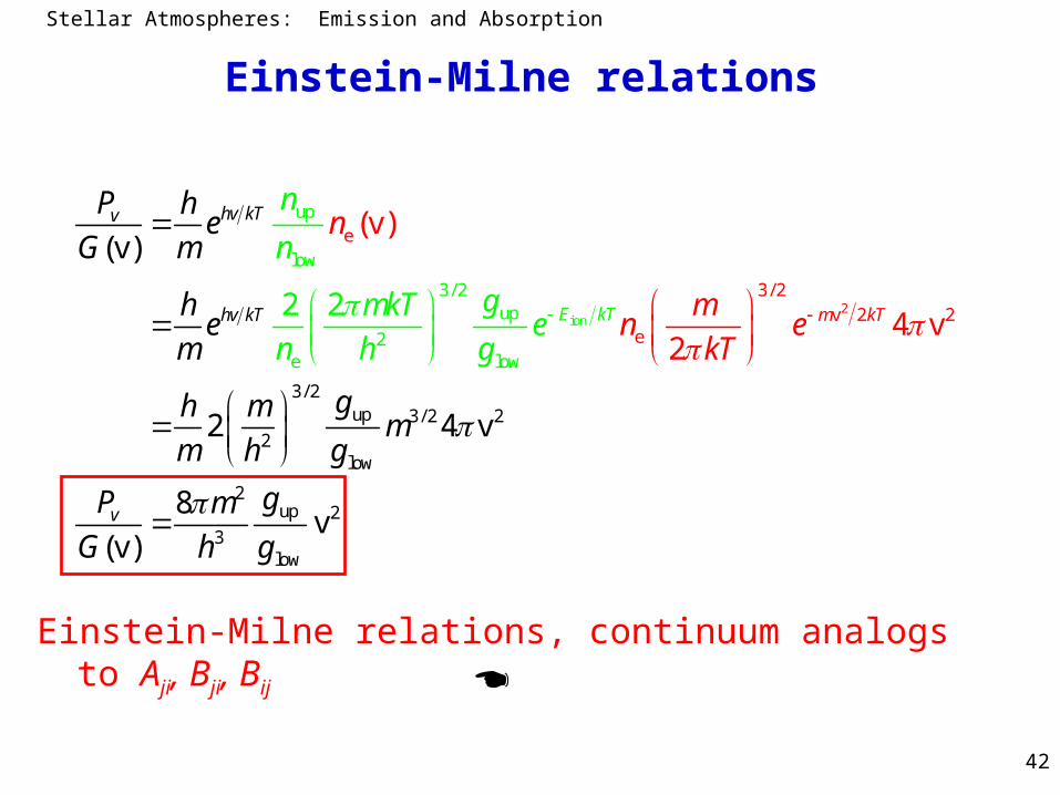
42
Einstein-Milne relations
Einstein-Milne relations, continuum analogs to Aji, Bji, Bij
2ion
3/ 2up 3/ 2
up
low
3
22
low
2up 2
3lo
/ 2up
2e low
e
3/ 2v 2 2
e
w
(v)
2 4 v
8
(v)
4 v2
v(v
2 2
)
hv kT
m kTE kT
v
hv kT
v
n
mn e
kT
P he
G m
he
m
gh mm
n
n
gmkT
m h g
gP m
G h g
en h g
Stellar Atmospheres: Emission and Absorption
43
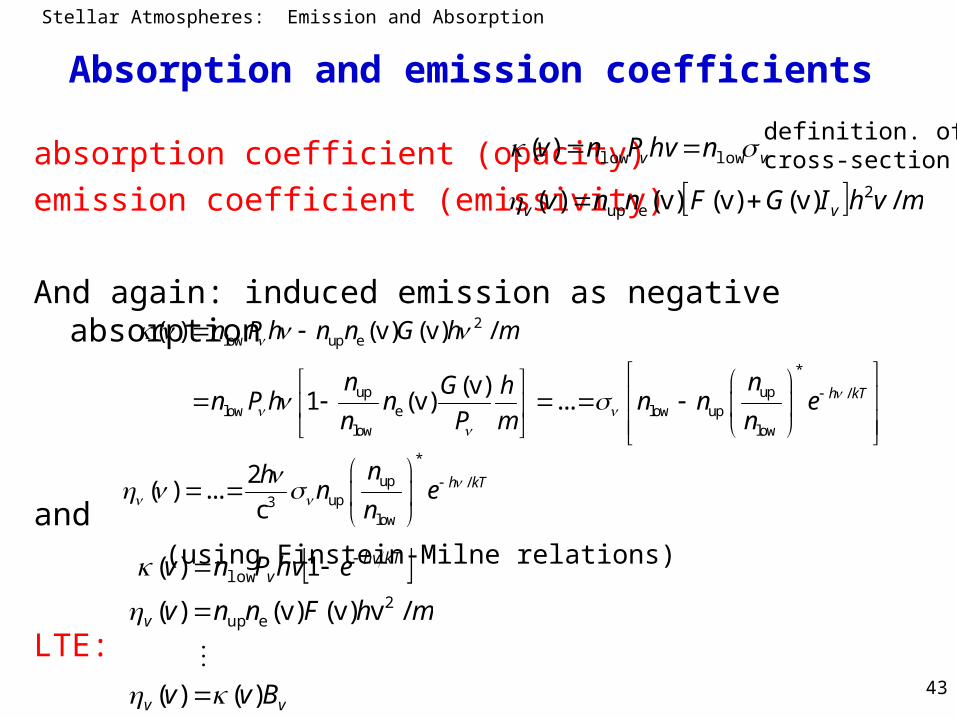
Absorption and emission coefficients
absorption coefficient (opacity)
emission coefficient (emissivity)
And again: induced emission as negative absorption
and (using Einstein-Milne relations)
LTE:
vv nhvPnv lowlow)(
mvhIGFnnv vv /)v()v()v()( 2eup
2low up e
*
up up /low e low up
low low
( ) (v) (v) /
(v)1 (v) ... h kT
n P h n n G h m
n nG hn P h n n n e
n P m n
vv
v
kThvv
Bvv
mhFnnv
ehvPnv
)()(
/v)v()v()(
1)(2
eup
low
*
up /up3
low
2( ) ...
ch kTnh
n en
definition. of cross-section

Stellar Atmospheres: Emission and Absorption
44
Continuum absorption cross-sections
H-like ions: semi-classical Kramers formula
Quantum mechanical calculations yield correction factors
Adding up of bound-free absorptions from all atomic levels: example hydrogen
3
th th th
318 2
th th 2 22 2 2
for ( )
0 else
8 threshold frequency, 7.906 10 cm
3 3 principal quantum number, Z nuclear charge
h n n
Z Zm cen
3
th th bf bf( ) ( , ) , ( , ) Gaunt factorg n g n
max
1bf
totbf )()(
n
nn
n nvv

Stellar Atmospheres: Emission and Absorption
45
Continuum absorption cross-sections
Optical continuum dominated by Paschen continuum
Stellar Atmospheres: Emission and Absorption
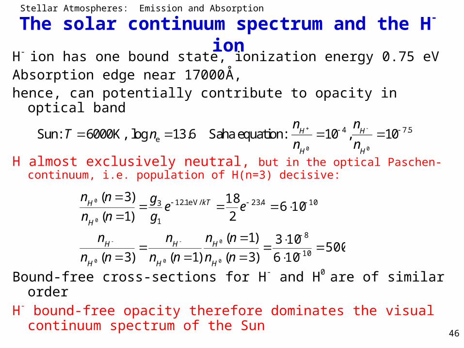
46
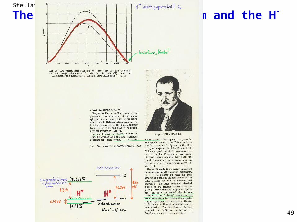
The solar continuum spectrum and the H- ionH- ion has one bound state, ionization energy 0.75 eVAbsorption edge near 17000Å,hence, can potentially contribute to opacity in optical band
H almost exclusively neutral, but in the optical Paschen-continuum, i.e. population of H(n=3) decisive:
Bound-free cross-sections for H- and H0 are of similar order
H- bound-free opacity therefore dominates the visual continuum spectrum of the Sun
0 0
4 7.5eSun: 6000K, log 13.6 Saha equation: 10 , 10H H
H H
n nT n
n n
500106
103
)3(
)1(
)1()3(
1062
18
)1(
)3(
10
8
104.23/eV1.12
1
3
0
0
00
0
0
nn
nn
nn
n
nn
n
eeg
g
nn
nn
H
H
H
H
H
H
kT
H
H
Stellar Atmospheres: Emission and Absorption
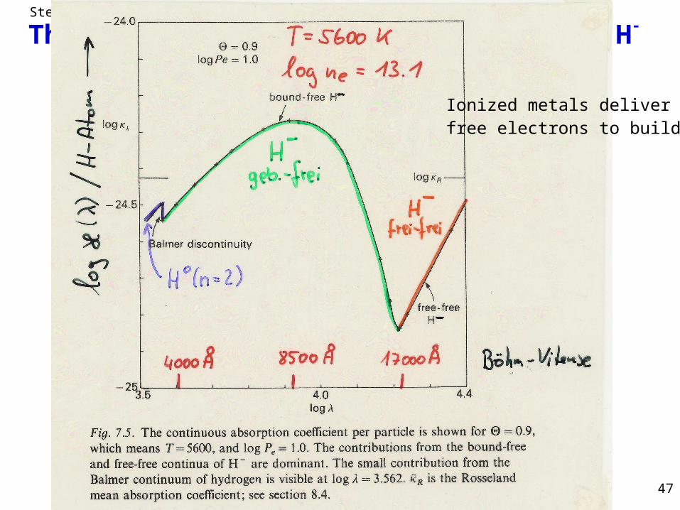
47
The solar continuum spectrum and the H- ion
Ionized metals deliver free electrons to build H
-
Stellar Atmospheres: Emission and Absorption
49
The solar continuum spectrum and the H- ion

Stellar Atmospheres: Emission and Absorption
54
Free-free absorption and emission
Assumption (also valid in non-LTE case):
Electron velocity distribution in TE, i.e. Maxwell distribution
Free-free processes always in TE
Similar to bound-free process we get:
generalized Kramers formula, with Gauntfaktor from q.m.• Free-free opacity important at higher energies, because
less and less bound-free processes present• Free-free opacity important at high temperatures
),()(/)()( ffffff TvBvvvS vvv
ff h / kTff e k
2 2 6
ff ff3/ 2 3
( ) ( )n n 1 e
16 Z e( ) g (n, ,T)
hc(2 T
1
m)3 3
1
1/ 2 3/ 2ffff bf bf~ T , but ~ T (Saha), therefore: / T
Stellar Atmospheres: Emission and Absorption
55
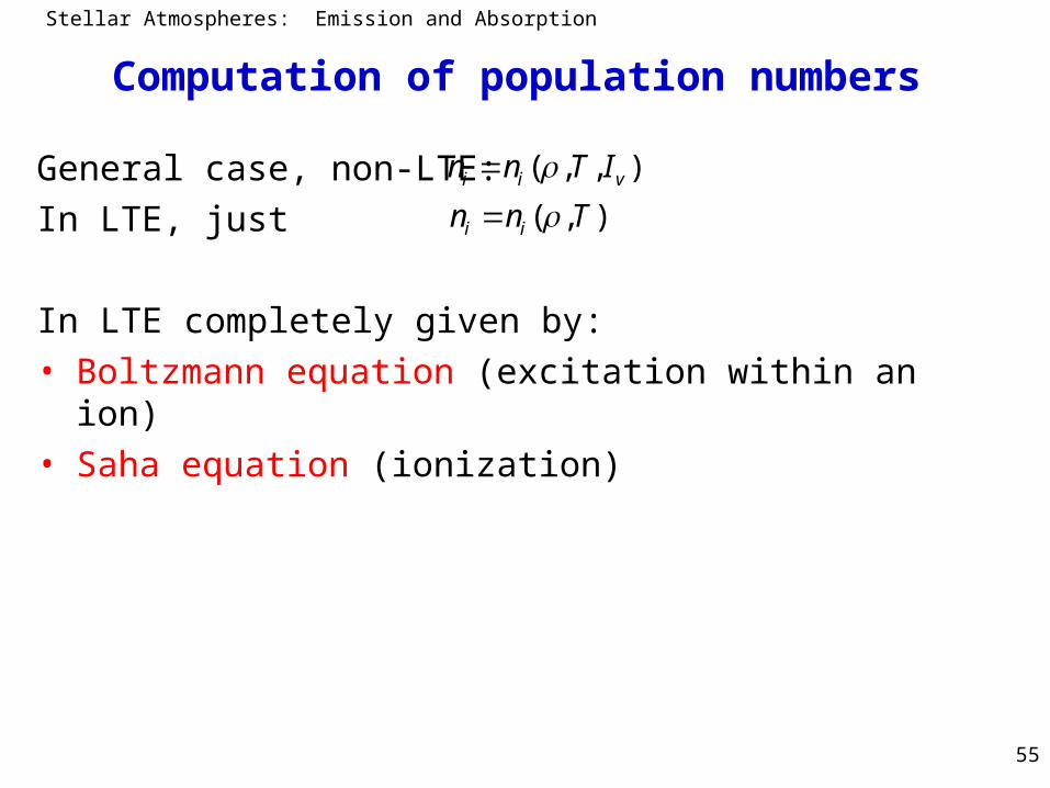
Computation of population numbers
General case, non-LTE:
In LTE, just
In LTE completely given by:• Boltzmann equation (excitation within an ion)• Saha equation (ionization)
( , , )i i vn n T I
( , )i in n T

Stellar Atmospheres: Emission and Absorption
56
Boltzmann equationDerivation in textbooks
Other formulations:
• Related to ground state (E1=0)
• Related to total number density N of respective ion
( ) / statistical weight
excitation energy i jE E kT ii i
ij j
gn ge
En g
kTEii ieg
g
n
n /
11
1 1
1 1 1
1
1
1
/
/partition function(
1
, with ( ) :)
j
jE kTj
i i i i
jj j
i i
E kTj
n n n nn gnn n n n nn
g e
U T
n n gU g
nT
Ne

Stellar Atmospheres: Emission and Absorption
57
Divergence of partition function
e.g. hydrogen:
Normalization can be reached only if number of levels is finite.
Very highly excited levels cannot exist because of interaction with neighbouring particles, radius H atom:
At density 1015 atoms/cm3 mean distance about 10-5 cm
r(nmax) = 10-5 cm nmax ~43
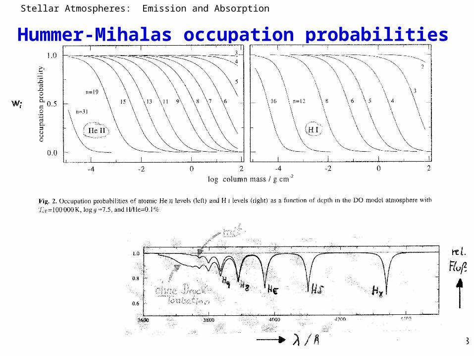
Levels are “dissolved“; description by concept of occupation probabilities pi (Mihalas, Hummer, Däppen 1991)
i
2i i i Ion
E / kTi
g 2n g , E E
i.e. g e
i i
i
lim lim
lim
Nni
i
20)( nanr
with w0 hen i i iig pg p i
Stellar Atmospheres: Emission and Absorption
58
Hummer-Mihalas occupation probabilities
Stellar Atmospheres: Emission and Absorption
59
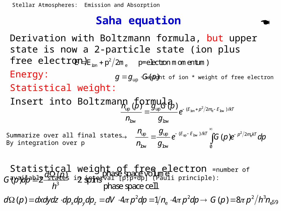
Saha equation
Derivation with Boltzmann formula, but upper state is now a 2-particle state (ion plus free electron)
Energy:
Statistical weight:
Insert into Boltzmann formula
Statistical weight of free electron =number of available states in interval [p,p+dp] (Pauli principle):
2ion eE E p 2m p=electron momentum)
)(up pGgg
2ion e low
2up low e
up up ( 2 ) /
low low
( ) /up up 2
low low 0
( ) ( )
( )
E p m E kT
E E kT p m kT
n p g G pe
n g
n ge G p e dp
n g
3
2 2 2 3e e
phase space volume( )( ) 2 2 spins
phase space cell
( ) 4 1 4 ( ) 8x y z
d pG p dp
h
d p dxdydz dp dp dp dV p dp n p dp G p p h n
weight of ion * weight of free electron
Summarize over all final statesBy integration over p

Stellar Atmospheres: Emission and Absorption
60
Saha equation
Insertion into Boltzmann formula gives:
Saha equation for two levels in adjacent ionization stages
Alternative:
2up low e
2up low
up low
up
( ) /up up 22e3
low low e0
3/ 2( ) /up 2e3
low e 0
3/ 2( ) /upe3
low e
3/ 2(up upe
3low e low
8 with / 2
82
82
4
22
E E kT p mkT
E E kT x
E E kT
E
n ge p e dp x p m kT
n g h n
ge m kT x e dx
g h n
ge m kT
g h n
n gm kTe
n n h g
low ) /E kT
33/216/)(
low
up2/3
low
eup cm K 1007.2 )( lowup Ceg
g
C
TTf
n
nn kTEE
Stellar Atmospheres: Emission and Absorption
61
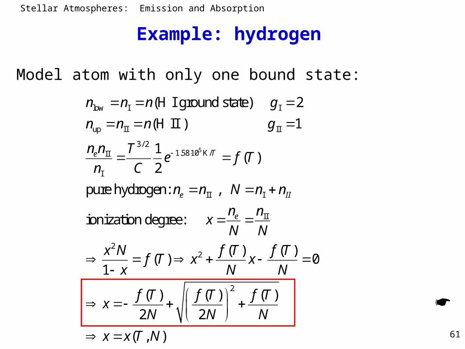
Example: hydrogen
Model atom with only one bound state:
5
low I I
up II II
3/ 21.58 10 K/II
I
II I
II
22
(H I ground state) 2
(H II ) 1
1( )
2
pure hydrogen: ,
ionization degree:
(( )
1
Te
e II
e
n n n g
n n n g
n n Te f T
n C
n n N n n
n n x
N N
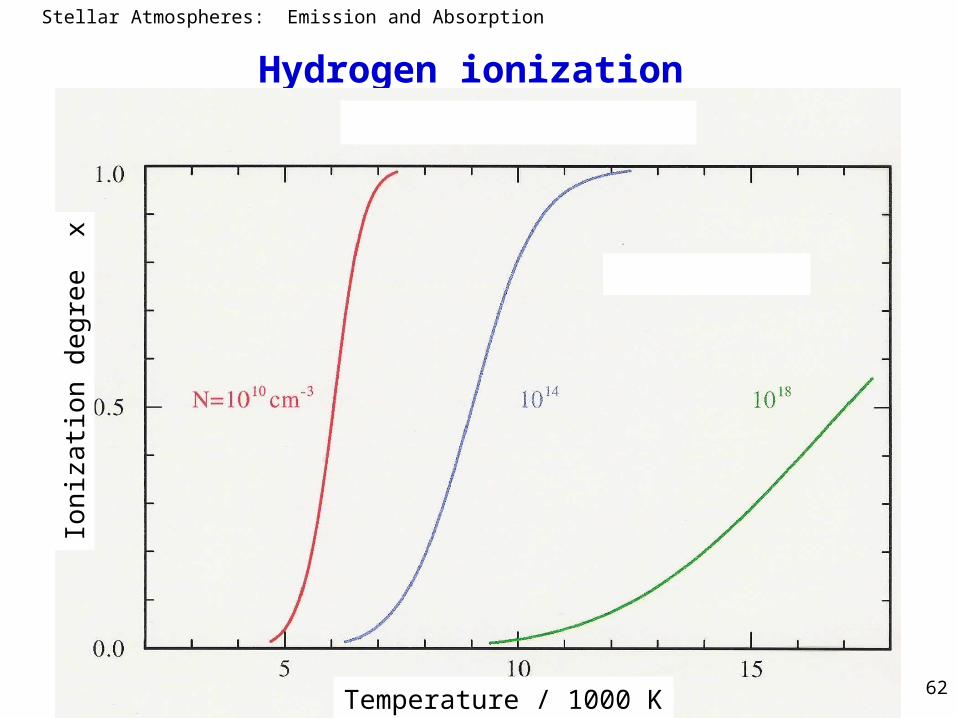
x N f Tf T x
x
2
) ( )0
( ) ( ) ( )
2 2
( , )
f Tx
N N
f T f T f Tx
N N N
x x T N
Stellar Atmospheres: Emission and Absorption
62
Hydrogen ionization
Ion
iza
tion
de
gre
e x
Temperature / 1000 K
Stellar Atmospheres: Emission and Absorption
63
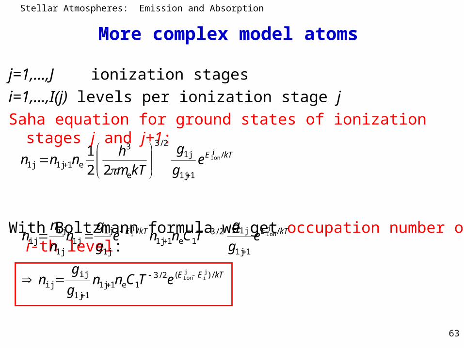
More complex model atoms
j=1,...,J ionization stages
i=1,...,I(j) levels per ionization stage j
Saha equation for ground states of ionization stages j and j+1:
With Boltzmann formula we get occupation number of i-th level:
kTEeg
g
kTm
hnnn /
11j
1j2/3
e
3
e1j1j1
jIon
22
1
kTEE
kTEkTE
eTCnng
gn
eg
gTCnne
g
gn
n
nn
/)(2/31e1j1
11j
ijij
/
11j
1j2/31e1j1
/
1j
ij1j
1j
ijij
ji
jIon
jIon
ji
Stellar Atmospheres: Emission and Absorption
64
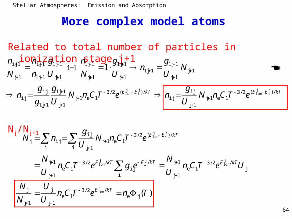
More complex model atoms
Related to total number of particles in ionization stage j+1
Nj/Nj+1
kTEEkTEE eTCnNU
gneTCnN
U
g
g
gn
NU
gn
U
g
N
n
U
g
n
n
N
n
/)(2/31e1j
1j
ijij
/)(2/31e1j
1j
11j
11j
ijij
1j1j
11j11j
1j
11j
1j
11j
1j
11j
11j
1ij
1j
1ij
ji
jIon
ji
jIon
1 1i
)(je/2/3
1e1j
j
1j
j
j/2/3
1e1j
1j
i
/ij
/2/31e
1j
1j
i
/)(2/31e1j
1j
ij
iijj
jIon
jIon
ji
jIon
ji
jIon
TneTCnU
U
N
N
UeTCnU
NegeTCn
U
N
eTCnNU
gnN
kTE
kTEkTEkTE
kTEE
Stellar Atmospheres: Emission and Absorption
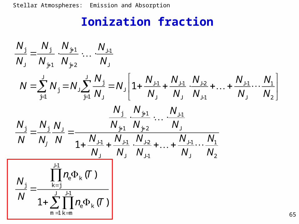
65
Ionization fraction
j j j 1 J-1
J j 1 j 2 J
J Jj J-1 J-1 J-2 J-1 1
j J Jj 1 j 1 J J J J-1 J 2
j j 1 J-1
j j j 1 j 2 JJ
J-1 J-1 J-2 J-1 1
J J J-1 J 2
J-1
e kj k j
e kk
1
1
( )
1 ( )
J
N N N N
N N N N
N N N N N NN N N N
N N N N N N
N N N
N N N N NNN N N N NN N NN N N N N
n TN
Nn T
J-1J
m 1 m

Stellar Atmospheres: Emission and Absorption
66
Ionization fractions

Stellar Atmospheres: Emission and Absorption
67
Summary: Emission and Absorption
Stellar Atmospheres: Emission and Absorption
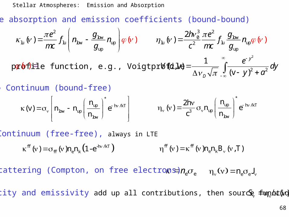
68
● Line absorption and emission coefficients (bound-bound)32 2
low 0 lowlu lu low up lu lu up2
up up
( ) 2
( ) ( ) ( )
g h ge ef n n f n
mc g c mc g
profile function, e.g., Voigtprofile( ) 2
2 2
1( , v)
(v )
y
D
eV a dy
y a
● Continuum (bound-free)*
up h / kTlow up
low
n(v) n n e
n
*
up h / kTup3
low
n2h( ) n e
c n
● Continuum (free-free), always in LTE
ff -h / kTff e k( ) ( )n n 1- e ff ff
e k( ) ( )n n B ( ,T)
ee n● Scattering (Compton, on free electrons)e en J
Total opacity and emissivity add up all contributions, then source function S ( )
Stellar Atmospheres: Emission and Absorption
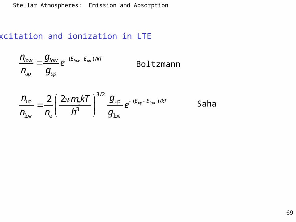
69
Excitation and ionization in LTE
( ) / low upE E kTlow low
up up
n ge
n g
up low
3/ 2( ) /up upe
3low e low
22
E E kTn gm kTe
n n h g
Boltzmann
Saha


