Steroids, Home Runs and the Law of Genius Arthur De Vany Professor Emeritus Department of Economics Institute for Mathematical Behavioral Sciences University of California, Irvine www.arthurdevany.com [email protected]ABSTRACT The greatest home run hitters are as rare as great scientists, artists, or composers. The greatest accomplishments in these fields all follow the same universal law of genius, as I show in this paper. There is no evidence that steroid use has altered home run hitting and those who argue otherwise are profoundly ignorant of the statistics of home runs, the physics of baseball, and of the physiological effects of steroids. There is no standard for great accomplishments, in home runs, in the sciences, and in the arts. Genius has its own way and the great achievements of McGwire, Sosa, and Bonds (they did it in that order) are of a piece with genius in other fields — they are the Bach, Beethoven, and Mozart of home runs. The law of home runs established here generalizes the laws of extreme accomplish- ment developed by Pareto, Lotka, Price and Charles Murray. Economics seems to have little place for genius, but the growing importance of intellectual property calls for a greater understanding of extreme accomplishment. The stable Paretian model devel- oped here will be of use to economists studying extreme accomplishment in other areas and has led to a new understanding of the motion picture industry (De Vany, 2004). 1. Introduction Six bills are before Congress to impose drug testing and penalties on major league baseball and other professional sports (Kiele 2005). A Senate hearing was held this year in which Jose Canseco, Mark McGwire, and Rafael Palmeiro testified about steroid use in MLB. Many appear to believe that steroid use has caused an increase in home runs. Arguing that Palmeiro’s suspension for testing positive for steroids has pushed the issue into the policy arena, Senators Stevens, McCain, and Hall of Fame pitcher and now Senator Jim Bunning are cosponsoring drug-testing bills. The intent of Congress can be inferred from the title of the hearings: “Restoring Faith in America’s Pastime”.
Transcript
Steroids, Home Runs and the Law of Genius
Arthur De Vany
Professor EmeritusDepartment of Economics
Institute for Mathematical Behavioral SciencesUniversity of California, Irvine
The greatest home run hitters are as rare as great scientists, artists, or composers.The greatest accomplishments in these fields all follow the same universal law of genius,as I show in this paper. There is no evidence that steroid use has altered home runhitting and those who argue otherwise are profoundly ignorant of the statistics of homeruns, the physics of baseball, and of the physiological effects of steroids. There is nostandard for great accomplishments, in home runs, in the sciences, and in the arts.Genius has its own way and the great achievements of McGwire, Sosa, and Bonds (theydid it in that order) are of a piece with genius in other fields — they are the Bach,Beethoven, and Mozart of home runs.
The law of home runs established here generalizes the laws of extreme accomplish-ment developed by Pareto, Lotka, Price and Charles Murray. Economics seems to havelittle place for genius, but the growing importance of intellectual property calls for agreater understanding of extreme accomplishment. The stable Paretian model devel-oped here will be of use to economists studying extreme accomplishment in other areasand has led to a new understanding of the motion picture industry (De Vany, 2004).
1. Introduction
Six bills are before Congress to impose drug testing and penalties on major league baseball andother professional sports (Kiele 2005). A Senate hearing was held this year in which Jose Canseco,Mark McGwire, and Rafael Palmeiro testified about steroid use in MLB. Many appear to believethat steroid use has caused an increase in home runs. Arguing that Palmeiro’s suspension fortesting positive for steroids has pushed the issue into the policy arena, Senators Stevens, McCain,and Hall of Fame pitcher and now Senator Jim Bunning are cosponsoring drug-testing bills. Theintent of Congress can be inferred from the title of the hearings: “Restoring Faith in America’sPastime”.
– 2 –
Before we can reach any conclusions about the contribution of steroids to performance inprofessional baseball, we first must know something about home run hitting. What was home runhitting like before there were steroids? What is it like now that there is some evidence of steroiduse? In a nutshell, the answer is that there are no differences; I will demonstrate that conclusionin this paper.
What then accounts for the rise in MLB home runs? There are more games now; both gamesand home runs have doubled. Home runs per player have not changed in over forty years; thestatistics are the same and year to year changes are just part of the natural variation. What aboutthe spate of new records? Intermittence is part of home run hitting. When Babe Ruth set recordsin the 1920s they came in clusters too. The same thing happened when Roger Bannister broke the4 minute mile; others followed in a burst.
Hitting home runs is an extraordinary feat. Hitting many of them is like winning many PGAchampionships, several tennis Grand Slams, and multiple World Chess championships. It is ofa piece with other high accomplishment as measured by a scientist’s citations in the scientificliterature, recognition and productivity in the arts, and box office revenues in the movies. I showthat the statistical law of home run hitting is the same as the laws of human accomplishmentdeveloped by Lotka (Nicholls 1926), Pareto (Pareto 1897), Price (Price 1963), and Murray (Murray2003). My generalization of these laws is a stable Paretian probability distribution with a finitemean and an infinite variance. This makes it a “wild” statistical distribution, far different fromthe normal (Gaussian) distribution that people are tempted to use in their reasoning about homeruns and most other things. Things are not so orderly in home runs; they are rather more like themovies (De Vany 2003) or earthquakes (Samorodnitsky and Taqqu 1994) than dry cleaning. Toomany sportswriters are reading slight variations in averages as significant evidence of something(other than their own ignorance of statistics) as though home run hitting could be measured likebeer sales at a stadium. There is no standard for the performances of the greatest home run hitters.
2. A Brief Survey of Home Run Hitting
In 1961 there were 2730 MLB home runs hit in 1430 games with 1.909 home runs per leaguegame, 0.041 home runs per player game, and a maximum 61 home runs by a single player.1 Fortyyears later, in 2001, 5458 home runs were hit in 2429 games with 2.247 home runs per game, 0.0413home runs per player game, and a maximum of 73 home runs by a single player. Home runs perat bat are the same in both years, 0.075 for players with 200 or more at bats.2 Home runs per hitare 0.110 in 1961 and 0.125 in 2001, both well within a standard deviation of the 40 year average.
1The data are from the Baseball1.com web site, www.baseball1.com, archives.
2At bats per game have risen by a bit more than half an at bat from 1961 to 2001; at bats were above the 40 year
average in both years.
– 3 –
Babe Ruth’s record was exceeded in both years.
The annual variation in home runs is driven by the great performances of a few players as in theMaris/Mantle/Gentile year of 1961 (61, 54, and 46 home runs respectively) or the McGwire/Sosayears of 1998 (70 and 66 with 56 from Griffey) and 1999 (65 and 63 with 45 from Vaughn). Or theBonds/Sosa/Thome year of 2001 (73, 64, and 49). Bonds, McGwire and Sosa are truly exceptional.Their hitting is 10 standard deviations above the mean (but, caution, home run hitting does notfollow a normal distribution so the standard deviation is a measure over the sample, not a propertyof the distribution itself). Relative to hitters with 200 or more at bats, their performances areabout 7 standard deviations above the mean. These guys are profoundly different from the averageplayer. But, this is true of Ruth, Foxx, Gehrig, Greenberg, Williams, Mantle, Maris, Mays, Kiner,Aaron, Schmidt, and all the well-known hitters.
Every big time home run hitter hits far above the average player, who hits just over 3 homeruns per year. Even Barry Bonds record-setting 73 home runs is a smaller leap in his performancethan was Roger Maris’ 61 home runs. Mark McGwire’s (then) record 70 home runs was only 12home runs above his 58 of the year before (scattered over both leagues because of a mid-year trade)and just 1.5 standard deviations above his mean. (Remember, these are only sample statistics sincethe standard deviation of the distribution does not exist. I use them only because they are familiarto most readers.)
Among the premiere home run hitters, home runs per hit has hardly changed for more than40 years; if anything there was a slight dip in the 1970s and early 1980s. The notable exceptionsare Mark McGwire, Barry Bonds, and Sammy Sosa. McGwire’s home runs per hit has alwaysbeen larger than life, never less than 0.303 from 1987, rising into the 0.4 range from 1995 andon, with a peak of 0.52 in his shortened 2001 year. Bonds and Sosa also consistently were above0.3 with Bonds reaching his career high of 0.467 in his record setting year of 2001. But, in earlieryears, Killebrew, Maris, Mantle, Kingman, Schmidt, Aaron, Jackson, Stargell, Fielder, Buhner, andWilliams exceeded 0.3 home runs per hit and hit from 40 to 61 home runs. The less extraordinaryhitters in the 20th, 50th, 70th, and even the 90th percentiles in home runs per hit have not changedover 40 years of MLB hitting.
The league leading home run output has moved up and down a bit more, declining a bit throughthe late 1970s and early 1980s and only coming back up to the 1961 level in the late 1990s. There isevidence the hitters began “swinging for the fences” more, starting in 1993. Modern players strikeout more, but they are not as efficient in hitting home runs as players of the past. The number ofhome runs hit per strike out is a bit less now than it was in 1959–1962, amazing since the strikezone was shrunken a few years ago.
On the whole, there is no evidence of increased home run hitting in MLB that cannot beaccounted for by the expanded schedule–more teams and games–a slight rise in the number of atbats per game, a rise in strike outs in spite of a smaller strike zone, and the feats of three magicalhitters during four years when they made history. Steroids do not come into the picture, nor is
– 4 –
there any need to invoke explanations that go beyond the natural variation of home run hitting, atbats, chance, and the laws of extreme human accomplishment. So, why all this attention on homeruns?
3. Records and Variations
The controversy over steroid use seems to be about records. The records seem to be falling toorapidly for the critics of baseball. The Babe’s record of 60 home runs stood for so many years thatit seemed to be inviolable. It took 34 years before Roger Maris broke Babe Ruth’s 1927 record of60 home runs in 1961 with 61 home runs. It took The Babe 36 years to break the former record. Ifthe statistical law of doubling time between records were true, then Maris’ record should have heldfor 68 years. But, it was broken 37 years later in 1998 by two players, Mark McGwire (70 homeruns) and Sammy Sosa (66 home runs). And twice again in 1999 by McGwire (66 home runs) andSosa (63 home runs). And then by Barry Bonds in 2001 (73 home runs) and Sammy Sosa (64 homeruns). The Babe’s record held for 34 years, Roger Maris’ record stood 37 years (longer than TheBabe’s by 3 years), but Mark McGwire’s record stood just 3 years. The Babe’s record was broken 7times since 1927 by 4 players, but 6 of those record-breaking performances occurred in a brief andremarkable span of 4 years from 1998 through 2001. Sosa broke the Ruth/Maris record 3 times in4 years, McGwire broke it twice, and Bonds broke it once while setting a new all-time record. Itwas a historic period in baseball of extraordinary accomplishment by three amazing players.
Yet, one can go back in time and find comparable record-setting. In 1919 Babe Ruth hit 29home runs (140 games) to break Ned Williamson’s 36 year-old record of 27 home runs in 1884 (112game schedule). Ruth broke his own record the next year by hitting 54 (154 game schedule). Hewas aided in his 1920 record by an expanded game schedule (154 up from 140 the year before) and achange in the baseball. The coefficient of restitution of the baseball was increased in 1920, makingit rebound off the bat with higher velocity. He broke the record again in 1921 with 59 home runs(154 game schedule) and then set his historic mark of 60 in 1927. Ned Williamson’s record stoodfor 36 years and was broken three years in succession by Ruth, who then moved it to the magical60 home runs just 6 years later. In a 9 year period the home run record was advanced 4 times, notso different from the latest run of records.
4. The Babe
It seems fitting to begin with The Babe as a standard for home runs; his career home runsare shown in Figure 2. He averaged 37.05 home runs per year in his 19 years as a hitter (he was apitcher before that). This was in a era when the average number of home runs a year by playerswith 200 or more at bats was 6.11. In the 17 years that he had at least 200 at bats, The Babe hitan average of 41.12 home runs a year, had a 0.342 batting average, 126.5 runs batted in, 161.88
– 5 –
hits and struck out just 72.82 times a year. There was nothing like him and he still is the greatestthere ever was.
The pace he sustained over that 17 year stretch has never been matched. But, even his greathome run hitting was volatile: he hit as few as 11 home runs and as many as 60 home runs in yearshe had 200 or more at bats. The standard deviation of his home runs is 13.56, about one third ofhis average. His 60 home runs was an event about one and a half standard deviations above hisaverage. The distribution of his home runs is unlike any one else’s. Most hitters have the bulk oftheir home runs piled on the lower numbers, with a few years of high output. The Babe had hispiled on the high numbers, with a lot of years of high output and only a few of low output. Hisfrequency distribution seems as though it is pushed against the limits of human performance. Hehit 46 home runs three times, 47 home runs one time, 49 home runs one time, 54 home runs twice,59 home runs one time, and his famous 60 home runs just once. Only Sammy Sosa comes closeand not very close at that (of which, more later).
Consider that Ruth played 151 games and had 540 at bats in his record year. He hit 0.39home runs per game and 0.11 home runs per at bat. When Maris hit his 61 home runs, he played161 games and had 590 at bats. He hit 0.38 home runs per game and 0.10 home runs per at bat.Neither played all the games in the season, 154 in 1927 and 162 in 1961. Had Ruth played the samenumber of games as Maris and maintained his home run rate (big assumptions), he might have hit63 home runs.3
In his most productive year of 1998, Sammy Sosa hit 66 home runs in 159 games with 643 atbats. He hit 0.45 home runs per game and 0.10 home runs per at bat, exactly the home runs per atbat that Maris hit in 1961. If Ruth had had Sosa’s at bats he could have hit 71 home runs. Morefamously, in 1998, Mark McGwire hit 70 home runs in 155 games and 509 at bats. He hit 0.45home runs per game and 0.14 home runs per at bat. Had Ruth had McGwire’s at bats he mighthave hit only 51 home runs. Had McGwire had Ruth’s at bats, he might have hit 76 home runs.Had McGwire had Sosa’s at bats, he might have hit 84 home runs.
And then there is Barry Bonds. He hit 73 home runs in 153 games and 467 at bats. He hit0.48 home runs per game and 0.15 home runs per at bat. Had he had Ruth’s at bats, he mighthave hit 81 home runs. Had he had Sosa’s at bats, he might have hit 96 home runs.
These calculations give us an idea of the possibilities that exist within the physical constraintsof the sport of modern baseball. The examples show that small variations in the variables canlead to large differences. When a positive variation in at bats coincides with a small rise in homeruns per at bats, big differences in home runs can result and records will fall. Variation in thesenumbers is the norm, there is no constancy in hitting performance and, if there were, home run
3That was the argument behind marking Roger Maris’ record with an asterisk. Few players actually play all
the games in a season, so this controversy seemed more a matter of preserving The Babe’s history than recognizing
records.
– 6 –
hitting would be almost boring. Records are all about variation and numbers of chances.
Home run hitting chances have doubled as the number of teams in MLB nearly doubled from1959 to 2005. The number of players has more than doubled. Players are recruited from aroundthe world now so that baseball draws from a wider and more diverse pool of talent now than everbefore. If there was one Babe Ruth in 120 million people in the United States in 1927, there maybe many of them in a world of over 6 billion people. Records should fall.
5. The Distribution of Home Runs
The first thing we must do is face up to the over arching fact about hitting home runs; few doit well, even among the best players in the world. It is a difficult task to hit home runs in the majorleagues. To hit many home runs in a year is an extraordinarily difficult task. Over 60 percent ofplayers hit fewer than 10 home runs a year. Less than 20 percent hit more than 20 home runs ayear. The number who hit more than 30 is a select group, hitting 40 or more home runs is a taskaccomplished by the elite hitters. In many years, 31 to 40 home runs led MLB. In only 13 of thepast 45 years did the MLB leading home run hitter hit 50 or more home runs. Only 5 players inthe history of MLB hit 60 or more home runs in a single season, just 4 of them accomplished thisfeat 7 times in over 46,000 player seasons since 1959 through 2004.
This means that it is useless to try to analyze home run hitting as though it were a “nor-mal” activity where we might use averages and standard deviations. These sorts of statistics aremeaningless because home run hitting is far from a normally distributed activity. Few elite accom-plishments of great difficulty are as has been established by scientists of human accomplishmentsuch as Lotka, Pareto, Price, or Murray.
A picture makes this clear. In Figure 1 the distribution (histogram of empirical frequencies)of home runs is shown for two record home run years in MLB. You can’t tell them apart becausethe distribution has not changed in the 40 years that separate these years (this is confirmed belowmore rigorously). Note the high peak to the left at from 0 to 2 home runs and the sharp fall off tothe right at higher numbers. The distribution has a high, sharp, and narrow peak at the left anda lot of skew to the right. The mean is all the way out to the 75th percentile which shows howunreliable the mean is—you are talking about the top 25 percent of players when you are talkingabout the MLB average number of home runs hit in a year.
Even more troublesome is that long and thick tail to the right. This upper tail of the distri-bution is called “heavy” because it does not decline as fast as it would if home runs were normallydistributed. I show later that the upper tail declines at X−1.64, a slow power law decay relative tothe rapid exponential decay exp −X2
2 of the normal distribution. This means that the average isstrongly affected by extreme values and that the probability mass far out in the tails of the homerun distribution far exceeds the mass of a normal distribution. Put another way, hitting 60 homeruns is 8 standard deviations above the mean, an event that would not occur in millions of years
– 7 –
of baseball if home run hitting were normally distributed.
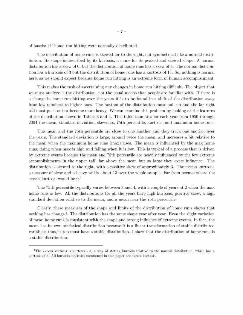
The distribution of home runs is skewed far to the right, not symmetrical like a normal distri-bution. Its shape is described by its kurtosis, a name for its peaked and skewed shape. A normaldistribution has a skew of 0, but the distribution of home runs has a skew of 3. The normal distribu-tion has a kurtosis of 3 but the distribution of home runs has a kurtosis of 13. So, nothing is normalhere, as we should expect because home run hitting is an extreme form of human accomplishment.
This makes the task of ascertaining any changes in home run hitting difficult. The object thatwe must analyze is the distribution, not the usual means that people are familiar with. If there isa change in home run hitting over the years it is to be found in a shift of the distribution awayfrom low numbers to higher ones. The bottom of the distribution must pull up and the far righttail must push out or become more heavy. We can examine this problem by looking at the featuresof the distribution shown in Tables 3 and 4. This table tabulates for each year from 1959 through2004 the mean, standard deviation, skewness, 75th percentile, kurtosis, and maximum home runs.
The mean and the 75th percentile are close to one another and they track one another overthe years. The standard deviation is large, around twice the mean, and increases a bit relative tothe mean when the maximum home runs (max) rises. The mean is influenced by the max homeruns, rising when max is high and falling when it is low. This is typical of a process that is drivenby extreme events because the mean and 75th percentile are heavily influenced by the few extremeaccomplishments in the upper tail, far above the mean but so large they exert influence. Thedistribution is skewed to the right, with a positive skew of approximately 3. The excess kurtosis,a measure of skew and a heavy tail is about 13 over the whole sample. Far from normal where theexcess kurtosis would be 0.4
The 75th percentile typically varies between 3 and 4, with a couple of years at 2 when the maxhome runs is low. All the distributions for all the years have high kurtosis, positive skew, a highstandard deviation relative to the mean, and a mean near the 75th percentile.
Clearly, these measures of the shape and limits of the distribution of home runs shows thatnothing has changed. The distribution has the same shape year after year. Even the slight variationof mean home runs is consistent with the shape and strong influence of extreme events. In fact, themean has its own statistical distribution because it is a linear transformation of stable distributedvariables; thus, it too must have a stable distribution. I show that the distribution of home runs isa stable distribution.
4The excess kurtosis is kurtosis - 3, a way of stating kurtosis relative to the normal distribution, which has a
kurtosis of 3. All kurtosis statistics mentioned in this paper are excess kurtosis.
– 8 –
6. The Law of Home Runs
Lotka, Price, Pareto and, most recently, in his wonderful book, Human Accomplishment,Charles Murray have studied the extremes of human accomplishment in literature, science, andthe arts. Murray also developed some of the statistics of sports accomplishment.
The models of these authors are power law statistical distributions of the form Prob[x] ∼ x−α.For example, Lotka’s law of the number of authors who published n works is Prob[n] ∼ C/nα.Lotka found that α ' 2 in his investigation of article publishing. Pareto’s law is also a powerlaw of the form Prob(x > k) ∼ Cx−α/k. Pareto found a value of α ' 1.5 in the distributionof income. Defining w[n] as the function representing the work done by n people, Price foundthat Prob[w(n) = 0.5] ∼ n−.5 which is to say that half the work done by n scientists is doneby a number equal to the square root of n. Price’s law is a power law expressed in terms of themedian of the distribution. Murray found that the number of PGA victories, number of victoriesin PGA majors, number of Boston and New York Marathon victories, batting championships,tennis Grand Slams, and points won in World Chess Championships are all power laws of theLotka/Pareto form. Unfortunately, he does not report his various estimates of the α values forthese accomplishments. The Lotka/Pareto/Murray laws are asymptotic approximations to theupper tail of a stable distribution, to which I now turn.
The number of home runs a player hits in a year or a career is the sum of independent randomvariables. We know that sums of independently distributed random variables converge to a stabledistribution. The normal distribution is a member of the class of stable distributions, but we caneasily see the home run distribution is not normal. We require a more general law. The generallaw of large numbers says that sums of iid random variables converge to a stable distribution. Thegeneralization from normal to the broader class of stable distributions comes from the recognitionthat the random variables need not have a finite variance or even a finite mean.
A stronger statement is this: the distribution function F possesses a domain of attraction ifand only if it is stable. The limiting distribution function of independent r.v.’s Xk belongs to thedomain of attraction of F if there exist normalizing constants an, bn > 0 such that the distribution of(∑n
i=1 Xi−an)/bn → F. Thus, we might expect that extraordinary accomplishment might convergeto a stable distribution because it is, in some sense, unlimited in the amount by which a singularaccomplishment might exceed others. This is the intuitive meaning of the infinite variance and ofthe possibly infinite mean.
The Normal (Gaussian) distribution is stable (as it must be because it is the attractor of sumsof random variables), but it is the only stable distribution with a finite variance. The Pareto,Levy, and Cauchy distributions are the other (named) stable distributions. But, there are manyother members of the stable class, whose functional forms cannot be given. Since they do not havespecific functional forms, they must be expressed through the more general characteristic function.
Levy (Levy 1954) characterized the class of stable distributions through their characteristic
– 9 –
functions. A stable distribution X ∼ S(α, β, γ, δ) is a four-parameter distribution with character-istic function given by
Estimation of the stable distribution of home run hitting produced values of the parametersshown in Table 1.5
Table 1: Maximum Likelihood Estimates of the Parameters of the Law of Home Runs
α β γ δ
Index Skewness Scale Location Log-LikelihoodHome Run Hitting
α-stable 1.6422 1.00 6.219 12.30 −39294.2
The exponent α is a measure of the probability weight in the upper and lower tails of thedistribution; it has a range of 0 < α ≤ 2 and the variance of the stable distribution is infinite whenα < 2. The basin of attraction is characterized by the tail weight of the distribution (α). Thisremarkable feature tells us that the weight assigned to extreme events is the key distinguishingproperty of a stable probability distribution. The skewness coefficient −1 ≤ β ≤ 1 is a measureof the asymmetry of the distribution. Stable distributions need not be symmetric; they may beskewed more in their upper tail than in their lower tail. The scale parameter γ must be positive.It expands or contracts the distribution in a non-linear way about the location parameter δ whichis the center of the distribution.
The tails of a stable distribution are Paretian and moments of order ≥ 2 do not exist whenα < 2. This is typical of many extraordinary accomplishments, as seen in the works of Lotka, Pareto,and Murray. Its mean need not exist for values of α < 1. When α = 2, the stable distribution isthe normal distribution with a finite variance. The parameter α is called the tail weight because itdescribes how rapidly the upper tail of the distribution decays with larger outcomes of the randomvariable; smaller α implies a less rapid decay of probability.
The distribution of home runs is skewed to the right with a value of β = 1.00. The probabilitydensity function is shown in Figure 4. Note the peak probability (mode) is well to the left at 7.8home runs; this is the statistically most common number of home runs by a player in a year. Thefit to the data is remarkable as shown by the cumulative theoretical and empirical distributionsdisplayed in Figure 5.
5I used Dr. Robert Rimmer’s Mathematica package to estimate the parameters of the stable distribution. It is
described in the Mathematica Journal (Rimmer and Nolan 2005).
– 10 –
Its central mass is located at δ = 12.3., just above the average. The important tail index isα = 1.642. Since 1 < α < 2 the distribution has a finite mean but an infinite variance. This reflectsthe large probability mass that is located out in the right hand tail. It is a warning that we cannever sample the whole distribution so our experience does not inform us of the events that arepossible. And the infinite variance implies that predictions lack any precision; a prediction thatplayer Z will hit K home runs next season, plus or minus infinity is no prediction at all.
Some other diagnostics are in order. First, consider the change in home run hitting by takingeach player’s home runs for each year and then taking the first difference. Figure 6 shows thechange in home runs for each year of the sample. There is no change; the series is centered onzero and has no drift whatsoever. In fact, the largest positive deviation in home runs is by RogerMaris in his record year of 1961. Mark McGwire’s record of 70 in 1998 is the next largest positiveleap. Leaps and falls are pretty evenly divided, there are 5 players above a positive change of 20home runs and 6 players below a negative change of 20 home runs. Barry Bonds leap in his recordyear is exceeded by Maris and McGwire and matched by 7 other players in other years. Nothingso unusual here.
The changes are fairly extreme among players, but there is no trend at all. The kurtosis of thedistribution of changes is large, 7.98, meaning the distribution is far from normal. It shows moreextreme deviations than would be true if home run hitting were normally distributed. The meanchange is zero, with a standard deviation of 10.03. The frequency distribution of changes in homeruns hit by players is almost a classic picture of a stable distribution, with a narrow, high centralpeak and long tails; see Figure 7.
7. Home Run Records
What about home run records? As the perevious section demonstrated, home run hitting is a“wild” process. But, it has features that are regular too. Both of the distributions of the numberof home runs by players and the change in home runs are far from normal. Hard things neverare normal. Both processes follow a Paretian Stable distribution and have infinite variance. Thechanges are stationary over time but they have a large variation and the variation tends to cluster,like volatility in markets.
The most home runs hit in a season will have less variability than home runs. The maximumorder statistic is known to follow a generalized Pareto distribution. A generalization of this distri-bution is the Stable Paretian distribution whose parameters are estimated in Table 2. It is a lessskewed distribution than the distribution of home runs itself and has a smaller scale, but is locatedmuch farther to the right at 47.77 home runs. Its tail weight α is almost the same, 1.56 as the 1.64for home runs.
The time series of MLB leading home runs shown in Figure 8 is rugged, with leaps and valleys,and there is no trend. There is a leap in Roger Maris’ 1961 record year and then leaps in three
– 11 –
Table 2: Maximum Likelihood Parameter Estimates of the Distribution of League Leading HomeRuns
α β γ δ
Index Skewness Scale Location Log-LikelihoodHome Run Hitting
α-stable 1.5659 0.7049 4.1548 47.7713 −156.73
other years of 1998, 1999, and 2001. The low of 31 is two standard deviations below the mean of48 and the high of 73 is just under three standard deviations above the mean. These are samplestatistics, the standard deviation of the distribution does not exist because α < 2.
8. Measuring Home Run Effectiveness
We now have ample warning that the distribution of home runs is a “wild” distribution thatthrows “normal” analysis out the window. But there are still some things we can try to discoverin terms of hitting strategy and effectiveness of modern players over old timers. Maybe they arestriking out more often and hitting more home runs because they are “swinging for the fences.”Maybe they are more powerful in some measurable way.
Perhaps the purest measure of power hitting is home runs per hit. This takes base on balls,at bats, number of games played, hitting average and other factors out of the measure. With thatsaid, I also develop the numbers for home runs per at bat since this may be both an attribute ofpower and an indicator of strategy. As a measure of home run efficiency, I also consider home runsper strike out. I consider home runs per strike out to be a strategic variable as well as a measureof skill and power. If a player is trying to hit home runs, he will strike out more often. If he is notskilled or powerful, the hard swings will not produce results and he will have few home runs perstrike out. Some players change their strategy over time as they gain skill and mature. Strike outs,home runs per hit and per at bat, and home runs per strike out give us a sense of their strategyand effectiveness.
It turns out that all these measures have the same kind of skewed, heavy tailed distributionsthat we have already encountered. Seeing the same shape once again is a powerful confirmation ofour finding that home run hitting is an stable Paretian distribution because this implies that anyway you look at the process you should that the distribution has the same shape.
Table 5 summarizes the statistics of home runs, home runs per hit, home runs per at bat, atbats per player season, base on balls per year, strike outs and home runs per strike out. It is usefulto look at these statistics before we look more closely at the players who produce them. Noneof these variables follow a normal distribution according to standard tests. In addition to these
– 12 –
distributional statistics, I have tabulated the annual figures by year of these variables for all hitterswith 200 or more at bats from 1959 through 2004. The tabulations appear in Tables 6, 7, and 8.The data cover 45 years and 11992 player years.
Home runs per hit has a mean of .101, a large standard deviation (relative to the mean) of .07,positive skew and excess kurtosis. It reaches slight peaks in the 1960s, in 1987, and in the 2000s.The least value for a player is 0 and the most is an astonishing .52. Even a value as low as .29 isin the 99th percentile. The median is below the mean another indicator that the probability tailto the right is heavy.
Home runs per at bat (which does not count a walk as an at bat) have a mean of 0.027 anda large standard deviation of 0.019. The median is below the mean and the skew and kurtosisstatistics verify that the distribution has a peak to the left and a long tail to the right, truncatedat 1.
At bats per player is rather stable, partly because I have considered only players with 200 ormore at bats. It is near its long term average of 416 at the beginning and end of the 45 years ofthe data. Base on balls is also rather stable.
Strike outs tell a different story. They begin to increase to more than 70 strike outs per gamebeginning in 1996 and remain above the long run average of 64 strike outs per game through 2004.Modern hitters strike out more than the old timers (even Ruth only averaged 68 strike outs), inspite of the smaller strike zone (see below). Their home run efficiency per strike out is a bit lessthan it was in the 1960s and right at or just above the long run average of 0.18 home runs perstrike out. More strike outs and less home run efficiency per strike out suggests a strategic changein baseball in the mid nineties toward the long ball.
Home runs per player have drifted up a bit, but we now know that this average is dominatedby the elite home run hitters. And, we know that the mean is volatile and should vary accordingto the law of home runs. Home runs per hit have hardly changed over the years; home runs per atbat are remarkably stable, and home runs per strike out are only slightly above the long run meanin the latter years, but still lower than in the 1960s. Nothing has changed.
9. MLB Home Run Production
Now the question becomes what is the source of the slight change in total home runs hit inthe major leagues over time? Has home run production increased at all levels of hitting in the bigleagues? Or is it a few premiere hitters? Here are some things to think about.
I graphed home run hitting in percentiles over the time period of 1959 to 2004 in Figure 3. Thefigure shows home runs per hit in the 20th, the 50th, the 70th, the 90th percentiles of all hittersand the most home runs hit in a year by a single player. Only the maximum shows a peak duringthe McGwire, Sosa, and Bonds great years. Otherwise, there is no trend toward a higher number
– 13 –
of home runs per hit over this long time period. Even the 90th percentile hitters did not exceedslightly more than 0.20 home runs per hit, nowhere near the levels attained by a few, unique powerhitters, and their production is unchanged over time. Even the 90th percentile hitter looks like anunderachiever compared to these guys.
Many changes in the Major Leagues have taken place over the many years of the hitting dataI have analyzed. The season has lengthened from 154 to 162 games per year. The number ofteams has grown from 16 to 30. There have been 4 player strikes with shortened seasons. Therehave been changes in ballparks, modest changes in bats, and allegations of a change to the ball.The American League adopted the designated hitter in 1973. In addition, the players have betterhitting mechanics and train for power. To quantify the effects of these changes, I have developeda simple empirical model of the total home runs hit in MLB each year.
The model of annual MLB home run production is:
HR = β0 + β1teams + β2games + β4maxhr + ε
The estimates of the model are in Table 9. I have used maximum likelihood estimates ofthe general linear model because the error term is not normally distributed. Nonetheless, theseestimates differ little from the least squares estimates where the model accounts for about 83 percentof the variation in the data.
What do these results indicate? The coefficients are all estimated with small standard errors.The teams coefficient indicates that adding another team to MLB adds 115.56 home runs to averageMLB home runs per year. An additional game (mlbg) increases average home run output by 1.08.The variable maxhr is the most home runs hit in the year by a player. This variable captures theeffect of the extreme performances on the league total. A one unit increase in the number of homeruns hit by the league-leading hitter raises total MLB home runs by 49.11. This is remarkable.It suggests some kind of home run competition among players of the sort that went on betweenRoger Maris and Mickey Mantle in 1961 or Sammy Sosa and Mark McGwire in 1998 and 1999. OrSammy Sosa and Barry Bonds in 2001.
But it goes beyond that to suggest that Ken Griffey (56) and other players may have beencaught up in the contest and hit more home runs too. Hitting home runs is more than a matter ofpower, it depends on strategy. On the third strike, for example, some players try to put the ballin play rather than go for a home run. Swinging harder and/or with a slight upper cut is anotherway to alter hitting strategy. A player may see others hitting home runs and begin to train andpractice more effectively. The size of the coefficient, 49 more home runs in the league when theleading hitter hits one more, is some evidence that players follow the leading home run hitter or tryto surpass him. It is said that when Honus Wagner saw Babe Ruth hitting home runs he alteredhis hitting and increased his home run output from less than 10 a year to 40 a year.
– 14 –
10. Self-similarity and Intermittence
The Paretian upper tail of the stable distribution law of home runs has two intriguing prop-erties. The probability distribution is self-similar, meaning that parts of the distribution look justlike the whole. If you look at the distribution through a narrow window or a broad one, you willsee the same distribution. For example, estimating the stable distribution far into the upper tailbeyond 50 home runs (the top 0.15 percent of home runs) also yields a stable distribution with asimilar tail coefficient of α = 1.535 and an appropriately rescaled location value of δ = 58.58. Inthis region, you see the pure Paretian tail. The distribution has the same shape, the crucial featureof self-similarity.
The Richter law of earthquakes is a Pareto or power law distribution.6 It says earthquakes ofall sizes may occur and there is no typical earthquake. The law of home runs says the same thing;there is no typical home run year in baseball or typical home run hitter either. Earthquakes cancome in bursts and there can be longer intervals of calm. The number of quakes per day, week,month, or year is random and they have the same distribution (similarity again). There is somelonger term correlation between quakes. So, earthquakes can come in clusters and bursts of allsizes. They are not spread out like margarine on bread, all even and smooth.
That is the nature of the wild statistical distributions that describe earthquakes, storms andrainfall, disasters, stock markets (where there is evidence of volatility clustering), and home runs.They are all “bursty” processes and, according to the law, the size of fluctuations is greater amongthe most prolific home run hitters. This is apparent in Figure 3 where the maximum home runs perseason is more volatile than the 90th and lower quantiles. This is not an anomaly. It is implied bythe law of home runs; a power law tail implies that fluctuations increase with higher rank (Sornette2000). So clusters of events occur, they have no typical size, and the fluctuations are larger amongthe best home run hitters. Thus records are made and fall in an unpredictable and intermittentmanner. The burst of home run records in 1998 through 2001 is well within our expectation fromthe statistical law of home runs. There is no need for recourse to an external cause like steroids toexplain it. This cluster of records looks very much like the cluster from 1921 to 1927.
11. A Closer Look at Palmeiro, Bonds, Sosa, and McGwire
Because of his suspension and status as a home run hitter I look more closely at RafaelPalmeiro’s career (see the Appendix: Table 10. He began play in 1986 with 3 home runs in 73 atbats. In all his succeeding years he appeared at bat more than 200 times, commonly he appearedin from 400 to 600 at bats. The increase in his at bats reflects the expansion of the number of
6The upper tail of the distribution of home runs is a power law distribution that is known to be scale-free and
subject to bursts or avalanches (Bak and Chen 1991). See William Brock (Brock 1993) and Schroeder (Schroeder
1990) on power laws, flicker distributions and intermittence.
– 15 –
games per season and his durability as a player.
His peak home runs per hit, per at bat, and per opportunity occurred in 1999 and 2002 whenhe hit 47 home runs in 565 and 546 at bats respectively. He averaged 531 at bats through hiscareer. This high average has been an important part of his productivity as a home run hitter.His average of 29 home runs per year is well above the MLB average of 11.7 for players with atleast 200 at bats. His strike outs are average, but they did peak during his prime home run years;by 1996 he was striking out at least 90 times when he had at 600 at bats or more. His home runefficiency was highest in 1995 (37 home runs) and in 1999 (47 home runs), exceeding .60 in eachyear. In his other big year in 2001 with 47 home runs, he managed to have 600 at bats with 90strike outs, with a home run efficiency of 0.52.
There is no break or jump in Palmeiro’s home runs per hit, the most reliable measure of power,anywhere in the series. His most powerful years were from 1995 through 2003, when he exceeded0.21 home runs per hit. He hit more than 37 home runs ten times in the stretch from 1993 through2003, with a drop to 23 in 1994, a year in which he had only 436 at bats. His peak years of 47 homeruns are one standard deviation above his long run average. 2004 was one of his least productiveyears as a power hitter, just 23 home runs in 550 at bats and a home run efficiency of only 0.38 alevel he hit in 1991 and that he had exceeded every year but one since 1993. If he used steroidsduring the year, there is scant evidence that it was effective.
In the Appendix in Tables 11, 12, 13 I also do the same tabulation for Bonds, Sosa, andMcGwire. Bonds has the highest home run average of 37 and, by far, the largest number of baseon balls of 121 per year. His average 478 at bats per season trails Palmeiro by about 50 but isjust ahead of Sosa at 471 and far ahead of McGwire who only averaged 363 at bats per season.McGwire and Sosa are tied in home runs per year at 34, ahead of Palmeiro, but behind Bonds.Sosa and McGwire had to hit more home runs per at bat and per hit to come so close to Bonds’hitting because they had fewer at bats than he during these years.7
In his record year of 2001, Bonds had the most strike outs of his career since 1989. His homerun efficiency was a high 0.78. He was swinging for home runs and did it well. But, in 1994 he hada higher home run efficiency equal to 0.86, but so few at bats that he hit only 37 home runs. By1993 his home runs per at bat were beginning to reach Ruthian levels. He hit 0.09 home runs perat bat that year and kept it near or above that level since. By 1999 he broke into the magic 0.30or more home runs per hit to stay (he had previously done it in 1994). From 2001 through 2004,he exceeded even Ruth in home runs per hit. His at bats and strike outs decline dramatically from2001 onward. But, he didn’t have as many big years as The Babe, just one huge year and thensome good ones.
Sosa has always been a free swinger, striking out an average 124.12 times a year and more than170 times three times. That is one reason why he hit more home runs than anybody in MLB from
7Now Bonds’ at bats are among the lowest because his is walked so often.
– 16 –
1996 through 2004 when he hit an average of 49.22 home runs a year. His home run efficiency islower than Palmeiro’s or Bonds’, but for him the strike out home run trade-off was very favorable.They pay you for home runs not for avoiding strike outs and he hit more than anybody during hisbest years.
McGwire had a stunning streak from 1995 through 2001 in which he hit 0.4 or more homeruns for every hit. But, in only two years did he hit more home runs than he hit in 1987 (52 isessentially a tie with 49 from a statistical point of view). His record year in 1998 of 70 home runs istwo standard deviations above his average. 1999 is about one and three quarters above his average.Yet, in neither of those years does he match his home runs per hit of 2001. His record years of1998 and 1999 coincide with over 500 at bats, a figure he previously attained only three times earlyin his career. In contrast, Bonds, Sosa, and Palmeiro appeared at bat more than 500 times manytimes in their careers, though Bonds’ at bats in his last two years were hampered by many walksand fell below 400. McGwire was clearly swinging for home runs in his big years of 1998 and 1999;his strike outs jumped far above his average to 155 and 141 respectively.
Finally, let us compare these players to home runs hit in the past. In Figure 9 we see the mosthome runs hit each season in MLB and the number of home runs hit by Sosa, McGwire, Bonds.The league-leading home run series is centered at the mean of 48, with peaks and valleys throughthe years. Maris’ record is at the 90th percentile, McGwire’s is at the 95th and Bonds’ record is atthe 99th percentile. The distribution is not normal and it has a narrow central peak with a long,heavy tail to the right. These are the classic signs of a Paretian or more general stable distribution.
In their best home run years, all these players were clearly going for it and paying the smallprice of more strike outs. They had high home run efficiency. McGwire’s home run efficiencypeaked in 1995 at 0.51, but it was already at 0.47 in 1993. Bonds peaked at 1.10. Palmeiro peakedat 0.68 and Sosa at 0.42. These guys are far above other players who have an average efficiency0.176.
12. The Baseball, Ball Parks, The Strike Zone, Bats, Players, and Steroids
We have to go over a few of the many explanations that have been offered for an increase inMLB home runs. As we should expect, they do not stand up to scrutiny because there have beenno fundamental changes.
The Baseball The coefficient of restitution of the baseball was increased in 1920, making itrebound off the bat with higher velocity. The number of games increased from 140 to 154. Thatyear, Babe Ruth hit 54 home runs, breaking his record of 29 from the year before. So, he benefitedfrom a hotter ball and more games in breaking his record.
In the modern era, claims persist that the ball has been made hotter off the bat. If it were
– 17 –
lighter or had more rebound, the effect would be to increase home runs. Yet, there is no evidenceto support this claim. Each time it is tested it is rejected.
In response to a controversy about the “hot” 1977 baseball, it was tested against the 1976 ball.The 1977 ball rebounded 1.3 percent higher in a small sample of balls tested. This is well within therandom variation among baseballs; the MLB standard permits a variation of 3.2 percent. Anothercontroversy concerned the 1999 and 2000 baseballs. Tests again showed there was no difference. Dr.Jim Sherwood’s measurements confirm that the 1999 and 2000 baseballs have the same coefficientof restitution (COR). A test of balls a decade apart, of 1988 and 1998 baseballs, by R. C. Larsenshowed no difference (Adair 2002).
Current MLB standards set a rebound velocity of 54.6 percent of the speed of the ball at impact,plus or minus 3.2 percent. Weight and COR variations among balls could cause two conformingballs, one light and hard, and the other heavy and soft, to differ by as much as 49 feet distancewith the same impact. It also is true that balls are no longer used as many times in modern MLB.Impacts and scuffs can alter the ball flight and lower the COR.
The baseball is smoother say umpires such as Mike Reilly (Kaat 2000). Testing by Jim Kaatand Popular Mechanics showed that 2000 MLB baseballs were slicker than 1999 baseballs; they hada slightly lower coefficient of friction. There were no differences, however, in batted-ball speeds. Asmoother ball will travel a shorter distance because it does not break the airflow into a turbulentflow where resistance drops (Adair 2002). On the other hand, the test showed that the seamswere a bit higher on the 2000 baseball, but this may have been a matter of the sampling andmeasurement. Higher seams would break the airflow and make the ball travel farther as its airflowbecomes turbulent. A smoother ball may also move differently when thrown by the pitcher; thelate-breaking cut fast balls and back-up sliders that are thrown today may not have been possibleyears ago. A slicker, harder-thrown ball will break later and a ball with higher seams will breakmore. On the whole a smoother ball with slightly higher seams would probably be of more benefitto the pitcher than the hitter.
In short, aside from the change to the baseball in 1920 there are no confirmed tests that showany other changes of significance in the baseball. But, with each apparent surge in home runs, andI stress apparent, people seem to look for an explanation. Tests from 1976 to 2004 indicate thatthe baseball has not changed in a way that would permit more home runs to be hit.
Ball Parks The House that Ruth built, Yankee Stadium, opened in 1923 and was suited to hishome run stroke. Only 295 feet down the right field line and 350 to short right center to a pull hitterlike the Babe must have been a very friendly hitting environment. Maris, who broke the Babe’srecord in 1961, was also a left-handed hitter and he set his record playing home games in YankeeStadium. Hank Greenberg came close to the record by hitting 58 in 1938. He was a right-handedhitter playing in a not-so-home-run-friendly Briggs Stadium which was 340 feet down the left fieldline and 365 to left center.
– 18 –
The only rigorous research on ball parks shows that the average of the required ball velocitiesto hit a home run the park dimensions (left field, left center, center, etc.) of MLB parks varies little,from a ball velocity off the bat of 107 to 110 feet per second. There is no comparable historicalanalysis that would permit a conclusion as to the effects of the various dimensional changes thathave taken place in MLB ball parks over the years.
One change that in ballparks that might boost home runs is the addition of Denver to majorleague baseball. The high altitude and low air density allow a struck ball to carry farther thana sea level. Atlanta is located at a higher altitude too. But, the addition of other parks at lowaltitude, such as Miami and Houston, seem to have offset Denver and Atlanta, leaving a only asmall net change in average park altitude.
The Strike zone The strike zone has gotten smaller. Whereas the height of the strike zone wasthe top of the letters or the arm pits, it has moved down to half the distance between the shouldersand the belt.
Both Barry Bonds and Babe Ruth are 6-ft.-2in. in height. With a 17-in.-wide plate, BabeRuth had a strike zone of roughly 545 square inches. In 2001, Barry Bonds, had a strike zone ofabout 410 square inches. The high fast ball at the letters that used to be a strike out pitch is notavailable to pitchers in recent years. In spite of the shrinking strike zone, strike outs per playerhas drifted upward over the years (see Table 5) from 56 per player in 1961 to 77 in 2001. Swingingfor the fences does seem to produce more home runs and strike outs. Remarkably, home runs perstrike out are down from 0.23 home runs per strike out in 1961 to 0.19 in 2001. Modern hittersare a bit less efficient than players of the 1960s in hitting home runs. This suggests they really areswinging for the fences because the smaller strike zone should have increased home runs hit perstrike out.
The smaller strike zone may be an explanation for the very slight upward drift in the numberof at bats players get per game; it has increased by 0.6 at bats per game.
Bats MLB rules governing baseball bats have not changed. Bats must be made of wood and thebarrel of the bat must not exceed 2.75 inches in diameter. Earlier bats tended to be made fromhickory. Ash became more common later and is the main wood used in bats today. Maple is usedby a few players. Maple is the denser of these woods, followed by hickory and then ash.
Babe Ruth used a hickory bat weighing 47 ounces to hit 60 home runs. A bat of that sizehad a full 2.75 inch barrel. Roger Maris used an ash bat weighing 33 ounces to hit 61 home runs.Barry Bonds used a maple bat weighing 33 ounces to hit 73 home runs. To make a bat as lightas 33 ounces, it has to have a smaller barrel diameter. Consequently, the ash bat Maris used andthe maple bat Barry Bonds used had a barrel diameter of just 2.50 inches, a loss of hitting area ofabout 4 percent (Adair 2002). Henry Aaron hit more home runs than anyone with a bat weighingfrom 31 to 32 ounces.
– 19 –
A heavier bat will hit the ball farther if it is swung at the same speed as a lighter one. Sincethe kinetic energy is mass times velocity, there is a trade off between bat speed, weight and power.Modern players, facing a large variety of pitch speeds from 70 mph change ups to 98 mph fastballs,use lighter bats than players of the past. A light bat will actually drive a slower pitch farther thana heavy bat. A light bat gives the hitter a few milliseconds longer to judge a pitch, but its maincontribution may be in the higher precision of the swing path. Home runs are hit by striking theball about half an inch below center, generating lift and back spin. Mammoth home runs must belaunched at around 35 degrees. So a slight upswing and a strike just below center are optimal forhitting home runs (see (Williams 1986) and (Adair 2002)).
Players Babe Ruth was 6’ 2” inches tall and weighed 251 pounds when he hit 60 home runs in1927. He was quite a bit more massive than the typical MLB player of the time. Mark McGwirewas 6’ 5” and weighed 225 when he hit 70 home runs in 1998. Barry Bonds was 6’2”, like Ruth,and weighed 220 pounds. Sammy Sosa is 6’0” and also weighs 220 pounds. Home run hitters aremore massive than the typical player.
With the same bat speed, a heavier player will generate more energy to drive the ball. In hisPhysics of Baseball Dr. Adair (Adair 2002) shows that total energy is approximately proportionalto player weight. A 140-pound player swinging a 32 ounce bat would drive a 90-mph fastball 338feet, a long out or off the fence if pulled down the line in most parks. A 225 pound player swingingthe same bat at the same speed would drive the ball 382 feet, a home run to all but deep centerin most parks. A more massive player can also swing a heavier bat, which adds to distance. But,the strong qualifier is that the bat must be swung at the same speed and a heavier player may nothave the same quickness to accelerate the bat as a lighter player.
If there were more home runs in MLB, an explanation could be found in the mass of themodern MLB player. Modern players are larger than players of even as few as 30 years ago, just asthe current generation of Americans is taller and heavier than previous generations. On the otherhand, it is more difficult for a larger player to put the fine kinetics of a beautiful and powerfulswing together or to react and accelerate the bat quickly. If size were all that mattered, baseballplayers would look like NFL football players. Longer limbs make for longer levers that are moredifficult to move accurately and quickly.8
Steroids At this point, there is nothing left to explain and no need to invoke any external sourcesuch as steroids for MLB home run hitting. There have been no changes in home run hitting. Thatshould be the end of it. But, it isn’t. Records have fallen and for the critics of baseball there mustbe an explanation, a cause. And they seem to have the explanation they seek in steroids. Let’s
8A 6’4” in height, Ted Williams (Williams 1986) kept his hands very close to his body in his hitting stance,
stressing the quickness that gave his swing.
– 20 –
look at the argument and some facts.
First, there is no causal explanation required for home run records. Under a random process,the realizations of the events just happen. Explaining why you drew a Spade instead of a Diamondwhen the draw is random is silly. No explanation is required; it is a realization of a random process.
Home run hitting is one of the most random and uncertain of human activities. The law ofhome runs has an infinite variance, which is about as uncertain as anything can be. That meansthere is no basis for anyone to say how long records ought to last or how often they should bebroken. We have only probabilities. And just as you can get three or five heads in a row in a seriesof coin tosses, you can get clusters of home run records. It is nothing more than a random seriesof events. No more explanation is required for home run records than for three heads in a row.Under the law of home runs, new records have non-vanishing probability, far more than one wouldexpect if they were thinking in terms of averages and normal distributions. The probability of newrecords is far higher than a normal distribution would make possible.
Steroid advocates have to argue that the new records are not consistent with the law of homeruns, that the law itself has changed as a result of steroid use. They have to show that the Sosa,Bonds, and McGwire performances are impossible under the statistics of home run hitting. But,this is not true. The cluster of recent records is perfectly consistent with, and even implied by, thestatistics of home run hitting. It also is consistent with bursts of home run records in the past.
There are two other hurdles the steroid hypothesis must clear. One must show positive proofof steroid use by a record setting home run hitter and, further, that steroids are the cause. There isslim evidence on the first score. We should note that only 9 players have been suspended for testingpositive for steroids in thousands of tests; approximately 3990 players were in the big leagues overthe past three years. That is only a positive rate of 0.002. The test surely has a false positive ratehigher than that. And there are contaminants in most supplements that nearly all players takethat would cause them to test positive even if they are not taking steroids.
As to steroids themselves, they are highly overrated as aids to home run hitting. McGwire,Ruth, Maris, Sosa and Bonds rarely hit balls to the warning track. When they connected the ballswere gone, far over the wall. This was true throughout their careers. Bonds and Maris were linedrive hitters earlier in their careers, but once they developed as home run hitters (a home run hitterswings slightly upward to launch the ball at a 35 degree angle and hits the ball just below center asopposed to a line drive hitter who has a level swing and hits the ball in the center) their home runslanded in the seats, not on the warning track. Were steroids effective at increasing bat speed (andthey have not been shown to), they could increase home runs by lengthening warning track hits by10 to 20 feet. Dr. Adair estimates that about 1 hit lands on the track for every 10 home runs. ForRuth, Maris, et al far fewer balls land on the track for every home run they hit. Suppose it is 1out of 25. This means that, at most, higher bat speed would increase home runs by 1 to 3 a yearin these great hitters. So, the test of steroids would be to calculate the number of warning trackhits relative to home runs for a known steroid user and show that what were previously warning
– 21 –
track shots become home runs. No one has produced this evidence.
But, even that may not be good evidence, because there are no strong reasons why steroidsshould increase bat speed. Steroids encourage hypertrophy in body builders and strength athletes,who use massive amounts, train long and hard, and do very high volume work. No baseball playercan afford to train that long and the training would be highly counterproductive to his baseballplaying. Body builders and strength athletes (power lifters) are not particularly quick. While thereis evidence that steroids increase muscle mass of body builders and strength athletes, this musclehypertrophy will not increase the important fast twitch muscle fibers that home run hitters rely on.Body builder and strength athlete exercises produce a higher volume of slow twitch muscle fiber,the antithesis of rapid power production.9
Hitting an 85-mph pitch 400 feet requires a bat velocity of 70 mph. The bat must be acceleratedto this velocity in 200 milliseconds. Such a feat requires rapid force generation that can only besupplied by fast twitch muscle fibers. Body building, and the slow twitch fiber composition that itproduces, could not produce the power and speed that Mark McGwire, Barry Bonds, and SammySosa exhibited in their prime years. Speed strength is developed using rapid movements that do notresult in hypertrophy. And there is no evidence that steroid use directly promotes speed strength.Even these modern players are not as muscular as Ted Kluszewski or Steve Bilko were in theirprime. In fact, they look like slightly taller versions of Mickey Mantle, a densely muscled player ofthe past.
Again, The Babe has the final word on steroids. The last home run he hit, number 714, inhis last game in 1935 with the Boston Braves in a season of just 72 at bats, was one of the longestof his career. Using a 36 ounce bat, he hit the first home run ever hit over the right field roof ofForbes Field in Pittsburgh.10 Films show that he was a shadow of his former self by this time andhe likely already had the cancer that would kill him a 13 years later.
Other long home runs from earlier years show that the longest home runs have not changed.Hank Greenberg in 1938 and Vic Wertz in 1948 hit balls that were caught in center field at morethan 450 feet. Joe Adcock, Lou Brock, Hank Aaron, and Luke Easter all hit home runs over thenine-foot screen in front of the center-field bleachers 480 feet from home plate in the Polo Grounds.Mickey Mantle hit a ball out of Griffith Park in 1953 that is estimated reliably to have gone 506feet, aided by a 20-mph wind (Adair 2002). Dick Stuart hit a home run over the 457 foot left-centerfield corner of Forbes Field in 1957.11 These home runs are comparable to any hit today.
9The literature on highly hypertrophied body builders demonstrates slower contraction/relaxation speeds and a
muscle fiber shift away from the fastest type IIx/IIb muscle fibers toward slower fast twitch type IIa and even the
slow twitch type I muscle fibers. See the review by Angus Ross and Micheal Leveritt (Ross and Leveritt 2001).
10Right field was 300 feet down the line and 375 to right-center. The roof was 86 feet high. Only 10 players have
duplicated the feat since, Mickey Mantle, Eddie Mathews, Willie McCovey, and Willie Stargell among them. Thanks
to Michael Stima for this information.
11The ball was estimated to land 500 feet from home plate. Michael Stima, personal communication.
– 22 –
Home Runs per Game The measure that many proponents of the steroid explanation seem topin their theory to is home runs per game. This reasoning is flawed. First, home runs per gametell us nothing about records. Records are about extreme performance, not some kind of average.Records are made by extraordinary performances that have no relation to average home runs pergame.
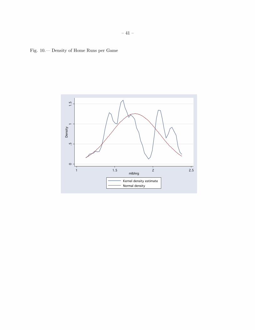
Second, home runs per game is a strange statistic. Home runs per game is simply total MLBhome runs divided by total MLB games. Why should this almost meaningless calculation be awell-behaved measure of performance? It turns out to have a strange statistical distribution thathas four peaks (two to the left of the mean and two to the right) and a deep valley just abovethe mean. The density in shown in Figure 10 where I have overlaid the normal distribution forcomparison. It is far from normal, it is multi-modal, left skewed (skewness of 0.19) and has morekurtosis (1.91) than a normal distribution. It is a monster that cannot be used to set a standard.
If you think for a moment about the constraints of a ball game, it becomes obvious that homeruns per game cannot be a well-behaved statistic that can be used to make sharp comparisons. Thenumber of home runs in a game is an integer, not a continuous variable. The number of leaguegames is an integer too. Dividing these numbers will give rational numbers, but they will not bedistributed normally and will have strong modes at a few typical values. The progression of a gamesets constraints on home runs. If one home run is hit, the odds that two will be hit go up. And iftwo are hit, the odds that three will be hit go up. And so on. But, as more home runs are hit in agame, the odds that greater numbers will be hit decline because innings and at bats run out.
No valid comparisons can be made using MLB home runs per game.
13. Conclusions
Why do all the attempts at explaining an increase in MLB home runs seem to fail? I think it isbecause they are attempting to explain something that has not happened. There are no more homeruns in baseball than before when the problem is properly analyzed. Once the number of gamesand other variables are factored into home run productivity and the random nature of home runhitting is taken into account, there is no change. That may be why all the attempts at explanation,such as steroids, hotter balls, altered strike zones, and home-run-friendly ball parks fall apart whenthey are tested.
Many sportswriters and fans make two mistakes. One, they think home runs have increasedwhen they have not. I show here that the probability distribution has not changed. And, two, theythink a random event, such as a new record, calls for some kind of external explanation. The newrecords are completely within the variation of outcomes under the stable probability law of homeruns. You do not need an explanation for a random event when you have evidence that the law ofhome runs has not changed in 40 years. If you roll box cars three times in a row do you require anexplanation? Only people who fail to understand chance do.
– 23 –
The same law of home runs holds now that held 40 years ago. Year to year differences inhome runs require no explanation; they are all within the variation of the outcomes under thestable probability distribution of home runs. The burst of new records does not require an externalexplanation; they are part of the pattern that comes from the nature of the law of home runs.People often look for an “explanation” of purely random events. Looking for a “hotter ball” orsteroids as a cause of a random event is just another example of the human failing to understandchance and randomness.
The pace of new records in recent years is due to the extraordinary accomplishments of threeprodigious hitters. We have lucky enough to see three Babe Ruth’s in this generation. Hitters suchas these may never appear again. You cannot take an ordinary player and turn them into homerun hitters of the accomplishment of Bonds, McGwire, and Sosa by dosing them with steroids. Itmay even be harmful. Home run hitting of that magnitude is as incomparably rare as the greatestworks of science or art.12
It took more than 80 years and more than 100,000 player-years of baseball for 5 home runhitters of the caliber of Ruth, Maris, McGwire, Sosa, and Bonds to appear. We have been luckyenough to witness three of them in the past few years. To diminish their accomplishments onthe basis of speculations and rumors about steroids, as members of Congress and the media havedone, has the facts and the science wrong and is profoundly ignorant of the statistical laws ofhuman accomplishment. McGwire, Sosa, and Bonds are home run geniuses, not ordinary hitterson steroids; they are the Bach, Mozart, and Beethoven of home runs.
Will another player of the prowess of Babe Ruth, Roger Maris, Mark McGwire, Sammy Sosaor Barry Bonds ever appear again? Even greater performances are possible because the law ofhome runs has a long Paretian upper tail with positive and non-vanishing probability mass. But,the chances are small. The law of home runs says that the probability that Babe Ruth’s record of60 home runs would be broken is 0.0109. Given more than 100,000 tries in nearly 80 years, it wasalmost sure to fall. Barry Bonds’ record of 73 will be harder to break. According to the law ofhome runs, the probability that his record will be broken is 0.007206.
12Even Shakespeare had his doubters; there was a long controversy over his extraordinary works that led some
scholars to contend that no one person could have accomplished what he did. The claim circulated that Francis
Bacon must have written some Shakespearan plays. Maybe Shakespeare was on steroids.
– 24 –
REFERENCES
Adair, R. (2002). The Physics of Baseball. HarperCollins, New York.
Bak, P. and Chen, K. (1991). Self-organized criticality. Scientific American, 264(1):26–33.
Brock, W. A. (1993). Scaling laws for economists. Technical report, University of Wisconsin,Madison.
De Vany, A. (2003). Hollywood Economics: How Extreme Uncertainty Shapes the Film Industry.Routledge, London.
Kaat, J. (2000). Baseball’s new baseball. Popular Mechanics.
Kiele, K. (2005). Drug testing on Senator Mccains mind. USA Today, 2:1.
Levy, P. (1954). Theorie de l’addition des variables aleatoires. Gauthier-Villars, second edition.
Murray, C. (2003). Human Accomplishment. HarperCollins, New York.
Nicholls, A. J. (1926). The frequency distribution of scientific productivity. Journal of the Wash-ington Academy of Sciences, pages 16:317–323.
Pareto, V. (1897). Cours d’Economique Politique. MacMillan, Paris.
Price, D. (1963). Little Science, Big Science. Columbia University Press, New York.
Rimmer, R. and Nolan, J. (2005). Stable distributions in Mathematica. Mathematica Journal, 9(4).
Ross, A. and Leveritt, M. (2001). Long-term metabolic and skeletal muscle adaptations to short-sprint training. Sports Medicine, 31:1062–1082.
Samorodnitsky, G. and Taqqu, M. S. (1994). Stable Non-Gaussian Random Processes. Chapmanand Hall, New York.
Schroeder, M. (1990). Fractals, Chaos, Power Laws. W. H. Freeman and Co., New York.
Sornette, D. (2000). Critical Phenomena in Natural Sciences. Springer, Berlin.
Williams, T. (1986). The Science of Hitting. Simon and Shuster, New York.
This preprint was prepared with the AAS LATEX macros v5.2.
– 25 –
Table 3: Historical Features of the Distribution of MLB Home Runs