Stochastic 3D modeling of complex three-phase

microstructures in SOFC-electrodes with completely

connected phases

Matthias Neumanna,∗, Jakub Stanekb, Omar M. Pechoc,d, Lorenz Holzerd,Viktor Benese, Volker Schmidta

aInstitute of Stochastics, Ulm University, D-89069 Ulm, GermanybDepartment of Mathematics Education, Faculty of Mathematics and Physics, Charles University

Prague, CZ-18675 Prague, Czech RepubliccInstitute for Building Materials, ETH Zurich, CH-8093 Zurich, Switzerland

dInstitute of Computational Physics, ZHAW Winterthur, CH-8400 Winterthur, SwitzerlandeDepartment of Probability and Mathematical Statistics, Faculty of Mathematics and Physics, Charles

University Prague, CZ-18675 Prague, Czech Republic

Abstract

A parametric stochastic 3D model for the description of complex three-phasemicrostructures is developed. Such materials occur for example in anodes ofsolid oxide fuel cells (SOFC) which consist of pores, nickel (Ni) and yttria-stabilized zirconia (YSZ). The model is constructed using tools from stochas-tic geometry. More precisely, we model the backbones of the three phasesby a certain class of random geometric graphs called beta-skeletons. Thisallows us to reproduce complete connectivity of all three phases as observedin experimental image data of a pristine Ni-YSZ anode as well as the predic-tion of volume fractions by model parameters. Finally a slightly generalizedversion of this model enables a good fit to experimental image data withrespect to transport relevant microstructure characteristics and the lengthof triple phase boundary. Model validation is performed by comparing ef-fective transport properties from finite element (FE) simulations based on3D-data from the stochastic model and from tomography of real Ni-YSZ an-odes. Moreover, the virtual, but realistic Ni-YSZ microstructures can be usedfor investigating the quantitative influence of microstructure characteristicson various physical properties and consequently on the performance of the

∗Corresponding author. Phone: +49 731 50 23617. Fax: +49 731 50 23649. Email:matthias.neumann@uni-ulm.de.

Preprint submitted to Computational Material Science February 29, 2016

anode material.

Keywords: 3D microstructure model, Beta-skeleton, Effective transportproperties, Nickel-YSZ electrode, Solid oxide fuel cell, Stochastic geometry.

1. Introduction

Compared to conventional electricity generation the use of solid oxidefuel cells (SOFC) leads to an improvement with respect to efficiency, reliabil-ity and environmental impact. The electrodes of SOFC consist of materialswhich allow electric, ionic, and gas transport. For this purpose porous com-5

posites of nickel (Ni) and yttria-stabilized zirconia (YSZ) are widely used.In Ni-YSZ anodes oxygen ions and hydrogen are transported through theYSZ phase and the pores, respectively, to the triple phase boundary (TPB),where the chemical reaction resulting in free electrons takes place. The freeelectrons are then transported through the Ni phase to the metallic inter-10

connector. It has been shown that properties of mass transport and chargetransfer in the anode and thus the performance of the SOFC are significantlyinfluenced by the Ni-YSZ microstructure, see e.g. [27]. Since the Ni-YSZmicrostructure is rather complex one is interested in relating its influence ontransport processes to a few microstructure characteristics. A possible ap-15

proach for investigating the relationship between microstructure characteris-tics and properties of mass transport as well as charge transfer is based on3D imaging of Ni-YSZ microstructures because 3D imaging allows the com-putation of well-defined microstructure characteristics, e.g. volume fractions,geometric tortuosities, length of TPB. The corresponding transport proper-20

ties like effective conductivity in Ni and YSZ can be obtained by numericalsimulations, e.g. by the finite element (FE) or the lattice Boltzmann method.This approach enables a direct investigation of microstructure characteristicsand effective transport properties [14, 28, 32]. However, it has the disadvan-tage that due to the high costs of 3D imaging the amount of experimental25

image data is limited, which is a barrier for a systematical investigation ofquantitative relationships between microstructure characteristics and thecorresponding effective materials properties.

An alternative approach is based on stochastic 3D modeling for the gener-ation of virtual microstructures. These virtual microstructures are used as an30

input for numerical simulations and finally the microstructure characteristicsof the virtual structures can be related to the corresponding transport prop-

2

erties. In case that the stochastic model generates virtual microstructures inshort time and the microstructure characteristics can be systematically var-ied, the combination of stochastic microstructure simulations and numericaltransport simulations provides a large database for an investigation of themicrostructure influence on physical processes.5

During the last years, various models for the generation of virtual Ni-YSZanodes have been developed, where both the Ni- and YSZ phases are repre-sented as a union of monodispersed [3, 12] or polydispersed balls[5, 16, 20]. Inthese models the microstructures are iteratively generated by the aid of differ-ent sphere-packing algorithms. A generalization to ellipsoidal and cylindrical10

particles was recently done in [2] and [26]. However, the existing microstruc-ture models are not able to reproduce more complex shapes [27], and the con-nectivity properties observed in experimental image data [15]. While theseapproaches allowed qualitative conclusions about the relationships betweenmicrostructure characteristics and physical properties, the quantification of15

these relationships and their applicability to real materials are still unclear.Thus, in the present paper, we develop a parametric stochastic 3D mi-

crostructure model for generating three-phase microstructures with com-pletely connected phases, which can be applied e.g. to simulate the 3Dmicrostructure of certain pristine porous Ni-YSZ anodes in short time. This20

model is different from the existing ones because the microstructure is di-rectly constructed without any iterative procedure. The presented model isbased on methods from stochastic geometry, which have been successfully ap-plied for various kinds of microstructure modeling, see [4] and the referencestherein. Note that the model is not particle-based and it is possible to gen-25

erate a wide spectrum of virtual microstructures, where all three phases arecompletely connected with probability 1. In particular, the model parametersare fitted to experimental image data in which the three phases are completelyconnected. The fit is done with respect to volume fraction, geodesic tortu-osity, constrictivity measuring bottleneck effects within the phases, and the30

length of TPB. Furthermore, the model is validated by comparing effectiveconductivities of experimental image data with those of the fitted virtualmicrostructures for Ni- and YSZ phases, where effective conductivities aresimulated using the FE-method. In a forthcoming paper the parameters ofthe stochastic microstructure model will be systematically varied in order35

to obtain a large database for investigating the quantitative relationshipsbetween microstructure characteristics and effective physical properties ofNi-YSZ anodes, as it was done for two-phase microstructures in [10] and

3

[29]. With the effective transport properties and the length of TPB it ispossible to simulate the area specific resistance (ASR) of the anode by themodel proposed in [8], which allows to study the microstructure influence onthe ASR. Using this approach we intend to utilize virtual materials design infinding an optimal constellation of parameters of the stochastic microstruc-5

ture model with respect to performance and lifetime of the electrode in orderto better understand the geometry of such an optimal structure.

The paper is organized as follows. In Section 2 the microstructure char-acteristics considered in the present paper are described. The stochasticmicrostructure model is introduced in Section 3, where some general prop-10

erties of the beta-skeleton are also discussed. After fitting the parametersof the stochastic model to experimental image data and a validation of themodel in Section 4, Section 5 concludes the paper.

2. Microstructure characteristics

The 3D microstructure of porous Ni-YSZ anodes is considered in order to15

better understand the influence of the microstructure on the overall perfor-mance of the cell. The challenge of parametric modeling of these three-phasemicrostructures is to achieve a good fit with respect to the properties of realmaterials (having the same phase composition). The properties that haveto be fitted are the transport relevant microstructure characteristics and the20

specific length of TPB. As the most relevant transport characteristics, fol-lowing the argumentation in [10] and [14], we consider the volume fractionsof the three phases, the lengths of transport paths through the material andthe constrictivities, which measure the width of bottlenecks in a microstruc-ture. Additionally we consider two further microstructure characteristics:25

The distribution of so-called chordlengths for measuring anisotropy effects inSection 4.1, and the specific surface area between two of the three phases fordiscussing limitations of the model in Section 4.4.

For each parameter constellation of the stochastic microstructure modelthe model-based characteristics are expected values, i.e., microstructure char-30

acteristics of an observed sample are considered as random variables and theyare estimators for the model-based microstructure characteristics as shownin Figure 1. It is reasonable to consider microstructure characteristics asrandom variables since experimental image data represents only a cut-outof the complete anode microstructure. Thus microstructure characteristics35

are random in the sense that they depend on the position at which the im-

4

Figure 1: Interplay between model-based and estimated microstructure characteristics.

age is taken. For the same reason we consider the three phases (pores, YSZand Ni ) as stationary random sets denoted by Ξ1,Ξ2,Ξ3, see [4]. Note thatthe boundary between two phases is considered to belong to both neighbor-ing phases. The cutouts of the random sets Ξ1,Ξ2,Ξ3 within a rectangularcuboid W = [0, w1]× [0, w2]× [0, w3], where w1, w2, w3 ∈ N are some natural5

numbers, form the Ni-YSZ microstructure in W . In this section we describethe microstructure characteristics of a stationary random set Ξ.

When we fit the stochastic microstructure model to experimental imagedata in Section 4 we intend to minimize the difference between microstructurecharacteristics estimated from image data and the ones estimated on the basis10

of realizations of the model.

2.1. Volume fraction

The volume fraction of a stationary random set Ξ is defined by

p = Eν3(Ξ ∩W )/ν3(W ), (2.1)

where ν3 denotes the three-dimensional Lebesgue-measure, i.e. the volumein 3D. Note that p does not depend on the specific choice of the observation15

window W. The experimental 3D image data provides information on a 3D

5

grid. Thus we use the point count-method, see [4], for the estimation of p,i.e., we count the number of all grid points belonging to Ξ and divide it bythe number of all grid points. This leads to an unbiased estimator of p.

2.2. Mean geodesic tortuosity

Mean geodesic tortuosity τW in the observation window W is defined as5

the expected length of a path going through Ξ ∩W in transport directionfrom one side of the anode to the other side divided by the material thickness.Note that in analyzing microstructures there exist many different concepts oftortuosity. For an overview we refer to [6]. The concept of geodesic tortuosity,which we use here, is also used in [29] for the prediction of effective transport10

properties by microstructure characteristics. To estimate τW from imagedata, we approximate the path lengths in transport direction on the voxelgrid, see Figure 2. For this purpose we use Dijkstra’s algorithm, see e.g. [30].

Figure 2: Approximation of a shortest path on a grid. The transport path is representedin orange. Note that 2D structures are shown for a better visualization, while all compu-tations are done in 3D.

2.3. Constrictivity

As it was already mentioned in Section 1, constrictivity in the obser-15

vation window W denoted by βW is a measure for bottleneck effects in amicrostructure, which is based on the concept of the so-called continuousphase size distribution and the geometrical simulation of mercury intrusionporosimetry [22]. The strong influence of this microstructure characteris-tic on effective transport properties in porous microstructures was recently20

shown in [10] and [29].

6

Figure 3: The union of the blue and orange subsets is the part of the considered phasethat can be covered by disks of radius r such that these disks are completely contained inthe set. The orange subset is the part that can be filled by disks with radius r in transportdirection.

Constrictivity βW of a stationary random set Ξ in W is formally definedas the squared ratio βW = (rmin,W/rmax,W )2. Here rmax,W is the maximumradius r such that in expectation at least 50% of Ξ ∩ W can be coveredby balls of radius r, where these balls are completely contained in Ξ ∩W.Furthermore, rmin,W is the maximum radius r such that in expectation at5

least 50% of Ξ ∩W can be filled by an intrusion of balls with radius r intransport direction, see Figure 3. Since the intrusion in transport directiondetermining rmin,W is strongly influenced by bottlenecks in Ξ∩W while rmax

is not, it holds that:

(a) rmin,W ≤ rmax,W and thus 0 ≤ βW ≤ 1,10

(b) if βW is close to 0, then there are many narrow constrictions in Ξ ∩Wand

(c) if βW = 1, then there are no constrictions at all.

To estimate βW from image data we use the algorithm described in [22].

2.4. Specific length of triple phase boundary15

The specific length δ of TPB is the length of TPB per unit volume,mathematically defined as

δ =1

ν3(W )EH1(Ξ1 ∩ Ξ2 ∩ Ξ3 ∩W ), (2.2)

7

where H1 denotes the one-dimensional Hausdorff-measure in R3, i.e. thelength of a one-dimensional (rectifiable) object in 3D. Note that δ does notdepend on the choice of the specific observation window W . The specificlength δ of TPB is an important characteristic for porous Ni-YSZ anodessince the chemical reaction resulting in free electrons takes place at the TPB.5

Thus an increase of the length of TPB in the anode leads to a higher perfor-mance of the cell. For more information about the role of TPB in Ni-YSZmicrostructures the reader is referred to [27].

For estimating δ from image data we use two different methods. The firstestimator denoted by δ1 just counts configurations of 8 neighboring voxels in10

the image which contain voxels from each of the three phases. The estimatorδ1 can be easily computed, but it is biased since we do not take into accountthe spatial arrangement of TPB voxels. As a second estimation of δ we usea more elaborate algorithm. The corresponding estimator is denoted by δ2.For computing δ2 we skeletonize the TPB. Then δ2 is defined as the specific15

length of this skeleton.In Section 4.2 we fit the parameters of our stochastic microstructure model

to experimental image data by an iterative optimization method, where thecost function depends on relative deviations between microstructure charac-teristics of experimental and simulated data. Here δ has to be estimated in20

each iteration step. Thus we compute the cost function with respect to theestimator δ1. In Section 4.3 we validate the model by comparing the esti-mators δ2 computed on the basis of experimental image data and simulateddata with fitted parameters. It should be noticed that a connected compo-nent of TPB is only active for electrochemical reactions in the case where25

all three phases of the considered TPB component are connected with their’base’. For example, the Ni phase at the TPB must be connected with thecurrent collector in order to enable harvesting of electrons produced by theTPB-reaction. Similarly the YSZ phase must be connected with the elec-trolyte to provide oxygen ions for the TPB-reaction. In real microstructures,30

degradation often leads to loss of connectivity and hence active and inac-tive TPB have to be distinguished. In the present work, however, we intendto simulate microstructures of pristine anodes, where all three phases arecompletely percolating. Therfore, a distinction of active and inactive TPBsbecomes obsolete.35

8

2.5. Distribution function of chord lengths

The chord length of a random set Ξ in direction v is a random variable,defined as the length of a typical line segment in Ξ∩`, where ` is the line withdirection v containing the origin [24]. Comparing the distribution functionof chord lengths in different directions allows a quantification of anisotropy5

effects in stationary random sets, see Section 4.1. Note that in case of anisotropic stationary random set, the distribution function of chord lengthsdoes not depend on the choice of v.

2.6. Specific area of interfaces

The specific area of an interface is the surface area per unit volume be-10

tween two phases, e.g. between pores and Ni. The specific area betweenphases Ξi and Ξj, where i, j ∈ {1, 2, 3} and i 6= j is defined by

Ii,j =1

ν3(W )EH2(Ξi ∩ Ξj ∩W ), (2.3)

where H2 denotes the two-dimensional Hausdorff-measure in R3, i.e. thearea of a two-dimensional object in 3D. Note that Ii,j does not depend onthe specific choice of the observation window W . To estimate Ii,j we first15

determine all voxels at the boundary between Ξi and Ξj. The area of thephase boundary is then estimated by a weighted sum of the boundary voxelsas it is described in [24].

3. Stochastic model

In this section we present the parametric stochastic microstructure model20

for the description and simulation of Ni-YSZ anodes. We start with a simplemodel which is able to describe three-phase materials where all three phasesare completely connected with probability 1 for a certain constellation ofmodel parameters and the volume fractions can be easily expressed by themodel parameters. The corresponding formula is derived by a simulation25

study. However, this model is not yet flexible enough to describe the givenexperimental image data with respect to constrictivity. At the end of thissection a generalization of the model is proposed, which solves this prob-lem. The generalized model is finally fitted to experimental image data inSection 4.30

The model is based on the following idea, which is visualized in Figure 4.To begin with we consider three random point patterns in R3, where each

9

Figure 4: Modeling idea for generating three-phase microstructures: Starting with threerandom point patterns (left), three random graphs are constructed (right). Finally eachpoint in the observation window is attached to the phase the graph of which is closest tothe point, e.g., the point marked by a cross is attached to the phase corresponding to thegreen graph.

of them is the vertex set of a random geometric graph, which is modeledin a second step. The three random point patterns are modeled by threeindependent homogeneous Poisson point processes in R3, see [17]. This meansthat the points of each vertex set are located completely at random in thethree-dimensional space with a given intensity. Note that the intensity of a5

homogeneous Poisson point process is the expected number of points in theunit cube [0, 1]3.

For modeling the edges of the random geometric graphs we use so-calledbeta-skeletons, since for certain parameter constellations these graphs arecompletely connected with probability 1. Then, we have three model graphs,10

i.e. one for each phase. In the last step each point x ∈ R3 is assigned to thephase the corresponding graph of which is closest to x. In the image on theright-hand side of Figure 4, the point x ∈ R3, labeled by a green cross, isattached to the phase corresponding to the green graph.

3.1. Beta-skeletons15

For a given set of vertices in the Euclidean space, the beta-skeleton intro-duced in [18] defines a rule for putting edges depending on a parameter b ≥ 1.This parameter controls the number of edges in the graph. In the present pa-per, we use beta-skeletons for modeling the random geometric graphs, whichbuild the backbone of the three phases. Furthermore, we derive a formula20

10

for the expected total edge length of the beta-skeleton on a Poisson pointprocess, which is strongly correlated with the volume fractions of phases inthe stochastic model, see Section 3.2.2. Note that this result holds for anarbitrary dimension d ∈ N.

Let d ∈ N, b ≥ 1 and ϕ be an arbitrary (locally finite) set of vertices in Rd.5

Then, the edge set Eb of the beta-skeleton on ϕ with parameter b, denotedby Gb(ϕ) = (ϕ,Eb), is defined as follows. Let x, y ∈ ϕ. Denote

m(1)x,y =

b

2x+

(1− b

2

)y, m(2)

x,y =b

2y +

(1− b

2

)x (3.1)

andAb(x, y) = B(m(1)

x,y, |m(1)x,y − y|) ∩B(m(2)

x,y, |m(2)x,y − x|), (3.2)

where B(x, r) denotes the open sphere centered at x with radius r > 0. Then,10

Eb = {(x, y) : x, y ∈ ϕ, (ϕ \ {x, y}) ∩ Ab(x, y) = ∅}. (3.3)

Figure 5: Critical region Ab(x, y) for b ∈ {1, 3/2, 2}.

This means that for every pair of distinct vertices x, y ∈ ϕ two spheres aredefined where the midpoints m

(1)x,y, m

(2)x,y and the radii |m(1)

x,y − y|, |m(2)x,y − x|

of the spheres depend on the choice of the parameter b. The intersectionof these two spheres defines the critical region Ab(x, y). Then, x and y areconnected by an edge in Gb(ϕ) if there is no third point z ∈ ϕ \ {x, y} with15

z ∈ Ab(x, y). For d = 2 the critical region Ab(x, y) is visualized for differentparameters b in Figure 5.

It is clear that for increasing b the critical region Ab(x, y) is increasing.Thus for a given set of vertices ϕ the number of edges per unit volume ismonotonously decreasing with increasing b. Consequently the beta-skeleton20

on ϕ is completely connected for all 1 ≤ b ≤ 2 if it is completely connectedfor b = 2. In case of b = 2 the beta-skeleton coincides with the so-called

11

relative neighborhood graph [18]. Since the relative neighborhood graph iscompletely connected with probability 1, see [13], if the vertex set is given bya homogeneous Poisson point process, the beta-skeleton on a Poisson pointprocess is completely connected with probability 1 for 1 ≤ b ≤ 2.

Besides these qualitative properties of the beta-skeleton it is also possible5

to derive a formula for the expected total edge length of the beta-skeleton on ahomogeneous Poisson point process in the unit cube [0, 1]d. In [1] a formulafor the expected total edge length for a wider class of random geometricgraphs, where the vertices are generated by a Poisson point process, wasgiven for d = 2. In the microstructure model presented here, the result for10

d = 3 is used to predict the volume fractions of pores, YSZ and Ni by theaid of model parameters, see Section 3.2. To formulate the following resultwe denote the line segment between points x, y ∈ ϕ by [x, y] and we write∑ 6=

x,y∈ϕ for the sum over all pairs of distinct points x, y ∈ ϕ.

Proposition 1. Let d ∈ N, 1 ≤ b ≤ 2 and X be a homogeneous Poisson point15

process in Rd with intensity λ > 0. Let Gb(X) = (X,Eb) be the beta-skeletonon X with parameter b. Then, the expected total edge length

eλ,b =1

2E∑6=

x,y∈X

H1([x, y] ∩ [0, 1]d) (3.4)

of Gb(X) in [0, 1]d is given by

eλ,b =2d−1+ 1

dλ1− 1dπ

12d

bd+1d(∫ arccos(1− 1

b)

0sind(t) dt

)1+ 1d

(Γ(d+1

2

))1+ 1d Γ(

1d

)Γ(d2

+ 1) , (3.5)

where Γ : [0,∞) −→ [0,∞) denotes the gamma function. For d = 3 thisterm simplifies to20

eλ,b = 8Γ

(4

3

)3

√12λ2

π(3b− 1)4. (3.6)

A proof of Proposition 1 is given in the Appendix.

3.2. Three-phase microstructure model

3.2.1. Model description

The three-phase microstructure model is defined by means of three beta-skeletons. Let X1, X2, X3 be independent homogeneous Poisson point pro-25

cesses with intensities λ1, λ2, λ3 > 0. Let b1, b2, b3 ≥ 1 and defineGi = Gbi(Xi)

12

for each i ∈ {1, 2, 3}, i.e., Gi is the beta-skeleton with parameter bi and vertexset Xi.

Then, the three phases are defined by random sets Ξi, i = 1, 2, 3, suchthat

x ∈ Ξi iff d(x,Gi) ≤ minj∈{1,2,3}

d(x,Gj) (3.7)

where d(x,G) = mine∈E miny∈e |x − y| is the minimum Euclidean distance5

from x to the graph G = (X,E). Note that the union of all edges in Gi iscontained in Ξi by definition. Since Gi is completely connected if 1 ≤ bi ≤ 2,it holds that, in this case Ξi is completely connected for each i ∈ {1, 2, 3}.

Figure 6: Realizations of the three-phase microstructure model with W = [0, 300]3 andthe following parameter constellations: Left: λ1 = λ2 = λ3 = 2 · 10−5, b1 = b2 = b3 = 1.5.Right: λ1 = 3 · 10−5, λ2 = λ3 = 2 · 10−5, b1 = 2, b2 = b3 = 1. The phases Ξ1,Ξ2,Ξ3 arerepresented in black, dark gray and light gray, respectively.

In order to estimate the microstructure characteristics described in Sec-tion 2 the three-phase microstructure model is simulated on a voxel grid in10

a rectangular cuboid W . Then, the microstructure characteristics are esti-mated on the basis of these simulations. To simulate Ξ1,Ξ2,Ξ3 we proceed infour steps. At first the three independent Poisson point processes are simu-lated [21]. In a second step the beta-skeletons are computed by checking foreach pair of points if they are connected by an edge of the corresponding beta-15

skeleton. Then the three beta-skeletons are discretized on the voxel grid. Inthe last step the algorithm given in [9] is used to compute the distance fromeach voxel x to each of the three discretized beta-skeletons. Thus we candetermine the phase which x belongs to. Two realizations of the microstruc-ture model obtained in this way in W = [0, 300]3 are visualized in Figure 6.20

13

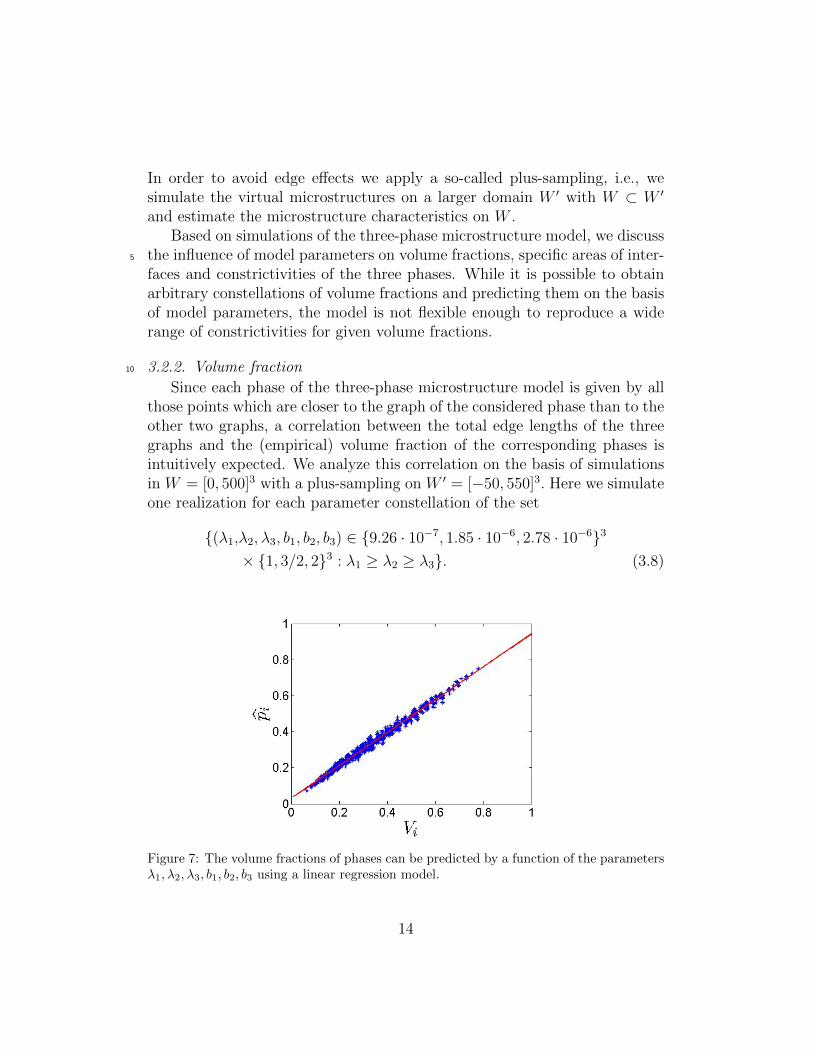
In order to avoid edge effects we apply a so-called plus-sampling, i.e., wesimulate the virtual microstructures on a larger domain W ′ with W ⊂ W ′

and estimate the microstructure characteristics on W .Based on simulations of the three-phase microstructure model, we discuss

the influence of model parameters on volume fractions, specific areas of inter-5

faces and constrictivities of the three phases. While it is possible to obtainarbitrary constellations of volume fractions and predicting them on the basisof model parameters, the model is not flexible enough to reproduce a widerange of constrictivities for given volume fractions.

3.2.2. Volume fraction10

Since each phase of the three-phase microstructure model is given by allthose points which are closer to the graph of the considered phase than to theother two graphs, a correlation between the total edge lengths of the threegraphs and the (empirical) volume fraction of the corresponding phases isintuitively expected. We analyze this correlation on the basis of simulationsin W = [0, 500]3 with a plus-sampling on W ′ = [−50, 550]3. Here we simulateone realization for each parameter constellation of the set

{(λ1,λ2, λ3, b1, b2, b3) ∈ {9.26 · 10−7, 1.85 · 10−6, 2.78 · 10−6}3

× {1, 3/2, 2}3 : λ1 ≥ λ2 ≥ λ3}. (3.8)

Figure 7: The volume fractions of phases can be predicted by a function of the parametersλ1, λ2, λ3, b1, b2, b3 using a linear regression model.

14

We describe the relationship between (empirical) volume fractions andthe values

Vi =eλi,bi

eλ1,b1 + eλ2,b2 + eλ3,b3(3.9)

by the following linear regression model

pi = 0.9132Vi + 0.0292 + ε1,i (3.10)

for each i ∈ {1, 2, 3}, where ε1,i is normally distributed with mean 0 andstandard deviation 0.013, i.e. ε1,i ∼ N(0, 0.0132). Besides the good visual fit,5

as shown in Figure 7, the coefficient of determination R2 = 0.99 indicatesa high predictability of the volume fractions by the total edge lengths andtherefore, in view of Equation (3.6), by the model parameters. In order tovalidate the obtained regression model, 100 further realizations have beensimulated where the parameters were randomly chosen. This means that all10

parameters are independently and uniformly distributed in certain intervals,to be more precise λi ∼ U(9.26 · 10−7, 2.78 · 10−6) and bi ∼ U([1, 2]) foreach i ∈ {1, 2, 3}. The errors pi − 0.9132Vi − 0.0292 obtained by simulationhave (empirical) mean and (empirical) standard deviation of 0.01 and 0.017,respectively, which shows that the linear regression model fits the relationship15

between volume fractions and expected total edge lengths very well.The derived relationship between expected total edge lengths and vol-

ume fractions allows us to reduce the vector of (free) model parameters(λ1, λ2, λ3, b1, b2, b3) under the condition that the volume fractions p1, p2 andp3 are fixed. Namely using Equations (3.6) and (3.10), for given volume20

fractions and given model parameters λ1, b1, b2, b3, we get the approximation

λi ≈ λ1

(pip1

)3/2(3bi − 1

3b1 − 1

)2

(3.11)

for each i ∈ {2, 3}. This approximation can be improved by solving Equa-tion (3.10) for λ2 and λ3.

3.2.3. Specific area of interfaces25

Besides the relationship derived in Section 3.2.2 between model param-eters and volume fractions of the three phases there is a strong correlationbetween volume fractions and specific areas of interfaces. Here an analogy tovery simple three-phase models, so-called independent tiling models can bedrawn.30

15

Figure 8: Relationship between the expressions (Ii,j + Ii,k)/(Ii,j + Ij,k) and (pi(pj +pk))/(pj(pi+pk)) estimated from simulated three-phase microstructures. The line throughthe origin with slope 1 is drawn in red.

Consider the following regular tilings of space: A square grid in 2D, ahexagonal grid in 2D, and a cubic grid in 3D. Then, the corresponding inde-pendent tiling model of such grids is defined in the following way: The originis located at random in one of the cells of the considered grid and each cell isindependently assigned to Ξi with probability pi for each i ∈ {1, 2, 3}, where5

p1, p2, p3 ≥ 0 and p1 + p2 + p3 = 1. For these three independent tiling modelsit is not difficult to show that the following relationship

Ii,j + Ii,kIi,j + Ij,k

=pi(pj + pk)

pj(pi + pk)(3.12)

holds. We denote the left-hand side by Si,j,k = (Ii,j + Ii,k)/(Ii,j + Ij,k) andthe right-hand side by Ri,j,k = (pi(pj + pk))/(pj(pi + pk)) for abbreviation.

Simulating 3D realizations with our microstructure model for the same10

parameter set as in Section 3.2.2, we can estimate Si,j,k and Ri,j,k. The cor-

responding estimators are denoted by Si,j,k = (Ii,j + Ii,k)/(Ii,j + Ij,k) and

Ri,j,k = (pi(pj + pk))/(pj(pi + pk)). Figure 8 shows that the developed mi-crostructure model behaves rather similar as the independent tiling modelwith respect to the specific areas of interfaces. The reason for this analogy15

might be the strong independence property between the three graphs. Wecome back to this analogy in Section 4.4.

16

3.2.4. Constrictivity

Figure 9: Relationship between constrictivity βi,W and pi estimated from simulated three-phase microstructures. The model introduced in Section 3.2.1 is not able to generateconstrictivities in a sufficiently wide range for a given volume fraction. The red line showsthe fit by linear regression between log pi and βi,W .

For the same realizations of our microstructure model that were used inSection 3.2.2 for the investigation of the relationship between model param-eters and volume fractions, the constrictivities β1,W , β2,W , β3,W with W =[0, 500]3 have been estimated. The results are visualized in Figure 9. One5

can observe that the model introduced in Section 3.2.1 is not flexible enoughwith respect to constrictivity since there is a strong correlation between vol-ume fraction and constrictivity of the same phase. This correlation can bemodeled by

βi,W = 0.35 log pi + 0.8 + ε2,i (3.13)

with ε2,i ∼ N(0, 0.0282). The coefficient of determination is 0.95.10

This absence of flexibility regarding constrictivity can be explained bythe fact that each phase is in some sense homogeneously located around thecorresponding graph. Homogeneity means here that there are no regions ofthe graph which tend to attract the corresponding phase more than oth-ers. Thus there are less bottlenecks in the phases than this is required for15

a systematic variation of volume fractions and constrictivities in virtual mi-crostructures. This problem will be solved by a generalization of the modelin Section 3.3. Furthermore, in the context of the generalized model, we will

17

describe the estimation of all model parameters in order to achieve a goodfit to experimental image data of three-phase microstructures in Section 4.

Nevertheless, we have created a simple parametric stochastic microstruc-ture model for three phase materials where it is possible to choose the param-eters in such a way that all phases are completely connected with probability5

1 and the volume fractions of phases can be predicted by the aid of modelparameters. Note that the model can be easily simulated without any kindof iterative procedure.

3.3. Generalization of the model

The generalized three-phase microstructure model is defined in the same10

way as the model presented in Section 3.2, but when we decide to which phasean arbitrary point x ∈ W belongs, we do not use the Euclidean distanceanymore. Instead, we use a parametric distance such that by variation of theparameter the corresponding phase is more or less accumulated around thevertices of the graph. The generalized model is formally defined as follows.15

Let γ1, γ2, γ3 ≥ 1 and let G1, G2, G3 be the beta-skeletons introduced inSection 3.2. The three phases are now defined by random sets Ξi, i = 1, 2, 3,such that

x ∈ Ξi iff d′γi(x,Gi) ≤ minj∈{1,2,3}

d′γj(x,Gj), (3.14)

whered′γi(x,Gi) = min{γid(x,Gi), d(x,Xi)}. (3.15)

Here d(x,Xi) = miny∈Xi|x − y| is the minimum Euclidean distance from x20

to the set of vertices Xi.The new distance measure d′γ fulfills d′γ(x,G) = 0 for each x located on the

edge set of the graph G and for each admissible γ. Thus in the generalizedmodel it is still valid that all three phases are completely connected withprobability 1 in case that 1 ≤ bi ≤ 2 for each i ∈ {1, 2, 3}. If γ = 1 it holds25

that d′γ(x,G) = d(x,G), i.e. d′γ(x,G) coincides with the Euclidean distancefrom x to G. With increasing γ the distance from x to the graph increases.However, this increase becomes smaller the closer x is to the nearest vertexof the graph G as shown in Figure 10.

Figure 11 shows the development of constrictivity in case that the param-30

eters λ1, λ2, λ3, b1, b2, b3 are fixed, where λ1 = λ2 = λ3 = 1.25 ·10−5, b1 = b2 =b3 = 1.5 and γ1 = γ2 = γ3 = γ where γ is varied between 1 and 10. Notethat in this case it holds that p1 = p2 = p3 = 1/3. One can observe that with

18

Figure 10: Contour lines of the distance to a given graph represented in blue with respectto d′γ for γ = 2 (left) and γ = 4 (right).

increasing γ, constrictivity decreases for γ ≥ 2. This is not surprising dueto the definition of d′γ wherein each phase is more accumulated around thevertices with increasing γ while the volume fraction does not change. Thisleads to the occurrence of bottlenecks and thus to decreasing constrictivities.The small increase of constrictivity for γ < 2 is due to a faster decrease of5

rmax than rmin for small γ.Finally, in a last step, the model is further generalized. The boundary

of the three phases is smoothed in order to have the possibility to decreasethe length of TPB. For this purpose we define a kind of Gaussian smoothingfor three-phase microstructures. At first we smooth the boundary between10

pores and the union of Ni and YSZ phases by a Gaussian smoothing. In asecond step the boundary between Ni and YSZ phases is also smoothed bya Gaussian smoothing.

We consider a function F on R3, which allocates a real number to eachvoxel according to the phase x belongs to. Furthermore, let θ > 0 and15

consider the function

ϕF (x) =

∫R3 F (y) · exp(− |x−y|

2

2θ2) dy∫

R3 exp(− |x−y|22θ2

) dy(3.16)

for each x ∈ R3 ∩ W . In particular, we choose the function F1 on R3 asF1(x) = 1 if x ∈ Ξ1 and F1(x) = 2 otherwise. Moreover, we define thefunction F2 on R3 by F2(x) = 3/2 if x ∈ Ξ1, F2(x) = 2 if x ∈ Ξ2 and F2(x) = 1otherwise. Then, the phases of the smoothed microstructure, denoted by20

19

Figure 11: Constrictivity βi over γ estimated for the three-phase microstructure modelwith parameters λ1 = λ2 = λ3 = 1.25 · 10−5, b1 = b2 = b3 = 1.5, γ1 = γ2 = γ3 = γ. Foreach parameter set, 9 realizations on W = [0, 500]3 are simulated.

Ξ′1,Ξ′2,Ξ

′3, are given by Ξ′1 = {x ∈ R3 : ϕF1(x) ≤ 1}, Ξ′2 = {x ∈ R3 :

ϕF1(x) ≥ 1, ϕF2(x) ≤ 3/2} and Ξ′3 = {x ∈ R3 : ϕF1(x) ≥ 1, ϕF2(x) ≥ 3/2}.For simulation purposes, the smoothing is applied on the discretized mi-

crostructure.Thus to compute ϕF1 and ϕF2 , we approximate the integrals inthe definition of ϕF by sums, i.e., ϕF is approximated by ϕF defined by5

ϕF (x) =

∑y∈V F (y) · exp(− |x−y|

2

2θ2)∑

y∈V exp(− |x−y|22θ2

), (3.17)

for each x ∈ V , where V denotes the set of all voxels in W .After the application of smoothing the complete connectivity of the three

phases can not be guaranteed in general. However, simulations show that forsmall values of the smoothing parameter θ the connectivity of the phases isstill very good, see Table 2 in Section 4.1.10

Note that the three-phase microstructure model originally introduced inSection 3.2.1 has been generalized such that the number of parameters isincreased from 6 to 10. By this generalization a better control over constric-tivity of the phases and over the length of TPB is achieved.

20

4. Model fitting and validation

4.1. Image data of Ni-YSZ anodes

Having defined the generalized three-phase microstructure model we showthat this model is able to describe complex 3D experimental image data repre-senting real Ni-YSZ anodes. We fit our model to the fine Ni-YSZ microstruc-5

ture in SOFC anodes before degradation which was recently described andanalyzed in [25]. The data obtained by FIB-tomography is visualized inFigure 12. The data represents a Ni-YSZ anode on a rectangular cuboidW = [0, 20µm]× [0, 25µm]× [0, 15µm] with a resolution of 30nm.

Figure 12: Left: 3D experimental image data of Ni-YSZ anodes. Pores are represented inblack, the YSZ phase in dark gray and the Ni phase in light gray. Center: Scaled imagedata. Right: Simulated microstructure with fitted parameters.

In experimental image data anisotropy effects with respect to chord-length10

distributions can be observed in Figure 13. For all three phases and for alllengths greater than 1 µm, the estimated distribution functions of chordlengths in z− direction is smaller than the distribution functions in x− andy− direction. This indicates that all three phases are elongated in z− direc-tion.15

Since the considered material is not expected to have such anisotropy,these effects in experimental image data are ascribed to FIB-imaging. Thuswe scale the image data in order to obtain an isotropic structure. Note that ascaling of the image data influences TPB since the scaling changes the voxelsize. However, different kinds of scaling have a different influence on TPB.20

In case that scaling is combined with a smoothing of the image the TPBdecreases.

21

Figure 13: Distribution functions of chord lengths with respect to the three main directionsestimated from experimental image data. The black (red, blue) curve represents thedistribution functions of chord lengths in x− (y−, z−) direction. From left to right:Distribution functions of chord lengths for pores, YSZ and Ni.

Figure 14: Nearest-neighbor interpolation in 2D. The original voxel grid is represented inblue, the transformed voxel grid in orange. The centers of voxels are represented by smalldisks in the corresponding colour.

For the purpose of scaling we use the so-called nearest-neighbor interpo-lation visualized in Figure 14. It turns out that a scale of the z−directionby 0.88 leads to the best result with respect to the accordance of distribu-tion functions of chord lengths in the three main directions. After scalingwe obtain a new voxel grid and we have to determine the phase of each of5

these new voxels. For this purpose, for each center c of a new voxel v weconsider the voxel w in the original grid the center of which is closest to c.Then, the voxel v belongs to the same phase as w. Figure 15 shows thatthe scaled image can be considered as isotropic with respect to chordlengthdistributions. The result of scaling is visualized in the center of Figure 12.10

Table 1 shows the microstructure characteristics described in Section 2 forexperimental image data before and after the scaling. The transport relevantcharacteristics are computed with respect to the transport directions in theNi-YSZ anode. It can be observed that the characteristics are hardly changed

22

Figure 15: Distribution functions of chord lengths in the three main directions estimatedfrom transformed image data. The black (red, blue) curve represents the distributionfunctions of chord lengths in x− (y−, z−) direction. From left to right: Distributionfunctions of chord lengths for pores, YSZ phase and Ni phase.

p1 p2 p3 τ1 τ2 τ3 β1 β2 β3 δ1Tomo. 0.26 0.42 0.32 1.28 1.11 1.18 0.30 0.41 0.29 0.0033

Tomo. scaled 0.25 0.42 0.33 1.26 1.10 1.17 0.31 0.42 0.33 0.0036Simulation 0.28 0.40 0.32 1.17 1.10 1.13 0.24 0.44 0.33 0.0035

Table 1: Comparison of microstructure characteristics for scaled tomography data, tomog-raphy data and simulated data. The different phases are numbered in the following way:1 - Pores, 2 - YSZ, 3 - Ni.

by the scaling.In experimental image data it can be seen that the three phases are almost

completely connected. As a measure for connectivity we compute the fractionci,x(ci,y, ci,z) of each phase i ∈ {1, 2, 3} that is connected in x − (y−, z−)direction. The results are given in Table 2. All values are close to one,5

which indicates a high connectivity. Thus it is appropriate to model thegiven experimental image data by a stochastic model that reproduces theseconnectivity properties.

c1,x c1,y c1,z c2,x c2,y c2,z c3,x c3,y c3,zTomo. 0.987 0.985 0.987 1.000 1.000 1.000 0.986 0.987 0.986

Tomo. scaled 0.988 0.985 0.987 0.999 0.999 0.999 0.986 0.987 0.986Simulation 1.000 1.000 1.000 0.997 0.997 0.997 1.000 1.000 1.000

Table 2: Comparison of connectivity for tomography data, scaled tomography data andsimulated data. For each i ∈ {1, 2, 3} the value ci,x denotes the fraction of the i-th phasethat is connected in x−direction. The definition of ci,y and ci,z is analogous. The differentphases are numbered in the following way: 1 - Pores, 2 - YSZ, 3 - Ni.

23

4.2. Fit of model parameters to experimental image data

Moreover, in Table 1 microstructure characteristics of experimental imagedata and the stochastic model are compared. Note that the parameters ofthe stochastic model are fitted to the volume fractions, length of TPB andto geodesic tortuosities as well as constrictivities of Ni and YSZ, i.e., we5

minimize the following cost function of relative errors between microstructurecharacteristics of simulated and scaled image data:

33∑i=2

|pi,sim − pi|pi

+ 23∑i=2

|βi,sim − βi|βi

+3∑i=2

|τi,sim − τi|τi

+|δ1,sim − δ1|

δ1

. (4.1)

For this purpose we use the Nelder-Mead method introduced in [23]. Thismethod, also called downhill-simplex method is a direct search method, i.e.,it is used for non-linear optimization without using derivatives of the func-10

tion that has to be minimized. Although there are not many results aboutconvergence of this method it is successfully used in many applications. Thisis adequate here since we do not need to find the best, but a sufficiently goodparameter constellation, which shows that the model is able to generate real-istic microstructures. For more information about the Nelder-Mead method15

the reader is referred to [7].

Parameters Fitted valuesλ1 0.87µm−3

λ2 1.18µm−3

λ3 0.95µm−3

b1 2.11b2 1.97b3 1.94γ1 4.47γ2 4.31γ3 4.12θ 0.69

Table 3: Parameters fitted by the Nelder-Mead method.

The microstructure characteristics for a certain parameter set are esti-mated on the basis of simulations on W = [0, 15µm]3 with voxel size 30nm.By the Nelder-Mead method the optimal parameter set given in Table 3 isobtained. It leads to a very good fit with respect to the microstructure char-20

acteristics that are considered in the cost function, i.e. p2, p3, β2, β3, τ2, τ3, δ1.

24

Note that the remaining characteristics mean geodesic tortuosity τ1 and con-strictivity β1 of pores are not taken into account in the cost function. How-ever, the microstructure characteristics of the simulated microstructures arequite similar to the ones of experimental data. Moreover, note that the fittingprocedure leads to b1 = 2.11 > 2. Thus the complete connectivity of Ξ1 is not5

theoretically guaranteed. However, computation of connectivity properties,see Table 2 in Section 4.1, shows that this parameter constellation does alsolead to almost complete connectivity of Ξ1. In the considered realizations thephase Ξ1 is even completely connected. Note that the values in Table 2 con-cerning Ni and YSZ phases that are smaller than 1 are caused by edge effects.10

4.3. Model validation

To validate the model introduced in Section 3.3 the ratio between ef-fective and intrinsic conductivities denoted by σeff and σ0, respectively, ofNi and YSZ phases are computed using the FE-method and the length of15

TPB is computed by the estimator δ2 described in Section 2.4. Note thatFE-simulations have been performed by the software GeoDict [11].

σeff/σ0 for YSZ phase σeff/σ0 for Ni phase δ2Tomo. 0.154 0.074 2.34µm−2

Tomo. scaled 0.162 0.078 2.53µm−2

Simulation 0.152 0.087 2.77µm−2

Table 4: Comparison of effective conductivities for Ni and YSZ phases and of the estimatedTPB for tomography data, scaled tomography data and simulated data.

The results are given in Table 4. Note that the three characteristics con-sidered in this table are not used for model fitting. Nevertheless, we havea good accordance between simulated effective conductivities and lengths of20

TPB. Especially the effective conductivities of the YSZ phase for experimen-tal and simulated image data are quite close to each other. The model isthus able to capture these characteristics of Ni-YSZ anodes which are mostimportant for the performance of the cell.

4.4. Specific area at phase boundaries - limitations of the model25

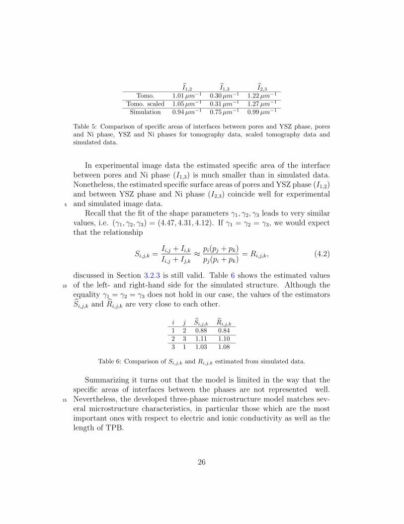
Table 5 shows limitations of the stochastic microstructure model intro-duced in Section 3.3 since the model is not flexible enough with respect tothe specific area at the phase boundaries.

25

I1,2 I1,3 I2,3Tomo. 1.01µm−1 0.30µm−1 1.22µm−1

Tomo. scaled 1.05µm−1 0.31µm−1 1.27µm−1

Simulation 0.94µm−1 0.75µm−1 0.99µm−1

Table 5: Comparison of specific areas of interfaces between pores and YSZ phase, poresand Ni phase, YSZ and Ni phases for tomography data, scaled tomography data andsimulated data.

In experimental image data the estimated specific area of the interfacebetween pores and Ni phase (I1,3) is much smaller than in simulated data.Nonetheless, the estimated specific surface areas of pores and YSZ phase (I1,2)and between YSZ phase and Ni phase (I2,3) coincide well for experimentaland simulated image data.5

Recall that the fit of the shape parameters γ1, γ2, γ3 leads to very similarvalues, i.e. (γ1, γ2, γ3) = (4.47, 4.31, 4.12). If γ1 = γ2 = γ3, we would expectthat the relationship

Si,j,k =Ii,j + Ii,kIi,j + Ij,k

≈ pi(pj + pk)

pj(pi + pk)= Ri,j,k, (4.2)

discussed in Section 3.2.3 is still valid. Table 6 shows the estimated valuesof the left- and right-hand side for the simulated structure. Although the10

equality γ1 = γ2 = γ3 does not hold in our case, the values of the estimatorsSi,j,k and Ri,j,k are very close to each other.

i j Si,j,k Ri,j,k1 2 0.88 0.842 3 1.11 1.103 1 1.03 1.08

Table 6: Comparison of Si,j,k and Ri,j,k estimated from simulated data.

Summarizing it turns out that the model is limited in the way that thespecific areas of interfaces between the phases are not represented well.Nevertheless, the developed three-phase microstructure model matches sev-15

eral microstructure characteristics, in particular those which are the mostimportant ones with respect to electric and ionic conductivity as well as thelength of TPB.

26

5. Conclusion and outlook

In the present paper a parametric stochastic microstructure model for de-scription and simulation of three-phase Ni-YSZ anodes was developed usingmethods from stochastic geometry. The model is constructed such that forvarious parameter sets all three phases are completely connected with prob-5

ability 1. Furthermore, we were able to fit the parameters of our model toexperimental 3D image data.

We started with a model consisting of 6 parameters, where three beta-skeletons on homogeneous Poisson point processes were modeled. Each graphbuilds the backbone of one of the three phases. Each phase is then given by10

these points which are closer (with respect to the Euclidean distance) to thecorresponding graph than to the other two graphs. For this model a rela-tionship between the expected total edge length of the three beta-skeletonsand the volume fraction of the phases was established by a simulation study.Thus it is possible to describe three-phase microstructures with completely15

connected phases and to adjust the volume fraction by the model parame-ters. For fitting the model to experimental image data a generalization ofthe model was necessary. In order to determine to which phase a certainpoint belongs, we consider a (modified) parametric distance to the threegraphs and the boundary of the three phases is smoothed according to an20

additional parameter. Finally we arrive at a 10-parametric model, which isfitted successfully to experimental image data with respect to the followingtransport relevant microstructure characteristics: Volume fractions, meangeodesic tortuosities, constrictivities of the three phases and the length ofTPB. Note that the developed model can be easily simulated in short time,25

which is also caused by the fact that the simulation does not involve anyiterative procedure.

Using the FE-method the effective conductivities in the Ni and YSZphases of simulated and experimental data have been computed. It turnedout that experimental and simulated data are in good accordance to each30

other. This shows that the realizations of the model can be considered as real-istic Ni-YSZ microstructures. Moreover, we were able to reduce the complexinformation of the 3D images to 10 real-valued parameters, which containthe decisive information about conductivity in the Ni and YSZ phases.

In further work we will vary the parameters of the stochastic model in35

order to obtain virtual, but realistic Ni-YSZ microstructures with differenttransport relevant microstructure characteristics. Using the FE-method and

27

simulating the anode reaction mechanism on these virtual structures we cangenerate a large database in order to efficiently investigate the quantitativerelationship between microstructure characteristics and the anode perfor-mance. The results of such an investigation can be validated by a few ex-perimental measurements of real anodes. Therefore, this approach, based on5

virtual materials design performed by stochastic modeling, can be used forreliable microstructure optimization with a reduced experimental effort.

Note that the presented approach can be modified in different ways formodeling three-phase microstructures. In particular one could think of amodification towards Ni-YSZ microstructures with a bimodal pore size dis-10

tribution, which was observed for the data presented in [31]. For this purpose,it might be possible to use other point process models for the vertices of thegraph and to incorporate dependencies between the three point processes, in-stead of the model generalization considered in Sectio 3.3. Moreover, anotherclass of connected geometric graphs can be chosen instead of the beta-skeleton15

for modeling the edges. So the presented approach opens new possiblities inthe modeling of three-phase microstructures, which can be used in future foroptimization of electrode microstructures by virtual materials design.

Acknowledgments

The authors like to thank Ole Stenzel for helpful discussions. The re-20

search presented in this paper has received funding from the Swiss NationalScience Foundation (SNSF, Grant Nr. 407040 154047), from the GermanAcademic Exchange Service (DAAD) as well as from the Czech Ministeryof Education (Project 7AMB14DE006). All financial supports are gratefullyacknowledged.25

Appendix A.

Proof of Proposition 1. At first, note that Ab(x, y) is the union of two equallysized hyperspherical caps. The height of these hyperspherical caps is givenby h = |x− y|/2 and the radius of the corresponding sphere is

r = |(b/2)x+ (1− b/2)y − y| = b/2 · |x− y|. (A.1)

Due to results from [19] it is not difficult to see that30

νd(Ab(x, y)) =2

Γ(d+1

2

)π d−12

(b

2|x− y|

)d ∫ arccos(1− 1b)

0

sind(t) dt. (A.2)

28

Now we continue with the calculation of eλ,b where we use the notation

α = λνd(Ab(x, y))/|x− y|d. (A.3)

By the Slivnyak-Mecke theorem, see Theorem 3.3 in [21], we obtain

eλ,b =λ2

2

∫Rd

∫Rd

P (X ∩ Ab(x, y) = ∅)H1([x, y] ∩ [0, 1]d) dxdy,

=λ2

2

∫Rd

∫Rd

∫ 1

0

1(µx+ (1− µ)y ∈ [0, 1]d)|x− y|

exp(−α|x− y|d) dµdxdy. (A.4)

By the substitution x = z + y we get

eλ,b =λ2

2

∫Rd

∫Rd

∫ 1

0

1(µz + y ∈ [0, 1]d)|z| exp(−α|z|d) dµdzdy

Fubini=

λ2

2

∫Rd

∫ 1

0

∫Rd

1(y ∈ [0, 1]d − µz)|z| exp(−α|z|d) dydµdz

=λ2

2

∫Rd

|z| exp(−α|z|d) dz = dκdλ2

∫ ∞0

td exp(−αtd) dt, (A.5)

where last line of (A.5) is obtained by substitution of Euclidean coordinatesby spherical coordinates. Here κd = πd/2/Γ(d/2 + 1) denotes the volume ofthe d-dimensional ball. Integration by parts leads to the claim

eλ,b =dκdλ

2

2

((−tdα

exp(−αtd))∣∣∣∣∞

0

+

∫ ∞0

1

dαexp(−αtd) dt

)=κdλ

2

2α

∫ ∞0

exp(−αtd) dt =κdλ

2

2dα1+ 1d

Γ

(1

d

)=

2d−1+ 1dλ1− 1

dπ12d

bd+1d(∫ arccos(1− 1

b)

0sind(t) dt

)1+ 1d

(Γ(d+1

2

))1+ 1d Γ(

1d

)Γ(d2

+ 1) . (A.6)

References

[1] D. J. Aldous and J. Shun. Connected spatial networks over randompoints and a route-length statistic. Statistical Science, 25(3):275–288,5

2010.

29

[2] A. Bertei, C. C. Chueh, J. G. Pharoah, and C. Nicolella. Modifiedcollective rearrangement sphere-assembly algorithm for random packingsof nonspherical particles: Towards engineering applications. PowderTechnology, 253:311–324, 2014.

[3] Q. Cai, C. S. Adjiman, and N. P. Brandon. Modelling the 3D microstruc-5

ture and performance of solid oxide fuel cell electrodes: Computationalparameters. Electrochimica Acta, 56(16):5804–5814, 2011.

[4] S. N. Chiu, D. Stoyan, W. S. Kendall, and J. Mecke. Stochastic Geometryand its Applications. J. Wiley & Sons, Chichester, 3rd edition, 2013.

[5] H. W. Choi, A. Berson, J. G. Pharoah, and S. B. Beale. Effective10

transport properties of the porous electrodes in solid oxide fuel cells.Proceedings of the Institution of Mechanical Engineers, Part A: Journalof Power and Energy, 225(2):183–197, 2011.

[6] M. B. Clennell. Tortuosity: a guide through the maze. Geological Soci-ety, London, Special Publications, 122(1):299–344, 1997.15

[7] A. R. Conn, K. Scheinberg, and L. N. Vicente. Introduction toDerivative-free Optimization. SIAM, Society for Industrial and AppliedMathematics, Philadelphia, PA, 2009.

[8] P. Costamagna, P. Costa, and V. Antonucci. Micro-modelling of solidoxide fuel cell electrodes. Electrochimica Acta, 43(3):375–394, 1998.20

[9] P. F. Felzenszwalb and D. P. Huttenlocher. Distance transforms of sam-pled functions. Theory of Computing, 8:415–428, 2009.

[10] G. Gaiselmann, M. Neumann, O. M. Pecho, T. Hocker, V. Schmidt,and L. Holzer. Quantitative relationships between microstructure andeffective transport properties based on virtual materials testing. AIChE25

Journal, 60(6):1983–1999, 2014.

[11] GeoDict - open source software. www.geodict.com, 2014.

[12] J. Golbert, C. S. Adjiman, and N. P. Brandon. Microstructural model-ing of solid oxide fuel cell anodes. Industrial & Engineering ChemistryResearch, 47(20):7693–7699, 2008.30

30

[13] C. Hirsch, D. Neuhauser, and V. Schmidt. Connectivity of random geo-metric graphs related to minimal spanning forests. Advances in AppliedProbability, 45(1):20–36, 2013.

[14] L. Holzer, B. Iwanschitz, T. Hocker, L. Keller, O. M. Pecho, G. Sartoris,P. Gasser, and B. Muench. Redox cycling of Ni–YSZ anodes for solid5

oxide fuel cells: Influence of tortuosity, constriction and percolation fac-tors on the effective transport properties. Journal of Power Sources,242:179–194, 2013.

[15] L. Holzer, B. Munch, B. Iwanschitz, M. Cantoni, T. Hocker, andT. Graule. Quantitative relationships between composition, particle size,10

triple phase boundary length and surface area in nickel-cermet anodesfor solid oxide fuel cells. Journal of Power Sources, 196(17):7076–7089,2011.

[16] B. Kenney, M. Valdmanis, C. Baker, J. G. Pharoah, and K. Karan.Computation of tpb length, surface area and pore size from numerical15

reconstruction of composite solid oxide fuel cell electrodes. Journal ofPower Sources, 189(2):1051–1059, 2009.

[17] J. F. C. Kingman. Poisson Processes, volume 3. Oxford UniversityPress, Oxford, 1992.

[18] D. R. Kirkpatrick and J. D. Radke. A framework for computational20

geometry. In G. T. Toussaint, editor, Computational Geometry, pages217–248. North-Holland, Amsterdam, 1985.

[19] S. Li. Concise formulas for the area and volume of a hyperspherical cap.Asian Journal of Mathematics and Statistics, 4(1):66–70, 2011.

[20] C. Metcalfe, O. Kesler, T. Rivard, F. Gitzhofer, and N. Abatzoglou.25

Connected three-phase boundary length evaluation in modeled sinteredcomposite solid oxide fuel cell electrodes. Journal of the ElectrochemicalSociety, 157(9):B1326–B1335, 2010.

[21] J. MAyller and R. P. Waagepetersen. Statistical Inference and Simula-tion for Spatial Point Processes. Chapman & Hall/CRC, Boca Raton,30

2004.

31

[22] B. Munch and L. Holzer. Contradicting geometrical concepts in poresize analysis attained with electron microscopy and mercury intrusion.Journal of the American Ceramic Society, 91(12):4059–4067, 2008.

[23] J. A. Nelder and R. Mead. A simplex method for function minimization.The Computer Journal, 7:308–313, 1965.5

[24] J. Ohser and K. Schladitz. 3D Images of Materials Structures: Process-ing and Analysis. J. Wiley & Sons, Weinheim, 2009.

[25] O. M. Pecho, O. Stenzel, P. Gasser, M. Neumann, V. Schmidt,T. Hocker, R. J. Flatt, and L. Holzer. 3D microstructure effects inNi-YSZ anodes: Prediction of effective transport properties and opti-10

mization of redox-stability. Materials, 8(9):5554–5585, 2015.

[26] J. G. Pharoah, L. Handl, and V. Schmidt. The effect of electrode mor-phology on solid oxide fuel cell performance. ECS Transactions, 68:2037–2045, 2015.

[27] B. S. Prakash, S. S. Kumar, and S. T. Aruna. Properties and develop-15

ment of Ni/YSZ as an anode material in solid oxide fuel cell: A review.Renewable and Sustainable Energy Reviews, 36:149–179, 2014.

[28] N. Shikazono, D. Kanno, K. Matsuzaki, H. Teshima, S. Sumino, andN. Kasagi. Numerical assessment of SOFC anode polarization based onthree-dimensional model microstructure reconstructed from FIB-SEM20

images. Journal of the Electrochemical Society, 157(5):B665–B672, 2010.

[29] O. Stenzel, O. M. Pecho, M. Neumann, V. Schmidt, and L. Holzer.Predicting effective conductivities based on geometric microstructurecharacteristics. AIChE Journal, in print, 2016.

[30] K. Thulasiraman and M. N. S. Swamy. Graphs: Theory and Algorithms.25

J. Wiley & Sons, New York, 1992.

[31] J. Villanova, J. Laurencin, P. Cloetens, P. Bleuet, G. Delette, H. Suho-nen, and F. Usseglio-Viretta. 3D phase mapping of solid oxide fuel cellYSZ/Ni cermet at the nanoscale by holographic X-ray nanotomography.Journal of Power Sources, 243:841–849, 2013.30

32

[32] J. R. Wilson, W. Kobsiriphat, R. Mendoza, H.-Y. Chen, J. M. Hiller,D. J. Miller, K. Thornton, P. W. Voorhees, S. B. Adler, and S. A. Bar-nett. Three-dimensional reconstruction of a solid-oxide fuel-cell anode.Nature Materials, 5(7):541–544, 2006.

33