279
STOCHASTIC DYNAMIC RESPONSE OF A TENSION LEG PLATFORM OYEJOBI DAMILOLA OYEWUMI FACULTY OF ENGINEERING UNIVERSITY OF MALAYA KUALA LUMPUR 2017
STOCHASTIC DYNAMIC RESPONSE OF A TENSION LEG PLATFORM
OYEJOBI DAMILOLA OYEWUMI
FACULTY OF ENGINEERING UNIVERSITY OF MALAYA
KUALA LUMPUR
2017
STOCHASTIC DYNAMIC RESPONSE OF A TENSION LEG
PLATFORM
OYEJOBI DAMILOLA OYEWUMI
THESIS SUBMITTED IN FULFILMENT
OF THE REQUIREMENTS
FOR THE DEGREE OF DOCTOR OF PHILOSOPHY
FACULTY OF ENGINEERING
UNIVERSITY OF MALAYA
KUALA LUMPUR
2017
ii
ORIGINAL LITERARY WORK DECLARATION
Name of Candidate: OYEJOBI DAMILOLA OYEWUMI I.C/Passport NO: A04768367
Registration/ Matric No: KHA130140
Name of Degree: Doctor of Philosophy
Title of Thesis: Stochastic Dynamic Response of A Tension Leg Platform
Field of Study: Structural Engineering
I do solemnly and sincerely declare that:
(1) I am the sole author/ writer of this work; (2) This work is original; (3) Any use of any work in which copyright exists was done by way of fair dealing and
for permitted purposes and any excerpt or extract from, or reference to or reproduction of any copyright work has been disclosed expressly and sufficiently and the title of the work and its authorship have been acknowledged in this work;
(4) I do not have any actual knowledge nor do ought I reasonably to know that the making of this work constitutes an infringement of any copyright work;
(5) I hereby assign that all and every rights in the copyright to this work to the University of Malaya (UM), who henceforth shall be owner of the copyright of this work and that any reproduction or any use any form or by any means whatsoever is prohibited without the written consent of UM having been first had and obtained.
(6) I am fully aware that if in the course of making this work I have infringed any copy right whether intentionally or otherwise, I may be subject to legal action or any other action as may be determined by UM.
Candidate’s Signature Date
Subscribed and solemnly declared before,
Witness’s Signature Date Name: Designation

iii
ABSTRACT
A systematic formulation program for the computation of stochastic dynamic
response of a tension leg platform (TLP) was developed and solved for the uncoupled TLP.
The effect of tendon dynamics was incorporated into a coupled TLP and was discretized
using the finite element method. The platform was idealized as a rigid body and the
matrices of equation of motions were formulated and solved by numerical time integration.
The TLP response was characterized for regular, unidirectional and directional random
waves, as well as for current and wind forces. The ocean waves were simulated using the
small amplitude wave theory for regular wave and the Pierson Moskowitz wave spectrum
for unidirectional and directional ocean waves. The hydrodynamic forces on the TLP were
calculated by modified Morison equation while the wind-drift current on the TLP was
modelled with linear profile model. The aerodynamic loadings were computed by the
logarithmic wind speed profile for the mean wind speed and the Simiu- Leigh and
American Petroleum Institute (API) spectra were used for fluctuating wind component in
uncoupled and coupled TLP models respectively. The associated nonlinearity and
response-dependent nature of the TLP made the computation of equation of motions time
consuming. The results of the TLP responses were reported in time history, power
spectrum and statistical values. For regular wave characterization, the results revealed that
the platform amplified at the wave frequency only. In contrast with regular wave
modelling, the platform amplification in all degrees of freedom occurred predominantly at
the surge natural degree of freedom as well as at the wave frequency for unidirectional and
directional random waves. Current and wind drag forces caused steady offset displacements
in all degrees of freedoms. The motion and tendon tension responses in coupled TLP were
lower in magnitude compared to the uncoupled TLP except for surge response. The

iv
behaviour of TLP in parametric studies of varying wave heights, wave periods, different
sea states, loss of tendon from a group of tendon legs were analysed and reported for the
purpose of decision making.
This work avoided solving separate equations of motions for the platform model
and the tendon leg system but simultaneously coupled it together. This was accomplished
by coding the mathematical derivations in a high-level programming language and
commercial finite element tool. The finite element tool was not originally designed for the
solution of offshore platforms but was adapted for model discretization and the application
of hydrodynamic and aerodynamic loadings on the platform. The result of this research was
that offshore problem with high level complexities was solved using the knowledge of
Civil Engineering.

v
ABSTRAK
Satu program penggubalan sistematik untuk pengiraan sambutan dinamik
stokastik platform ketegangan kaki (PKK) telah dibangunkan dan diselesaikan untuk PKK
terlerai. Kesan dinamik tendon telah digabungkan ke dalam PKK terganding dan di
terdiskret menggunakan kaedah unsur terhingga. Platform ini telah diunggulkan sebagai
badan tegar dan matriks persamaan gerakan telah dirangka dan diselesaikan dengan
integrasi masa berangka. Sambutan PKK dicirikan untuk gelombang rawak biasa, searah
dan berarah, dan juga kuasa arus dan angin. Ombak lautan telah di simulasi menggunakan
teori gelombang amplitud kecil untuk gelombang biasa dan gelombang spektrum Pierson
Moskowitz bagi ombak lautan searah dan berarah. Kuasa hidrodinamik ke atas PKK telah
dikira dengan persamaan Morison yang diubahsuai, sementara arus aliran angin ke atas
PKK telah dimodelkan dengan model profil linear. Bebanan aerodinamik telah dikira
dengan profil kelajuan angin logaritma untuk kelajuan min angin dan Simiu-Leigh serta
spektrum API (Institut Petroleum Amerika) masing-masing digunakan untuk komponen
turun naik angin dalam model PKK terlerai dan terganding. Sifat PKK berkaitan
ketaklelurusan dan yang bersandarkan tindakbalas menjadikan pengiraan persamaan
pergerakan satu proses yang memakan masa. Hasil tindakbalas PKK dilaporkan dalam
sejarah masa, spektrum kuasa dan nilai statistik. Untuk pencirian gelombang biasa, hasil
dapatan menunjukkan bahawa platform dikuatkan pada frekuensi gelombang sahaja.
Berbeza dengan model gelombang biasa, penguatan platform bagi semua darjah kebebasan
berlaku lebih kerap pada darjah kebebasan semulajadi pusuan serta pada frekuensi
gelombang bagi gelombang rawak searah dan berarah. Kuasa seretan arus dan angin
menyebabkan pengubahan pengimbangan yang stabil dalam semua darjah kebebasan.
Tindakbalas pergerakan dan ketegangan tendon bagi PKK terganding adalah pada
magnitud yang lebih rendah berbanding dengan PKK terlerai kecuali dalam tindakbalas

vi
lonjakan. Kelakuan PKK dalam kajian parametrik ketinggian ombak berbeza-beza, tempoh
gelombang, keadaan laut yang berbeza, kehilangan tendon daripada sekumpulan kaki
tendon dianalisis dan dilaporkan untuk proses membuat keputusan.
Kajian ini telah mengelak dari menyelesaikan persamaan pergerakan berasingan
bagi model platform dan sistem tendon kaki tetapi telah mengandingkannya bersama secara
serentak. Ini telah dicapai dengan pengekodan pemerolehan matematik dalam bahasa
pengaturan komputer peringkat tinggi dan alat unsur terhingga komersial. Alat unsur
terhingga tidak pada asalnya direka bagi penyelesaian platform luar pesisir pantai tetapi
telah disesuaikan untuk pendiskretan model dan penggunaan bebanan hidrodinamik dan
aerodinamik keatas platform. Hasil kajian ini adalah bahawa masalah luar pesisir pantai
dengan kerumitan peringkat tinggi telah diselesaikan dengan menggunakan pengetahuan
Kejuruteraan Awam.

vii
ACKNOWLEDGEMENTS
Giving thanks to the LORD, the maker of heaven and earth and everything within universe
including me for he is good and his mercies endure forever.
It is my pleasure to extend my unreserved gratitude and sincere appreciation to my
academic professors in person of Dr. Mohammed Jameel and Associate Prof. Dr. Nor
Hafizah Binti Ramli @ Sulong of Department of Civil Engineering, University of Malaya
for their contribution in making this research a huge success.
I would like to thank Dr Lanre, Dr Dupe and Dr Taofeeq, it is very difficult to express my
gratitude in words for your respective roles. I am indebted to my amiable family, Beatrice,
Damilola and Damilare Oyejobi for your understanding and cooperation. I equally thank
my parents and siblings you have proved to me in several ways that blood is thicker than
water. To my late big cousin Bukola Ajayi, even in your death, you live every day in my
heart, love you and love your family.
Personal relationship with Damilola, Elizabeth, Hussein and Haider made a huge difference
to the success of this program. Thanks to my FORTRAN coach and thesis editor in persons
of Mr. Elliot Chandler and Dr (Mrs) Jawakhir Mior Jaafar that painfully went through my
FORTRAN codes and thesis respectively, you are very inspiring.
This acknowledgment would be incomplete if University of Malaya is not appreciated for
their financial supports from the University grants numbers RP004E-13AET and PB225-
2014B. To my spiritual fathers, Pastor (Dr) Gideon Iselewa and Bishop (Dr) Charles
Popson, thank you for your enthusiasm in my progress and unwavering belief in me during
the programme. It is very difficult to continue mentioning names, friends and well-wishers,
specifically, reader of this thesis, I thank you all.
To God immortal, invisible and eternal, be all the glory and bless this work in my hands,
Amen.

viii
TABLE OF CONTENTS
ORIGINAL LITERARY WORK DECLARATION ............................................................. ii
ABSTRACT .......................................................................................................................... iii
ABSTRAK ............................................................................................................................. v
ACKNOWLEDGEMENTS ................................................................................................. vii
TABLE OF CONTENTS .................................................................................................... viii
LIST OF FIGURES ............................................................................................................. xv
LIST OF TABLES ............................................................................................................... xx
LIST OF SYMBOLS AND ABBREVIATIONS .............................................................. xxii
LIST OF APPENDICES .................................................................................................. xxvii
CHAPTER 1: INTRODUCTION ....................................................................................... 1
1.1 Background .................................................................................................................. 1
1.2 Present State of the Problem ........................................................................................ 5
1.3 Aim and Objectives of the Study ................................................................................. 7
1.4 Scope of the Research .................................................................................................. 7
1.5 Structure of the Thesis .................................................................................................. 9
CHAPTER 2: LITERATURE REVIEW ......................................................................... 10
2.1 Introduction ................................................................................................................ 10
2.2 Description of Offshore Structures ............................................................................ 10
2.2.1 Fixed Offshore Structures ................................................................................. 10

ix
2.2.1.1 Jacket/Steel Template Structures ........................................................... 11
2.2.1.2 Gravity Base Structures ......................................................................... 12
2.2.1.3 Jack-up Structure ................................................................................... 13
2.2.2 Compliant Structures .......................................................................................... 14
2.2.2.1 Articulated Platforms ............................................................................. 15
2.2.2.2 Compliant Tower ................................................................................... 15
2.2.2.3 Guyed Tower ......................................................................................... 16
2.2.3 Floating Structures ............................................................................................... 17
2.2.3.1 Floating Production System ..................................................................... 18
2.2.3.2 Floating Production, Storage and Offloading System ............................. 18
2.2.3.3 Tension Leg Platform (TLP) ................................................................... 19
2.2.3.3 (a) Conventional TLP .................................................................. 19
2.2.3.3. (b) Extended TLP ........................................................................ 20
2.2.3.3 (c) SeaStar TLP ............................................................................ 20
2.2.3.3 (d) Mini-TLP ................................................................................. 21
2.3 Advantages of Tension Leg Platform ......................................................................... 25
2.4 Environmental Forces on Tension Leg Platform ....................................................... 26
2.4.1 Wave Forces ...................................................................................................... 26
2.4.2 Wind Forces ....................................................................................................... 26
2.4.3 Current Forces ................................................................................................... 27
2.4.4 Earthquakes........................................................................................................ 27

x
2.5 Wave Theory .............................................................................................................. 28
2.5.1 Linear Wave Theory ......................................................................................... 28
2.5.2 Stokes Wave Theory ......................................................................................... 28
2.5.3 Stream Function Theory ................................................................................... 29
2.5.4 Numerical Theory ............................................................................................. 29
2.6 Dynamic Analysis of Tension Leg Platform .............................................................. 29
2.6.1 Time and Frequency Domain Analyses ............................................................ 30
2.7. Analysis of Coupled and Uncoupled of TLP Models ............................................... 32
2.8 Finite Element Modelling of TLP .............................................................................. 35
2.9 Different Analysis Method and Load Combinations ................................................. 36
2.10 TLP-Tendon-Riser system ....................................................................................... 42
2.11 Summary of Previous works .................................................................................... 45
CHAPTER 3: METHODOLOGY .................................................................................... 46
3.0 Introduction ................................................................................................................ 46
3.1 TLP Structural Idealization and Assumptions ........................................................... 47
3.2 Derivation of Equations of Motion for TLP Platform ................................................ 50
3.2.1 Mass Matrix ....................................................................................................... 51
3.2.2 Damping Matrix................................................................................................. 52
3.2.3 Stiffness Matrix ................................................................................................. 54
3.2.3.1 Surge Motion .......................................................................................... 55
3.2.3.2 Sway Motion ............................................................................................ 57
xi
3.2.3.3 Heave Motion ............................................................................................ 59
3.2.3.4 Roll Motion ................................................................................................ 60
3.2.3.5 Pitch Motion .............................................................................................. 61
3.2.3.6 Yaw Motion ............................................................................................... 63
3.3 Simulation of Sea Waves and Water Particle Kinematics ......................................... 65
3.3.1 Regular Sea Waves ........................................................................................... 65
3.3.2 Random Sea Waves .......................................................................................... 67
3.3.2.1 Unidirectional and Directional Sea Waves ........................................... 67
3.4 Modified Morison Wave Force .................................................................................. 71
3.4.1 Simulation of Wave Force on Column and Pontoon ........................................ 72
3.4.2 Total Wave and Current Induced Forces .......................................................... 75
3.4.3 Current Force .................................................................................................... 76
3.4.4 Wind Forces ...................................................................................................... 76
3.4.4.1 Mean Wind Speed................................................................................. 77
3.4.4.2 Fluctuating Wind Velocity ................................................................... 78
3.5 Assembly and Solution of Equation of Motion for UNAP-TLP-2016 ...................... 79
3.6 Simulation of CNAP-TLP-2016 in Abaqus Software ................................................ 82
3.6.1 TLP Hull ............................................................................................................ 84
3.6.2 TLP Tendons ..................................................................................................... 86
3.6.3 Connector Elements ........................................................................................... 89
3.6.4 Numerical Solution for CNAP-TLP-2016 ......................................................... 89
xii
3.7 Summary .................................................................................................................... 91
CHAPTER 4: RESULTS AND DISCUSSION ............................................................... 92
4.1 Introduction ................................................................................................................ 92
4.2 Validation of UNAP-TLP-2016 with Published Result ............................................. 92
4.2.1 Comparison of UNAP-TLP-2016 Model Result for Regular Wave ................ 94
4.2.2 Validation of UNAP-TLP-2016 Model Result for Random Waves ............... 100
4.3 Numerical Study ....................................................................................................... 109
4.3.1 Comparison of Natural Periods of Oscillation of the ISSC TLP .................... 110
4.3.2 Response of an Uncoupled TLP in Regular and Random Waves .................. 111
4.3.3 Effect of Current Force on an Uncoupled TLP in Regular and Random Waves
.................................................................................................................................... 123
4.3.4 Effect of Wind Force on an Uncoupled TLP in Regular and Random Waves 129
4.4 Effect of the Sea States on TLP Motions ................................................................. 136
4.4.1 Effect of Current Velocity on the Sea States ................................................... 138
4.4.2 Effect of Wind Velocity on Sea States ............................................................ 139
4.4.3 Effect of Current and Wind Velocities on Sea States ...................................... 140
4.4.4 Effect of One Tendon Missing in Random Waves and Current Forces .......... 141
4.5 Verification of Coupled TLP Model ........................................................................ 143
4.5.1 Results of Static and Vibration Analysis ........................................................ 144
4.5.2 Verification of CNAP-TLP Model Motion with Published Results .............. 150

xiii
4.5.3 Validation of Massless Abaqus-TLP Model with UNAP-TLP Model ............. 155
4.6 Effect of Wave, Current and Wind Loads on the Response of CNAP-TLP Model . 161
4.6.1 Surge Time History.......................................................................................... 161
4.6.2 Heave Time History .......................................................................................... 164
4.6.3 Pitch Time History ............................................................................................ 166
4.6.4 Tendon Tension Time History .......................................................................... 168
4.7 Effect of Tendon Dynamics on TLP Response ........................................................ 171
4.8 TLP Response in Constant Wave Height and Varying Wave Period ...................... 173
4.8.1 Surge Response ............................................................................................... 174
4.8.2 Heave Response .............................................................................................. 175
4.8.3 Pitch Response ................................................................................................. 176
4.8.4 Tendon Tension Response ............................................................................... 177
4.9 TLP Response in Varying Wave Height and Constant Wave Period ...................... 178
4.9.1 Surge Response ................................................................................................ 178
4.9.2 Heave Response ................................................................................................ 179
4.9.3 Pitch Response .................................................................................................. 180
4.9.4 Tendon Tension Response ................................................................................ 181
CHAPTER 5: CONCLUSIONS AND RECOM MENDATIONS ............................... 183
5.1 Conclusion ........................................................................................................... 183
5.2 Recommendation ................................................................................................. 186

xiv
REFERENCES .................................................................................................................. 189
LIST OF PUBLICATIONS AND PAPERS PRESENTED .............................................. 203

xv
LIST OF FIGURES
Figure 1.1: Main components of TLP ..................................................................................... 3
Figure 2.1: Steel template platform ...................................................................................... 12
Figure 2.2 Gravity base structure .......................................................................................... 13
Figure 2.3 Jack-up platform .................................................................................................. 14
Figure 2.4 Articulated tower platform .................................................................................. 15
Figure 2.5 Compliant tower .................................................................................................. 16
Figure 2.6 Guyed tower platform .......................................................................................... 17
Figure 2.7 Floating structures ............................................................................................... 18
Figure 2.8 Hull configuration of conventional TLP ............................................................. 19
Figure 2.9 Hull configuration of extended TLP .................................................................... 20
Figure 2.10 Hull configuration of SeaStar TLP .................................................................... 21
Figure 2.11 Various types of TLP ......................................................................................... 21
Figure 3.1: TLP model configuration (All dimensions are in millimeters) .......................... 48
Figure 3.2: TLP coordinates system ..................................................................................... 50
Figure 3.3: Surge displacement ............................................................................................. 56
Figure 3.4: Sway displacement ............................................................................................. 58
Figure 3.5: Roll displacement ............................................................................................... 60
Figure 3.6: Pitch displacement .............................................................................................. 62
Figure 3.7: Yaw displacement .............................................................................................. 63
Figure 3.8: Representation of wave profile ........................................................................... 65
Figure 3.9 Limit of application of morison formula for small versus large structure .......... 72
Figure 3.10: Sketch of TLP plan and elevation .................................................................... 73
Figure 3.11: Flowchart for Uncoupled Nonlinear Analysis Program (UNAP-TLP-2016)... 82

xvi
Figure 3.12: Finite element discretization of model geometry ............................................. 83
Figure 3.13. Flowchart of the numerical analysis of CNAP-TLP-2016…………………...91
Figure 4.1 Time history of surge response ............................................................................ 95
Figure 4.2 Reprint of time history of surge response ............................................................ 95
Figure 4.3 PSD of surge response (Present study) ................................................................ 96
Figure 4.4 Time history of heave response ........................................................................... 97
Figure 4.5 Reprint of time history of heave response ........................................................... 97
Figure 4.6: PSD of heave response (Present study) .............................................................. 98
Figure 4.7 Time history of pitch response ............................................................................ 99
Figure 4.8 Reprint of time history of pitch response ............................................................ 99
Figure 4.9 Time history of tension response ....................................................................... 100
Figure 4.10 Reprint of time history of tension response ..................................................... 100
Figure 4.11 Time history Of wave surface elevation .......................................................... 102
Figure 4.12 Reprint of time history of wave surface elevation ........................................... 102
Figure 4.13: Time history of surge response (random waves and current force) .............. 103
Figure 4.14: Reprint of time history of surge response ...................................................... 103
Figure 4.15 Time history of heave response (Random waves and current force) .............. 104
Figure 4.16 Time history of pitch response (Random waves and current Force) ............... 105
Figure 4.17: Reprint of time history of heave response ...................................................... 105
Figure 4.18 Reprint of time history of pitch response ........................................................ 106
Figure 4.19 Time history of tension response ..................................................................... 106
Figure 4.20 Reprint of time history of tension response ..................................................... 107
Figure 4.21: PSD of surge response (Present study) ........................................................... 107
Figure 4.22: PSD of heave response (Present study) .......................................................... 108

xvii
Figure 4.23: PSD of Pitch Response (Present study) .......................................................... 108
Figure 4.24: PSD of Tension Response (Present study) ..................................................... 109
Figure 4.25: Time history of wave surface profiles ............................................................ 112
Figure 4.26: Pierson–Moskowitz spectrum ....................................................................... 112
Figure 4.27: Horizontal velocity on vertical column one ................................................... 114
Figure 4.28: Vertical velocity on vertical column one........................................................ 114
Figure 4.29: Horizontal acceleration on vertical column one ............................................. 115
Figure 4.30: Vertical acceleration on vertical column one ................................................. 115
Figure 4.31: Time history of total Surge force .................................................................. 116
Figure 4.32: Time history of total Heave force .................................................................. 116
Figure 4.33: Time history of total Pitch force .................................................................... 117
Figure 4.34: Time history of Surge response ...................................................................... 118
Figure 4.35: Time history of Heave response ..................................................................... 118
Figure 4.36: Time history of Pitch response ....................................................................... 119
Figure 4.37: Time history of Tendon forces response ....................................................... 119
Figure 4.38: Power spectral density of Surge response ...................................................... 121
Figure 4.39: Power spectral density of Heave response ..................................................... 121
Figure 4.40: Power spectral density of Pitch response ....................................................... 122
Figure 4.41: Power spectral density of Tendon forces response ........................................ 122
Figure 4.42: Time history of Surge response (Wave and Current forces) .......................... 124
Figure 4.43: Time history of Heave response (Wave and Current forces) ......................... 125
Figure 4.44: Time history of Pitch response (Wave and Current forces) ........................... 125
Figure 4.45: Time history of Tendon forces response (Wave and Current forces) ............ 126
Figure 4.46: Power spectral density of Surge response (Wave and Current forces) .......... 127
Figure 4.47: Power spectral density of Heave response (Wave and Current forces) ......... 127

xviii
Figure 4.48: Power spectral density of Pitch response (Wave and Current forces)............ 128
Figure 4.49: Power spectral density of Tendon response (Wave and Current forces)........ 128
Figure 4.50: Time history of Surge response (Wave, current and wind forces) ................. 130
Figure 4.51: Time history of Heave response (Wave, current and wind forces) ................ 131
Figure 4.52: Time history of Pitch response (Wave, current and wind forces) .................. 131
Figure 4.53: Time history of Tendon response (Wave, current and wind forces) .............. 132
Figure 4.54: Power spectral density of Surge response (Wave, current and wind forces)...134
Figure 4.55: Power spectral density of Heave response (Wave, current and wind forces)134
Figure 4.56: Power spectral density of Pitch response (Wave, current and wind forces) .135
Figure 4.57: Power spectral density of Tendon response (Wave, current and wind forces)135
Figure 4.58: Static equilibrium of TLP model .................................................................... 144
Figure 4.59: Mode shapes of uncoupled TLP (Surge, Sway, and Heave) .......................... 146
Figure 4.60: Mode shapes of uncoupled TLP (Roll, Pitch, and Heave) ............................. 146
Figure 4.61: Mode shapes for Coupled TLP (Surge, Sway, and Heave) ............................ 149
Figure 4.62: Mode shapes for Coupled TLP (Roll, Pitch, and Heave) ............................... 149
Figure 4.63: Mode shapes with half-wave transverse vibration mode for the tendon ........ 150
Figure 4.64: Mode shapes with increasing half-wave transverse vibration modes ............ 150
Figure 4.65: Comparison of Surge response of TLP (Present study and Published) .......... 152
Figure 4.66: Comparison of Heave response of TLP (Present study and Published) ......... 153
Figure 4.67: Pitch response of TLP of the present study .................................................... 154
Figure 4.68: Tension response of TLP of the present study ............................................... 154
Figure 4.69: Surge PSD of TLP of the present study ......................................................... 155
Figure 4.70: Heave PSD of TLP of the present study ......................................................... 155
Figure 4.71: Comparison of Surge response of the TLPs ................................................... 156
Figure 4.72: Comparison of Surge PSD of the TLPs .......................................................... 157

xix
Figure 4.73: Comparison of Heave response of the TLPs .................................................. 158
Figure 4.74: Comparison of heave PSD of the TLPs .......................................................... 158
Figure 4.75: Comparison of Pitch response of the TLPs .................................................... 159
Figure 4.76: Comparison of Pitch PSD of the TLPs ........................................................... 159
Figure 4.77: Comparison of Tension response of the TLPs ............................................... 160
Figure 4.78: Comparison of Tension PSD of the TLPs ...................................................... 161
Figure 4.79: Comparative cross-section of Surge time history ........................................... 162
Figure 4.80: Comparative cross-section of Surge power spectral density .......................... 164
Figure 4.81: Comparative cross-section of Heave time history .......................................... 165
Figure 4.82: Comparative cross-section of Heave power spectral density ......................... 166
Figure 4.83: Comparative cross-section of Pitch time history ........................................... 167
Figure 4.84: Comparative cross-section of Pitch power spectral density ........................... 168
Figure 4.85: Arrangement of TLP tendon ........................................................................... 169
Figure 4.86: Comparative cross-section of Tension time history ....................................... 170
Figure 4.87: Comparative cross-section of Tension power spectral density ...................... 171
Figure 4.88: Surge statistical values for constant wave height with varying time periods . 175
Figure 4.89: Heave statistical values for constant wave height- varying time periods ....... 176
Figure 4.90: Pitch statistical values for constant wave height- varying time periods ......... 177
Figure 4.91: Tension statistical values for constant wave height- varying time periods .... 178
Figure 4.92: Surge statistical values for constant wave period with varying wave height . 179
Figure 4.93: Heave statistical values for constant wave period with increasing wave height180
Figure 4.94: Pitch statistical values for constant wave period with increasing wave height181
Figure 4.95:Tension statistical values for constant wave period with increasing wave height182

xx
LIST OF TABLES
Table 2.1: List of existing TLPs with their characteristics ................................................... 23
Table 2.2: Progression and evolution of TLP technology .................................................... 24
Table 3.1: Basic differences between coupled and uncoupled TLP models ......................... 48
Table 4.1: Geometrical and mechanical characteristics of TLP ........................................... 93
Table 4.2: Mechanical features of TLP ................................................................................. 93
Table 4.3: Natural time period of TLP .................................................................................. 94
Table 4.4: Main particulars of ISSC TLP ........................................................................... 110
Table 4.5: Hydrodynamic and aerodynamic data ............................................................... 110
Table 4.6: Expected natural periods of motion ................................................................... 111
Table 4.7: Comparison of platform response in various wave characterization ................. 123
Table 4.8: Comparison of platform response in different wave and current forces ............ 129
Table 4.9: Comparison of platform response in different wave, current and wind forces .. 136
Table 4.10: Simulated sea states ......................................................................................... 137
Table 4.11: Effect of different wave heights and wave time periods on TLP motion ........ 138
Table 4.12: Effect of current velocity and different sea states on TLP motion .................. 138
Table 4.13: Effect of wind velocity and different sea states on TLP motion ..................... 140
Table 4.14: Effect of current, wind velocities and different sea states on TLP motion ...... 141
Table 4.15: Effect of one tension missing on TLP motion ................................................ 142
Table 4.16: Effect of tension fluctuation on TLP motion .................................................. 142
Table 4.17: Uncoupled eigenvalue output .......................................................................... 145
Table 4.18: Coupled eigenvalue output .............................................................................. 148
Table 4.19: Surge statistical characteristics of TLP response ............................................. 163
Table 4.20: Heave statistical characteristics of TLP response ............................................ 165

xxi
Table 4.21: Pitch statistical characteristics of TLP response .............................................. 167
Table 4.22: Tension statistical characteristics of TLP response ......................................... 169
Table 4.23: Comparison of statistical motion characteristics of TLP response .................. 173
Table 4.24: Comparison of statistical tension characteristics of TLP response.................. 173

xxii
LIST OF SYMBOLS AND ABBREVIATIONS
a1 Lower limit of integration
2a Length of TLP
2b breadth of TLP
an Acceleration of the structure
a�, a� horizontal and vertical water accelerations
A Total cross-sectional area of tendons in one column
A� Projected area above water part of the platform
A� Amplitude of the ith wave component
API American Petroleum Institute
C Reference point at centre of mass
[�] Damping matrix
C� Wind drag coefficient
CD Sea Drag coefficient
CM Inertia coefficient
c� Sin phi Cos theta
c� Cos phi
c� Sin phi Sin theta
COG Centre of Gravity
CNAP-TLP-2016 Coupled Nonlinear Program
D Diameter of cylinder
d Water depth
e04 Perpendicular distance of new centre of buoyancy from x-axis through COG
e05 Perpendicular distance of new centre of buoyancy from y-axis through COG
xxiii
E Modulus of elasticity
EA/L Vertical stiffness of combined tethers
EI/L Roll and Pitch effetive stiffness
{� } Force column vector
{F (t)} Modified force vector in transformed coordinate
FB Total upward buoyant force
FD (k), FI (k) Total drag and inertia forces on kth column
Fd, Fi Total drag and inertia force on the pontoon
Fv Total vertical dynamic pressure force on the column bottom
FORTRAN Formulation Translation
FPS Floating Production System
FPSO Floating Production, Storage and Offloading System
g Acceleration due to gravity
GOM Gulf of Mexico
h Distance between Centre of Gravity (C.G.) to the bottom of the platform
H Wave height
I Moment of inertia matrix
ISSC International Ship and Offshore Structures Congress
JONSWAP Joint North Sea Wave Project spectrum
[K] Stiffness matrix
Kij Stiffness coefficients.
K is the Von Karman’s constant
L Length of tendon
LRFD Load and Resistance Factor Design

xxiv
M Total Mass
[�] Mass matrix
Ma Added mass
M11 Mass along surge direction
M22 Mass along sway direction
M33 Mass along heave direction
M44 Mass along roll direction
M55 Mass along pitch direction
M66 Mass along yaw direction
MDOF Multi-Degree of Freedom
MWL Mean water level
n Constant
N Number of wave components
P Dynamic pressure
PM Pierson Moskowitz spectrum
PSD Power spectral density
RMS Root mean square
r� Radius of gyration along x-direction
r� Radius of gyration along y-direction
r� Radius of gyration along z-direction
t Time
T Wave period
TLP Tension Leg Platform
u, v Horizontal and vertical water velocities

xxv
UNAP-TLP-2016 Uncoupled Nonlinear Analysis Program
x x-coordinate of the point along wave direction
x1, x2, x3 Displacements in positive surge, sway and heave directions
x4, x5, x6 Rotational displacement about x-y and z-axis
zref Reference elevation which is considered as 10 m.
oz Terrain roughness parameter over the sea surface
α , β Alpha and Beta Rayleigh constants
�� Displacement of the structure in the transformed coordinate
ζ Damping ratio in uncoupled mode
� Natural frequency of the structure
α Constant
ı ,�� ȷ � , k� Unit base vectors
θ Elementary wave angle
θ� Main wave direction
γ Angle of tendon with the vertical axis
a Mass density of the air
ρ, ρ� Density of water
λ Wave length
η Wave profile
k� Wave number of the ith wave component
∅� Wave Phase angle
β Direction of propagation
ΔT Change in tendon tension

xxvi
ΔL Change in tendon length
in Width of frequency division
∆ t time step
D(θ, w), D(θ) Directionality functions
T0 Initial pretension in the tendons
{U} Column vector of displacements at centre of mass
{U} Column vector of velocity at centre of mass
{U} Column vector of acceleration at centre of mass
S��(w) Pierson-Moskowitz (P M)
iu nzS , Wind Spectrum
)(zu Mean wind speed
),,( tzyu Fluctuating wind velocity
u�(z) Mean wind speed
U���(t) Fluctuating wind component
U� Current velocity
U�,����(0) Tidal current velocity at the SWL
� Magnitude of normal velocity
x Structural velocity
x Structural acceleration
xxvii
LIST OF APPENDICES
Appendix A: Numerical model for Uncoupled Nonlinear Analysis Program (UNAP-TLP-
2016) simulated in FORTRAN program ............................................................................ 204
Appendix B: FEA Model for Coupled Nonlinear Analysis Program (CNAP-TLP-2016)
simulated in Abaqus/Aqwa program................................................................................... 230
Appendix C: Fast Fourier Transform Program for UNAP-TLP-2016 in FORTRAN ........ 249

1
CHAPTER 1: INTRODUCTION
1.1 Background
Hydrocarbon is important to the human society development ranging from its role
in providing electric and heat energies to running the transportation system, among many
others. One of the most important events of the nineteenth century was the discovery of
these natural resources due to the fact that the world economy was built on these resources
and the industry would continue to thrive even with the increase in renewable energy. This
would be so on the account that large consumption of energy still rely on oil and gas supply
since the percentage of influx of renewable energy is very low and might not be sustainable
if not properly subsidized by government policies coupled with nature restrictions.
A primary concern is that exploration and production of oil and gas require
technologies that are safe for easy delivery to the end users. Fixed offshore platforms have
been used for extraction of hydrocarbons on onshore and in shallow waters. The main
challenge encountered by fixed platform was the depletion of oil and gas in shallow waters
and this resulted in the search in deep and ultra-deep waters. As a result, the existing
technical know-how became unsuitable for deep water mineral exploration. In addition,
installation of the fixed platforms became uneconomical and highly challenging in deep
waters. Most importantly, there was an increase in the platform dynamics due to the
frequency closeness between the natural frequency of the fixed structures and the ocean
wave frequency. This poses a risk for deep and ultra-deep waters hence a dynamic analysis
of the structure is indispensable. In light of this development, there is a need for floating
offshore platforms in deep waters. A well-known example includes Tension leg platform
(TLP), Floating production storage and offloading (FPSO), Spar, Semi-submersible and

2
Floating production system (FPS). A quick alternative to fixed marine structures was
exemplified by the installation of the Lena guyed tower in 1983 in 305 metres water depth
as reported in Chakrabarti (2005).
A group of engineers in California, Horton, Brewer, Silcox, and Hudson (1976) as
reported in Chakrabarti (2005) invented the concept of tension leg platform that could be
tethered to the seabed. This technology, known as Conoco Hutton TLP was first installed in
1984 in the United Kingdom for the North Sea. Adrezin, Bar-Avi, and Benaroya (1996)
reviewed literature for over two decades on compliant structures; their work concluded that
TLP is well suited for deep water operations of all the classes considered. Salpukas (1994)
and Bar-Avi (1999) also reported that TLP is suitable for oil and gas production facility in
deep water operations. This concept, tension leg platform was defined according to Veritas
(2012) and Veritas (2008) as floating offshore structure connected to the sea bed through
the pre-tensioned tendons.
A schematic TLP is illustrated in Figure 1.1 with the structural supporting
components classified as the TLP deck, hull, tendon leg system and foundation. The TLP
deck area supports the working area, production facilities, accommodation and other
purposes. The deck unit is correspondingly being supported by the hull (vertical columns
and horizontal pontoons) that provides adequate buoyancy to the deck for it to remain
above ocean waves at all times. This buoyancy force also builds up tension in the tendon
leg system. The Tendon leg system consists of tendon; and top and bottom connectors. The
Veritas (2008) described the tendons as normally parallel, near vertical elements and acting
in tension. They usually restrain the rigid motions of the TLP in heave, roll and pitch
motions to very small amplitude. The cross-section of such mooring system can be solid or
hollow steel pipes and also cables of high strength. The foundation serves as the means of
anchoring tendons and the medium for transferring the tension load to the foundation soil.

3
The riser system is optional and can be used for drilling, production, export or other
purposes.
Figure 1.1: Main components of TLP
Chandrasekaran and Jain (2002a) and Yilmaz and Incecik (1996a) outlined the
advantages of TLP for oil and gas production facility. It was reported that wave impact on
the facility is less due to the compliant nature of TLP. This is made possible as a result of
high natural periods of surge, sway and yaw degree of freedoms that are far above periods
of exciting wave and also due to the natural periods of heave, pitch and roll that are also
lower than the wave exciting frequency. TLP is time and cost effective, especially in deep

4
waters when compared to fixed offshore structures. The transportation, fabrication,
installation and de-commission of TLP are easy and efficient.
TLP is a Multiple Degree of Freedoms (MDOF) structure with translation (Surge,
Sway and Heave) along x, y and z directions and rotational (Roll, Pitch and Yaw) motions
about x, y and z directions. The platform is compliant in surge, sway and yaw motions due
to the very high natural period that is well above the periods of the oceanic waves and at
the same time stiff due to the low natural period of pitch, roll and heave motions, hence it is
being regarded as a hybrid structure. These two sets of degrees of freedoms can withstand
the broad band frequency of environmental loadings that can occur on the TLP.
A TLP operates in deep water condition coupled with harsh environment.
According to Chakrabarti (2005), water depths that are greater than 305 metres (1000 feet)
are classified as deep water and those above 1524 metres (5000 feet) as ultra-deep water
respectively.
Additionally, the stochastic response of the TLP depends on the environmental
loads on the platform. This ranges from wave, wind, current, tides among others. Most
importantly, wave frequency forces; steady and fluctuating wind forces; high and low
frequency forces; and current drag force must be considered during the analysis stage in
order to predict the platform global motion and tension variation in the tendons accurately.
These loadings are stochastic in nature and changes over time. As a result of this random
phenomenon, the corresponding response of the platform is also nonlinear and stochastic.
The choice of TLP for this study is as a result of its reduced dynamic response in
deep waters. Besides, it is heave-restrained and compliant with wave force, is cost
effective, requiring less laborious installation and decommission procedures and has
advanced buoyancy that exceed the platform weight which keeps the tendons tensioned in
all weathers. Moreover, the analysis of the TLP can be undertaken either in frequency or

5
time-domain. In the frequency domain, the nonlinear terms are linearized and results are
presented in steady state form. Taylor and Jefferys (1986); Kareem and Li (1993); Low and
Langley (2006); Low (2009) carried out TLP analysis in the frequency domain. The
transient and time effects are normally ignored in the frequency method. The time domain
method, on the other hand, includes the problem’s nonlinear terms in the equation of
motion. In spite of the high computational time in the time domain method, the method had
been widely used because its output is accurate. Ahmad (1996), Adrezin and Benaroya
(1999a), Chandrasekaran and Jain (2002b), Zou (2003), Siddiqui and Ahmad (2003) carried
out dynamic analysis of the TLP in systematic time domain. In this study, the time domain
approach is employed for the stochastic response of the TLP. This is done so as to include
associated nonlinearity such as relative velocity squared drag forces on the platform hull
and tendons, large displacement, variable submergence as a result of variable added mass,
variations of tendon tension in tendon into the dynamic equation of motion.
1.2 Present state of the problem
The field of compliant offshore structures is not completely new due to numerous
works that have been carried. However, due to emerging new concepts, search for novel
approach of analysis and lessons learnt from the existing TLP, there is need for enhanced
method of analysis. Several studies on the TLP model had often been carried out in an
uncoupled form which simply implies that dynamics and environmental loads on the
tendons are ignored. For instance, Jain (1997), Chandrasekaran and Jain (2002a),
Chandrasekaran, Jain, and Chandak (2004), Zeng, Shen, and Wu (2007), Kim, Lee, and
Goo (2007), Gao, Li, and Cheng (2013), Chen, Kong, and Sun (2013), Refat and El-gamal
(2014), El-gamal, Essa, and Ismail (2014), Liu (2014), had studied response of an
uncoupled TLP in regular waves and arrived at different submissions due to varied TLP

6
geometry and hydrodynamic loadings. In a similar vein, Ahmad (1996), Chandrasekaran
and Jain (2002b), Kurian, Gasim, Narayanan, and Kalaikumar (2008), Abou-rayan and
Hussein (2014) had carried out response of uncoupled TLP in random seas.
The need for coupled formulation has been identified by Paulling and Webster
(1986), Correa, Senra, Jacob, Masetti, and Mourelle (2002) and Chakrabarti (2008). The
coupled model implies that hydrodynamic forces on the floating structure is coupled to
finite element model of mooring and riser lines with their inertia and damping forces
included. Thus, the equations of motion can then be solved iteratively. Chatterjee, Das, and
Faulkner (1996), Natvig and Johnsen (2000), Bhattacharyya, Sreekumar, and Idichandy
(2003) put forward that, motion characteristics and structural response of compliant
structures can be better idealized as a coupled model using finite element method. Limited
reports such as Adrezin and Benaroya (1999a), Jayalekshmi, Sundaravadivelu, and
Idichandy (2010), Masciola, Nahon, and Driscoll (2013) had considered analysis of
coupled TLP in random waves. Zou (2003) carried out coupled dynamic analysis of the
hull, tendon and riser.
On the other hand, the joint occurrence of stochastic waves, wind and current forces
on the platform has not been fully reported. Hence, without considering possibilities of all
possible loadings on the platform, the behaviour of the TLP may not be fully understood.
Lastly and most importantly, quite numbers of present specialized hydrodynamic software
are in de-coupled form. The platform motions are normally calculated in the software
model whereas tendons are considered as weightless spring, Demirbilek (1990). The
platform motions will subsequently be used as forced displacements on the tendon during
stress analysis. The calculated tendon forces in the platform model and that of stress
analysis model has been identified to prone to deviation according to Demirbilek (1990).
Therefore, the need for this work is to fully couple platform model with tendons so as to
7
incorporate the nonlinearities interaction together with tendon dynamics. This is achieved
by writing single mathematical code for the platform and solved the problem in time-
domain using finite element technique for different ocean characterization and in different
load combinations.
1.3 Aim and objectives of the study
The hydrodynamic analysis of TLP has come a long way with different methods for the
representation and analysis of the problem as earlier explained. The aim of this research is
to develop a systematic formulation program for the purpose of investigating nonlinear
response of TLP to the stochastic wave and wind fields. In line with this aim, the following
objectives have been highlighted for the present study:
1. To develop and solve non-linear second-order differential equations of motion of
TLP numerically.
2. To investigate response of uncoupled TLP under the action of regular,
unidirectional and directional random waves, current and wind forces.
3. To study behaviour of coupled TLP to hydrodynamic and aerodynamic loadings.
4. To investigate significance of tendon dynamics on the platform response.
5. To analyze time histories, power spectral and statistics of TLP’s motion and
variations in tendon forces.
1.4 Scope of the research
This thesis is limited to the investigation of the nonlinear dynamic response of the
tension leg platform to first order wave forces in regular and irregular seas. The
components of an equation of motion were formulated using deterministic approach in the
time domain, hence, frequency and statistical domain approaches were not employed.

8
Besides, due to the time constraint, the scope of the study would be too broad if second
order wave forces and potential theory were included. Having defined the scope, the
response of dynamic behaviour of four-legged symmetrical TLP in a wave-structure
interaction was studied. The International Ship and Offshore Structures Congress, (ISSC
TLP) was used for this study. This was chosen due to the fact that ISSC platform does not
represent any existing TLP or company.
Moreover, due to the lack of experimental laboratory and possibility of loss of
accuracy in scaling down the model in the limited wave tank, a numerical approach was
adopted for the solution of the TLP problem. This type of problem is a highly nonlinear and
response-dependent problem, which cannot be solved by analytical method. In order to
include the associated nonlinearity, the analysis was carried out in the time domain. For the
first approach, the Newmark-βeta numerical method, after the work of Bathe (1982), was
adopted in FORTRAN coding. The Abaqus finite element method used implicit time
integration scheme to solve the nonlinear problems. Both methods are stable and accurate
as it had been widely used in other manuscripts such as Islam, Jameel, and Jumaat (2012),
Jameel, Ahmad, Islam, and Jumaat (2013), (Islam, Soeb, & Jumaat, 2016). Some of the
sources of the nonlinearity considered in this study include wave kinematics with a
modification by stretching wave kinematics to the wave free surface. Viscous drag forces
of the Morison equation and the interaction between waves and current. Variable
submergence of TLP with respect to waves and motion, tension fluctuation in the tendons,
and large displacement were also investigated. The above-mentioned points made the
equation of motion highly computational expensive and time consuming.

9
1.5 Structure of the thesis
This thesis is divided into five different chapters for easy flow and better
understanding of the nonlinear dynamic analysis of tension leg platform. Chapter One deals
with the historical background of offshore structure with the emphasis on current need and
status of the compliant tension leg platform. This is further expatiated with a discussion on
the purpose and scope of the research. The second Chapter focuses on the review of
relevant literature, covering theories, models and analysis techniques that have been
previously used by other authors. Also, the Chapter discusses the general field of offshore
structures and classified TLP as a floating offshore structure. Different available wave
theories are described and environmental loadings on the structure are also reported.
Chapter Three outlines the methodology and materials employed for the dynamic analysis
of the TLP. In summary, model discretization and assumptions are stated as well as the
procedures for the mathematical formulation of equations of motion in FORTRAN. Also,
steps adopted for the finite element discretization of the TLP problem in Abaqus and Aqua
software are reported, including the modelling of environmental loadings and method of
numerical integration. Consequently, results of the analysis are presented in Chapter Four
for logical discussion. The obtained results from the dynamic analysis of the TLP are
validated with previous published results. From this, response behaviour in regular and
irregular waves are reported and interpreted when TLP was under the action of waves,
waves and current forces, and simultaneous occurrence of waves, wind and current forces
for uncoupled and coupled TLP models. Chapter Five is concerned with the conclusion
from the results of stochastic response of TLP. Lastly, useful recommendation and
contribution of the work are discussed.
10
CHAPTER 2: LITERATURE REVIEW
2.1 Introduction
Sequel to the historical background in the previous chapter, classification of
offshore structures into fixed and floating platform, different wave theories as well as the
advantages of the TLP are discussed in this Chapter. Also, environmental forces acting on
the platform together with the available analysis methods and load combination by earlier
researchers are presented. The present state of the art on dynamic analysis of coupled and
uncoupled TLP is reviewed.
2.2 Description of offshore structures
Tension leg platform (TLP) belongs to the field of offshore structures. Offshore
structures can be of any structural form depending on water depth; environmental loadings
and function of the structures. The offshore structures can be used to explore, drill, store
and transport oil and gas resources. Chakrabarti (2005) defined offshore structure as having
no fixed access to dry land and may be required to stay in position in all weather
conditions. It may be fixed to the seabed or floating.
2.2.1 Fixed offshore structures
Mao, Zhong, Zhang, and Chu (2015) reported that since around 1940s, fixed offshore
structures have been thriving. However, as a result of increase in water depth, the field has
continued to explore the latest modelling techniques that is economically suitable for deep
water conditions, Adrezin et al. (1996). Some of the types of fixed offshore structure in the
ocean are explained in the following section.
11
2.2.1.1 Jacket/Steel template structures
Jacket structures have been identified as the commonest type of offshore structures
used for drilling and production. It is built up with tubular members interconnected to form
a three - dimensional space frame and is being limited to (150 – 180 m) water depth in the
harsh North Sea environment, Chakrabarti (2005). The steel members of offshore structures
are supported by piles driven into the sea bed, with a deck placed on top for providing
space for crew quarters, a drilling rig, and production facilities. A typical example of Jacket
structure is illustrated in Figure 2.1. In another development, Nallayarasu (2008) reported
that fixed platform is economically feasible for installation in water depths up to 500 m.
This template type structure is fixed to the seabed by means of tubular piles either driven
through legs of the jacket (main piles) or through skirt sleeves attached to the bottom of the
jacket. Sannasiraj, Sundar, and Sundaravadivelu (1995) and Jia (2008) studied the dynamic
response of fixed jacket offshore in the frequency and the time domains in their respective
studies. Mao et al. (2015) carried out scale model experiment for the assessment of
foundation degrading on the dynamic response of fixed jacket structure. A similar scaled
model in random waves was undertaken theoretically and experimentally by Elshafey,
Haddara, and Marzouk (2009). The tension leg platform adopted in this research used
lesser steel materials compared to jacket structure.

12
Figure 2.1: Steel template platform
2.2.1.2 Gravity base structures
This is another type of fixed platform shown in Figure 2.2 and is limited by water
depth up to the 350 metres and is viable for places where pile installation is unsuitable and
not feasible according to Nallayarasu (2008). Concrete gravity platforms are mostly used
where there is sandy formation or places with strong seabed geological conditions.
Chakrabarti (2005) reported that gravity base structures are placed on the seafloor and held
in place by their weight. The structures are quite suited for production and storage of oil.
Gravity base structures are not suitable for deep water depths and may be uneconomical.

13
Figure 2.2: Gravity base structure
2.2.1.3 Jack-up structure
Wilson (2003) defined a jack-up structure as a mobile structure often used for
exploratory oil-drilling operations and is a self-elevating platform. This normally consists
between three to six legs that support the platform and is attached to a steel mat resting on
the floor. Figure 2.3 shows atypical example of Jack-up platform. In Chakrabarti (2005),
the legs are made of tubular truss members and the deck is typically buoyant. They are
referred to as jack-up because once at the drilling site, the legs are set on the ocean bottom
and the deck is jacked up on these legs above the waterline. Kang, Zhang, and Yu (2016)
assessed the hydrodynamic performance of a jack-up offshore platform during wet towing
using reliability based stochastic method. On the other hand, Vlahos, Cassidy, and Martin
(2008) carried out an experimental analysis of three legged jack-up model. Jensen and
Capul (2006) employed theories of random vibration and first order reliability method for
second order stochastic waves for the assessment of jack-up unit.

14
Figure 2.3: Jack-up platform
2.2.2 Compliant structures
Nallayarasu (2008) confirmed that traditional fixed offshore platform has been
replaced with state-of-the-art deep-water production facilities. Examples of these include
compliant towers, Tension leg platforms, Spars, Subsea systems, Floating production
systems, and Floating production, storage and offloading (FPSO) systems are now being
used in water depths exceeding 500 m. All of these systems are proven technology, and are
in use in offshore production worldwide. In another development, Chakrabarti (2005)
stated that compliant structures are structures that extend to the ocean beds and are directly
anchored to the seafloor by piles and or guidelines. These structures are typically designed
to have the lowest modal frequency which is below the wave energy, as opposed to the
fixed structures which have a first modal frequency greater than the frequency of wave
energy.

15
2.2.2.1 Articulated platforms
In Chakrabarti (2005), articulated tower has been defined as an upright tower
which has its base pinned with a cardan joint, this is left free to rotate about its axis as a
result of wave environment. The tower is normally being used as a single-point mooring
system to moor storage and production tankers permanently. Its application is limited to
few hundred metres and a typical articulated platform is shown in Figure 2.4. the base
below the universal joint can be gravity or pile in nature.
Figure 2.4: Articulated tower platform
2.2.2.2 Compliant tower
Nallayarasu (2008) explained that the compliant tower consists of slender, elastic
and a pile foundation, (Figure 2.5). The tower is primarily being used to support

16
conventional deck when hydrocarbons are being drilled and stored. It has advantage to
resist huge environmental forces by sustaining significant deflections. It has been found
applicable in the range of water depth between 300 m and 600 m. The tower uses less steel
than a conventional platform for the same water depth. Furthermore, a compliant tower is
designed to flex with the forces of waves, wind and current as described in Chakrabarti
(2005)
Figure 2.5: Compliant tower
2.2.2.3 Guyed tower
In Chakrabarti (2005), a guyed tower is defined as a slender structure made up of
truss members which rest on the ocean floor and is held in place by a symmetric array of
catenary guy lines as shown in Figure 2.6. A guyed tower may be applicable in deep hostile
waters where the loads on the gravity base or jacket type structures from the environment
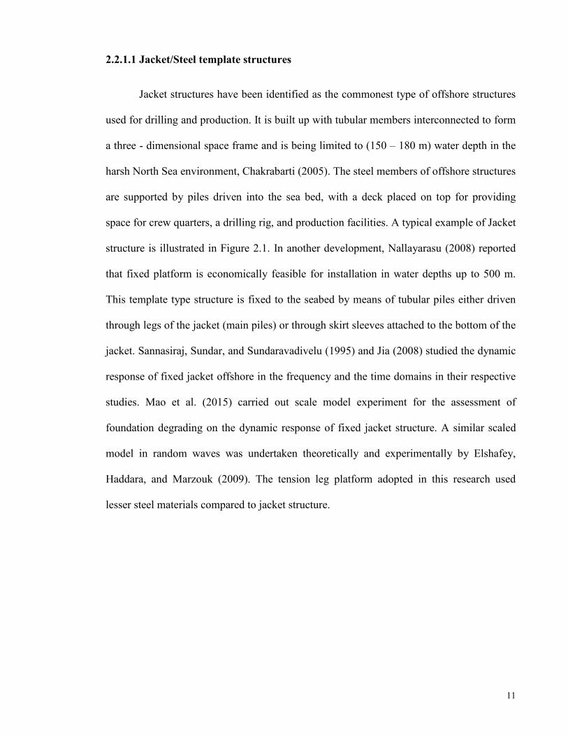
17
are prohibitively high. Nallayarasu (2008), attested that guyed tower has been identified as
the development on compliant tower due to the anchor lines that are used to tie the tower to
the seabed. The displacement of the platform is controlled by the tension in the guy ropes.
Figure 2.6: Guyed tower platform
2.2.3 Floating structures
Floating structures can either be neutrally or positively buoyant structures. Examples of
neutrally buoyant structure include Spars, Semi-submersible, Floating Production System
(FPS), Floating Production, Storage and Offloading System (FPSO), whereas the buoyant
tower and the TLP are examples of a positively buoyant structure. The buoyancy force
plays an important role in carrying the deck load. Figure 2.7 shows various types of
floating structures found on the subsea. It should be noted that the response of floating
structures to wave, current and wind is dynamic and complicated in nature.

18
Figure 2.7: Floating structures
2.2.3.1 Floating Production System
Nallayarasu (2008) described floating production system (FPS) to be suitable for a
deep-water depth ranging between 600 m and 2500 m. The FPS has drilling and production
gadgets embedded inside the semi-submersible unit. The wire rope and chain are anchoring
elements that keep the system in place. This can also be achieved dynamically by using
rotating thrusters.
2.2.3.2 Floating Production, Storage and offloading System
In Nallayarasu (2008), Floating Production, Storage and Offloading System, FPSO
is made up of large tanker type vessel. By design, FPSO has capacity to process and store
production from not distant subsea wells to a smaller shuttle tanker. This is then conveyed
by the tanker to the onshore for further processing.

19
2.2.3.3 Tension Leg Platform (TLP)
Veritas (2012) defined tension leg platform as the floating structure that is
connected to the seabed through the tendon legs system. The manuscript reported that
tendons are pre-tensioned, stiff in axial direction to constrain vertical TLP responses to
very small amplitude. In another attempt,Veritas (2008) described the TLP as a positive
buoyant unit connected to a fixed foundation or piles by pre-tensioned tendons. The TLP
hull is made up of buoyant structural columns; pontoons and intermediate structural
bracings. According to Veritas (2012), the TLP can be classified into various groupings as
highlighted in the following section.
2.2.3.3 (a) Conventional TLP
This is a traditional design that follows the principle of column-stabilized units with
four columns, four pontoons and a top tension connector either on the tension porches or
inside the column. Examples of this type of TLP include Conoco Hutton, Auger and Mars
TLPs. D'Souza, Aggarwal, and Basu (2013) reported that production risers are normally
arranged at the middle of the platform deck. Figure 2.8 shows a typical hull configuration
of the conventional TLP and this type of TLP is considered for the analysis in this thesis.
Figure 2.8: Hull configuration of Conventional TLP

20
2.2.3.3. (b) Extended TLP
This type of TLP design is known to have smaller columns located in its inboard
and extended pontoons. Here, the tendons are connected to the extreme part of the pontoon.
Typical examples include KIZOMBA A, KIZOMBA B, and MAGNOLIA TLPs designed
by ABB Lummus Global. It is reported in D'Souza et al. (2013) that topsides can be
integrated quayside or in a drydock by heavy lift cranes. An extended tension leg platform
is shown in Figure 2.9.
Figure 2.9: Hull configuration of Extended TLP
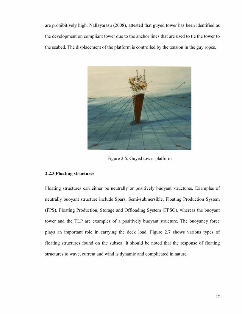
2.2.3.3 (c) SeaStar TLP
This is one of the newer concepts of TLP with only one central column and at least
three cantilevered pontoons projecting from the column base to the tendon porches for easy
connection of tendons. Examples of this type are the MATTERHORN and ALLEGHENY
TLPs designed by Atlanta sea-star. Figure 2.10 shows the hull configuration of SeaStar
TLP
21
Figure 2.10: Hull configuration of SeaStar TLP
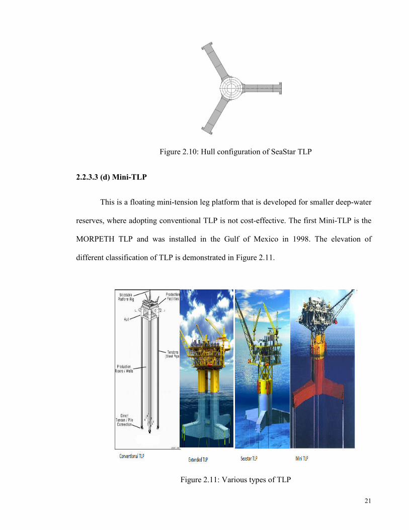
2.2.3.3 (d) Mini-TLP
This is a floating mini-tension leg platform that is developed for smaller deep-water
reserves, where adopting conventional TLP is not cost-effective. The first Mini-TLP is the
MORPETH TLP and was installed in the Gulf of Mexico in 1998. The elevation of
different classification of TLP is demonstrated in Figure 2.11.
Figure 2.11: Various types of TLP

22
Since the first TLP installation up till now, TLP has been tremendously use across
the oil producing fields including the Gulf of Mexico, North Sea, West Africa and Asia
countries. As of today, there are about twenty-eight installed TLP in various ocean fields
across the globe and in different water depths with varied construction materials and
operating in different environmental loadings. The progression of the existing TLPs and
their current status is given in Table 2.1.
In Table 2.2, technology of the each TLP with the numbers, sizes of their respective
tendons, tendon connection type and foundations are stated. Two of out of these platforms,
Hutton and Typhoon TLPs have been de-commissioned. The world’s largest TLP is the
HEIDRUN TLP located in Norway with the hull made up of concrete while the world’s
deepest TLP is Big boot TLP in GOM, Offshore Magazine (2010) and D'Souza et al.
(2013). The Riser-less Malaysian TLP started production in late 2016. The application of
TLP according to Veritas (2008) includes the exploration, production and storage of
hydrocarbons. In D'Souza et al. (2013), TLP is found suitable in production with full
drilling capability and dry trees, production with light intervention capability and trees,
production with dry trees, well head with tender or full drilling and dry trees.

23
Table 2.1: List of existing TLPs with their characteristics D'Souza et al. (2013)
No Field Operator Year
installed Location Water Depth
(m) Displacement
(Tons) Hull type Topsides function
1 Hutton Conoco 1984 North Sea 148 69,788 6-col hull DDP(8)
2 Jolliet Conoco 1989 GOM 536 18,302 4-col hull DWOW(9)
3 Snorre Saga 1992 North Sea 320 117,416 4-col hull DDP
4 Auger Shell 1994 GOM 872 72,986 4-col hull DDP
5 Heidrun Conoco 1995 North Sea 346 320,056
Concrete hull DDP
6 Mars Shell 1996 GOM 896 54,133 CTLP(3) DDP
7 Ram/Powell Shell 1997 GOM 980 54,133 CTLP DDP
8 Morpeth British Borneo 1998 GOM 509 11,687 SeaStar(4) WP(10)
9 Marlin BP 1999 GOM 988 26,460 CTLP DWOW
10 Allegheny British Borneo 1999 GOM 1004 11,687 SeaStar WP
11 Ursa Shell 1999 GOM 1204 98,497 CTLP DDP
12 Typhoon Chevron 2001 GOM 639 13,395 SeaStar WP
13 Brutus Shell 2001 GOM 910 54,684 CTLP DDP
14 Prince El Paso 2001 GOM 442 14,443 MOSES(5) DWOP(11)
15 Matterhorn Total 2003 GOM 869 26,405 SeaStar DWOP
16 West Seno A Unocal 2003 Indonesia 975 25,468 CTLP DTADW(12)
17 Marco Polo Anadarko 2004 GOM 1311 27,563 MOSES DWOP
18 Kizomba A Exxon-Mobil 2004 Angola 1200 35,280 ETLP(6) DDW(13)
19 Magnolia Conoco 2004 GOM 1425 34,398 ETLP DWOP
20 Kizomba B Exxon-Mobil 2005 Angola 1015 33,075 ETLP DDW
21 Okume Hess 2006 Equ.
Guinea 500 11,025 SSIP(7) DTADW
22 Oveng Hess 2006 Equ.
Guinea 280 11,025 SSIP DTADW
23 Neptune BHP 2007 GOM 1295 27,011 SeaStar WP
24 Shenzi BHP 2009 GOM 1333 43,439 MOSES WP
25 Papa Terra PetroBras 2013 Brazil 1180 44,817 ETLP DTADW
26 Big Foot Chevron 2014 GOM 1585 120,614 ETLP DDP
27 Olympus Shell 2015 GOM 919 54,023 CTLP DDP
28 Malikai Shell 2016 Malaysia 500 26,000
Notes
(1) Operator during construction phase (8) DDP = Dry Tree, Drilling, Production (2) Peak production during operation (9) DWOW = Dry Tree, Workover, Wellhead (3) CTLP = Conventional four column TLP (10) WP = Wet Tree, Production
(4) SeaStar = Mono Column TLP by SBM/Atlanta (11) DWOP = Dry Tree, Workover, Production
(5) MOSES =Multi Column TLP by MODEC (12) DTADW = Dry Tree, Tender Assist, Drilling, Wellhead
(6) ETLP =Extended TLP by Floatec (13) DDW = Dry Tree, Drilling, Wellhead
(7) SSIP = Self stable Integrated Platform by MODEC

24
Table 2.2: Progression and evolution of TLP technology, D'Souza et al. (2013)
No Field
Year Installed Tendon Technology
Water depth (m)
Nos of tendons
Tendon dia X WT (Inch)
Tendon connection type
Foundation type and size
1 Hutton 1984 First TLP with machined forging elements with threaded 148 16
10.23 (machined Threaded
Pile foundation templates
ends (this design is also classed as solid with central
forging) & 16.5 at connection
(4 no.); 8 piles/template;
hollow core for inspection) connectors w/ 3"
Spacer frame for
Tendons transported within the hull columns bored hole positioning
Tendons connected at bottom of hull columns
Collet type connector at bottom end
2 Jolliet 1989 Single piece thin walled tubular, welded 536 12 24 x 0.812 Welded &
Single template (200' x
One piece towed tendons towed tendon
200'); 16 main piles (60"
Installed after the TLP hull arrived at side design
x 300'); 4 leveling piles
Tendons connected to the porches outside of hull by pull (60" x 275')
in clamps; tendon in-situ inspection system
3 Snorre 1992 Steel tubulars with threaded connections, transported 320 16 32 x 1.5 Threaded
Concrete foundation
within hull columns connection templates (4 no., 5,700 st
Installed with bayonet connection with flex element for
each) w/skirts & solid
bottom end ballast
4 Auger 1994 Stabbed connection (box and pin Hunting connectors) for 872 12 26 x 1.3
Stabbed box
Pile foundation templates
tubular pipe sections done in SSCV and pin (4 no.);
Additional lateral mooring for positioning the TLP for Hunting
16 driven pipe piles (72" x
drilling operations connection 427' long)
5 Heidrun 1995 Single piece installation of towed tendons 346 16 44 x 1.5 Welded &
Concrete foundation
Tendons pre-installed with temporary buoyancy at top towed
templates w/skirts (4 no.,
tendons 22,500 st each)
6 Mars 1996 Tendons pre-assembled and hung-off at the installation 896 12 28 x 1.2 Merlin
1 driven pipe pile/tendon
vessel 12 piles (84" x 375')
TLP hull moored to the stern of installation vessel and
tendons passed over to hung-off the TLP hull
7 Ram Powell 1997 - 980 12 28 x 1.2 Merlin 84" x 349'
8 Morpeth 1998 First SeaStar TLP design 509 6 26 x 0.881 Merlin 84" x 318'
Pre-installed tendons w/temporary buoyancy
9 Marlin 1999 - 988 8 28 x 1.15 Merlin 84"
10 Allegheny 1999 - 1,004 6 28 x 0.949/1.02 Merlin 84"
11 Ursa 1999 Maximum water depth (4,000 ft) for TLP tendons and 1,204 16 32 x 1.5 Merlin 96" x 440'
foundation with available installation equipment in 1999

25
Table 2.2, Continued
No Field
Year Installed Tendon Technology
Water depth (m)
Nos of tendons
Tendon dia X WT (Inch)
Tendon connection type
Foundation type and size
12 Typhoon 2001 - 639 6 26 x 0.881 Merlin 84"
13 Brutus 2001 - 910 12 32 x 1.25 Merlin 82" x 340'
14 Prince 2001 First Moses TLP design 442 8 24 x 0.812 Merlin 64" x 320'
TLP designed for relocation in 6,000 ft water depth
15 Matterhorn 2003 First SeaStar TLP design with TTRs 869 6
32 x 1.143 Merlin 96" x 411'
Fairings on upper 1,100 ft of tendon length to reduce VIV
response in currents
16 West Seno A 2003
First TLP tendons fabricated outside USA and in Asia 975 8 26 x 1.06 Merlin 72" x 251'
Installation by a small vessel
17 Marco Polo 2004
TLP design in deepest water depth in 2003 1,311 8
28 x 1.1/1.2 Merlin 76" x 390'
18 Kizomba A 2004
First ETLP design & offshore Angola 1,200 8 32 x 1.4 Merlin 84"
19 Magnolia 2004 First stepped tendon design extending TLP WD limit to 1,425 8
32 x 1.42/1.5 & Merlin 96" x 313'
4,700 ft and beyond 40 x 1.19/1.32
Evaluated alternative
Menck to procure additional umbilicals to enable do pile
foundation designs
driving beyond 4,000 ft
Evaluated alternative composite tendon design
20 Kizomba B 2005 Design 1 Build 2 TLP case 1,015 8 32 x 1.4 Merlin 84"
21 Okume 2006 First SSIP hull design, offshore Equatorial Guinea 500 8
24 x 0.812 Merlin 64" x 198'
22 Oveng 2006 - 280 8 24 x 0.812 Merlin 64" x 173'
23 Neptune 2007 - 1,295 6 36 x 1.36 to 1.5 Merlin 96" x 414'
24 Shenzi 2009 Maximum design tension for a tendon and its connectors 1,333 8
36 x 1.55 & Merlin NA
Stepped tendon design 44 x 1.33/1.44
25 Papa Terra 2013 First TLP offshore Brazil 1,180 NA NA Merlin NA
26 Big Foot 2014 Deepest water depth with large dia stepped tendons 1585 16 36 / 44 Merlin NA
Heavy payload TLP
27 Olympus 2015 Largest tendons ever built for a TLP 919 16 38 x 1.44 Merlin NA
28 Malikai 2016
First TLP in Malaysia and third deep water project after Kikeh and Gumusut Kakap project 500

26
2.3 Advantages of tension leg platform
Tension leg platform is advantageous in deep water, and over other fixed and floating
platform due to the following reasons:
The amount of materials required is lesser compared to other floating structures
since it is the only the hull that uses most of the material and this makes it cost-
effective
TLP is a compliant structure capable of avoiding exciting wave frequency due to its
configuration
It requires lesser manufacturing and installation time in deep water
It accommodates both dry and wet trees and easy monitoring of risers and tendons
It is suitable for deep water and harsh environments
2.4 Environmental forces on tension leg platform
This can be defined as the loads resulting from the actions of environment. They
include waves, wind, current, ice and snow, earthquake, tidal effects, marine growth,
scouring and other seabed instabilities.
2.4.1 Wave forces
According to American Petroleum Institute (2001), wind-driven waves are the
major sources of environmental forces on tension leg platform. Such waves can be
modelled as either regular or irregular in shape. The ocean waves can vary in height,
length, and period, and may approach the TLP from one or more directions simultaneously.
The effect of modelling waves as regular and irregular waves is considered in this work.

27
2.4.2 Wind forces
Wind loading is important for accurate prediction of the global motion response of
floaters. Accurate modelling of the wind effects on the TLP is therefore essential. This
largely depends on the location and exposed area of the TLP. Wind load can be a
dominating excitation depending on location. The global wind loads acting on a floating
structure consists of two components, a static part resulting in a mean offset and mean tilt,
and a fluctuating component due to wind gusts which mainly excite the low frequency
motions in surge, sway and yaw. For some floater concepts, roll and pitch motions are also
influenced, Veritas (2012). The mean and fluctuating wind components are modelled for
the TLP in this study.
2.4.3 Current forces
Current is a constant motion of water that can emanate from wind-drag, tidal, and
background circulation components. In deep-water, it has been noted that current force
might produce large system loads. Current data is expected to be established for the site and
included in the design criteria. Near boundary currents (e.g., the Gulf stream, meanders,
and eddies) should also be considered. The current profile throughout the water column and
current scatter diagram should be determined, American Petroleum Institute (2001). The
current force co-exists with hydrodynamic force from wave motion in an ocean
environment. Generally, variations of tidal current force is normally governed by power
law and wind-drift current is usually modelled with linear profile, Dawson (1983). The
wind-drift current force is simulated in this study by adding the horizontal current velocity
to the horizontal water velocity caused by wave in the Morison equation.
28
2.4.4 Earthquakes
Earthquakes give rise to dynamic loads that have a high potential for disastrous
consequences for structures, as well as humans. There are different ways in which
structures are affected by earthquakes, the vibration of the ground being the most common,
but not the only one. Other earthquake effects are ground failures such as liquefaction (loss
of strength in silt or sand layers due to build-up of pore water pressure), landslides and
mudflows (usually triggered by liquefaction); further effects include sea waves (tsunamis)
and lake waves, Kappos (2002)
2.5 Wave theory
The wave theory is essential for the design of offshore structures. Although, the
assumption for formulation of wave theory is regular, the theory has been extended to
realistic random waves. This implies that a regular wave has the same form for the cycles.
With the wave height, wave period and depth of water known, it is possible to determine
the wave profile, water wave velocities and accelerations. The following section describes
some of the available wave theories.
2.5.1 Linear wave theory
In the work of Chakrabarti (2005), wind action on the ocean create a motion and
this is normally brought back to the calmness by the action of gravity and the outcome of
this disturbance is regarded as wind generated gravity waves. Linear wave theory is
formulated with the assumption that velocity potential depends on the position and time.
The wave height is assumed small compared to the wavelength and water depth. The
velocity potential is made to satisfy Laplace equation, linearized form of Bernoulli’s
dynamic equation and boundary conditions at the free and bottom surfaces. The solution of

29
the velocity potential give rise to fluid kinematics that are employed for the calculation of
wave-induced forces on the platform, Wilson (2003)
2.5.2 Stokes wave theory
This theory is formulated by modelling velocity potential and wave elevation with
perturbation parameters. These parameters can be extended to any order so as to obtain
wave theory. The assumptions used in the theory is that fluid is inviscid and
incompressible. The fluid particle velocities and accelerations can then be calculated from
velocity potential. The advantage of stoke wave theory is that the fluid kinematics are
calculated up to the instantaneous fluid level for all values of time.
2.5.3 Stream function theory
Unlike linear wave theory, Chakrabarti (2005) defined stream function theory as a
nonlinear wave theory which can either be regular or irregular stream function theory. The
regular stream function theory is formulated using wave parameters of wave height, wave
period and water depth. The irregular stream function theory is not limited by the wave
form of horizontal or vertical symmetry as it is the case for regular type. This theory is
normally being applied where free surface wave elevation or wave basin data are available.
2.5.4 Numerical theory
Numerical wave theory gained popularity as a result of introduction of sophisticated
computers with high speed. The theory is based on deterministic solutions of the governing
equations of the flow field. The assumption for the fluid in this theory include non-viscous,
irrotational and incompressibility properties of the fluid. The governing equation is solved
in terms of stream function. The theory has been applicable for deep-water waves, shallow
waters where linear wave theory is not suitable as well as nonsymmetrical waves.
30
2.6 Dynamic analysis of tension leg platform
Veritas (2008) revealed that the time domain approach is beneficial for global
motion response analyses because it is possible to include all environmental load effects
and typical nonlinear effects such as hull drag forces (including relative velocities), finite
wave amplitude effects and non-linear restoring functions from tendon and risers. The
frequency domain motion analysis has been identified by as the basis for generating
transfer functions for frequency dependent first and second order excitation forces, added
mass and damping (potential & viscous). It might also be possible to work with motion
response amplitude operators, but this is considered more cumbersome when transferring
into the time domain. The frequency domain analysis is capable of solving the equations of
motions for each of the incoming regular wave components for a wave frequency analysis,
and for each of the sum or difference- frequency combinations for a second-order analysis
(high- or low frequency response). The output from a traditional radiation/diffraction
frequency domain analysis is typically the excitation forces/moments, added mass/moments
and potential damping and motion RAOs.
2.6.1 Time and Frequency domain analyses
In Garrett (2005), procedures for the time and frequency domain analyses were
given for floating production system. The vessel was idealized as rigid body while mooring
lines and risers were modelled as slender elastic rods; these are all coupled together with
connecting link. The frequency solution was formulated for nonlinear static and harmonic
loads while nonlinear dynamic problem was fully coupled for floating production system in
the time domain. Correa, Jacob, and Mansur (2010) presented a hybrid time-frequency
approach for the solution of dynamic problems in order to overcome long time simulation
31
and also preserve nonlinearities in the system. Low (2009) carried out statistical
linearization for the tendon restoring forces in six degree of freedoms in order to overcome
high computational cost. The formulation in the frequency domain was said to include
nonlinear couplings. The reported results of the frequency and the time domain show some
level of agreement subject to certain conditions.
Lei et al. (2014) carried out lateral response analysis of floating production, drilling,
storage and offloading unit riser in the frequency domain. This was achieved by linearizing
the drag wave force. Low and Langley (2006) developed procedure for fully coupled
floating production system in the time and frequency domain. The two methods were
reported to have good comparison. Zou (2003) argued that dynamic interaction among the
TLP platform, tendons and risers cannot be fully captured using de-coupled analysis. The
study also reinstated that physical model tests are limited in terms of facilities and scaling
the model might lose the true representation of the platform. The study estimated the
hydrodynamic forces in the frequency domain and solved the problem in the time domain.
Masciola and Nahon (2008) employed the Newton and Euler equations of motion to model
the platform as rigid body in the six degree of freedoms and tendons are assumed as cables.
The first and second order wave forces were analytically developed in MATLAB and
solved by the Runge-Kutta method of numerical integration. Chitrapu and Ertekin (1995)
carried out numerical analysis of the TLP in the time domain. The equations of motion
were developed using the Newton- Euler approach; both the Morison and Potential theory
method were used for the computation of hydrodynamic forces. Ormberg, Baarholm, and
Stansberg (2003) argued that de-coupled analysis has the tendency to evaluating inertia
properties of the dynamical TLP model inconsistently due to the absence of real effective
mass that come from slender structures. The study employed WAMIT software for the
calculation of low, high and wave frequency excitation forces. RIFLEX-C and SIMO

32
software were used for coupled and de-coupled analysis in the time domain. The present
study formulated the problem in time-domain so as to include nonlinear effects from the
system and hydrodynamic force. The Newmark numerical method is employed for the
solution of the formulation.
2.7. Analysis of coupled and uncoupled of TLP models
This review opens with Morgan (1983) who developed a computer program that
calculate dynamic response for second order differential equation of motion for tension leg
platform. The equation of motion was formulated from nonlinear stiffness coefficients and
Morison’s equation and this was solved numerically using the Newmark beta-method.
Yoshida, Ozaki, and Oka (1984) studied the applicability of the linear response analysis
method for the tension leg platform. The study compared the proposed linear response with
small scale models and the results of structural response were validated. Jefferys and Patel
(1982) study reported that ignoring lateral tether dynamics can fairly estimate platform
motion but seriously impaired tether displacement. There is a wide range difference
between the natural frequencies of the platform and wave excitation frequencies from the
past study. However, the results of the TLP models show that in deep water, tether can
possess lateral resonant frequencies with the exciting wave frequency and this
correspondingly cause instability. This submission was verified to be true in this study.
Bar-Avi (1999) carried out nonlinear dynamic analysis of tension leg platform. The study
modelled the platform as rigid and tethers as flexible cables using beam continuous
systems. The response result from equation of motion was presented. Lyons and Patel
(1984) in an earlier study showed comparison of wave induced motion results of theoretical
and experimental tensioned buoyant platforms. Similarly, a close and good agreement was
33
reported for surge motions with magnitude discrepancies for tether tension at some wave
frequencies in Spanos and Agarwal (1984)
The state of art for the analysis of the TLP had always been undertaken either in
uncoupled or semi-coupled form. The procedures for uncoupled analysis as stipulated in
American Petroleum Institute (1996), Sen (2002), Chakrabarti (2008) involve analysis of
hydrodynamic floating structure for its motion while tendons were taken as external
nonlinear stiffness. This is followed by component analysis of mooring line and riser
individually. The floating structure motion can then be applied at the connection top points
together with the disturbed wave and current loads on the components solved by lumped
mass approach or finite element method. The mass and damping forces of the tendons are
always neglected in uncoupled analysis. Yang et al. (2014) identified the need for coupled
dynamic analysis of integrated platform and mooring lines. Both quasi-static and coupled
dynamic for truss Spar and mooring lines were developed in the time domain for irregular
waves. The coupling between the platform and mooring was achieved through appropriate
displacement and force boundary conditions. The hydrodynamic forces were calculated in
the time domain unlike in the method of using specialized software and doing transfer back
to the time domain as usually undertaken by previous researches. The effect of coupled
dynamic analysis of floater motions on the mooring and riser system response of a floating
production storage offloading was emphasized in Caire and Schiller (2012) to lower the
conservatism adopted in the current practice of fatigue assessment. Similarly, Ormberg and
Larsen (1998) illustrated that motions of platform in de-coupled analysis were modelled
and calculated by simplifying forces from the mooring and riser lines. This has traditionally
been followed with simulation of the platform motion as top end excitation in the
calculation of dynamic loads of the mooring lines and risers. The analysis in the time
domain was carried out with SIMO software and RIFLEX software was used for coupling

34
and modelling of floater and mooring lines together. Coupling effect between the floater
and mooring lines have been reported by Astrup, Nestegård, Ronæss, and Sødahl (2001) as
the influence on floater mean position and dynamic response due to slender restoring,
damping and inertia forces. The current practice by industry as reported by Caire and
Schiller (2012) was the de-coupled analysis. This is always achieved by excluding mooring
lines and tendons from the floater motion. Consequently, this is then imposed as the
external force during the dynamic analysis of the mooring line. Most hydrodynamic
software such as WAMIT, AQWA, HOBEM employ this methodology. Without fully
integrating the coupling between the floater and lines, the accuracy of the platform motion
may be undermined. Both coupled and uncoupled TLP models are modelled so as to assess
their behaviour in Abaqus/Aqua software.
Bhattacharyya et al. (2003), Chatterjee et al. (1996), Natvig and Johnsen (2000)
suggested that motion characteristics and structural response of compliant structures can be
better idealized as a coupled model using the finite element method. In another attempt,
Giron, Correa, and Jacob (2014) developed a hybrid semi-coupled model that combines the
features of coupled and de-coupled analysis for the floating production system. Le, Ding,
and Zhang (2014) discussed coupled motion characteristics of the floating mooring
platforms under regular and in a coupled model against the de-coupled analysis. The
agreement and differences between the de-coupled and coupled analysis results were
presented.
The need for coupled formulation was identified by Correa et al. (2002), which
simply implies that hydrodynamic model of the floating structure is coupled to the finite
element model of mooring and riser lines with mass and damping included. The equations
of motion must then be solved simultaneously. Adrezin et al. (1996) reported that tendons
were mostly modelled as massless springs in most studies but in advanced models, tendons

35
can be represented as beams, cables or springs with increased complexity. Due to the
extreme tension experienced by tendons in deep water with fluid flowing around them there
is a need to consider higher order effects in loading and structure.
Adrezin and Benaroya (1999a) employed extended Hamilton's approach to derive
sets of nonlinear equations for single tendon TLP. The Lagrangian approach was used to
develop energies on the tendons. The hull was represented as a rigid body and the system
simulated for random waves and current load. The Morison equation and the Pierson
Moskowitz spectrum were used for simulation of random sea. Results for the quarter ISSC
TLP was reported and for wave only, the TLP vibrates about vertical position and about
offset position when current force was added. Application of forces on tendons increases
amplitude and offset position as compared to when the forces were absent.
In another paper, Adrezin and Benaroya (1999b) derived sets of equation of motion
for the calculation of surge and pitch responses for the hull as well as the surge response
along the tendon. Ahmad, Islam, and Ali (1997) investigated the response of the TLP when
excited by wind forces in the time domain. The Simiu’s spectrum was adopted for this
problem and major nonlinearities as considered earlier in Ahmad (1996) were also
incorporated. The effects of mean wind and fluctuating wind over random wave simulation
in coupled and uncoupled motion were examined. The response of the TLP to wind-
induced load found that surge and yaw responses were greatly affected by the intensity of
the wind force, however, the magnitude of pitch and roll were not pronounced due to
vertical restraints.
2.8 Finite element modelling of TLP
Jayalekshmi et al. (2010) studied the behaviour of TLP in random waves. Pierson–
Moskowitz, (PM) spectrum was used to simulate time history of random waves of TLP

36
with and without risers under the action of random waves and current. The response
spectral densities were reported to be significantly reduced and this was attributed to the
riser hydrodynamic damping related to the riser drag. There was an increase in the offset
and set-down values due to the nonlinearities that arise from steady current drag on the
risers and wave drift force. Joseph, Mangal, and George (2009) used finite element
numerical for the analysis of a 3- column mini TLP and compared their result with a 4-
column mini TLP. It was reported that dynamic responses were close to a 4-column mini
TLP with relatively high surge and tendon variation. Zou (2003) carried out coupled
dynamic analysis of the hull, tendon and riser and reported that up-wave and down-wave
tendon tensions do exist even though static offset and set-down of coupled and uncoupled
agreed.
Bachynski and Moan (2012) employed the concept of TLP for wind turbine in
accessing offshore wind resources under different wave –wind conditions. The JONSWAP
and Kaimal spectra were used for the simulation of random waves and fluctuating wind.
Parametric studies were carried out on a single column tension leg platform wind turbine.
This was followed by the evaluation of platform motions and structural loads on the turbine
components and tendons. Commercial aero- and- hydrodynamic software were used for the
analysis and design. It was reported that the presence of wind turbine on the TLP platform
showed no large effect on the turbine blade but rather causes an increase in variation of the
bending moment at the base when compared with land based turbine. Bhattacharyya et al.
(2003) conducted nonlinear dynamic analysis of the Sea-Star mini TLP using the finite
element method coded in FORTRAN. Based on the comparison between the experimental
and numerical, it was recommended that the result of the finite element procedure can be
relied upon. The same principle of general finite element method is used for model
discretization in Abaqus/Aqua in this study.

37
2.9 Different analysis method and load combinations
Liu (2014) carried out a parametric study of the TLP under varying incident wave
angles, wave heights and wave periods. It was reported that these parameters had little
effect on the tension variation. However, the increase in the wave period increases the
surge position, and decreases the heave, roll and pitch. Also, the wave height effect was
minimal on heave but more on other degrees of freedom. In another similar work, the
radiation/diffraction theory with the boundary element method was employed by Gao et al.
(2013) to compute motion responses and wave forces on floating TLP wind turbine. Their
findings show that the maximum response of sway and the minimum response of surge
have the same direction. It was the same with the maximum response of pitch and the
minimum response of roll. Again, motion responses of heave and yaw did not acutely
change as the other four directions did. Kareem and Li (1993) presented a frequency
domain analysis procedure in the evaluation of wind excited surge response of a TLP in the
presence of wave and currents. Vickery (1995) and Ahmad et al. (1997) examined the
combined effect of wind and wave loads on the response of the TLP. An agreement
between the theoretical results and experimental findings was established. Chandrasekaran
and Gaurav (2008) analysed non-linear dynamic equations of motion for a triangular
tension leg platform at different water depths operating under the high sea waves and
earthquake motion. Similarly, Chandrasekaran et al. (2004) studied the influence of
hydrodynamic drag coefficient and hydrodynamic inertia coefficient on the non-linear
response behaviour of two different tension leg platform models operating under regular
waves. It was reported that constant coefficient throughout the water depth yielded higher
motion response compared to the results from varying the coefficients. Muhittin and Oguz

38
(2003) analysed motion of platform by both single-wave prediction and spectral method
and found the latter produced more favourable results.
Chandrasekaran, Jain, Gupta, and Srivastava (2007) reported results for two
triangular TLP operated under the combined action of regular wave and impact loadings. It
was concluded that the platform was affected when the impact was on the corner column
and that the impact on the pontoon seems not to affect the platform. Chandrasekaran and
Jain (2002b) also, reported that heave and surge responses of square TLP was higher than
that of triangular TLP but the pitch degree of freedom attracted more forces due to the
pontoons arrangement to the unidirectional wave. A similar work by Tabeshpour,
Golafshani, and Seif (2006) made use of simple stable numerical integration known as the
Modified Euler Method (MEM) for the analysis of the dynamic response of structures in
the time domain. In their study, the stability of the method for solving differential equation
of motion of a nonlinear TLP offshore system in random wave excitation was presented.
The key point of suitability of the MEM for solving the TLP system was that the maximum
frequency of the system is about 0.5Hz. The stability criterion and the convergence of the
numerical solution for critical time steps were numerically discussed.
Ahmad (1996) carried out an analysis of stochastic response of TLP in the time
domain under long crested random sea. The stiffness coefficients for square tension leg
platform were developed for coupled motion in six degrees of freedom. The result of
stochastic response was summarized in statistical forms. The study concluded that
geometry characteristics, angle of incidence, variable submergence, current velocity and
tether tension affect the dynamic response of the TLP to the random wave and currents.
Siddiqui and Ahmad (2003) studied the response behaviour of tension leg platforms under
impulsive forces. Siddiqui and Ahmad (2000) carried out a reliability analysis of an intact
and one tether missing tension leg platform in various sea conditions. The focus of their

39
paper was on annual and life time probability of other tethers when one tether is missing or
broken under regular wave, regular wave and wind and long crested seas due to maximum
and minimum tension in the cable. Amanullah, Siddiqui, Umar, and Abbas (2002) studied
the reliability of tension leg platforms against various limit states of failure. Khan, Siddiqui,
Naqvi, and Ahmad (2006) examined the reliability behaviour of tether to derived limit state
maximum tension under action of wave and impulsive load. The sensitivity of the random
variables on reliability was also undertaken. Ardakani and Ketabdari (2007) presented the
results of experimental work performed on a scaled model for the Sea-star TLP in a wave
flume.
Hydrodynamic responses analysis of tension leg platform was investigated by Chen
et al. (2013). The modelling of their platform was performed using the DNV/SESAM
software. The study carried out the optimization of wave direction and period that gave
worst motion responses in both frequency and in the time domain. Lee and Wang (2000)
investigated the surge response of tension-leg twins platform. The equations were derived
and the effects of reflection coefficient and dimensions of the platform on the response
were also studied. Chandak and Chandrasekaran (2010) investigated response the
behaviour of TLP with triangular geometry using the dynamic Morison equation.
Nonlinearities associated with vortex shedding effects were considered along with standard
Morison equation. Rudman and Cleary (2013) used smoothed particle hydrodynamics to
simulate large waves on tension leg platform. The platform motions and tensions in the
cable were investigated to the effects of wave impact angle and mooring line pretension.
Tabeshpour and Shoghi (2014) carried out solution for surge motion of TLP with the
homotropy perturbation method. Karlinsky and Kuteynikov (2008) proposed formulas and
presented result for ice resistant TLP. It was concluded that the stability requirement of the
ice-resistant TLP has to be different from the normal floating TLP. Similarly, Chernetsov
40
and Karlinsky (2006) analyzed four platform floating substructures. Two of the platforms
were Spar-type, whereas the other two was of TLP-type structure in ice middle sea depth.
Rijken and Leverette (2007) reported that the dynamic tension levels resulting from
earthquake near the tension leg platform in the Gulf of Mexico are minor and are far less
than the extreme tensions under storm and hurricane conditions.
Kim et al. (2007) conducted a dynamic response analysis of tension leg platforms
including hydrodynamic interaction in regular waves. The study assumed the whole
structure as flexible and used a numerical method based on a combination of three-
dimensional source distribution and dynamic structural analysis method for the analysis.
Chandrasekaran and Jain (2002b) investigated the dynamic response of a triangular
configuration Tension Leg Platform (TLP) under random sea wave loads. The random
wave was generated synthetically using the Monte-Carlo simulation with the Pierson–
Moskowitz (P–M) spectrum. The effect of the coupling of various structural degrees-of-
freedom on the dynamic response of the TLP under random wave loads was also studied.
The paper concluded that in the presence of current, the response behaviour of the TLP was
altered significantly introducing a nonzero mean response in all degrees-of-freedom.
Kurian et al. (2008) developed a MATLAB computer program for determining the dynamic
responses of square TLPs subjected to regular and random waves. The structure was treated
as a rigid body and all the six motions as well as the tether tensions were determined. The
linear Airy wave theory and the Morison equation were used for wave force calculations.
The equation of motion was organised in MATLAB and the Newmark Beta numerical
integration method was used for the time domain analysis. The response amplitude
operators for the motions of a typical TLP were compared with the available theoretical and
experimental results. Besides, parametric studies of different parameters such as water

41
depth, pretension, wave angle and position of center of gravity (CG) were also undertaken.
The work reported results of platform responses caused by varying these parameters.
Li and Kareem (1990) researched on the dynamic behaviour of tension leg
platforms (TLPs) under the simultaneous action of random wind and wave fields.
Computationally efficient time and the frequency domain analysis procedures were
developed to analyze the wind-wave- current-structure interaction problems. The
aerodynamic load effects were described by the space-time description of the random wind
field. The hydrodynamic loads were expressed in terms of a combination of viscous and
potential effects. A stochastic decomposition technique was developed which significantly
enhanced the efficiency of the frequency domain analysis of complex systems. A
numerical scheme involving iterative and perturbation techniques was utilized to evaluate
the second order response statistics. The response of a typical TLP in six degrees of
freedom showed excellent agreement between the time and frequency domain analyses.
Chandrasekaran, Jain, and Chandak (2006) analysed the nonlinearities due to the change in
tether tension and nonlinear hydrodynamic drag forces. The coupled response of TLP under
moderate regular sea waves due to the change in initial pretension in the tethers caused by
seismic forces was then investigated. Seismic forces were imposed at the bottom of each
tether as axial forces. The tether tension becomes unbalanced when the hull was under
offset position. The change in initial pretension due to the vertical component of the
earthquake influenced the response of the triangular TLP in degrees-of-freedom
experiencing such forces. The tether tension varied nonlinearly when the platform was
subjected to seismic forces caused by the El-Centro earthquake and artificially generated
earthquake using the Kanai–Tajimi’s power spectrum. The response due to earthquakes
varied with the intensity of the input ground motion. Naess, Gaidai, and Teigen (2007)
carried out an analysis for TLP in first order, second order wave frequency and slow-drift
42
motions. The analysis predicted results for extreme response statistics of the horizontal
surge motions. Masciola and Nahon (2008) presented a non-linear six degree-of-freedom
dynamics model results for a tension leg platform type structure. The dynamics model and
simulation presented was different from other previous models in the derivation approach.
Existing models were usually based on deriving stiffness coefficients from an analysis of
single-degree-of-freedom perturbations of the platform. Their study analysed the
generalized platform motion based on fundamental kinematic principles and calculate the
forces and moments resulting from this motion. Yongjun, Jiemin, and Qingyong (2008)
carried out a diffraction analysis of short-crested wave with uniform current. The study
reported that wave frequency was influenced by incident angle and strength of the current
velocity.
2.10 TLP-Tendon-Riser system
Mekha, Johson, and Roesset (1996) investigated the implications of tendon
modelling on TLP response by using constant lateral tendon stiffness, time varying axial
tendon stiffness and coupled analysis of hull and tendons. Also, Chandrasekaran, Chandak,
and Anupam (2006) reported that tension variation in the TLP tendon played a significant
role in its stability. Gadagi and Benaroya (2006) loaded a tether at the free end and subject
it to various end tensions. The parametric effect of harmonically varying the end tendon
brought an increase in the constant end tension. Results of the effect of different significant
wave heights on the axial and transverse motion were also presented. Aguiar, Almeida, and
Paulino (2014) formulated and implemented finite element modelling for Timoshenko
beams on multi-layered pipe beam element. Also, axial, bending and torsional degrees of
freedoms were included in the derivation. Jayalekshmi, Sundaravadivelu, and Idichandy
(2009) studied the effects of the dynamics of riser on TLP behaviour in nonlinear finite

43
element program for regular waves. It was reported that the riser effect reduced the
dynamic surge due to hydrodynamic damping from the riser and increase the mean drift
surge and set-down due to additional hydrodynamic forces and current forces. Islam,
Jameel, Ahmad, Jumaat, and Kurian (2013) carried out an analysis of coupled Spar-
mooring system using finite elements in Abaqus software. The environment was simulated
for severe sea states and the Morison equation was used for force computation. It was
reported that time histories of surge, heave, pitch and maximum mooring tension decreased
and remained steady after the transient state. Yang, Teng, Ning, and Shi (2012) analysed
the coupled dynamic response of truss Spar and its mooring line/riser in the time domain.
The analysis program for the equation of motion was developed and simultaneously solved
for truss Spar and mooring systems using the Newmark-β and Newton-Raphson iterations.
Bahtui, Alfano, Bahai, and Hosseini-Kordkheili (2010) adopted the finite element
formulation for a nonlinear analysis of flexible riser. The approach was based on the
incrementally updated Lagrangian together with the modified linearization scheme for the
analysis of annular section of 3-D beam element. The influence of buoyancy force and
current force were considered on the riser pipeline. Adamiec-Wojcik, Brzozowska, and
Drag (2015) derived set of formulas for the dynamic analysis of risers during vessel motion
using the modified rigid finite element that included bending and longitudinal deformations
of the planar slender links. Drag forces, uplift forces, sea currents and added mass
influences through the Morison equation were applied on the slender structures.
Jameel, Ahmad, Islam, and Jumaat (2014) analysed the motion response of the Spar
platform under wave and wind loading using the coupled model. It was reported that wind
induced forces affect mooring and motion response significantly. In another development,
Han and Benaroya (2002) formulated coupled nonlinear equation for axial and transverse
motion of a tower. The nonlinear free and forced responses were later compared with the
44
linear model. Khan et al. (2006) examined the reliability behaviour of tether to derive limit
state maximum tension under action of wave and impulsive load. The sensitivity of the
random variables on reliability was also undertaken. Chatterjee et al. (1996) studied the
hydrodynamic behaviour of the long floating structure and reported that as the mean wave
direction increases, the response ratio decreases. The increase in the spreading parameter
made the response of short-crested idealization closer to the long-crested sea state. More
recently, Ng, Kurian, and Liew (2014) examined the responses of the classic Spar in short
and long crested wave generation experimentally. Their study reported that the responses
from long-crested simulation were found to be thirty-five percent higher than those from
short-crested sea. Zaheer and Islam (2012) examined the response of an Articulated Leg
Platform (ALP) to wave alone, wind alone, and to correlated wind and waves. The
fluctuating component of the wind was modelled with different wind spectra while the sea
state was characterized by the Pierson–Moskowitz (P–M) spectrum. Their work
demonstrated that the Davenport wind spectrum response was lower as compared to other
spectra used. Bisht and Jain (1997) studied the response of guyed tower platform to random
wave and wind and came to the submission that wind forces increased the mean values of
the platform responses. The effects of the magnitudes and the directions of wave, wind,
current at different wave heights were simulated in the work Yilmaz and Incecik (1996b)
on moored floating platforms. The study concluded that the direction of wave incidence
and reduction in the number of mooring legs affect the motion of the system. Han and
Benaroya (2002) formulated a coupled nonlinear equation for the axial and transverse
motion of a tower. The nonlinear free and forced responses were later compared with the
linear model. Benfratello, Di Paola, and Spanos (1998) analysed the stochastic response of
multi degree of freedom of wind-excited structures by means of the Volterra series
approach and stated that computational effort of this method was lesser as compared to

45
earlier methods used for the computation of multiple integrals. Islam, Jameel, Jumaat,
Shirazi, and Salman (2012), Jameel et al. (2013), Mohd Zaki, Abu Hussain, and Najafian
(2014) studied the behaviour of the integrated Spar-mooring system under the actions of
wave, wind and current forces. Shehata and Raheem (2013) employed a finite element
analysis in determining the displacements and stresses in the steel jacket structure and the
results of the nonlinear analysis were presented for a safe platform operation. Barranco-
Cicilia, Lima, and Sagrilo (2008) presented the methodology to perform a Load and
Resistance Factor Design (LRFD) criterion for the design of Tension Leg Platform (TLP)
tendons in their intact condition.
2.11 Summary of previous works
From the foregoing, the bulk of the research in this area had traditionally been on
de-coupled analysis with limited works on semi-coupled in trying to bridge the gap
between the uncoupled and coupled analysis of the TLP due to the high computational cost
and analysis time involvement. In view of this, this study will consider both uncoupled and
coupled TLP models in regular and irregular seas. A mathematical numerical code was
formulated in FORTRAN for uncoupled model and the Abaqus finite element software
with Abaqus/Aqua module techniques were used for the discretization and application of
loads for coupled models. These are discussed in greater detail in the next chapter.

46
CHAPTER 3: METHODOLOGY
3.0 Introduction
As discussed in the previous chapter, the time domain numerical model is
developed for uncoupled and coupled TLP. The mass, stiffness and damping forces of the
TLP are calculated and balanced with the external exciting forces. The environmental
forces considered for this analysis include regular and random waves; current and wind
forces. The regular wave was simulated with the linear wave theory while random waves
were calculated through the Pierson-Moskowitz spectrum, followed by the calculation of
hydrodynamic forces with the Morison equation. Also, the current force was calculated by
adopting the linear current profile type of Veritas (2007). For the superstructure, the effects
of mean and fluctuating wind loads were calculated using Emil Simiu and API spectra
respectively. The TLP was assumed to be a small structure since the ratio for diffraction
parameter of characteristic dimension and wavelength is less than 0.2, hence wave
diffraction and radiation was neglected.
The present problem was solved using two different approaches. For the first
approach, equations of motion for the TLP were formulated from the first principle. Then
the equations of motion were coded and numerically solved in FORTRAN software
embedded with subroutines that calculate inertia, damping, restoring forces matrices as
well as the external forces vector on the TLP. The second method employed the Abaqus
finite element analysis software to model platform as rigid beams and tendons as finite
elements with proper connector to impose boundary conditions. The Abaqus/Aqua product
which was designed originally for application of hydrodynamic wave loading on offshore
pipelines, was used to apply hydrodynamic forces on the platform model and tendon legs.
47
Numerical model incorporates various degrees of nonlinearities on the TLP such as
variable submergence, added mass, drag force, tension fluctuation, and large displacement.
The equation of motion was formulated in an efficient manner and this was solved by using
the Newmark-βeta integration scheme. A numerical model known as the Uncoupled
Nonlinear Analysis Program (UNAP-TLP-2016) was developed and solved for uncoupled
TLP in FORTRAN. The solution of the coupled TLP system was successfully
accomplished by Abaqus finite element software and named as Coupled Nonlinear
Program (CNAP-TLP-2016).
3.1 TLP structural idealization and assumptions
For both uncoupled and coupled TLP models, a double symmetric rectangular ISSC
platform with four solid tendons at each corner was employed. The TLP structural
configuration adopted for this study is the International Ship and Offshore Structures
Congress (ISSC). Model geometry of this platform consists of four vertical cylindrical
columns and four horizontal pontoons with a group of tendons at each corner end. ISSC
sketch plan and elevation are shown in Figure 3.1 with other mechanical characteristics
outlined in Section 4.3. The basic differences between the coupled and uncoupled as it
affects the mathematical formulation is stated in Table 3.1
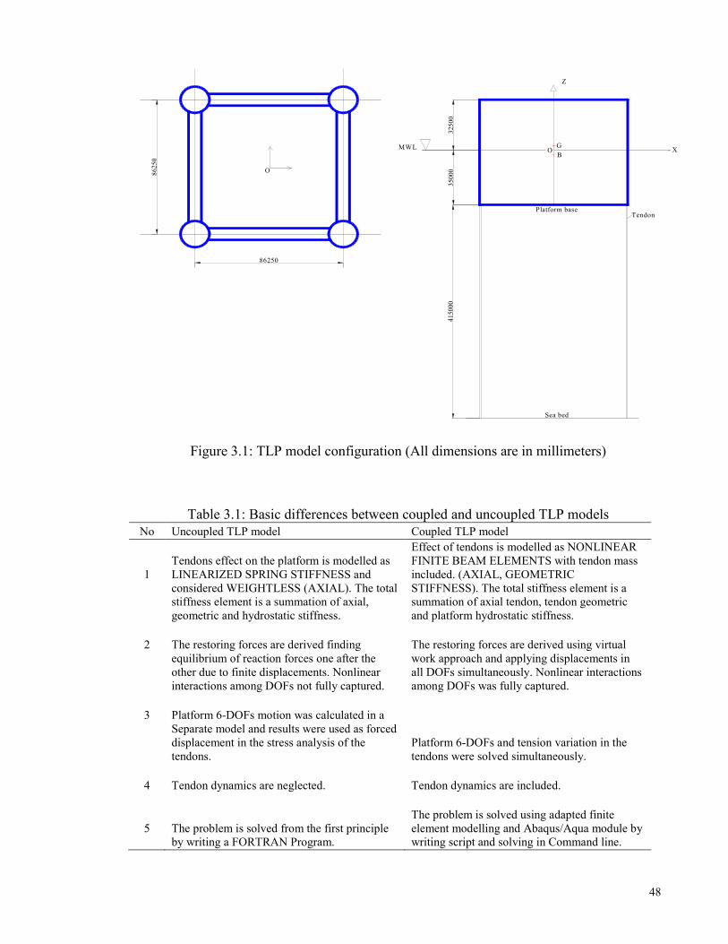
48
Figure 3.1: TLP model configuration (All dimensions are in millimeters)
Table 3.1: Basic differences between coupled and uncoupled TLP models No Uncoupled TLP model Coupled TLP model
1
Tendons effect on the platform is modelled as LINEARIZED SPRING STIFFNESS and considered WEIGHTLESS (AXIAL). The total stiffness element is a summation of axial, geometric and hydrostatic stiffness.
Effect of tendons is modelled as NONLINEAR FINITE BEAM ELEMENTS with tendon mass included. (AXIAL, GEOMETRIC STIFFNESS). The total stiffness element is a summation of axial tendon, tendon geometric and platform hydrostatic stiffness.
2
The restoring forces are derived finding equilibrium of reaction forces one after the other due to finite displacements. Nonlinear interactions among DOFs not fully captured.
The restoring forces are derived using virtual work approach and applying displacements in all DOFs simultaneously. Nonlinear interactions among DOFs was fully captured.
3
Platform 6-DOFs motion was calculated in a Separate model and results were used as forced displacement in the stress analysis of the tendons.
Platform 6-DOFs and tension variation in the tendons were solved simultaneously.
4 Tendon dynamics are neglected. Tendon dynamics are included.
5
The problem is solved from the first principle by writing a FORTRAN Program.
The problem is solved using adapted finite element modelling and Abaqus/Aqua module by writing script and solving in Command line.
86250
862
50
O
3500
032
500
4150
00
Z
XG
BO
Platform baseTendon
Sea bed
MWL

49
The following assumptions were adopted in the derivation of the mathematical model in
this research while some of the previous simplifications were avoided:
(1) The TLP was idealized as a rigid body, symmetrical about the x- and y- axes with
the centre of gravity taken as the origin.
(2) The motions of the platform were governed by three translational and three
rotational degrees of freedom at the platform centre of gravity as shown in Figure
3.2.
(3) Surge, sway, heave, roll, pitch and yaw motions were coupled together.
(4) The structural mass of the TLP and moment of inertia were lumped at the centre of
gravity.
(5) The tendons that anchor the TLP to the seabed were idealized as linear springs for
uncoupled TLP and hybrid beam elements for coupled TLP.
(6) Hydrodynamic loads on the platform were due to the gravity waves and current
forces while aerodynamic force was applied on the superstructure.
(7) The Morison empirical formula was adopted for wave induced forces with the
verification that sectional dimension was far less than wavelength hence diffraction
effect is ignored.
(8) The linear wave theory was employed for calculation of water particle velocity and
acceleration.
(9) The water was assumed inviscid, incompressible and the motion was irrotational.
(10) Gravity, inertia, hydrostatic and hydrodynamic forces were applied on the tendons
and connecting elements for the coupled model.
(11) Variable submergence and instantaneous buoyancy were active and significantly
influence the heave response of the TLP.
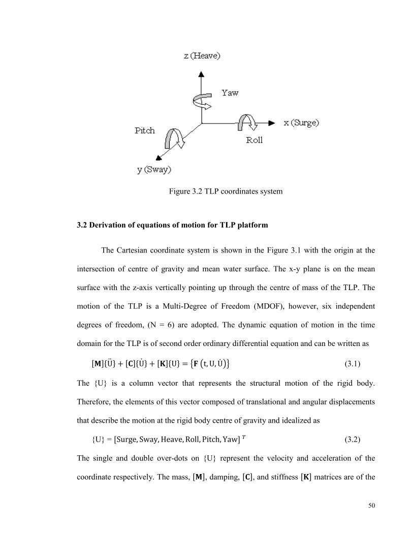
50
Figure 3.2 TLP coordinates system
3.2 Derivation of equations of motion for TLP platform
The Cartesian coordinate system is shown in the Figure 3.1 with the origin at the
intersection of centre of gravity and mean water surface. The x-y plane is on the mean
surface with the z-axis vertically pointing up through the centre of mass of the TLP. The
motion of the TLP is a Multi-Degree of Freedom (MDOF), however, six independent
degrees of freedom, (N = 6) are adopted. The dynamic equation of motion in the time
domain for the TLP is of second order ordinary differential equation and can be written as
[�]{U} + [�]{U} + [�]{U} = �� �t, U, U�� (3.1)
The {U} is a column vector that represents the structural motion of the rigid body.
Therefore, the elements of this vector composed of translational and angular displacements
that describe the motion at the rigid body centre of gravity and idealized as
{U} = [Surge, Sway, Heave, Roll, Pitch, Yaw] � (3.2)
The single and double over-dots on {U} represent the velocity and acceleration of the
coordinate respectively. The mass, [�], damping, [�], and stiffness [�] matrices are of the

51
order (N x N) and {� } is a (1x N) time-dependent column vector, these are discussed and
formulated in the following sections.
3.2.1 Mass matrix
With the assumption of the rigid body for the platform coupled and generalized
coordinates that defines the motion at the centre of gravity, lumped mass matrix approach
was adopted to calculate and allocate the mass along the degrees of freedom. The total
platform mass was lumped in surge, sway and heave directions. In respect to vertical
centerline, the structural mass was assumed to be symmetric and diagonal. The rest of the
three diagonal terms represent the mass moment of inertia due to the structural and added
mass with respect to roll, pitch and yaw degrees of freedom.
The total mass matrix is a summation of structural mass above the mean sea level
and fluid added mass as a result of accelerated motion of water around the TLP structural
members. The formulation for the constant added mass matrix was calculated as the
product of volume of the hull, water density and length of the hull. Thus, varying added
mass was considered as the product of body acceleration and mass quantity. Therefore,
elements of diagonal mass matrix were [M11 = M22 = M33 = M + Ma] along the surge, sway
and heave directions. [�] and ‘Ma’ are the total mass in the air and added mass
respectively. Similarly, the last three terms in the matrix were M44 = Mr�� + � �; M55
= Mr�� + � �, and M66 = Mr�
� + � � representing mass moment of inertia about the x, y
and z directions respectively. The ′ r�′, ′r�′ and ′r�′ were the radius of gyration about the x,
y and z directions. The fluctuating component of added mass due to variable submergence
was also included in the force vector of Equation 3.81.

52
[�] =
66
55
44
33
22
11
M
M
M
M
M
M
(3.3)
The unsteady motion flow around the TLP members created a force known as added mass.
This effect was considered in all forces associated with acceleration rather than along the
surge, sway and yaw only and they were lumped alongside with structural mass as shown
in Equation 3.81.
3.2.2 Damping matrix
Damping is the capability of a body to dissipate energy. Sources of damping include
structural, material and fluid for the type of floating body problems. The major source of
damping that was considered for this analysis was of the viscous effect type of fluid
damping due to the movement of fluid relative to the vibrating TLP. The structural
damping occurs as a result of friction among various parts of the body. Thus, structural
damping matrix, [�] in Equation 3.4 was defined to be a symmetric matrix of order (N x
N), degrees of freedom and proportional to mass and stiffness matrices
β[K]α[M][C] (3.4)
Where
α = alpha and β = Beta are Rayleigh constants calculated from modal damping ratio and
fixed for the dynamic system respectively. The nodal damping forces and nodal velocities
are related through a constant known as damping influence coefficient.
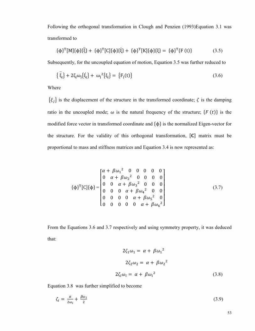
53
Following the orthogonal transformation in Clough and Penzien (1993)Equation 3.1 was
transformed to
{ϕ }�[M]{ϕ }{ξ} + {ϕ }�[C]{ϕ }{ξ} + {ϕ }�[K]{ϕ }{ξ} = {ϕ }�{F (t)} (3.5)
Subsequently, for the uncoupled equation of motion, Equation 3.5 was further reduced to
� ξ�� + 2ζ�ω ��ξ�� + ω �
��� = �F�(t)� (3.6)
Where
���� is the displacement of the structure in the transformed coordinate; � is the damping
ratio in the uncoupled mode; � is the natural frequency of the structure; {� (�)} is the
modified force vector in transformed coordinate and {ϕ } is the normalized Eigen-vector for
the structure. For the validity of this orthogonal transformation, [�] matrix must be
proportional to mass and stiffness matrices and Equation 3.4 is now represented as:
{ϕ }�[C]{ϕ } =
⎣⎢⎢⎢⎢⎢⎡� + ���
� 0 0 0 0 0
0 � + ���� 0 0 0 0
0 0 � + ���� 0 0 0
0 0 0 � + ���� 0 0
0 0 0 0 � + ���� 0
0 0 0 0 0 � + ���� ⎦
⎥⎥⎥⎥⎥⎤
(3.7)
From the Equations 3.6 and 3.7 respectively and using symmetry property, it was deduced
that:
2���� = � + ����
2���� = � + ����
2���� = � + ���� (3.8)
Equation 3.8 was further simplified to become
�� = �
�� �+
�� �
� (3.9)
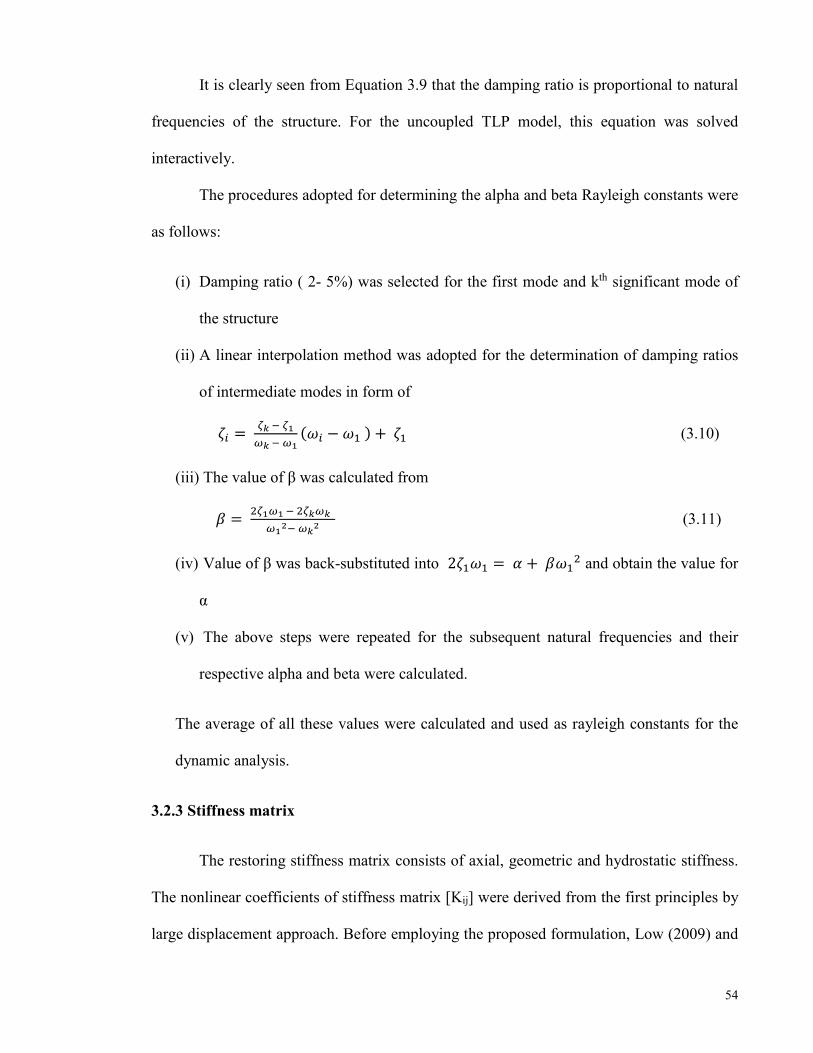
54
It is clearly seen from Equation 3.9 that the damping ratio is proportional to natural
frequencies of the structure. For the uncoupled TLP model, this equation was solved
interactively.
The procedures adopted for determining the alpha and beta Rayleigh constants were
as follows:
(i) Damping ratio ( 2- 5%) was selected for the first mode and kth significant mode of
the structure
(ii) A linear interpolation method was adopted for the determination of damping ratios
of intermediate modes in form of
�� = �� � ��
� � � � �(�� − �� ) + �� (3.10)
(iii) The value of β was calculated from
� = ���� � � ���� �
� ��� � �
� (3.11)
(iv) Value of β was back-substituted into 2���� = � + ���� and obtain the value for
α
(v) The above steps were repeated for the subsequent natural frequencies and their
respective alpha and beta were calculated.
The average of all these values were calculated and used as rayleigh constants for the
dynamic analysis.
3.2.3 Stiffness matrix
The restoring stiffness matrix consists of axial, geometric and hydrostatic stiffness.
The nonlinear coefficients of stiffness matrix [Kij] were derived from the first principles by
large displacement approach. Before employing the proposed formulation, Low (2009) and
55
Senjanovic, Tomic, and Rudan (2013) had argued against Morgan (1983) approach of
stiffness derivation and proposed new formulation for restoring stiffness. Morgan’s
approach was based on equilibrium of forces which has been widely adopted (Ahmad
(1996), Jain (1997), Chandrasekaran and Jain (2002a), Abou-Rayan, Seleemah, and El-
Gamal (2012) and Tabeshpour and Shoghi (2014)). In spite of this, the same approach, due
to its simplicity and because of time limitation, was modified by including hydrostatic
stiffness with restoring coefficients from tendon effect for the uncoupled model and virtual
work method was employed for coupled TLP model.
This was achieved by giving an arbitrary displacement in the degree of freedom ‘j’
and the corresponding force in the degree of freedom ‘i’ was computed while all other
degrees of freedom were restrained from movement. The restoring stiffness matrix was
formulated as a joint contribution from the hydrostatic restoring force and restoring force
from the tendons. In the following derivation of the stiffness matrix, restoring forces in the
horizontal degree of freedoms are as a result of the horizontal component of pretension in
the tendons while the vertical degrees of freedom derived their restoring forces from the
elastic properties of the tendon. In addition, the hydrostatic restoring force was also
accounted for, but the magnitude is relatively small.
3.2.3.1 Surge motion
The first column in the stiffness matrix of Equation (3.46) was formulated by giving
arbitrary displacement, ‘x1’ along the surge direction as seen in Figure 3.3 while other
degrees of freedom were kept fixed. This action caused an increase in initial pretension of
the tendons as written in Equation 3.13. By taking the equilibrium of forces for the
platform, this resulted in K11, K31 and K51 terms in Equations 3.16, 3.18 and 3.22
respectively, while the remaining terms on this column were zero.

56
Figure 3.3: Surge displacement Abou-Rayan et al. (2012)
In Figure 3.3, the equilibrium equation of forces in the surge direction was calculated to be
K��x� = 4(T� + ∆T�) sin γ� (3.12)
Also, the change in initial pretension in each tendon leg was given as
∆T� = �∗�∗ ∆�
� (3.13)
By Pythagoras theorem,
∆� = � �� + ��� − � (3.14)
sin �� = ��
� ������ (3.15)
Re-arranging Equation 3.12 yields
K�� = �(��� ∆��)
� ������
(3.16)
In addition, by taking the summation of vertical forces in Figure 3.3 in the displaced
position, this yielded:
K��x� + F� = 4(T� + ∆T�) cos γ� + W (3.17)

57
Again, re-writing Equation 3.17 resulted in
��� = ���
�� (cos �� − 1) +
�∆��
�� cos �� (3.18)
cos �� = �
� ������ (3.19)
Furthermore, the summation of moments about y-axis in Figure 3.3 yielded
����� + 4(�� + ∆��) sin �� ∗ ℎ = 0 (3.20)
��� = − �(��� ∆��) �����∗�
�� (3.21)
By combining Equations 3.16 and (3.2) then
��� = − ℎ��� (3.22)
From Figure 3.3, ‘h’ is the distance measured from the TLP centre of gravity and the
bottom of the platform. The negative sign came up due to the counterclockwise moment.
There was no restoring force in ��� and no roll moment K��because arbitrary displacement
along the surge had no influence along the sway and roll direction. Similarly, there no
rotation in ��� due to symmetry.
3.2.3.2 Sway motion
Similar to the surge restoring stiffness formulation, an arbitrary displacement was
given along the sway direction (y-direction) as in Figure 3.4. The coefficients of the second
column of Equation 3.46 yielded K22, K32 and K42 in a manner similar to the surge motion.

58
Figure 3.4: Sway displacement Abou-Rayan et al. (2012)
By writing the equilibrium equation in the sway direction for the Figure 3.4, the result was
����� = 4(�� + ∆��) sin �� (3.23)
��� = �(��� ∆��)
� ������
(3.24)
Again, the summation of vertical forces resulted in
��� = ��������� ���
��+
∆��
��cos �� (3.25)
cos �� = �
� ������ (3.26)
From Equation 3.24 and Equation 3.26, Equation 3.25 can be written in a compact form as

59
��� =
���� ⟨�
���� ���
��⟩�� �∆���
���� ���
�� (3.27)
Next, the summation of moments about the x-axis in Figure 3.4 yielded
����� + 4(�� + ∆��) sin �� ∗ ℎ = 0 (3.28)
sin �� = ��
� ������ (3.29)
��� = − �(��� ∆��) ����� ∗�
�� (3.30)
By combining Equation 3.24 and Equation 3.29, the result was in the form of Equation 3.31
��� = − ℎ ∗ ��� (3.31)
The increase in tension in the sway direction was given as
∆�� = �∗�∗ ∆�
� (3.32)
3.2.3.3 Heave motion
Apart from arbitrary displacements along x and y degree of freedoms, arbitrary
displacement, x3 along z-direction yielded coefficient in the third column of Equation 3.46.
The vertical summation of forces was calculated as follows:
����� + (�� − ∆�� ) − 4(�� + ∆��) − � = 0 (3.33)
The change in buoyancy force, ∆�� and change in tension in heave direction, ∆��,were
calculated as
∆�� = ��
�� ��� ���� ∗ 4 (3.34)
∆�� = �∗�
��� (3.35)
The equilibrium of forces yielded
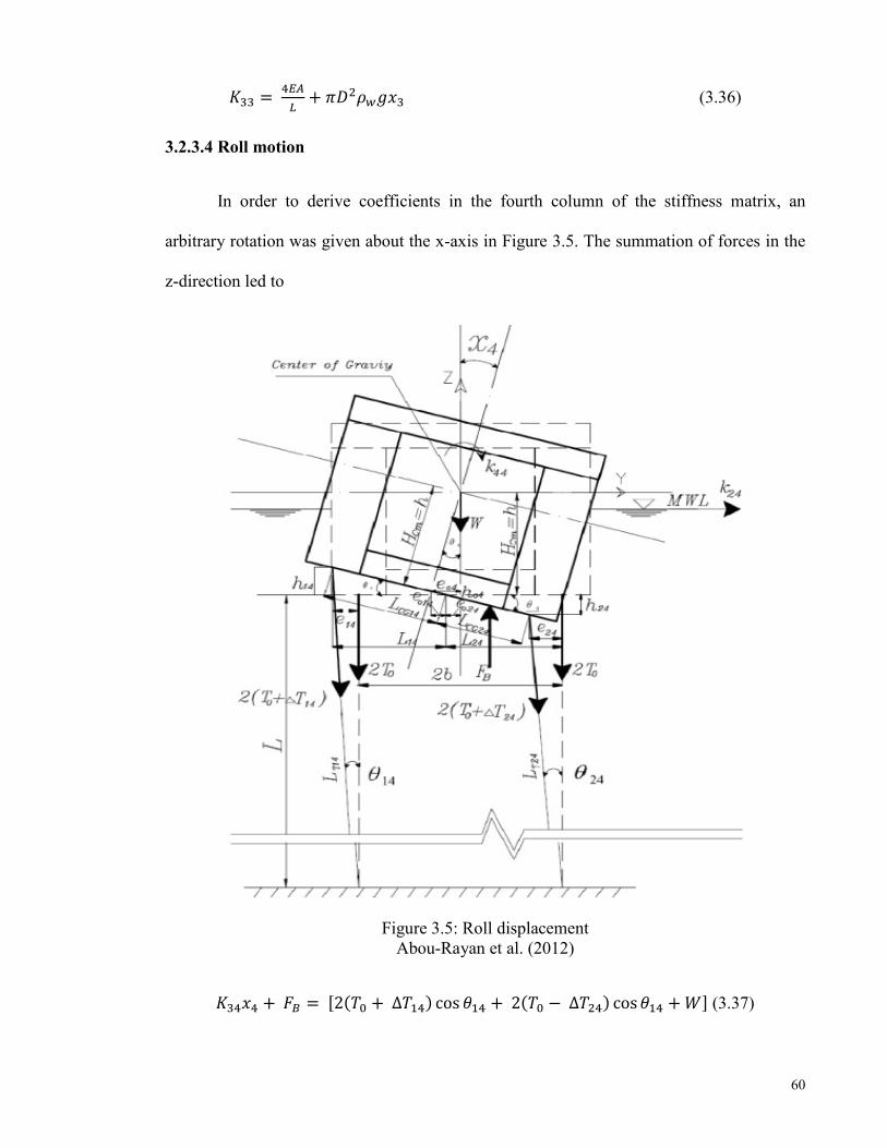
60
��� = ���
�+ �� ��� ��� (3.36)
3.2.3.4 Roll motion
In order to derive coefficients in the fourth column of the stiffness matrix, an
arbitrary rotation was given about the x-axis in Figure 3.5. The summation of forces in the
z-direction led to
Figure 3.5: Roll displacement Abou-Rayan et al. (2012)
����� + �� = [2(�� + ∆���) cos ��� + 2(�� − ∆���) cos ��� + � ] (3.37)
61
Due to the symmetry, change in tension in the near and rear tendon legs were equal and
expressed as
∆��� = ∆��� = ��
��� (3.38)
��� =�
��(∆��� + ∆���) (3.39)
However, ��� = 0 for the TLP tendons that is symmetrically placed to each other as
observed in the case at hand.
Again, the moment of resultant forces about the x-axis in Figure 3.5 was formulated as:
��� = �� ∗ ��� + ⟨2(�� + ∆���) cos ��� ∗ (� + ���) − 2(�� + ∆���) cos ��� ∗
(� − ���)⟩∗ 1��
� (3.40)
3.2.3.5 Pitch motion
The coefficients of the fifth column for the stiffness matrix as a result of pitching
were derived by giving an arbitrary moment about the y-axis in Figure 3.6.

62
Figure 3.6: Pitch displacement Abou-Rayan et al. (2012)
The equilibrium of forces in the heave direction yielded
��� = ⟨2(�� + ∆���) + 2(�� + ∆���) − 4��⟩∗ 1��
� (3.41)
Due to symmetry, ��� = 0
Again, by taking the moment of resultant forces about the x-axis in Figure 3.6,
��� = �� ∗ ��� + ⟨2(�� + ∆���) cos ��� ∗ (� + ���) − 2(�� + ∆���) cos ��� ∗
(� − ���)⟩∗ 1��
� (3.42)

63
3.2.3.6 Yaw motion
Finally, elements of the sixth column of the master stiffness matrix occurs when the TLP
was rotated about the z-axis as in Figure 3.7, the stiffness coefficients were obtained by
taking the summation of moment about the z-axis to be
Figure 3.7: Yaw displacement Abou-Rayan et al. (2012)
��� = 4(�� + ∆��) ∗ (�� + ��)/[�� + ��� (�� + ��)]�.� (3.43)
∆�� is the change in tendon tension force as a result of yaw rotation and this was given as:
∆�� = ��
�([�� + ��
� (�� + ��)]�.� − �) (3.44)
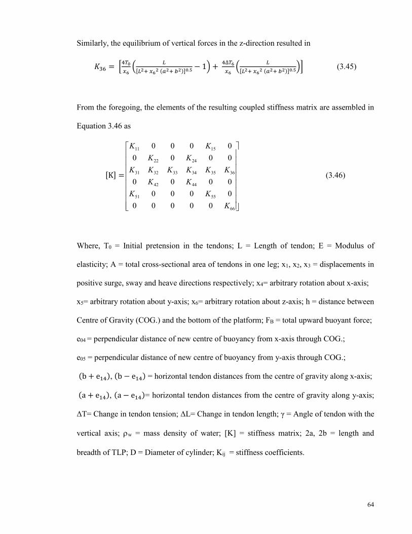
64
Similarly, the equilibrium of vertical forces in the z-direction resulted in
��� = ����
���
�
[��� ��� (��� ��)]�.� − 1� +
�∆��
���
�
[��� ��� (��� ��)]�.��� (3.45)
From the foregoing, the elements of the resulting coupled stiffness matrix are assembled in
Equation 3.46 as
[K] =
66
5551
4442
363534333231
2422
1511
00000
0000
0000
0000
0000
K
KK
KK
KKKKKK
KK
KK
(3.46)
Where, T0 = Initial pretension in the tendons; L = Length of tendon; E = Modulus of
elasticity; A = total cross-sectional area of tendons in one leg; x1, x2, x3 = displacements in
positive surge, sway and heave directions respectively; x4= arbitrary rotation about x-axis;
x5= arbitrary rotation about y-axis; x6= arbitrary rotation about z-axis; h = distance between
Centre of Gravity (COG.) and the bottom of the platform; FB = total upward buoyant force;
e04 = perpendicular distance of new centre of buoyancy from x-axis through COG.;
e05 = perpendicular distance of new centre of buoyancy from y-axis through COG.;
(b + e��), (b − e��) = horizontal tendon distances from the centre of gravity along x-axis;
(a + e��), (a − e��)= horizontal tendon distances from the centre of gravity along y-axis;
ΔT= Change in tendon tension; ΔL= Change in tendon length; γ = Angle of tendon with the
vertical axis; w = mass density of water; [K] = stiffness matrix; 2a, 2b = length and
breadth of TLP; D = Diameter of cylinder; Kij = stiffness coefficients.
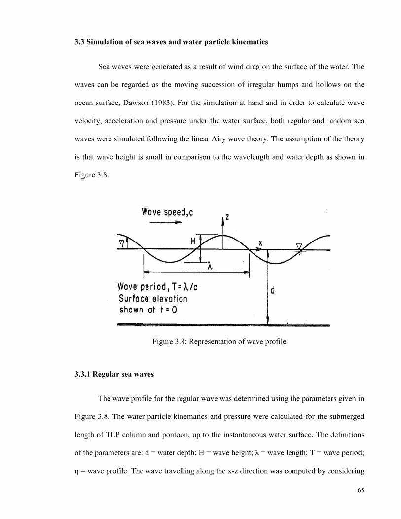
65
3.3 Simulation of sea waves and water particle kinematics
Sea waves were generated as a result of wind drag on the surface of the water. The
waves can be regarded as the moving succession of irregular humps and hollows on the
ocean surface, Dawson (1983). For the simulation at hand and in order to calculate wave
velocity, acceleration and pressure under the water surface, both regular and random sea
waves were simulated following the linear Airy wave theory. The assumption of the theory
is that wave height is small in comparison to the wavelength and water depth as shown in
Figure 3.8.
Figure 3.8: Representation of wave profile
3.3.1 Regular sea waves
The wave profile for the regular wave was determined using the parameters given in
Figure 3.8. The water particle kinematics and pressure were calculated for the submerged
length of TLP column and pontoon, up to the instantaneous water surface. The definitions
of the parameters are: d = water depth; H = wave height; λ = wave length; T = wave period;
η = wave profile. The wave travelling along the x-z direction was computed by considering

66
the governing equation for velocity potential with their respective boundary conditions as
found in standard texts such as Dawson (1983) and Chakrabarti (2005).
The wave profile equation was given in Equation 3.47 as:
η(x, z, t) = �
� cos Θ (3.47)
Where
Θ = k (� cos � + �sin �) – �t (3.48)
Θ is the wave phase; and β is the direction of propagation measured from the positive x-
axis.
� = � �
� is the wave number (3.49)
� = � �
� is the wave circular frequency (3.50)
The relationship between wave period and wavelength was given by the dispersion
equation as
�� = �����ℎ �� (3.51)
By differentiating the wave profile equation with respect to ‘x’ and ‘z’ coordinates, the
accompanying horizontal and vertical velocities from the motion were calculated and stated
in Equations 3.52 and 3.53 as
� = ��
� ������
���� �� cos (�� − ��) (3.52)
� = ��
�
���� ��
������ sin (�� − ��) (3.53)
The water particle accelerations were calculated by differentiating velocities with respect to
time and written in Equations 3.54 and 3.55 as:
�� = � ��
� ������
������ sin (�� − ��) (3.54)
�� = − � ��
�
���� ��
������ cos (�� − ��) (3.55)

67
The dynamic pressure for the linear wave theory was given as
P = ρg �
�
���� ��
���� �� cos(kx − ω t) + ρg (d − z) (3.56)
3.3.2 Random sea waves
A more realistic ocean environment was modelled by summing the individual wave
components of different directions, frequencies, phases and amplitudes altogether. Here,
ocean surface was assumed to be a random field that is stationary in time, homogeneous in
space and ergodic in nature. Since wave generates free surface motion, superposition of the
regular waves with Gaussian random variable was used to create random waves. The
random waves were simulated as unidirectional and directional sea waves.
3.3.2.1 Unidirectional and directional sea waves
The wave profile for unidirectional and directional sea waves were stated in
Equations 3.57 and 3.59 to be
�(�, �) = ∑ ��cos(��� − � ��+ ∅�)��� � (3.57)
�� = �2 ���(� �)∆� � (3.58)
�(�, �, �) = ∑ ��cos[��(� cos �� + � sin �� ) − � ��+ ∅�]��� � (3.59)
�� = �2���(� �)� (� , �)∆� �∆�� (3.60)
Where N is the number of wave components; �� is the amplitude of the ith wave
component; �� is wave number of the ith wave component; x is the x-coordinate of the point
along the wave direction. The ∅� represent the phase angle for the individual wave, which
are random variables in nature and uniformly distributed between (0, 2π). Furthermore,
Equation 3.57 was differentiated with respect to x and z and this led to the estimation of the
horizontal and vertical water velocities in Equations 3.61 and 3.62 respectively. Further
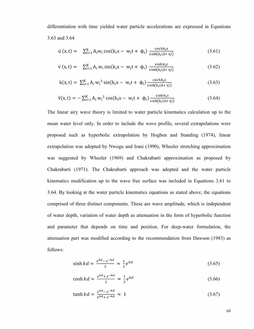
68
differentiation with time yielded water particle accelerations are expressed in Equations
3.63 and 3.64
u (x, t) = ∑ A�w���� � cos(k�x − w�t + ϕ �)
�������
�������(�� �)� (3.61)
v (x, t) = ∑ A���� � w� sin(k�x − w�t + ϕ �)
�������
�������(�� �)� (3.62)
u(x, t) = ∑ A���� � w�
� sin(k�x − w�t + ϕ �)�������
�������(�� �)� (3.63)
v(x, t) = − ∑ A���� � w�
� cos(k�x − w�t + ϕ �)���� ���
�������(�� �)� (3.64)
The linear airy wave theory is limited to water particle kinematics calculation up to the
mean water level only. In order to include the wave profile, several extrapolations were
proposed such as hyperbolic extrapolation by Hogben and Standing (1974), linear
extrapolation was adopted by Nwogu and Irani (1990), Wheeler stretching approximation
was suggested by Wheeler (1969) and Chakrabarti approximation as proposed by
Chakrabarti (1971). The Chakrabarti approach was adopted and the water particle
kinematics modification up to the wave free surface was included in Equations 3.61 to
3.64. By looking at the water particle kinematics equations as stated above, the equations
comprised of three distinct components. These are wave amplitude, which is independent
of water depth, variation of water depth as attenuation in the form of hyperbolic function
and parameter that depends on time and position. For deep-water formulation, the
attenuation part was modified according to the recommendation from Dawson (1983) as
follows:
sinh �� = ��� � �� ��
� ≈
�
���� (3.65)
cosh �� = ��� � �� ��
� ≈
�
���� (3.66)
tanh �� = ��� � �� ��
��� � �� �� ≈ 1 (3.67)

69
The dispersion relation for the deep-water case was simplified and given as
� � = �� (3.68)
This can also be formulated in terms of wavelength and wave period as follows
� = �
�� �� (3.69)
As earlier reported, random wave was simulated as the summation of different
regular wave components. The contribution of each component was accounted for via the
wave spectrum. Quite a number of empirical wave spectra that were simulated from the
collected data over time and for a particular place are available. Some of the wave spectra
include the Pierson Moskowitz (PM) spectrum, the Joint North Sea Wave Project
(JONSWAP), the TMA spectrum, the Bretschneider spectrum, the Torsethaugen spectrum
and the Ochi-Hubble spectrum among many others. A modified Pierson-Moskowitz (PM)
spectrum which was formulated based on significant wave height and angular peak
frequency was adopted from Veritas (2007) and represented in Equation 3.70 as
S��(w) = �
�� .H�
�w��.w������−
�
��
�
���
��
� (3.70)
Where
S��(w) is the Pierson Moskowitz (PM) spectrum; H� is the significant wave height; w� is
the angular peak frequency. With the known wave spectrum, the linear wave theory and the
wave height, synthetic sea state was simulated using random phase method, Chakrabarti
(1987). The algorithm for Monte Carlo simulation of individual wave frequencies and their
bandwidths were simulated from the Borgman (1967) and Goda (1970). A similar approach
was adopted by Ahmad (1996) and, Chandrasekaran and Jain (2002b) respectively. The
individual component frequencies ��, � �, � �, … � � are required to be non-correlating so

70
that they will not constitute harmonics. The selection of frequency was achieved in
FORTRAN by dividing the range of frequency from the lowest, � ��� to the highest, ����
into (N-1) sub-ranges with the dividing frequencies constituting a power series of
� �� = � ��� + � ��� � � ���
� �� (3.71)
� �� = ��� × �� … , (3.72)
� �� = � ���� × �� (3.73)
� � ��� = � �� × �� � � � (3.74)
Where
�� = �� ���
� ���
�(� ��)�
(3.75)
This was followed with the secondary dividing frequencies � ���, � ��
�,
� ���, … � ��
� �� that were chosen at random from the respective sub-ranges. The initial
frequency � ��� was set equal to � ��� and the last was as � � �� = ���� . The selection was
done with the aid of random number generation. The component frequency, w� and its
band width ∆w� were calculated for i = 1, 2, 3…... N as
� � = �
� (� ��
��� + � ���) (3.76)
∆� � = � ��� − � ��
��� (3.77)
The random process for the wave component frequency described above was
repeated for each run of the wave spectrum. The phase angle for each wave was achieved
with the help of the in-built random number in the FORTRAN software in the range of (0,
2π) so that the wave profile function would follow the Gaussian distribution. The number
of component waves, length of time step and duration of wave record were controlled so as
to realize an ocean environment that has characteristics of the real sea state. The length of
time step for the simulation of the wave profile equation and the numerical Newmark-Beta

71
equation was controlled so that the time interval satisfied the condition of ∆t ≤ 15f���
� .
The value of 0.2 seconds, which was smaller than the required was used as time step for the
simulation. The duration of the simulated wave record was 5000 seconds and 25000 data
points were generated in one run for the random waves.
From the uni-directional wave spectrum, cosine power-type energy spreading
function of directional short-crested wave spectra was expressed according to Veritas
(2007) as
�(� , �) = �(� ) � (�, � ) = �(� ) � (�) (3.78)
Where � (�, � ), and � (�) are directionality functions, � is the angle between the direction
of elementary wave trains and the main wave direction of the short-crested wave system.
The directional function, � (� , �) for wind sea in Equation 3.78 was simulated with the
frequency-dependence neglected and the approximation of D(W , θ) = D(θ). The
directional function used in this study was also employed in Sannasiraj et al. (1995) as
given below
� (�) = ���� � �� �
√��(� �⁄ � � �⁄ ) cos� �� − ��� (3.79)
Γ is the Gamma function and �� − �� ≤ �
�� (3.80)
� (�) is the directional function; �� as the main wave direction, and ‘n’ is a constant
ranging between n = 2 to n = 4 for wind sea. Veritas (2007)
3.4 Modified Morison wave force
A modified Morison equation that was based on strip method was employed to
calculate the wave force on the submerged portion of the TLP. Figure 3.9 shows the
regions where the Morison formula is applicable and the ISSC TLP lies in region III of the
small drag and large inertia. From the calculation of diffraction parameter and, the ratio of
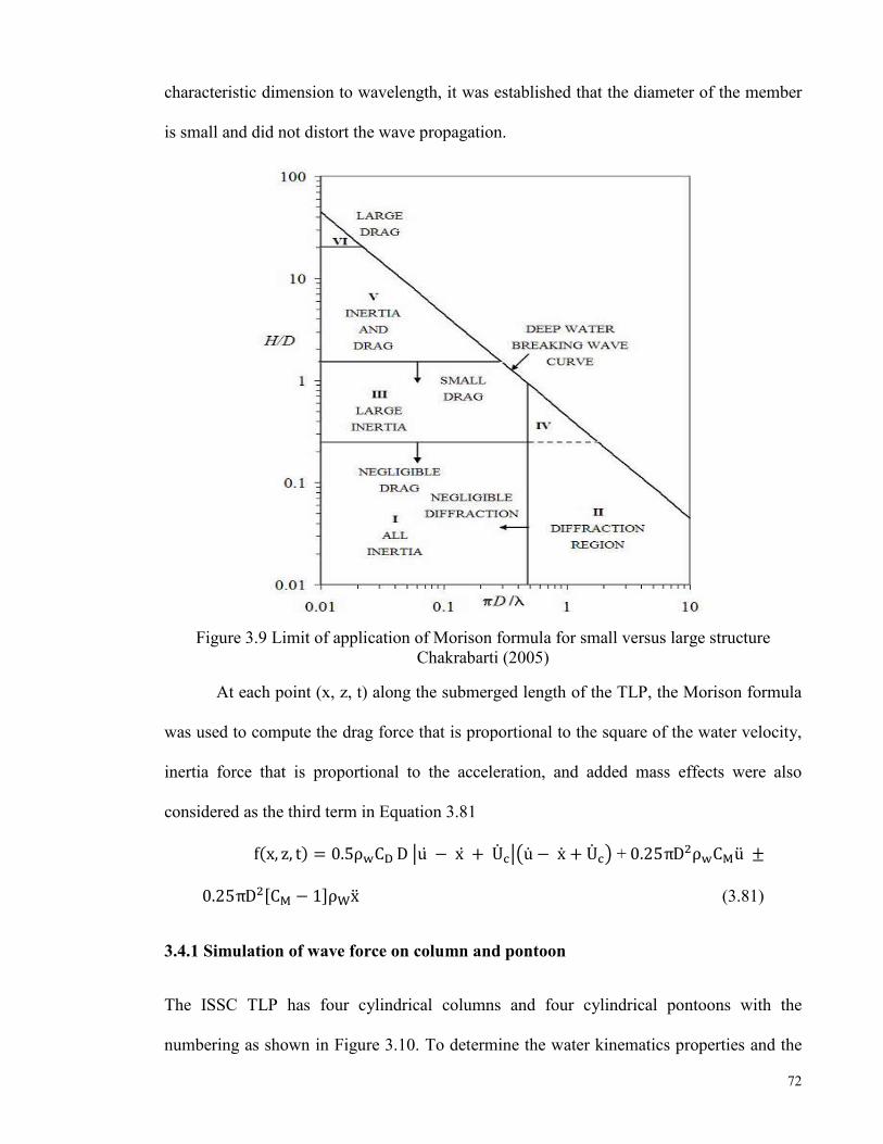
72
characteristic dimension to wavelength, it was established that the diameter of the member
is small and did not distort the wave propagation.
Figure 3.9 Limit of application of Morison formula for small versus large structure Chakrabarti (2005)
At each point (x, z, t) along the submerged length of the TLP, the Morison formula
was used to compute the drag force that is proportional to the square of the water velocity,
inertia force that is proportional to the acceleration, and added mass effects were also
considered as the third term in Equation 3.81
f(x, z, t) = 0.5ρ�C� D �u − x + U���u − x + U�� + 0.25πD�ρ�C�u ±
0.25πD�[C� − 1]ρ� x (3.81)
3.4.1 Simulation of wave force on column and pontoon
The ISSC TLP has four cylindrical columns and four cylindrical pontoons with the
numbering as shown in Figure 3.10. To determine the water kinematics properties and the

73
hydrodynamic forces on these members, a 6 points coefficient Gauss-Legendre of
numerical integration was programmed in FORTRAN and employed as
� = 0.5 ∗ (�1 + �1) + 0.5 ∗ (�1 − �1) ∗ � (3.82)
Where ‘a1’ and ‘b1’ are the lower and upper limit of integration as shown in Figure 3.10.
Equation 3.82 is in accordance with Chapra and Canale (2012) for determining integral.
Figure 3.10: Sketch of TLP plan and elevation
For arbitrarily oriented cylinder, the angle of orientation needs to be specified. The
orientation of the vertical column members is defined by ‘phi’ and ‘theta’ in the
FORTRAN program to be zero. For horizontal members 2 and 6, phi is 900 and theta is 00
while members 4 and 8 have phi as 900 and theta as –900 respectively.
The water motion produces horizontal and vertical velocities; and accelerations
along the x- and y-direction. The magnitude of the water velocity which is normal to the
cylinder axis is given in Equation 3.83 in accordance with Dawson (1983)
� = ��� + �� − ���� + �����
��
��
(3.83)
The velocity components along the x, y and z directions are

74
�� = � − ������ + ����
�� = � − ������ + ����
�� = − ������ + ���� (3.84)
Where
�� = sin �ℎ��cos �ℎ���;
�� = cos �ℎ��;
�� = sin �ℎ��sin �ℎ��� (3.85)
The values of water acceleration in the x, y and z directions are as given below
��� = �� − ������� + �����
��� = �� − ������� + �����
��� = − ������� + ����� (3.86)
From the water kinematics calculated above, the force per unit of cylinder length in the x, y
and z directions are given by general Morison equation as
�� = 1
2��� ���� + ���
�� �
4���
�� = 1
2��� ���� + ���
�� �
4���
�� = �
���� ���� + ���
�� �
���� (3.87)
The total force along the x, y and z directions were calculated by numerical integration with
the limits covering the entire area where the hydrodynamic force acts as
�� = ∫ ����
����; �� = ∫ ��
��
����;
�� = ∫ ����
���� ; � � = ∫ � ∗ ��
��
����;
� � = ∫ � ∗ ����
����; � � = ∫ � ∗ ��
��
���� (3.88)

75
Due to the limited experimental data, drag and inertia coefficient constants were chosen
from the range of (0.6 to 1.0) for drag and (1.5 to 2.0) for inertia as recommended by the
American Petroleum Institute.
3.4.2 Total wave and current induced forces
Finally, the total force and moment on each column and pontoon along the six degrees of
freedom were added together. The wave force was further simplified into surge, sway and
heave components as stated in Equations 3.89 – 3.94.
Surge Force = F� = �∑ �F� �(k) + F��
(k)���� � �
������cos α + �F��
+ F���
������� (3.89)
Sway Force = F� = �∑ �F� �(k) + F��
(k)���� � �
������sin α + �F��
+ F���
������� (3.90)
Heave Force = F� = [F� ]������ + �F��+ F��
��������
(3.91)
The total force in the x, y and z directions are FX, FY, and FZ respectively. The
parameter
n
k 1
is the summation over the vertical column; k is the number of columns; is
the angle of wave incidence; FD (k) and FI (k) are total drag and inertia forces on kth
column; Fd and Fi are the total drag and inertia force on the pontoon; Fv is the total vertical
hydrodynamic pressure force on the column bottom; and subscripts x, y and z represent the
directions respectively.
Drag and inertia loadings on pontoon and vertical column members also caused moment
about the x, y and z-axes which were known as roll, pitch and yaw moments respectively.
These moments about the x, y and z- axes were obtained by multiplying the above-
mentioned forces with their respective lever arms and with respect to their axes of rotations
as follows:

76
M� = [∑ {M� (k) + M�(k)}��� � ]������ sin α + �M��
+ M���
����+ �M��
�������
(3.92)
M� = [∑ {M� (k) + M�(k)}��� � ]������ cos α + �M��
+ M���
����+ �M��
�������
(3.93)
M� = ∑ [F� (k) + F�(k) ] y���� � (3.94)
3.4.3 Current force
The parameter U� in the first component of Equation 3.81 is the wind-drift current
velocity. This was modelled with linear profile in the form of Equation 3.95 and taken to be
steady, horizontal and linearly varying with the water depth as
U�,���� = U�,����(0) ��
�� (3.95)
Where
U� is the current velocity at the level z, z ≤ 0; z is the distance from the Still Water Level
(SWL) and positive upwards; U�,����(0) is the tidal current velocity at the SWL; d is the
water depth to the SWL.
3.4.4 Wind forces
The superstructure of the tension leg platform, which lies above the still water line, is
open to the wind forces, also known as aerodynamic forces. The wind forces on the TLP
are primarily governed by the local wind speed for the TLP location. This is calculated by
using simplified approach where the force is made proportional to the square of the relative
velocity through the use of the slope coefficients. However, for the computation of wind
force per unit area acting above the still water line part of the TLP, wind speed profile, the
Simiu and Leigh wind spectrum and American Petroleum Institute (API) spectrum were
77
used in FORTRAN coding and Abaqus/Aqua module respectively. The overall wind load
on the platform is given in Equation 3.96 as
�� (�) = 0.5���������(�) + ����(�) − �(�)�
� (3.96)
Where,
a = Mass density of the air, �� is the wind drag coefficient, �� is the projected area along
the wind direction, ��(�) is the mean wind speed, ����(�) is the fluctuating wind
component, � is the structural velocity.
In Equation 3.96, it was assumed that the directions of the mean wind and wave force on
the platform surge motion coincide with each other.
The wind speed u (y, z, t) may be expressed as the summation of mean and
fluctuating part of the wind as written in Equation 3.97:
),,()(),,( tzyuzutzyu (3.97)
Where
)(zu is the mean wind speed; and ),,( tzyu is the fluctuating wind velocity. These two
components were evaluated in the manner discussed below.
3.4.4.1 Mean wind speed
The wind speed above the sea surface varies with time and height. In order to
estimate the value of wind speed at the height ‘z’, the mean wind speed at the reference
height together with the logarithmic wind speed profile from Veritas (2007), and Simiu and
Leigh (1984) was used in Equation 3.98 as
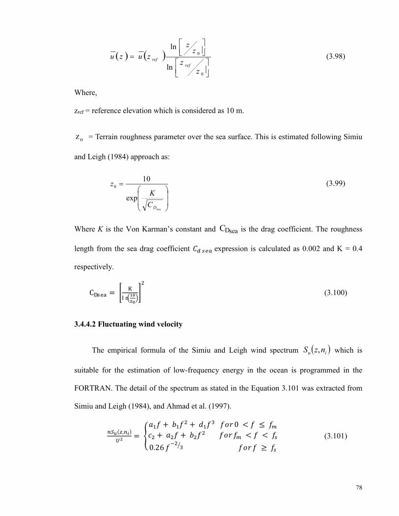
78
0
0
ln
ln
zz
zz
zuzuref
ref (3.98)
Where,
zref = reference elevation which is considered as 10 m.
oz = Terrain roughness parameter over the sea surface. This is estimated following Simiu
and Leigh (1984) approach as:
seaDC
Kz
exp
100
(3.99)
Where K is the Von Karman’s constant and seaDC is the drag coefficient. The roughness
length from the sea drag coefficient �� ��� expression is calculated as 0.002 and K = 0.4
respectively.
C���� = ��
�����
����
�
(3.100)
3.4.4.2 Fluctuating wind velocity
The empirical formula of the Simiu and Leigh wind spectrum iu nzS , which is
suitable for the estimation of low-frequency energy in the ocean is programmed in the
FORTRAN. The detail of the spectrum as stated in the Equation 3.101 was extracted from
Simiu and Leigh (1984), and Ahmad et al. (1997).
��� (�,��)
� � = �
��� + ���� + ���� ��� 0 < � ≤ ��
�� + ��� + ���� ��� �� < � < ��
0.26 ���
�� ��� � ≥ ��
(3.101)
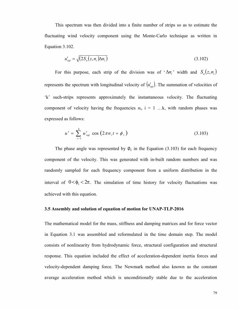
79
This spectrum was then divided into a finite number of strips so as to estimate the
fluctuating wind velocity component using the Monte-Carlo technique as written in
Equation 3.102.
iiueqi nnzSu ,2 (3.102)
For this purpose, each strip of the division was of ‘ in ’ width and iu nzS ,
represents the spectrum with longitudinal velocity of eqiu . The summation of velocities of
‘k’ such-strips represents approximately the instantaneous velocity. The fluctuating
component of velocity having the frequencies ni, i = 1 …k, with random phases was
expressed as follows:
ii
k
ieqi tnuu
2cos1
(3.103)
The phase angle was represented by ∅� in the Equation (3.103) for each frequency
component of the velocity. This was generated with in-built random numbers and was
randomly sampled for each frequency component from a uniform distribution in the
interval of 20 i . The simulation of time history for velocity fluctuations was
achieved with this equation.
3.5 Assembly and solution of equation of motion for UNAP-TLP-2016
The mathematical model for the mass, stiffness and damping matrices and for force vector
in Equation 3.1 was assembled and reformulated in the time domain step. The model
consists of nonlinearity from hydrodynamic force, structural configuration and structural
response. This equation included the effect of acceleration-dependent inertia forces and
velocity-dependent damping force. The Newmark method also known as the constant
average acceleration method which is unconditionally stable due to the acceleration

80
assumptions and iteration in each time step, is adopted for the solution of the problem. The
dynamic equation for the next time step is shown in Equation 3.104.
MU�� �� + CU���� + KU���� = �� �t, U, U������
(3.104)
The method was founded on the assumptions that acceleration varies in each time step as:
U���� = U� + �(1 − δ)U� + δU�����Δt (3.105)
U���� = U� + U�Δt + ���
�− α� U� + αU�����Δt� (3.106)
To determine the displacement at the next time step, U����, U�� �� is solved in terms of
U���� and substituted into Equation 3.105. This yields expression for U�� �� and � ���� in
terms of U����. These terms were then substituted into Equation 3.104 for the computation
of U����. The value was substituted into Equation 3.105 and 3.106 to calculate U�� ��
and U����. The second ordinary differential equation of Equation 3.104 is nonlinear,
changes at every time step and also the variation in tendon tension makes the TLP
response-dependent in nature.
In order to cater for these changes, a stable and accurate numerical method is
essential. The Newmark-beta integration method was adopted due to the inherent
parameters (α and δ) in the method that control the accuracy and stability. The algorithm
for the numerical method from Bathe (1982) was programmed in the following sequence
inside the FORTRAN as follows:
1. Formulation of stiffness matrix ‘K’, mass matrix ‘M’ and damping matrix ‘C’
2. Initialize values for U, � , �
3. Assign values to time step ∆ � and to parameters α and δ. This was followed with
computation of the following integration constants:
δ ≥ 0.5 α ≥ 0.25(δ + 0.5)� ;
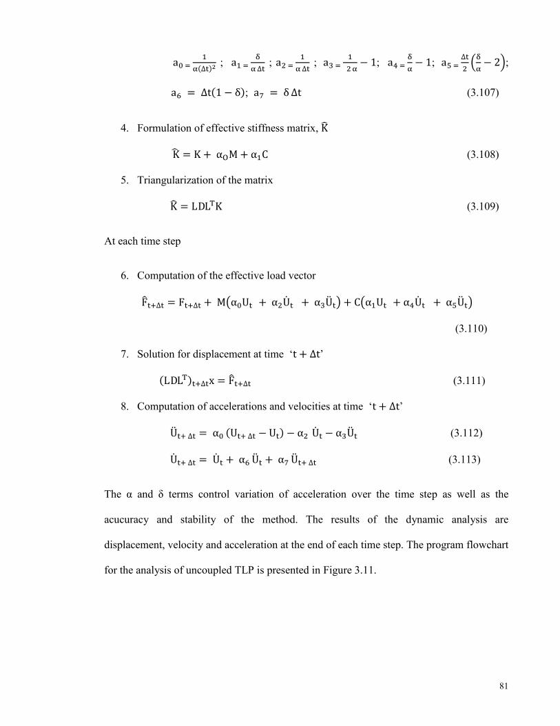
81
a� ��
�(∆�)� ; a� �
�
� ∆� ; a� �
�
� ∆� ; a� �
�
� �− 1; a� �
�
�− 1; a� �
∆�
��
�
�− 2�;
a� = ∆t(1 − δ); a� = δ∆t (3.107)
4. Formulation of effective stiffness matrix, K�
K� = K + α� M + α�C (3.108)
5. Triangularization of the matrix
K� = LDL�K (3.109)
At each time step
6. Computation of the effective load vector
F���∆� = F��∆� + M�α�U� + α�U� + α�U�� + C�α�U� + α�U� + α�U��
(3.110)
7. Solution for displacement at time ‘t + ∆t’
(LDL�)��∆�x = F���∆� (3.111)
8. Computation of accelerations and velocities at time ‘t + ∆t’
U�� ∆� = α� (U�� ∆� − U�) − α� U� − α�U� (3.112)
U�� ∆� = U� + α� U� + α� U�� ∆� (3.113)
The α and δ terms control variation of acceleration over the time step as well as the
acucuracy and stability of the method. The results of the dynamic analysis are
displacement, velocity and acceleration at the end of each time step. The program flowchart
for the analysis of uncoupled TLP is presented in Figure 3.11.
82
Figure 3.11: Flowchart for Uncoupled Nonlinear Analysis Program (UNAP-TLP-2016)
3.6 Simulation of CNAP-TLP-2016 in Abaqus Software
Unlike the stiffness approach in an uncoupled model, Abaqus finite element tool
modelled the platform and tendons together with proper couplings among the various
modes of degree of freedoms. With this approach, derivation of stiffness coefficients was
achieved without resulting in reaction of forces as previously adopted by other authors and
for uncoupled model in this present study. The general-purpose finite element tool was

83
used to discretize the platform as shown in Figure 3.12. The model geometry of Figure 4.12
consists of 84 nodes and 80 elements for all the tendons, while platform column and
pontoon is made up of 86 nodes and 87 elements in 450 metres water depth for ISSC TLP.
The fluid flow environment is modelled using the empirical formulas of the linear
wave theory and the Morison formula while the platform and mooring lines are represented
with the aid of finite element formulation in the Abaqus environment. The Abaqus/Aqua
analysis module of the Abaqus software is specifically designed to apply current, wave and
wind loading to submerged structures such as marine risers and offshore pipelines
installation, Dassault (2009). The module is not an alternative option for hydrodynamic
software for offshore problems but rather, this thesis used general purpose finite element
software for the solution of nonlinear dynamic analysis of the TLP.
Figure 3.12: Finite element discretization of model geometry
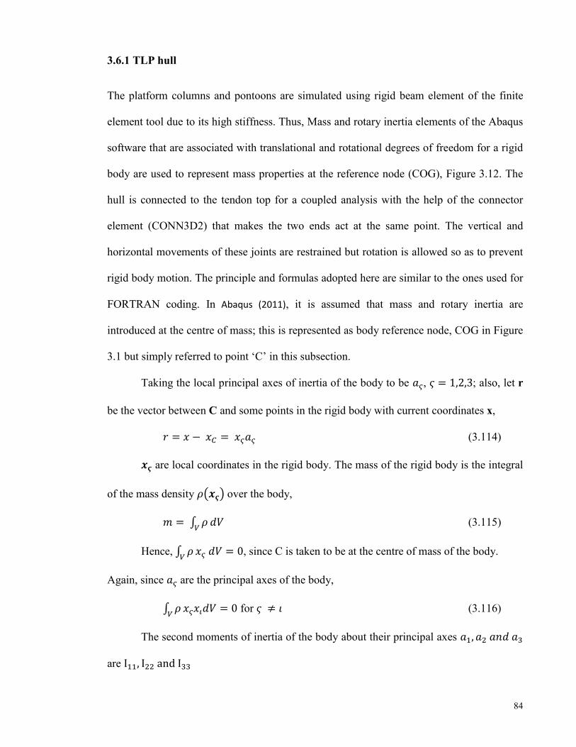
84
3.6.1 TLP hull
The platform columns and pontoons are simulated using rigid beam element of the finite
element tool due to its high stiffness. Thus, Mass and rotary inertia elements of the Abaqus
software that are associated with translational and rotational degrees of freedom for a rigid
body are used to represent mass properties at the reference node (COG), Figure 3.12. The
hull is connected to the tendon top for a coupled analysis with the help of the connector
element (CONN3D2) that makes the two ends act at the same point. The vertical and
horizontal movements of these joints are restrained but rotation is allowed so as to prevent
rigid body motion. The principle and formulas adopted here are similar to the ones used for
FORTRAN coding. In Abaqus (2011), it is assumed that mass and rotary inertia are
introduced at the centre of mass; this is represented as body reference node, COG in Figure
3.1 but simply referred to point ‘C’ in this subsection.
Taking the local principal axes of inertia of the body to be ��, � = 1,2,3; also, let r
be the vector between C and some points in the rigid body with current coordinates x,
� = � − �� = ���� (3.114)
�� are local coordinates in the rigid body. The mass of the rigid body is the integral
of the mass density ����� over the body,
� = ∫ ��
�� (3.115)
Hence, ∫ ��
�� �� = 0, since C is taken to be at the centre of mass of the body.
Again, since �� are the principal axes of the body,
∫ ��
������ = 0 for � ≠ � (3.116)
The second moments of inertia of the body about their principal axes ��, �� ��� ��
are I��, I�� and I��

85
I�� = ∫ ρ�
((x�)� + (x�)�)dV (3.117)
I�� = ∫ ρ�
((x�)� + (x�)�)dV (3.118)
I�� = ∫ ρ�
((x�)� + (x�)�)dV (3.119)
The rotary inertia tensor is computed and written using this notation
�= ∑ ������ � ���� (3.120)
The velocity of any point of the rigid body is stated as
u = u� + ω × r (3.121)
Where � = � is the angular velocity of the body. The acceleration of the body is
determined from the time derivate of Equation 3.121 as
u = u� + ω × r + ω × (ω × r) (3.122)
The equilibrium equations in a strong form represent the balance of linear
momentum and balance of angular momentum and these are given as follows:
m u�� = f (3.123)
I.ω + ω × I.ω = m� (3.124)
In the weak form, the equilibrium equation is
�� � + �� ��� = 0 (3.125)
The internal or d’Alembert force contribution is
δW � = − � ρ δ�
u.udV
= − m u�.δu� − (I.ω + ω × I.ω ).δθ (3.126)
Where δu = δu� + δθ × r is the variation of the position of a point in the body, ��� is the
variation of the position of the rigid body reference mode and �� is the variation of the
rotation of the rigid body reference node.
The external loading condition contribution is
86
δW ��� = f.δu� + m .δθ (3.127)
3.6.2 TLP tendons
Tendons are modelled with the help of finite beam elements. Although a beam
element is a line element, it has stiffness connected with the deformation line. The hybrid
beam element of the Timoshenko beam type is used for tendon modelling because of its
advantage over the usual finite element displacement method. Basically, for geometrically
nonlinear problems in which beams undergo large displacement and rigid in axial, hybrid
beam elements employ general formulation that considers axial, bending and transverse
shear forces in the elements, as well as nodal displacements and rotations. Timoshenko
beam is suitable for slender structures and also allows for transverse shear deformation.
The mass matrix formulation is based on consistent mass method. The orientation of the
beam cross-section is correctly chosen so as to define correct bending plane. The axis
system is local right-handed t, n1, n2, where ‘t’ is the tangent to the axis of the element,
positive from the first node to the second node of the element, n1 and n2 are local
directions of the cross-sections. Each node of the beam has six degrees of freedom active.
Hybrid beam elements of Abaqus which are suitable for slender situations and for which
the axial stiffness is very large compared to the bending stiffness are adopted. A solid
cross-section Timoshenko beam is adopted. The ISSC TLP case study that is considered
does not expressly provide the cross-section except the area. Nevertheless, the cross-section
and the dimensions are determined from the mass moment of inertia and existing TLPs.
The axial and bending behaviour of the beam according to Abaqus (2011)
can be expressed in the following manner:
The internal virtual work of the beam is stated as
δW �� = ∫ (Nδϵ+ M�δK� + M�δK� + M�δe�)
�dL (3.128)

87
This can be written in another form by introducing axial force variable, �� as
δW �� = ∫ �N�δε+ M�δK� + M�δK� + M�δe� + δλ(N − N�)�
�dL (3.129)
Here, �� is a Lagrange multiplier introduced to impose the constraint N = N�. A linear
combination of these expressions is
δW �� = ρδW �
� + (1 − ρ)δW �� (3.130)
δW �� = ∫ [(ρN + (1 − ρ)N�)δε+ M�δK� + M�δK� + M�δe� + (1 −
�
ρ)δλ(N − N�)] dL (3.131)
The contribution of this term to the Newton scheme is then stated as
∫ �
(ρdN + (1 − ρ)δN�)δε+ dM�δK� + dM�δK� + dM�δe� +
(1 − ρ)δλ(dN − dN�) +
N�dδε+ M�dδK� + M�dδK� + M�dδe�
��
dL
(3.132)
Where
N � = ρN + (1 − ρ)N� (3.133)
The tangent stiffness of the section behaviour yielded
�
dN�
dM�
dM�
dM�
� =
⎣⎢⎢⎡
A�� A�� A�� A��
A�� A�� A��
sym A�� A��
A��⎦⎥⎥⎤
�
dεdK�
dK�
de�
� (3.134)
ε is axial strain, K� K�are beam curvature, e� is the torsional strain, N= axial force, M� =
bending moment, M� = warping moment and M� is the twisting moment.
if ����� < ���, ��� (where L is the element length), then the beam is flexible axially and
the mixed formulation is unnecessary. Otherwise, the assumption is that an inverse of the
first equation above defines �� from ���:
dε = �
���(dN� − A��dK� − A��dK� – A��de�) (3.135)

88
Also
dM� = �A�� − ���
�
���� dK� + �A�� −
������
���� dK� + �A�� −
������
���� de� +
���
���dN� (3.136)
dM� = �A�� − ������
���� dK� + �A�� −
����
���� dK� + �A�� −
������
���� de� +
���
���dN�
(3.137)
dM� = �A�� − ������
���� dK� + �A�� −
������
���� dK� + �A�� −
����
���� de� +
���
���dN�
(3.138)
By multiplying first tangent section stiffness by � and the second is multiplied by (1 − �),
the Newton contribution of the element becomes
∫ ⌊δεδK�δK�δe�A��δλ⌋�
[A�]
⎩⎪⎨
⎪⎧
dεdK�
dK�
de�
dN� ⎭⎪⎬
⎪⎫
+ ∫ (N�dδε+ M�dδK� + M�dδK� +�
M�dδe�) dL (3.139)
= − ∫ �N�δε+ M�δK� + M�δK� + M�δe�
+ A��δλ(1 − ρ) ��� ��
����
��
dL (3.140)
Where [�] is
⎣⎢⎢⎢⎢⎢⎢⎢⎢⎢⎡���� ���� ���� ���� 1 − �
��� − (1 − �)���
�
���
��� − (1 − �)������
���
��� − (1 − �)������
���
(1 − �)���
���
��� − (1 − �)���
�
���
��� − (1 − �)������
���
(1 − �)���
���
���� ��� − (1 − �)���
�
���
(1 − �)���
���
− (1 − �)1
���⎦⎥⎥⎥⎥⎥⎥⎥⎥⎥⎤
(3.141)

89
The variable �� is taken as an independent value at each integration point in the element. �
as �
���� is chosen where � is a small value. With this choice and by ensuring the variables
�� are eliminated after the displacement variables of each element, the Gaussian elimination
has no difficulty in solving the equations.
3.6.3 Connector elements
In order to have an integrated TLP unit, the connector element is used to link
platform hull and tendons together. The advantage of using the connector element is due to
the fact that they do not eliminate degrees of freedom at the connection node but rather
imposed kinematic constraints with Lagrange multipliers. The CONN3D2 connector
element for 3-dimensional space and JOIN type of translational basic connection are used
in fixing the connecting nodes together. Therefore, kinematic constraints are u1 = u2 = u3 =
0. The rotational degrees of freedom are not fixed but free to rotate to prevent rigid mode.
3.6.4 Numerical solution for CNAP-TLP-2016
The problem at hand is all about finding a solution to the developed finite element model
and this can only be made possible by writing force and moment equilibrium equations at
all times for the entire body. The equation of motion was written internally by Abaqus
software using the virtual work principle and the finite element approximation of the
equilibrium equation in accordance with
M��u� + I� − P� = 0 (3.142)
Where, M�� = ∫ ρ���N �.N � dV� is the consistent mass matrix; I� = ∫ β�
��: σ d V� is
the internal force vector and P� = ∫ N ��
.t ds + ∫ N ��
.F dv as the external force vector.
The matrix and vector refer to matrices and vectors in the space of nodal variables uN.

90
The implicit integration method which is a generalization of the Newmark operator
is employed due to its control on numerical damping. This solves the dynamic problem at
time (t + Δt) based not only at the value ‘t’ but also on the same quantity at ‘t + Δt’. The in-
built automatic time step control based on half-increment residual is employed.
Equation 3.142 is replaced with a balance of D’Alembert forces at the end of the
time step and a weighted average of the static forces at the beginning and end of the time
step as follows:
M��u����� + (1 + α) �I����� − P����� � − α �I�� − P�� � +
L����� = 0 (3.143)
Where L����� is the sum of Lagrange multiplier forces associated with the degree of
freedom N. Equation 3.143 is then solved using the Newmark formula for displacement
and velocity integration
u���� = u� + Δtu� + Δt� ���
�− β� u� + βu���� � (3.144)
����� = �� + Δt �(1 − γ)u� + γu����� (3.145)
Where
� = �
�(1 − �)� ; � =
�
�− � ; −
�
� ≤ � ≤ 0 (3.146)
The whole procedure is achieved by writing an input text-file to capture every detail of the
platform following the flowchart in Figure 3.13 and a typical text file is included as
Appendix B in this report.
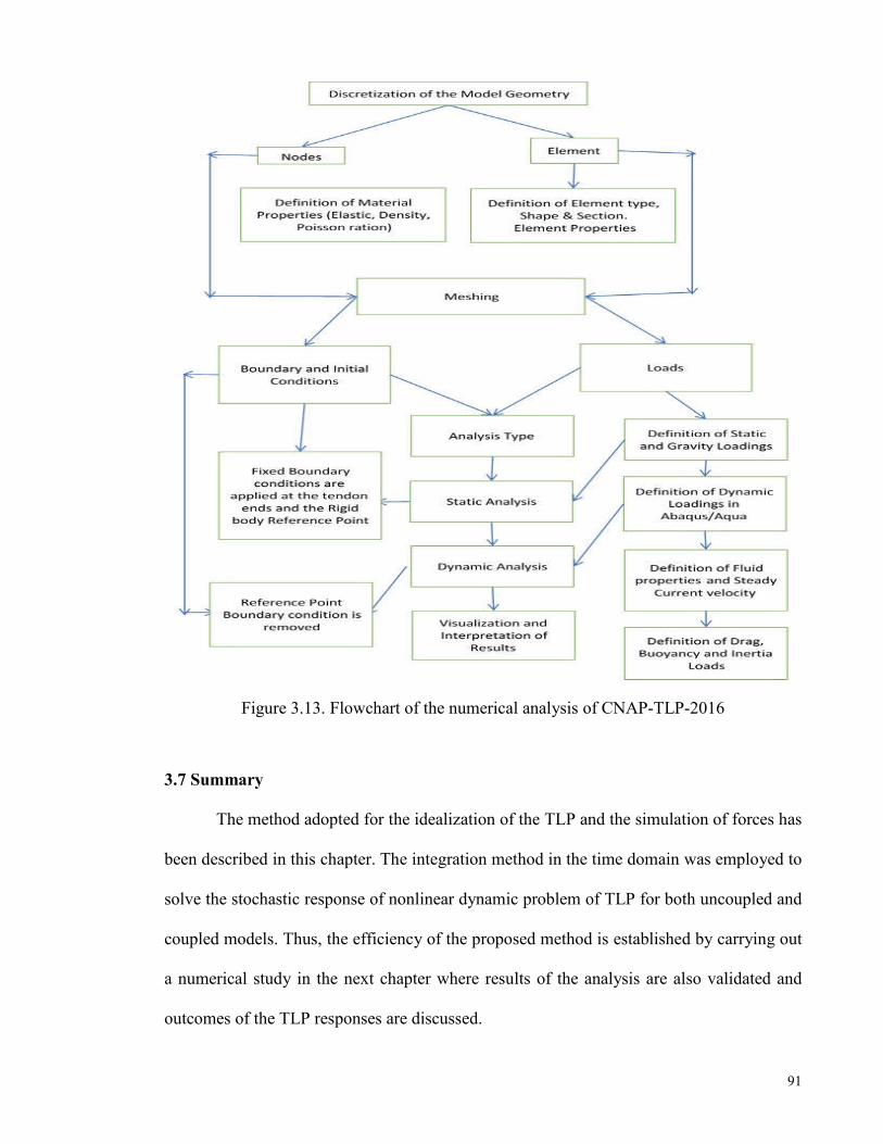
91
Figure 3.13. Flowchart of the numerical analysis of CNAP-TLP-2016
3.7 Summary
The method adopted for the idealization of the TLP and the simulation of forces has
been described in this chapter. The integration method in the time domain was employed to
solve the stochastic response of nonlinear dynamic problem of TLP for both uncoupled and
coupled models. Thus, the efficiency of the proposed method is established by carrying out
a numerical study in the next chapter where results of the analysis are also validated and
outcomes of the TLP responses are discussed.

92
CHAPTER 4: RESULTS AND DISCUSSION
4.1 Introduction
This chapter deals with the validation of the numerical model of Uncoupled
Nonlinear Analysis Program (UNAP-TLP-2016) simulated in FORTRAN program with the
published results so as to establish reliability of the proposed program. The proposed
program was then used to simulate various environmental conditions on an uncoupled TLP
model. The influence of current, wind and wave loads on the motion response in regular,
random and directional seas were also studied. The characterization of sea-wave
fundamentally governs the loads and responses of the TLP. This was proven by idealizing
the ocean surface as regular wave, random wave and directional random wave seas. The
real sea is probably not regular and representing it as one might not only be erroneous but
also undermine accurate assessment of forces and motions of the TLP. The nonlinear
analysis of the behaviour of the coupled TLP model was carried out in Abaqus software.
This was followed with validation of the obtained results with results of time-domain from
published works. The chapter concludes with various parametric studies on the effect of
different load combinations, TLP tendon dynamics, varying wave height and wave period
and vice-versa. The results and discussions are thus presented.
4.2 Validation of UNAP-TLP-2016 with published result
The outcomes of static and dynamic analysis obtained from the UNAP-TLP-2016 need to
be validated either with an experimental or similar time-domain program. Due to the
absence of an offshore experimental facility in our laboratory, the developed program was
validated with the previous work by Chitrapu and Ertekin (1992), Chitrapu and Ertekin
(1993), Chitrapu and Ertekin (1995); and Chitrapu, Ertekin, and Paulling (1993). The

93
platform characteristics and principal dimensions that was used for the comparison are
shown in Table 4.1 and Table 4.2 respectively. It should be noted that the platform
geometry and fundamental characteristics were the same in both models.
Table 4.1: Geometrical and mechanical characteristics of TLP Chitrapu and Ertekin (1992)
Number of Columns 4
Number of Pontoons 4 Tether diameter 0.40 m
Length of TLP hull 44.1 m
Diameter of Column 14.2 m
Water depth 500.0 m
Draft 26.6 m
COG above SWL 9.25 m
Displacement volume 33,400 m3
Table 4.2: Mechanical features of TLP, Ahmad (1996)
Total Tether Pretension 1.245×10⁸ N
Center to center spacing 58.3 m
Buoyancy force 3.34×10⁸ N
Mass of Platform 2.095×10⁷ kg
Axial Stiffness 5806 t/m
Weight of tether 5257 tons
Radii of Gyration (Rx, Ry, Rz) 29.15, 29.15 & 32.15 m
At the original equilibrium position of the TLP, the summation of vertical forces ensured
static equilibrium going by Equation 4.1
W + 4T − F� = 0 (4.1)
Where, W= total weight of the platform in the air; T= Initial Pretension in each tendon and
F�= total buoyancy force. The natural time periods of the TLP as reported by Ahmad
(1996) is given in Table 4.3 while Equation 4.2 was adopted to calculate the natural time
periods of the TLP for the present study, and this was found corresponding with the
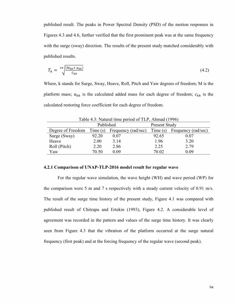
94
published result. The peaks in Power Spectral Density (PSD) of the motion responses in
Figures 4.3 and 4.6, further verified that the first prominent peak was at the same frequency
with the surge (sway) direction. The results of the present study matched considerably with
published results.
�� = �(���� ���)
���
�� (4.2)
Where, k stands for Surge, Sway, Heave, Roll, Pitch and Yaw degrees of freedom; M is the
platform mass; ��� is the calculated added mass for each degree of freedom; ��� is the
calculated restoring force coefficient for each degree of freedom.
Table 4.3: Natural time period of TLP, Ahmad (1996) Published Present Study Degree of Freedom Time (s) Frequency (rad/sec) Time (s) Frequency (rad/sec) Surge (Sway) 92.20 0.07 92.65 0.07 Heave 2.00 3.14 1.96 3.20 Roll (Pitch) 2.20 2.86 2.25 2.79 Yaw 70.50 0.09 70.02 0.09
4.2.1 Comparison of UNAP-TLP-2016 model result for regular wave
For the regular wave simulation, the wave height (WH) and wave period (WP) for
the comparison were 5 m and 7 s respectively with a steady current velocity of 0.91 m/s.
The result of the surge time history of the present study, Figure 4.1 was compared with
published result of Chitrapu and Ertekin (1993), Figure 4.2. A considerable level of
agreement was recorded in the pattern and values of the surge time history. It was clearly
seen from Figure 4.3 that the vibration of the platform occurred at the surge natural
frequency (first peak) and at the forcing frequency of the regular wave (second peak).
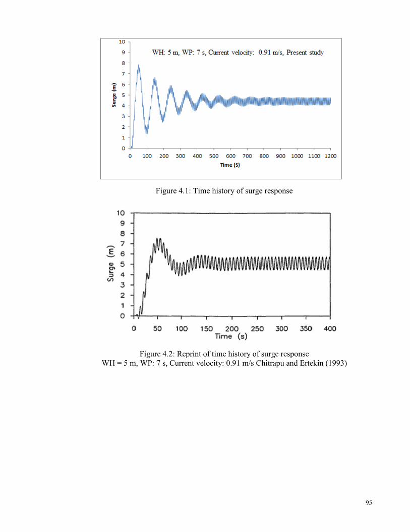
95
Figure 4.1: Time history of surge response
Figure 4.2: Reprint of time history of surge response
WH = 5 m, WP: 7 s, Current velocity: 0.91 m/s Chitrapu and Ertekin (1993)

96
Figure 4.3: PSD of surge response (Present study)
Further levels of similarities were observed for heave time histories in Figures 4.4
and 4.5 respectively with the close matching in the trend and values. Figure 4.6 presents the
heave PSD with the first prominent peak at surge natural period. By contrast, the second
peak was due to forcing frequency of the wave. The steady state was reached earlier in the
published result compared to the present study, this can be due to differences in numerical
algorithm assumptions. At the final run, both models had similar steady state forms in the
degrees of freedom. There is a widely-held view that the coupling due occur among the
degrees of freedom.

97
Figure 4.4: Time history of heave response
Figure 4.5: Reprint of time history of heave response
WH = 5 m, WP: 7 s, Current velocity: 0.91 m/s Chitrapu and Ertekin (1993)
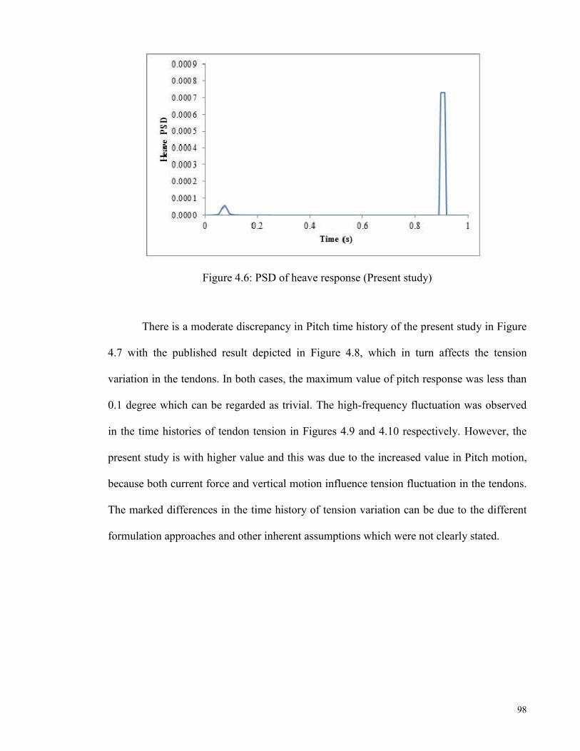
98
Figure 4.6: PSD of heave response (Present study)
There is a moderate discrepancy in Pitch time history of the present study in Figure
4.7 with the published result depicted in Figure 4.8, which in turn affects the tension
variation in the tendons. In both cases, the maximum value of pitch response was less than
0.1 degree which can be regarded as trivial. The high-frequency fluctuation was observed
in the time histories of tendon tension in Figures 4.9 and 4.10 respectively. However, the
present study is with higher value and this was due to the increased value in Pitch motion,
because both current force and vertical motion influence tension fluctuation in the tendons.
The marked differences in the time history of tension variation can be due to the different
formulation approaches and other inherent assumptions which were not clearly stated.

99
Figure 4.7 Time history of pitch response
Figure 4.8 Reprint of time history of pitch response WH = 5 m, WP: 7 s, Current velocity: 0.91 m/s Chitrapu and Ertekin (1993)

100
Figure 4.9 Time history of tension response
Figure 4.10 Reprint of time history of tension response WH: 5 m, WP: 7 s, Current velocity: 0.91 m/s Chitrapu and Ertekin (1993)
4.2.2 Validation of UNAP-TLP-2016 model result for random waves
The developed UNAP-TLP-2016 model program can handle regular waves and
random waves in both long and short crested seas. Since the model was later used to
simulate long and short crested seas, validation of the model was carried out for the

101
simulated random waves for the same platform characteristics. In Chitrapu and Ertekin
(1993), the half- amplitude Bretschineder spectrum was used for the simulation of random
waves while the present study employed the Pierson-Moskowitz spectrum. Guarga,
Castells, Bosch, and Casals (2014) reported that the both half-amplitude Bretschineder and
the Pierson-Moskowitz are for fully developed sea states in an open sea and have the same
shape. As a result of the different spectrum methods, slight discrepancies may occur
between the results from the two models but comparison can still be made since the
platform geometry and ocean environment parameters are the same.
The wave parameters that were used for significant wave height are 11.4 metres and
wave period of 15 seconds respectively. These are just statistical values and the wave time
history are not expected to be exactly the same because the different wave spectrum and
different sets of random numbers introduce differences into the results.
In Figures 4.11 and 4.12, time histories of wave surface elevation for the present
study and for the published results showed good agreement. By comparing Figures 4.13
and 4.14 of the surge time histories, it could be said that there is a substantial level of
similarity and uniformity in pattern and values.

102
Figure 4.11: Time history of wave surface elevation
Figure 4.12: Reprint of time history of wave surface elevation WH = 11.4 m, WP: 15 s, Current velocity: 0.91 m/s Chitrapu and Ertekin (1995)
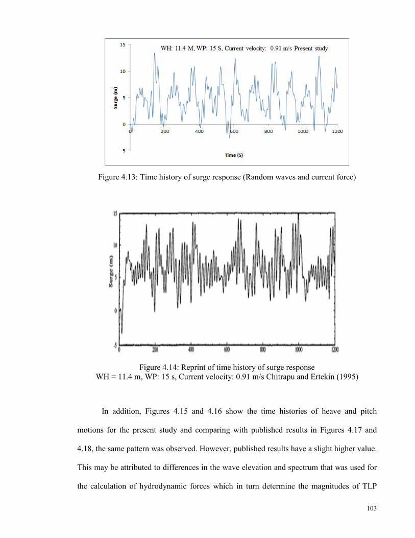
103
Figure 4.13: Time history of surge response (Random waves and current force)
Figure 4.14: Reprint of time history of surge response WH = 11.4 m, WP: 15 s, Current velocity: 0.91 m/s Chitrapu and Ertekin (1995)
In addition, Figures 4.15 and 4.16 show the time histories of heave and pitch
motions for the present study and comparing with published results in Figures 4.17 and
4.18, the same pattern was observed. However, published results have a slight higher value.
This may be attributed to differences in the wave elevation and spectrum that was used for
the calculation of hydrodynamic forces which in turn determine the magnitudes of TLP

104
degrees of freedom. As seen in Figures 4.19 and 4.20, there is a good similarity in trend
with a considerable difference in the value of tension variation for time histories of tendon
tension just as it was observed in regular wave simulation. Going by the power spectral
densities for surge, heave, pitch and tension variation in Figures 4.21, 4.22, 4.23 and 4.24
respectively, there are evidences to suggest that platform oscillation is governed
predominantly by surge natural frequency and wave forcing frequency. This fact was
established from the first prominent peak and cluster of peaks that coincides with the surge
and wave frequencies.
Figure 4.15: Time history of heave response (Random waves and Current force)

105
Figure 4.16: Time history of pitch response (Random waves and Current force)
Figure 4.17: Reprint of time history of heave response WH = 11.4 m, WP: 15 s, Current velocity: 0.91 m/s Chitrapu and Ertekin (1995)

106
Figure 4.18: Reprint of time history of pitch response WH = 11.4 m, WP: 15 s, Current velocity: 0.91 m/s Chitrapu and Ertekin (1995)
Figure 4.19: Time history of tension response

107
Figure 4.20: Reprint of time history of tension response WH = 11.4 m, WP: 15 s, Current velocity: 0.91 m/s Chitrapu and Ertekin (1995)
Figure 4.21: PSD of surge response (Present study)

108
Figure 4.22: PSD of heave response (Present study)
Figure 4.23: PSD of pitch response (Present study)
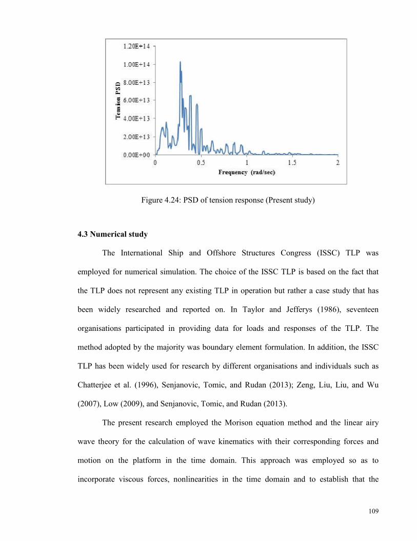
109
Figure 4.24: PSD of tension response (Present study)
4.3 Numerical study
The International Ship and Offshore Structures Congress (ISSC) TLP was
employed for numerical simulation. The choice of the ISSC TLP is based on the fact that
the TLP does not represent any existing TLP in operation but rather a case study that has
been widely researched and reported on. In Taylor and Jefferys (1986), seventeen
organisations participated in providing data for loads and responses of the TLP. The
method adopted by the majority was boundary element formulation. In addition, the ISSC
TLP has been widely used for research by different organisations and individuals such as
Chatterjee et al. (1996), Senjanovic, Tomic, and Rudan (2013); Zeng, Liu, Liu, and Wu
(2007), Low (2009), and Senjanovic, Tomic, and Rudan (2013).
The present research employed the Morison equation method and the linear airy
wave theory for the calculation of wave kinematics with their corresponding forces and
motion on the platform in the time domain. This approach was employed so as to
incorporate viscous forces, nonlinearities in the time domain and to establish that the

110
developed codes can be employed for the solution of hydrodynamic problems. The
platform principal parameters are summarized in Table 4.4 while hydrodynamic and
aerodynamic properties are also stated in Table 4.5
Table 4.4: Main particulars of ISSC TLP Senjanovic, Tomic, and Hadzic (2013) Parameters Value
Column spacing between centres 86.25 m Column diameter 16.88m
Pontoon width 7.50 m Pontoon height 10.50 m
Draft 35.00 m Displacement 5.346 x 10⁵ kN
Weight 3.973 x 10⁵ kN Total tether pretension 1.373 x 10⁵ kN
Longitudinal metacentric height 6.0 m Transverse metacentric height 6.0 m
Platform mass 40.5 x 10⁶ kg Roll mass moment of Inertia 82.37 x 10⁹ kg m2 Pitch mass moment of Inertia 82.37 x 10⁹ kg m2 Yaw mass moment of Inertia 98.07 x 10⁹ kg m2
Vertical position of COG above Keel 38.0 m Length of Mooring tethers, L 415.0 m
Vertical stiffness of combined tethers, EA/L 0.813 x 10⁶ kN/m Roll and Pitch effective stiffness, EIx/L, EIy/L 1.501 x 10⁹ kNm/rad
Table 4.5: Hydrodynamic and Aerodynamic Data Parameter Value
Sea Drag Coefficient, CD 1.0 Sea Inertia Coefficient, CM 2.0
Coefficient of Wind Drag, Ca 2.0 Surface current velocity (m/s) 1.05
Mean Wind Velocity (m/s) 50.10 Mass Density of Water 1025 kg/m3 Mass Density of Air, �a 1.25 kg/m3
Sea State parameters Hs = 12m, Tp = 14s
4.3.1 Comparison of natural periods of oscillation of the ISSC TLP
The first set of results aimed at ensuring that the motion response was as a result of
external forces and not from platform instability. This was achieved by summing vertical
forces in accordance with Equation 4.1 for static equilibrium at the undisturbed position.

111
The expected natural time period was reported in Gie and de Boom (1981) for the
uncoupled TLP and reproduced in Table 4.6 along with the analytical calculation for the
present study using Equation 4.2. From Table 4.6, we can see that results were in close
agreement with each other. This authenticate that the platform simulated is the same with
the one in the published result.
Table 4.6: Expected natural periods of motion Published Present Study Degree of Freedom Time (s) Frequency (rad/sec) Time (s) Frequency (rad/sec) Surge (Sway) 106.00 0.06 106.57 0.06 Heave 2.000 3.14 1.98 3.17 Roll (Pitch) 2.100 2.99 2.20 2.86 Yaw 86.00 0.07 85.50 0.07
4.3.2 Response of an uncoupled TLP in regular and random waves
The ISSC TLP was analysed for the Gulf of Mexico (GOM) sea conditions with
significant wave height of 12 m and spectral peak period of 14 s respectively. In order to
assess regular wave elevation, mathematical representation of regular wave in Section 3.3.1
was made use of. Random waves were characterized by summing individual regular wave
energy which resulted in what is known as wave spectrum. The random waves were
simulated based on the approach discussed in Section 3.3.2 of Chapter Three. Furthermore,
the spectrum used in long-crested sea failed to incorporate wave directionality, which
underestimate the true behaviour of the actual sea. The directional spectrum as calculated in
Section 3.3.2.1 was formulated from unidirectional spectrum with frequency independent
cosine power type energy spreading function. The simulation of wave profile was carried
out for a length of 5000 seconds with the time interval of 0.2 seconds. The results of the
wave profile shown in Figure 4.25 revealed regular wave idealisation have the same form
in time and space which is thought to be in contrast with the random wave characterization
which resembles what the ocean surface should look like because the shape, height and

112
length differ from wave to wave and practically impossible to distinguish each wave from
one another. Wave elevation profile for the directional random sea simulation comes with a
reduced magnitude. In addition, Figure 4.26 is the equivalent energy spectrum based on the
Pierson–Moskowitz model, (P.M) and the area under the curve gives the total energy for
the considered ocean environment.
Figure 4.25: Time history of wave surface profiles
Figure 4.26: Pierson–Moskowitz spectrum
-8
-6
-4
-2
0
2
4
6
8
4000 4050 4100 4150 4200 4250 4300
Wav
e p
rofi
le (
m)
Time (s)
WH 12 m, WP: 14 s
Regular wave Uniderctional random wave Directional random wave
0
10
20
30
0 0.5 1 1.5
Spe
ctra
l De
nsi
ty (
m2
rad
/se
c)
Frequency (rad/sec)
WH: 12 m, WP: 14 s
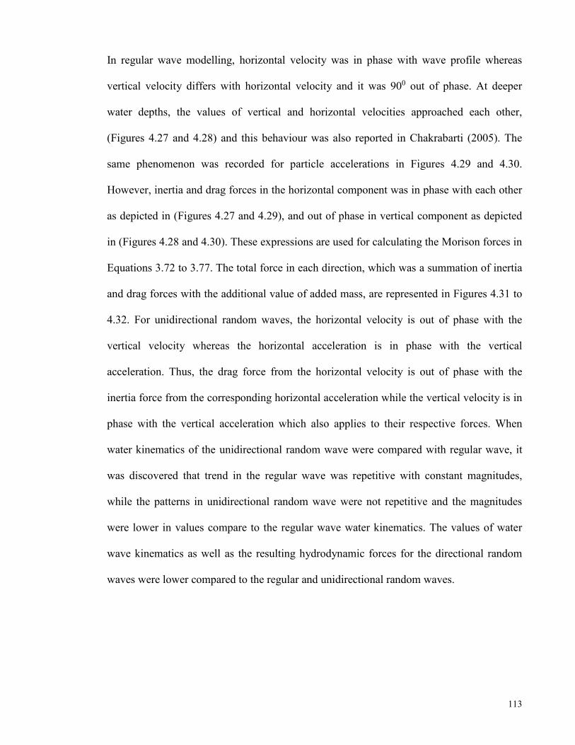
113
In regular wave modelling, horizontal velocity was in phase with wave profile whereas
vertical velocity differs with horizontal velocity and it was 900 out of phase. At deeper
water depths, the values of vertical and horizontal velocities approached each other,
(Figures 4.27 and 4.28) and this behaviour was also reported in Chakrabarti (2005). The
same phenomenon was recorded for particle accelerations in Figures 4.29 and 4.30.
However, inertia and drag forces in the horizontal component was in phase with each other
as depicted in (Figures 4.27 and 4.29), and out of phase in vertical component as depicted
in (Figures 4.28 and 4.30). These expressions are used for calculating the Morison forces in
Equations 3.72 to 3.77. The total force in each direction, which was a summation of inertia
and drag forces with the additional value of added mass, are represented in Figures 4.31 to
4.32. For unidirectional random waves, the horizontal velocity is out of phase with the
vertical velocity whereas the horizontal acceleration is in phase with the vertical
acceleration. Thus, the drag force from the horizontal velocity is out of phase with the
inertia force from the corresponding horizontal acceleration while the vertical velocity is in
phase with the vertical acceleration which also applies to their respective forces. When
water kinematics of the unidirectional random wave were compared with regular wave, it
was discovered that trend in the regular wave was repetitive with constant magnitudes,
while the patterns in unidirectional random wave were not repetitive and the magnitudes
were lower in values compare to the regular wave water kinematics. The values of water
wave kinematics as well as the resulting hydrodynamic forces for the directional random
waves were lower compared to the regular and unidirectional random waves.

114
Figure 4.27: Horizontal velocity on vertical column one
Figure 4.28: Vertical velocity on vertical column one
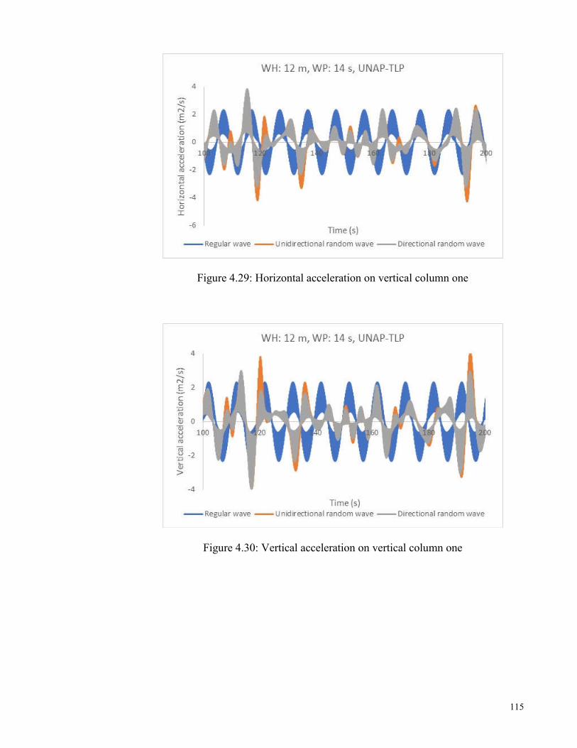
115
Figure 4.29: Horizontal acceleration on vertical column one
Figure 4.30: Vertical acceleration on vertical column one
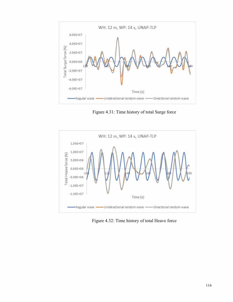
116
Figure 4.31: Time history of total Surge force
Figure 4.32: Time history of total Heave force

117
Figure 4.33: Time history of total Pitch force
The time history of the oscillation for the platform response in all degrees of freedom in
Figure 4.34 showed regular patterns for regular wave and stochastic for unidirectional and
directional random waves with platform being about the mean position and their values
were found to be small in relation to the wave elevation. One key difference is that the
surge magnitude in directional random wave is smaller compared to the outcome in
unidirectional random seas. The time histories of high frequency response of heave and
pitch motions are shown in Figures 4.35 and 4.36 with very high fluctuations. However,
their numerical values are very small compared to surge, due to the huge tension in the
tendons that restrain the vertical motions drastically. The time history of tendon tension
variation shown in Figure 4.37 come with a rapid fluctuation which was due to the high-
frequency motions and variable submergence associated with the vertical motions.
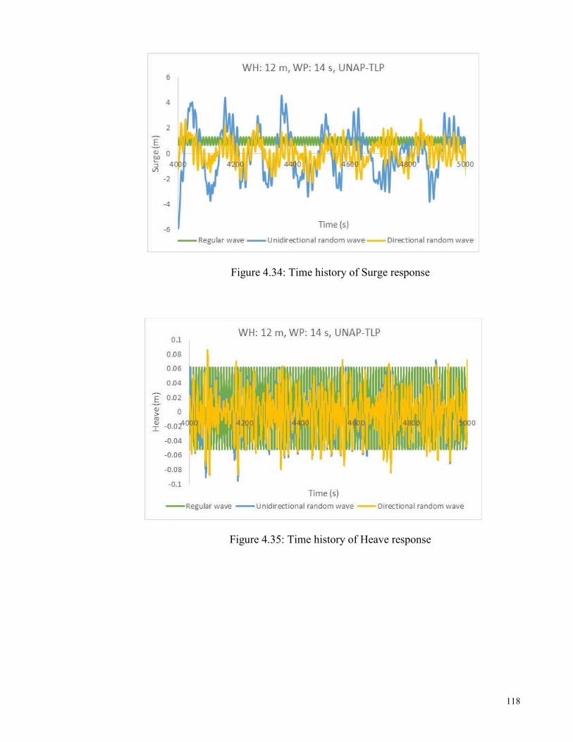
118
Figure 4.34: Time history of Surge response
Figure 4.35: Time history of Heave response

119
Figure 4.36: Time history of Pitch response
Figure 4.37: Time history of Tendon forces response
The only peak in the surge PSD for regular wave modelling in Figure 4.38 occurred at the
frequency of 0.64 rad/sec which is equivalent to time period of 9.76 secs. This time period
is the same with the zero up-crossing wave period for the wave frequency, and there is no
appearance of peak at surge natural time period as noticed in unidirectional and directional
random wave simulation. The heave PSD of the regular wave modelling in Figure 4.39

120
shows two peaks. The first peak which is the most prominent peak occurred at the
frequency of 0.64 rad/sec which happens to be the wave frequency while the second peak at
the frequency of 1.27 rad/sec did not fall at any natural period of oscillation of the TLP.
This can be regarded to have happened as a result of nonlinearity in the platform. The area
under the PSD curve is smaller compared to the surge PSD. For motion response in
unidirectional and directional random wave modelling, their first prominent peak was
around the surge natural frequency, which was absolutely absent in the case of regular
wave only and other cluster of peaks were noticed at the forcing frequency. The occurrence
of other peaks in Figure 4.40 apart from the peaks at surge and wave forcing frequencies
reveals the presence of nonlinearities and a very strong need for dynamic analysis.
In Figure 4.41, PSD of the tendon forces in regular wave modelling shows that the
first prominent peak is at wave frequency and the second peak is most likely due to the
nonlinearity. The PSD of the tendon tension variation of unidirectional and directional
random waves also revealed that surge natural frequency attracted much energy as this
affects other degrees of freedom as well as tendon tension. The lower peaks in the tendon
tension PSD confirm evidence of nonlinearities and tension variation in the tendons.
The implication of wave characterization is that vibration of the platform occurred
around the wave forcing frequency for regular wave and around surge natural frequency
and forcing frequency for random waves. The same trend of regular behaviour of the
platform in regular wave has been previously reported in Jameel, Oyejobi, Siddiqui, and
Ramli Sulong (2016) and Jain (1997). The time average and other statistical parameters for
each sea modelling were reported in Table 4.7. It is observed that the ratio of directional
RMS values of surge, heave, pitch and tension to unidirectional random seas values are
(1:2.08; 1:1.04; 1:1.12 and 1:1.03) which translate to 108%, 3.75%, 12.44% and 2.82%.
The unidirectional random sea produced higher motion responses to the tune of calculated

121
percentage due to the lack of wave directionality. Since the directional random waves
incorporated waves of different heights, frequencies, phase angle and directions, the wave
characterization and the platform response is recommended as an ideal result.
Figure 4.38: Power spectral density of Surge response
Figure 4.39: Power spectral density of Heave response
0
0.01
0.02
0.03
0.04
0.05
-0.1 0.1 0.3 0.5 0.7 0.9 1.1 1.3 1.5
He
ave
PSD
(m
2se
c/ra
d)
Frequency (rad/sec)
WH: 12 m, WP: 14 s, UNAP-TLP
Regular wave Unidirectional random wave Directional random wave

122
Figure 4.40: Power spectral density of Pitch response
Figure 4.41: Power spectral density of Tendon forces response
0
0.05
0.1
0.15
0.2
0.25
0 0.5 1 1.5 2
Pit
ch P
SD (
m2
sec/
rad
)
Frequency (rad/sec)
WH: 12 m, WP: 14 s, UNAP-TLP
Regular wave Unidirectional random wave Directional random wave
0.00E+00
5.00E+14
1.00E+15
1.50E+15
2.00E+15
0 0.5 1 1.5 2
Ten
sio
n f
orc
es
PSD
(m
2se
c/ra
d)
Frequency (rad/sec)
WH: 12 m, WP: 14 s, UNAP-TLP
Regular wave Unidirectional random wave Directional random wave
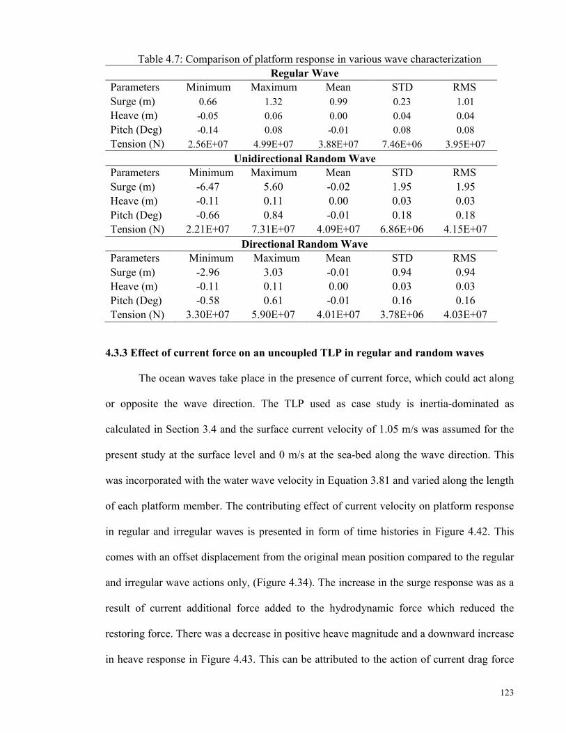
123
Table 4.7: Comparison of platform response in various wave characterization
Regular Wave Parameters Minimum Maximum Mean STD RMS
Surge (m) 0.66 1.32 0.99 0.23 1.01
Heave (m) -0.05 0.06 0.00 0.04 0.04
Pitch (Deg) -0.14 0.08 -0.01 0.08 0.08
Tension (N) 2.56E+07 4.99E+07 3.88E+07 7.46E+06 3.95E+07
Unidirectional Random Wave Parameters Minimum Maximum Mean STD RMS
Surge (m) -6.47 5.60 -0.02 1.95 1.95
Heave (m) -0.11 0.11 0.00 0.03 0.03
Pitch (Deg) -0.66 0.84 -0.01 0.18 0.18
Tension (N) 2.21E+07 7.31E+07 4.09E+07 6.86E+06 4.15E+07
Directional Random Wave Parameters Minimum Maximum Mean STD RMS
Surge (m) -2.96 3.03 -0.01 0.94 0.94
Heave (m) -0.11 0.11 0.00 0.03 0.03
Pitch (Deg) -0.58 0.61 -0.01 0.16 0.16
Tension (N) 3.30E+07 5.90E+07 4.01E+07 3.78E+06 4.03E+07
4.3.3 Effect of current force on an uncoupled TLP in regular and random waves
The ocean waves take place in the presence of current force, which could act along
or opposite the wave direction. The TLP used as case study is inertia-dominated as
calculated in Section 3.4 and the surface current velocity of 1.05 m/s was assumed for the
present study at the surface level and 0 m/s at the sea-bed along the wave direction. This
was incorporated with the water wave velocity in Equation 3.81 and varied along the length
of each platform member. The contributing effect of current velocity on platform response
in regular and irregular waves is presented in form of time histories in Figure 4.42. This
comes with an offset displacement from the original mean position compared to the regular
and irregular wave actions only, (Figure 4.34). The increase in the surge response was as a
result of current additional force added to the hydrodynamic force which reduced the
restoring force. There was a decrease in positive heave magnitude and a downward increase
in heave response in Figure 4.43. This can be attributed to the action of current drag force

124
that increased surge response in horizontal direction, increased buoyancy force and also
increased pretension force. The time history of pitch response in Figure 4.44 was not
adversely affected by the presence of current when compared with Figure 4.36 without
current force. Furthermore, the result of time history of variation of tension in the tendon is
represented in the Figure 4.45 with regular and stochastic pattern behaviours in the
oscillation for regular and irregular wave idealization. The current force caused a slight
reduction in the minimum tension and slight increase in the maximum value. However, the
mean and RMS values remained almost the same in both scenarios. This can be as a result
of counter-action between surge that increased surge motion and the negative increase in
heave motion.
Figure 4.42: Time history of Surge response (Wave and current forces)

125
Figure 4.43: Time history of Heave response (Wave and current forces)
Figure 4.44: Time history of Pitch response (Wave and current forces)
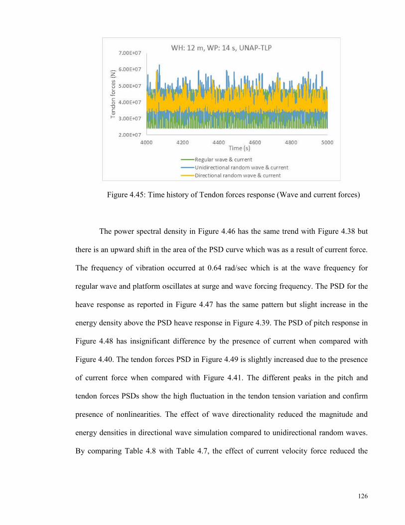
126
Figure 4.45: Time history of Tendon forces response (Wave and current forces)
The power spectral density in Figure 4.46 has the same trend with Figure 4.38 but
there is an upward shift in the area of the PSD curve which was as a result of current force.
The frequency of vibration occurred at 0.64 rad/sec which is at the wave frequency for
regular wave and platform oscillates at surge and wave forcing frequency. The PSD for the
heave response as reported in Figure 4.47 has the same pattern but slight increase in the
energy density above the PSD heave response in Figure 4.39. The PSD of pitch response in
Figure 4.48 has insignificant difference by the presence of current when compared with
Figure 4.40. The tendon forces PSD in Figure 4.49 is slightly increased due to the presence
of current force when compared with Figure 4.41. The different peaks in the pitch and
tendon forces PSDs show the high fluctuation in the tendon tension variation and confirm
presence of nonlinearities. The effect of wave directionality reduced the magnitude and
energy densities in directional wave simulation compared to unidirectional random waves.
By comparing Table 4.8 with Table 4.7, the effect of current velocity force reduced the

127
restoring force on the platform and this action increased the platform motion and causes
changes in the maximum and minimum tendon forces.
Figure 4.46: Power spectral density of Surge response (Wave and current forces)
Figure 4.47: Power spectral density of Heave response (Wave and current forces)

128
Figure 4.48: Power spectral density of Pitch response (Wave and current forces)
Figure 4.49: Power spectral density of Tendon response (Wave and current forces)

129
Table 4.8: Comparison of platform response in different wave and current forces
Regular Wave and Current force Parameters Minimum Maximum Mean STD RMS
Surge (m) 7.50 8.19 7.84 0.24 7.84
Heave (m) -0.14 0.00 -0.07 0.04 0.09
Pitch (Deg) -0.16 0.06 -0.04 0.08 0.09
Tension (N) 2.41E+07 4.77E+07 3.86E+07 7.91E+06 3.94E+07
Unidirectional random Wave and Current force Parameters Minimum Maximum Mean STD RMS
Surge (m) -7.15 14.06 4.22 3.38 5.40
Heave (m) -0.31 0.09 -0.04 0.05 0.06
Pitch (Deg) -0.71 0.76 -0.02 0.18 0.18
Tension (N) 1.99E+07 7.49E+07 4.07E+07 6.90E+06 4.13E+07
Directional random Wave and Current force Parameters Minimum Maximum Mean STD RMS
Surge (m) -4.34 11.67 4.40 2.64 5.13
Heave (m) -0.22 0.09 -0.03 0.04 0.05
Pitch (Deg) -0.58 0.50 -0.02 0.16 0.16
Tension (N) 3.28E+07 5.91E+07 4.01E+07 3.96E+06 4.03E+07
4.3.4 Effect of wind force on an uncoupled TLP in regular and random waves
The behaviour of TLP in wave - current - wind environment is discussed in this
section. The mean and fluctuating component winds have been detailed out in Section 3.4.4
and the results of their simulation are represented using time history, PSD and statistical
properties. With the magnitude of mean wind speed of 50.1 m/s for the GOM case study,
the platform was substantially influenced by this amount, resulting in a maximum departure
from the negative minimum surge value to the positive maximum value as shown for surge
time history. The behaviour of surge response in combined effect of regular wave, current
and wind force in Figure 4.50 is observed to be totally different from regular pattern as
witnessed for regular wave only, this can be accentuated to be the effect of fluctuating wind
component. The surge statistical values are all positive and stochastic in its behaviour for
unidirectional and directional waves. The positive response is as a result of drag forces
from current and wind forces.

130
The time history of the heave response is shown in Figure 4.51 with increase in negative
displacement direction due to the wind force. The higher increased values were as a result
of current and wind forces on the platform. In addition, the time history of pitch response in
regular and random waves along with current and wind forces is reported in Figure 4.52.
The pitch response did not significantly increase in value as much as surge and heave
responses increased. This suggests that undue discomfort due to rotational moment was not
envisaged on the platform. The time history of force variation in the tendon shown in
Figure 4.53 for the combined actions of regular wave, current and wind forces portrayed
regular shape but not completely sinusoidal in its form. It can be concluded that platform
under the influence of wave, current and wind forces experienced large excursion with an
increase in heave displacement but the variation of tension in the tendon is not as high as
the motion response.
Figure 4.50: Time history of Surge response (Wave, current and wind forces)
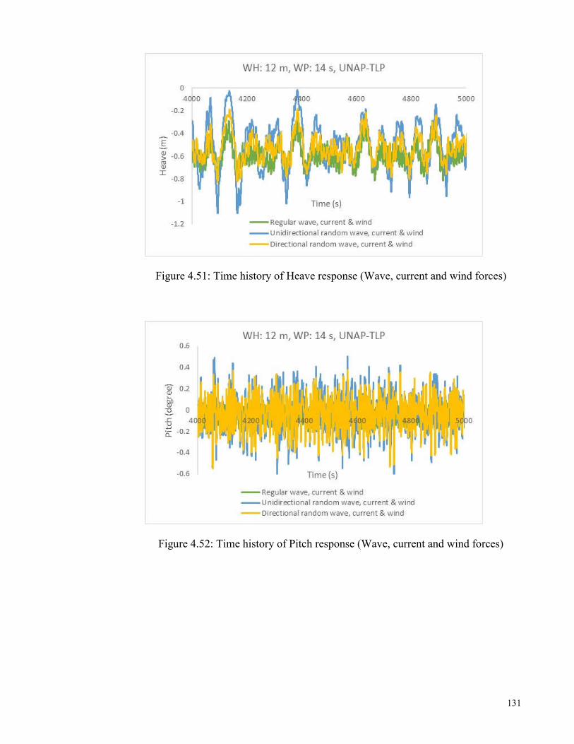
131
Figure 4.51: Time history of Heave response (Wave, current and wind forces)
Figure 4.52: Time history of Pitch response (Wave, current and wind forces)
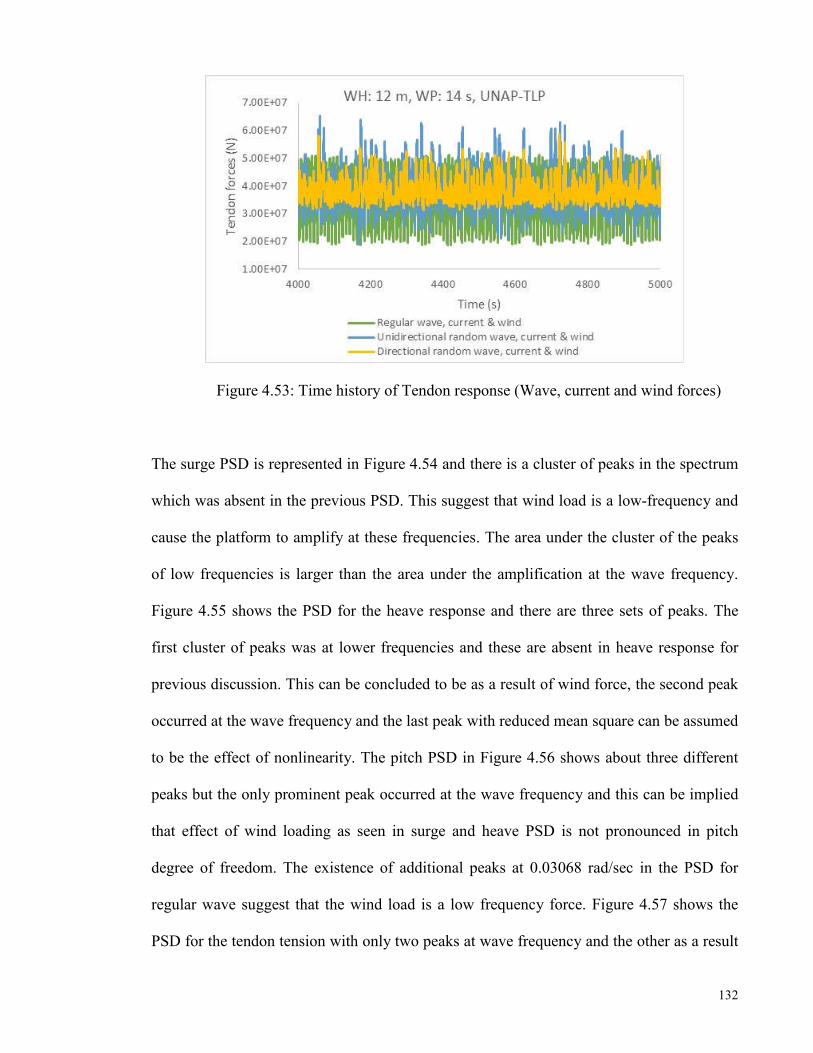
132
Figure 4.53: Time history of Tendon response (Wave, current and wind forces)
The surge PSD is represented in Figure 4.54 and there is a cluster of peaks in the spectrum
which was absent in the previous PSD. This suggest that wind load is a low-frequency and
cause the platform to amplify at these frequencies. The area under the cluster of the peaks
of low frequencies is larger than the area under the amplification at the wave frequency.
Figure 4.55 shows the PSD for the heave response and there are three sets of peaks. The
first cluster of peaks was at lower frequencies and these are absent in heave response for
previous discussion. This can be concluded to be as a result of wind force, the second peak
occurred at the wave frequency and the last peak with reduced mean square can be assumed
to be the effect of nonlinearity. The pitch PSD in Figure 4.56 shows about three different
peaks but the only prominent peak occurred at the wave frequency and this can be implied
that effect of wind loading as seen in surge and heave PSD is not pronounced in pitch
degree of freedom. The existence of additional peaks at 0.03068 rad/sec in the PSD for
regular wave suggest that the wind load is a low frequency force. Figure 4.57 shows the
PSD for the tendon tension with only two peaks at wave frequency and the other as a result

133
of variation in the tension for regular wave. The area under the PSD curve in this combined
loading is larger than the area under the PSD curve of regular wave and this indicates the
contribution of other forces. In unidirectional random wave, current and wind forces case,
the energy content in the surge PSD curve in Figure 4.54 had also increased when
compared with the surge PSD in Figures 4.38 and 4.46 for random wave only and random
wave and current force respectively. The PSD in Figures 4.54, 4.55, 4.56 and 4.57
respectively shows cluster of peaks at some very low frequencies of 0.02301, 0.03835,
0.05369 rad/sec, which is as a result of wind load with the first prominent peak at 0.08437
rad/sec. Subsequently, the platform is governed mainly at these frequencies which are
absent in the previous simulations. Thus, it is confirmed that TLP is sensitive to low-
frequency load. Furthermore, there were also prominent peaks in pitch and tendon tension
PSD, Figures 4.56 and 4.57 which can be attributed to outcomes of nonlinearities, variable
tendon tension and wind random load on the platform. While tension variation remains
almost unchanged, the motion responses behave differently in magnitude. It could be
concluded from Table 4.9 that maximum, minimum, mean and RMS motions greatly
increased when random wave, current and wind forces acted together except for tension
RMS variation that diminished due to what can be likened to countering effect between
surge and heave motion. Again, the wave directionality has reduced the energy content of
PSDs for surge, heave, pitch motions and tendon tension variation in Figures 4.54, 4.55,
4.56 and 4.57 when compared with their counterparts for unidirectional random wave in the
same Figures. The first set of the peaks in the PSDs of directional random waves are not
pronounced and their frequencies are very low which can be termed to be as a result of
wind forces on the platform. The first prominent peak and other cluster of peaks occurred at
the surge natural frequency and wave forcing frequencies respectively. Other peaks prove
the presence of nonlinearities and effect of tension variation in the tendons.

134
Low frequency structural response has been identified to be of great importance in the
dynamic behaviour of the TLP, Ahmad et al. (1997).
Figure 4.54: Power spectral density of Surge response (Wave, current and wind forces)
Figure 4.55: Power spectral density of Heave response (Wave, current and wind forces)
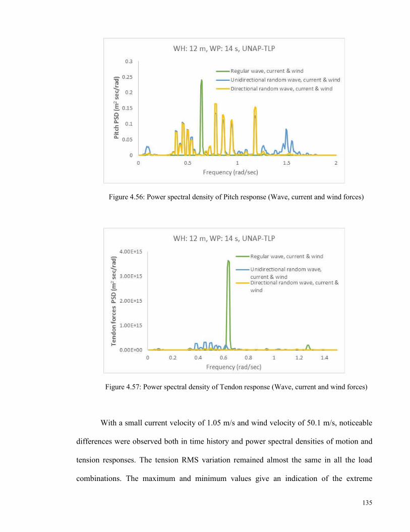
135
Figure 4.56: Power spectral density of Pitch response (Wave, current and wind forces)
Figure 4.57: Power spectral density of Tendon response (Wave, current and wind forces)
With a small current velocity of 1.05 m/s and wind velocity of 50.1 m/s, noticeable
differences were observed both in time history and power spectral densities of motion and
tension responses. The tension RMS variation remained almost the same in all the load
combinations. The maximum and minimum values give an indication of the extreme

136
response values for the platform while the Root Mean Square (RMS) is recommended for
the analysis of this type of problem since the simulation was carried out for a long period of
time and is of stochastic in nature. The principle of 68 - 95 - 99.7 rule in statistics field was
adopted to determine the percentage of values that lie around the mean value. Probability of
RMS values of the responses proved that 99.7 percent of the values were included and
these values are recommended for analysis purpose.
Table 4.9: Comparison of platform response in different wave, current and wind forces
Regular Wave, Current and Wind forces
Parameters Minimum Maximum Mean STD RMS
Surge (m) 16.96 24.73 21.70 1.65 21.76
Heave (m) -0.81 -0.29 -0.59 0.10 0.60
Pitch (Deg) -0.21 0.10 -0.04 0.08 0.09
Tension (N) 1.87E+07 5.15E+07 3.77E+07 9.78E+06 3.90E+07
Random Wave, Current and Wind forces
Parameters Minimum Maximum Mean STD RMS
Surge (m) 4.60 29.44 19.58 4.15 20.01
Heave (m) -1.12 0.02 -0.50 0.20 0.54
Pitch (Deg) -0.72 0.66 -0.03 0.18 0.18
Tension (N) 1.60E+07 7.25E+07 3.96E+07 7.51E+06 4.03E+07
Directional Wave, Current and Wind forces
Parameters Minimum Maximum Mean STD RMS
Surge (m) 11.07 26.11 20.40 2.44 20.55
Heave (m) -0.90 -0.14 -0.53 0.13 0.55
Pitch (Deg) -0.57 0.53 -0.03 0.16 0.16
Tension (N) 3.04E+07 5.99E+07 3.91E+07 4.37E+06 3.93E+07
4.4 Effect of the sea states on TLP motions
Table 4.10 shows eight different sea states from Siddiqui and Ahmad (2001) with
sea state parameters in descending order. Results of the effect of each state were simulated
with the Pierson-Moskowitz, (PM) spectrum. It was observed, as illustrated in Table 4.11,
that a decrease in each sea state (from severe to less severe sea state) leads to a decrease in
TLP motions. This trend is justified due to the fact that the PM spectrum is a function of
wave height and wave period. The difference between the RMS motion response in sea

137
state 1 and sea state 8 is quite large. Also, the higher sea state leads to increase in tension
value in the tendons as seen in Table 4.16. A comparison of RMS tendon tension between
sea state S1 and S8 showed that the difference in tendon tension for a least occurring sea
state and the most occurring sea state was small, about 13%. However, for the surge and
heave response, the differences are quite large, 296.98% and 257.14% respectively. This
can be interpreted that although surge and heave responses are the major cause of tension
variation in tendon, their combined influence over the tendon tension is considerably less.
The maximum and minimum tension values were determined from the combined
actions of initial pretension and environmental forces on the TLP. Very interestingly, the
maximum tension values largely determine the RMS tension values. Throughout the sea
states in Table 4.16, the higher the sea state parameters, the higher the maximum tension
value. Also, the lower the minimum tension value, the higher the RMS. The obtained
results are in order because the maximum tension is normally used to evaluate strength
criteria for tendons and their components while the minimum tendon tension in all the
tendons are expected to be positive and this was confirmed to be so.
Table 4.10: Simulated sea states (Siddiqui and Ahmad 2001) Sea State WH (m) WP (sec) Wind velocity (m/s) Probability of occurrence
S1 17.15 13.26 24.38 0.00000037 S2 15.65 12.66 23.29 0.00000238 S3 14.15 12.04 22.15 0.00001437 S4 12.65 11.39 20.94 0.00007980 S5 11.15 10.69 19.66 0.00040572 S6 9.65 9.94 18.29 0.00187129 S7 8.15 9.14 16.81 0.00773824 S8 6.65 8.26 15.18 0.02822122

138
Table 4.11: Effect of different wave heights and wave time periods on TLP motion
TLP Motions
Surge (m) Heave (m) Pitch (Deg)
Sea States Max Min STD RMS Max Min STD RMS Max Min STD RMS
S1 9.98 -7.20 2.98 3.02 0.13 -0.20 0.05 0.05 0.98 -0.69 0.21 0.21
S2 8.76 -6.70 2.63 2.66 0.12 -0.18 0.04 0.04 0.93 -0.65 0.20 0.20
S3 7.95 -6.31 2.29 2.30 0.12 -0.16 0.04 0.04 0.86 -0.60 0.18 0.18
S4 6.46 -5.77 1.95 1.96 0.12 -0.14 0.03 0.03 0.78 -0.54 0.17 0.17
S5 4.99 -5.04 1.64 1.65 0.10 -0.11 0.03 0.03 0.71 -0.51 0.15 0.15
S6 3.46 -4.12 1.34 1.34 0.09 -0.09 0.02 0.02 0.62 -0.47 0.14 0.14
S7 2.77 -3.17 1.04 1.04 0.07 -0.07 0.02 0.02 0.54 -0.44 0.12 0.12
S8 2.24 -2.26 0.76 0.76 0.05 -0.04 0.01 0.01 0.45 -0.40 0.11 0.11
4.4.1 Effect of current velocity on the sea states
A linearly varying current velocity of 1.05 m/s at the sea surface and 0 m/s at the
sea bed was assumed. With the same value of current velocity, as the sea state increased,
the surge RMS values also increased, as presented in Table 4.12. The current velocity in
conjunction with water particle along the same direction increased the drag force on the
platform. For sea states 1 and 2, the maximum heave values increased when wave and
current forces acted concurrently and started decreasing from sea state 3 to sea state 8.
Additionally, there was an increase in negative direction for the minimum heave motion.
The net RMS heave values were positive, increasing from the lowest sea state to the highest
sea state. The current force caused a decrease in maximum pitch rotational motion and an
increase in minimum pitch motion when compared with the action of random wave only.
However, there was a slight increase in pitch RMS values in lower sea states while higher
sea states decreased. This could be as a result of the decline in RMS tension values in
higher sea states and this correspondingly lead to increased RMS heave motion and
insignificant difference in pitch motion. Current force caused an increase in maximum
tension force values and a decrease in minimum tension force when it is compared with
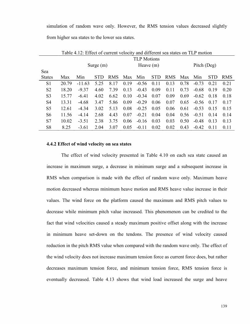
139
simulation of random wave only. However, the RMS tension values decreased slightly
from higher sea states to the lower sea states.
Table 4.12: Effect of current velocity and different sea states on TLP motion
TLP Motions
Surge (m) Heave (m) Pitch (Deg)
Sea States Max Min STD RMS Max Min STD RMS Max Min STD RMS
S1 20.79 -11.63 5.25 8.17 0.19 -0.56 0.11 0.13 0.78 -0.73 0.21 0.21
S2 18.20 -9.37 4.60 7.39 0.13 -0.43 0.09 0.11 0.73 -0.68 0.19 0.20
S3 15.77 -6.41 4.02 6.62 0.10 -0.34 0.07 0.09 0.69 -0.62 0.18 0.18
S4 13.31 -4.68 3.47 5.86 0.09 -0.29 0.06 0.07 0.65 -0.56 0.17 0.17
S5 12.61 -4.34 3.02 5.13 0.08 -0.25 0.05 0.06 0.61 -0.53 0.15 0.15
S6 11.56 -4.14 2.68 4.43 0.07 -0.21 0.04 0.04 0.56 -0.51 0.14 0.14
S7 10.02 -3.51 2.38 3.75 0.06 -0.16 0.03 0.03 0.50 -0.48 0.13 0.13
S8 8.25 -3.61 2.04 3.07 0.05 -0.11 0.02 0.02 0.43 -0.42 0.11 0.11
4.4.2 Effect of wind velocity on sea states
The effect of wind velocity presented in Table 4.10 on each sea state caused an
increase in maximum surge, a decrease in minimum surge and a subsequent increase in
RMS when comparison is made with the effect of random wave only. Maximum heave
motion decreased whereas minimum heave motion and RMS heave value increase in their
values. The wind force on the platform caused the maximum and RMS pitch values to
decrease while minimum pitch value increased. This phenomenon can be credited to the
fact that wind velocities caused a steady maximum positive offset along with the increase
in minimum heave set-down on the tendons. The presence of wind velocity caused
reduction in the pitch RMS value when compared with the random wave only. The effect of
the wind velocity does not increase maximum tension force as current force does, but rather
decreases maximum tension force, and minimum tension force, RMS tension force is
eventually decreased. Table 4.13 shows that wind load increased the surge and heave

140
responses substantially, but decreased the tendon tension slightly. Due to this counteracting
action, the net tendon tension has been decreased.
Table 4.13: Effect of wind velocity and different sea states TLP motion
TLP Motions
Surge (m) Heave (m) Pitch (Deg)
Sea States Max Min STD RMS Max Min STD RMS Max Min STD RMS
S1 17.78 -4.26 3.41 7.97 0.10 -0.49 0.08 0.12 0.80 -0.70 0.20 0.20
S2 15.92 -2.10 2.94 7.20 0.10 -0.40 0.07 0.10 0.76 -0.65 0.19 0.19
S3 14.37 -1.37 2.54 6.45 0.09 -0.33 0.06 0.08 0.73 -0.59 0.18 0.18
S4 12.43 -0.75 2.19 5.70 0.08 -0.25 0.05 0.06 0.69 -0.55 0.16 0.16
S5 10.50 -0.60 1.89 4.97 0.07 -0.19 0.04 0.05 0.64 -0.52 0.15 0.15
S6 8.61 -0.76 1.64 4.26 0.06 -0.14 0.03 0.04 0.59 -0.51 0.14 0.14
S7 7.30 -0.87 1.42 3.58 0.05 -0.10 0.02 0.03 0.53 -0.48 0.12 0.12
S8 6.13 -0.84 1.23 2.94 0.04 -0.07 0.02 0.02 0.45 -0.43 0.11 0.11
4.4.3 Effect of current and wind velocities on sea states
The effect of simultaneous action of current and wind velocities was studied next
and Table 4.14 shows there was an increase in the surge RMS value. This increase is
almost five times the response in random wave simulation only. In the same way, the effect
on the heave degree of freedom leads to a decrease in maximum heave motions, an increase
in minimum heave motions and a subsequent increase in heave RMS value. Also, there was
a decrease in maximum with an increase in minimum pitch values. These resulted into a
decrease in pitch RMS values in S1 – S5 and an increase in pitch RMS values for lower sea
states (S6 – S8). This trend is not out of order as current and wind forces cause steady
offsets and set-down. The pitch response, however, is not affected by these forces. The
values of maximum tension values in random wave, current and wind simulation depend on
each sea state while there was a decrease in minimum tension values across the sea states.
The steady forces reduced the RMS tension forces when compared with action of random

141
wave only, which is in line with simulation of random wave and current, and random wave
and wind forces respectively.
Table 4.14: Effect of current, wind velocities and different sea states on TLP motion
TLP Motions
Surge (m) Heave (m) Pitch (Deg)
Sea States Max Min STD RMS Max Min STD RMS Max Min STD RMS
S1 24.93 -7.97 5.21 12.25 0.12 -0.86 0.15 0.24 0.75 -0.72 0.20 0.21
S2 23.27 -6.51 4.67 11.37 0.10 -0.71 0.13 0.21 0.73 -0.67 0.19 0.19
S3 21.23 -4.18 4.08 10.45 0.10 -0.59 0.11 0.17 0.70 -0.61 0.18 0.18
S4 18.32 -2.91 3.51 9.48 0.08 -0.43 0.09 0.14 0.65 -0.55 0.17 0.17
S5 15.35 -1.50 2.97 8.45 0.07 -0.33 0.07 0.11 0.61 -0.53 0.15 0.15
S6 13.16 -0.56 2.53 7.39 0.05 -0.26 0.05 0.09 0.56 -0.52 0.14 0.14
S7 11.37 -0.61 2.19 6.31 0.04 -0.20 0.04 0.06 0.50 -0.48 0.12 0.13
S8 9.43 -1.18 1.96 5.21 0.03 -0.14 0.03 0.04 0.42 -0.44 0.11 0.11
4.4.4 Effect of one tendon missing in random waves and current forces
When one tendon was removed from a group of sixteen tendons at the corner one,
(Figure 4.85) due to its closeness to environmental and accidental loadings, there was an
increase of less than 1% in maximum and RMS surge values when compared with results
of intact TLP in Table 4.12. The values of heave RMS motion are believed to have reduced
as a result of the removal of one tendon to the values of 1.78 to 3.08% for sea state 1 to 5.
For lower sea states of 6 to 8, the RMS heave values remain unchanged. The removal of
one tendon in comparison to intact TLP in Table 4.12 caused an increase in maximum,
minimum and RMS pitch values with a percentage increase of RMS values between 8.13%
to 12.5% as presented in Table 4.15.
It can be said that the TLP becomes less stiff when a tendon was removed and this
lead to increase in maximum, minimum and RMS tension values between the values of 0.9
to 1.3%. The lower sea states suffered further increase in the tension value and this limits
the increase in motion response as shown in Table 4.16, compared to the higher sea states.
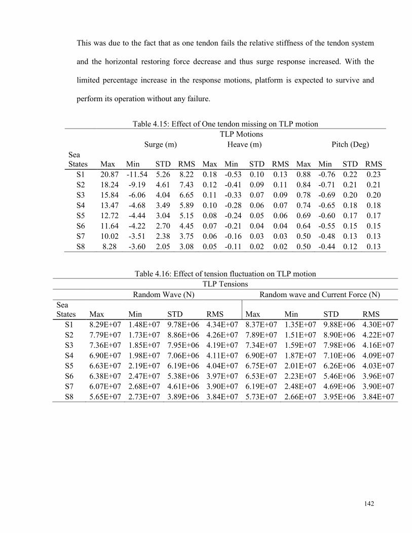
142
This was due to the fact that as one tendon fails the relative stiffness of the tendon system
and the horizontal restoring force decrease and thus surge response increased. With the
limited percentage increase in the response motions, platform is expected to survive and
perform its operation without any failure.
Table 4.15: Effect of One tendon missing on TLP motion
TLP Motions
Surge (m) Heave (m) Pitch (Deg)
Sea States Max Min STD RMS Max Min STD RMS Max Min STD RMS
S1 20.87 -11.54 5.26 8.22 0.18 -0.53 0.10 0.13 0.88 -0.76 0.22 0.23
S2 18.24 -9.19 4.61 7.43 0.12 -0.41 0.09 0.11 0.84 -0.71 0.21 0.21
S3 15.84 -6.06 4.04 6.65 0.11 -0.33 0.07 0.09 0.78 -0.69 0.20 0.20
S4 13.47 -4.68 3.49 5.89 0.10 -0.28 0.06 0.07 0.74 -0.65 0.18 0.18
S5 12.72 -4.44 3.04 5.15 0.08 -0.24 0.05 0.06 0.69 -0.60 0.17 0.17
S6 11.64 -4.22 2.70 4.45 0.07 -0.21 0.04 0.04 0.64 -0.55 0.15 0.15
S7 10.02 -3.51 2.38 3.75 0.06 -0.16 0.03 0.03 0.50 -0.48 0.13 0.13
S8 8.28 -3.60 2.05 3.08 0.05 -0.11 0.02 0.02 0.50 -0.44 0.12 0.13
Table 4.16: Effect of tension fluctuation on TLP motion
TLP Tensions
Random Wave (N) Random wave and Current Force (N)
Sea States Max Min STD RMS Max Min STD RMS
S1 8.29E+07 1.48E+07 9.78E+06 4.34E+07 8.37E+07 1.35E+07 9.88E+06 4.30E+07
S2 7.79E+07 1.73E+07 8.86E+06 4.26E+07 7.89E+07 1.51E+07 8.90E+06 4.22E+07
S3 7.36E+07 1.85E+07 7.95E+06 4.19E+07 7.34E+07 1.59E+07 7.98E+06 4.16E+07
S4 6.90E+07 1.98E+07 7.06E+06 4.11E+07 6.90E+07 1.87E+07 7.10E+06 4.09E+07
S5 6.63E+07 2.19E+07 6.19E+06 4.04E+07 6.75E+07 2.01E+07 6.26E+06 4.03E+07
S6 6.38E+07 2.47E+07 5.38E+06 3.97E+07 6.53E+07 2.23E+07 5.46E+06 3.96E+07
S7 6.07E+07 2.68E+07 4.61E+06 3.90E+07 6.19E+07 2.48E+07 4.69E+06 3.90E+07
S8 5.65E+07 2.73E+07 3.89E+06 3.84E+07 5.73E+07 2.66E+07 3.95E+06 3.84E+07

143
Table 4.16: Continued
TLP Tensions
Random wave and Wind Force (N) Random wave, current and Wind Forces (N)
Sea States Max Min STD RMS Max Min STD RMS
S1 8.22E+07 1.40E+07 9.61E+06 4.25E+07 8.44E+07 1.23E+07 1.00E+07 4.26E+07
S2 7.78E+07 1.44E+07 8.71E+06 4.19E+07 7.83E+07 1.48E+07 9.04E+06 4.19E+07
S3 7.26E+07 1.59E+07 7.83E+06 4.13E+07 7.24E+07 1.66E+07 8.09E+06 4.13E+07
S4 6.71E+07 1.85E+07 6.98E+06 4.07E+07 6.71E+07 1.78E+07 7.18E+06 4.07E+07
S5 6.55E+07 2.09E+07 6.16E+06 4.01E+07 6.57E+07 1.96E+07 6.31E+06 4.01E+07
S6 6.38E+07 2.30E+07 5.39E+06 3.95E+07 6.37E+07 2.18E+07 5.50E+06 3.95E+07
S7 6.10E+07 2.52E+07 4.64E+06 3.89E+07 6.09E+07 2.40E+07 4.72E+06 3.89E+07
S8 5.69E+07 2.71E+07 3.91E+06 3.84E+07 5.69E+07 2.53E+07 3.97E+06 3.84E+07
Table 4.16: Continued
One Tendon Missing
Random wave and Current Force (N) Sea States Max Min STD RMS
S1 8.40E+07 1.64E+07 9.93E+06 4.38E+07 S2 7.91E+07 1.61E+07 8.96E+06 4.30E+07 S3 7.38E+07 1.78E+07 8.05E+06 4.23E+07 S4 6.92E+07 1.94E+07 7.19E+06 4.16E+07 S5 6.76E+07 2.08E+07 6.38E+06 4.09E+07 S6 6.54E+07 2.28E+07 5.60E+06 4.02E+07 S7 6.19E+07 2.48E+07 4.69E+06 3.90E+07 S8 5.76E+07 2.63E+07 4.12E+06 3.89E+07
4.5 Verification of coupled TLP model
This section is concerned with the coupled model that has been simulated with the
same platform mass, water depth and the value of AE/L as reported for uncoupled TLP.
Based on past studies conducted by Taylor and Jefferys (1986), Chatterjee et al. (1996),
Senjanovic, Tomic, and Rudan (2013), very little was known about the tendon cross-
sectional area resulting in uncertainty regarding the cross-section type, (solid or hollow
cross-section). After several iterations, the simulation that gave close cross-section and
mass moment of inertia is the cross-sectional area of 0.4 metres square per corner and the
tendon diameter of 0.71 metres. This is similar to the tendon diameter used in MARLIN
and SNORRE A TLP respectively. The roll and pitch mass moment from the Abaqus finite
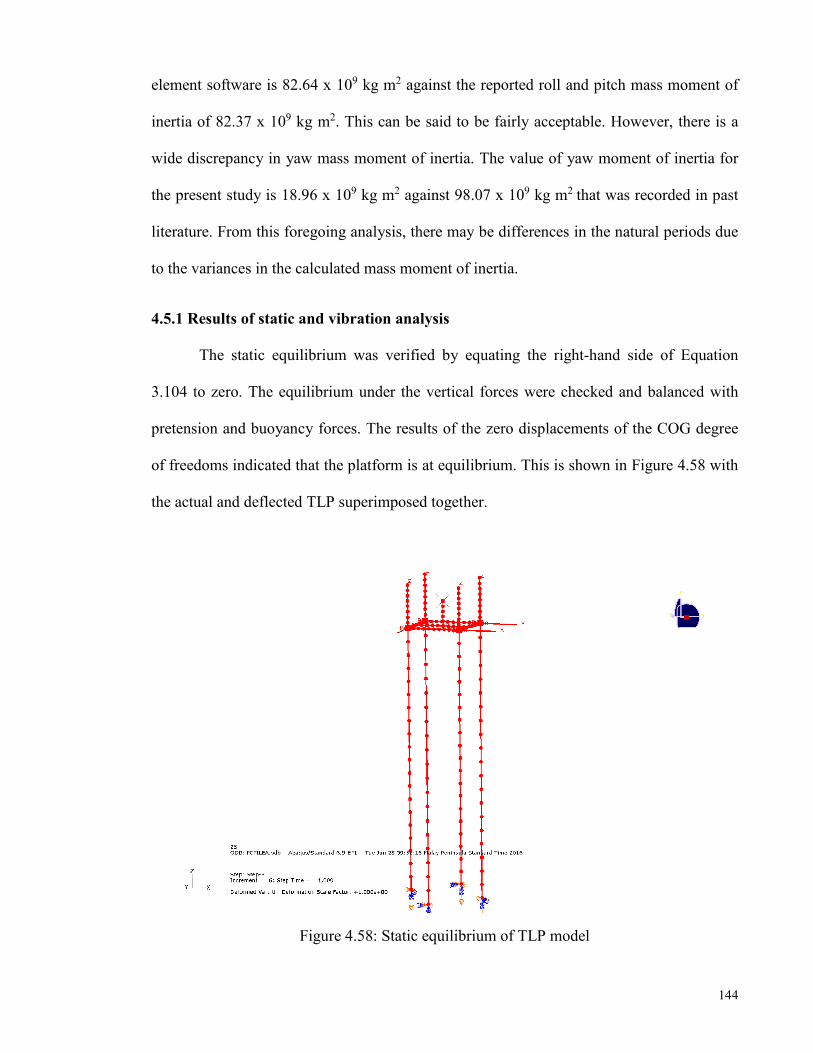
144
element software is 82.64 x 10⁹ kg m2 against the reported roll and pitch mass moment of
inertia of 82.37 x 10⁹ kg m2. This can be said to be fairly acceptable. However, there is a
wide discrepancy in yaw mass moment of inertia. The value of yaw moment of inertia for
the present study is 18.96 x 10⁹ kg m2 against 98.07 x 10⁹ kg m2 that was recorded in past
literature. From this foregoing analysis, there may be differences in the natural periods due
to the variances in the calculated mass moment of inertia.
4.5.1 Results of static and vibration analysis
The static equilibrium was verified by equating the right-hand side of Equation
3.104 to zero. The equilibrium under the vertical forces were checked and balanced with
pretension and buoyancy forces. The results of the zero displacements of the COG degree
of freedoms indicated that the platform is at equilibrium. This is shown in Figure 4.58 with
the actual and deflected TLP superimposed together.
Figure 4.58: Static equilibrium of TLP model

145
The undamped natural frequencies and mode shapes were calculated by the Lanczos
eigenvalues extraction method inside the Abaqus finite element software. The result of the
analytical calculation of the uncoupled natural period has been calculated and validated in
Section 4.3.1. Referring to Table 4.17, results of natural frequencies and periods for the
uncoupled TLP in the Abaqus software are stated. A comparison of Table 4.6 with Table
4.17 showed some level of agreement between the analytical and finite element method for
the calculation of natural frequencies.
Table 4.17: Uncoupled Eigenvalue output
Mode No Degree of Freedom Time (s) 1 Surge 112.04 2 Sway 112.04 3 Yaw 93.31
31 Roll 2.09 34 Pitch 2.08 38 Heave 2.03
The results of mode shapes 1, 2 and 3 that correspond to surge, sway and heave degrees of
freedom are presented in Figure 4.59 while Mode shapes 31, 34 and 38 correspond to roll,
pitch and heave degrees of freedom as shown in Figure 4.60. It was observed that the surge,
sway and yaw degrees of freedom are well above the dominant wave periods. Also, roll,
pitch and heave are below the prominent wave frequency because the important wave
natural periods have been identified to be between 3 to 25 seconds, Bhattacharyya et al.
(2003) and Taylor and Jefferys (1986).

146
Figure 4.59: Mode shapes of uncoupled TLP (Surge, Sway and Heave)
Figure 4.60: Mode shapes of uncoupled TLP (Roll, Pitch and Heave)
For the coupled TLP, the result of the eigenvalue output is presented in Table 4.18
with the omission of some mode numbers where it is believed that there is no strong
coupling between the TLP and the tendons. Mode shapes 1, 2 and 3 correspond to sway,
surge and yaw degrees of freedom and these are presented in Figure 4.61, while roll, pitch
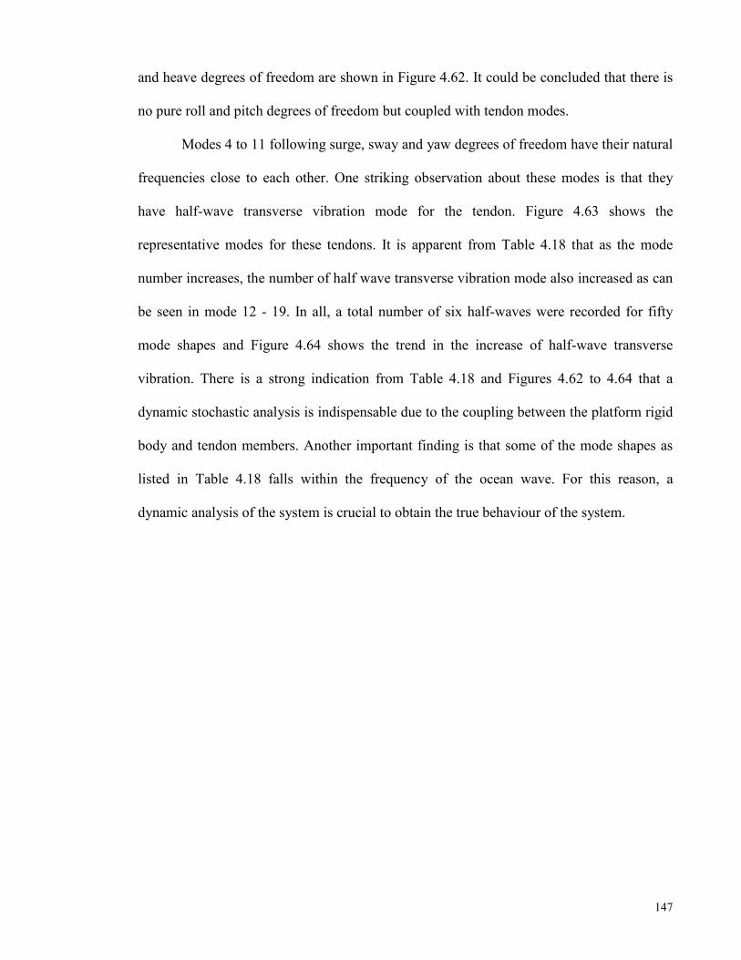
147
and heave degrees of freedom are shown in Figure 4.62. It could be concluded that there is
no pure roll and pitch degrees of freedom but coupled with tendon modes.
Modes 4 to 11 following surge, sway and yaw degrees of freedom have their natural
frequencies close to each other. One striking observation about these modes is that they
have half-wave transverse vibration mode for the tendon. Figure 4.63 shows the
representative modes for these tendons. It is apparent from Table 4.18 that as the mode
number increases, the number of half wave transverse vibration mode also increased as can
be seen in mode 12 - 19. In all, a total number of six half-waves were recorded for fifty
mode shapes and Figure 4.64 shows the trend in the increase of half-wave transverse
vibration. There is a strong indication from Table 4.18 and Figures 4.62 to 4.64 that a
dynamic stochastic analysis is indispensable due to the coupling between the platform rigid
body and tendon members. Another important finding is that some of the mode shapes as
listed in Table 4.18 falls within the frequency of the ocean wave. For this reason, a
dynamic analysis of the system is crucial to obtain the true behaviour of the system.

148
Table 4.18: Coupled eigenvalue output
Mode No Eigenvalue Frequency (rad/sec) Time (s) Remarks (Mode)
1 0.002 0.049 129.386 Sway
2 0.002 0.049 129.385 Surge
3 0.003 0.058 107.501 Yaw
4 0.405 0.636 9.877 Tendon
5 0.407 0.638 9.845 Tendon
6 0.407 0.638 9.843 Tendon
7 0.409 0.639 9.829 Tendon + Small Surge
8 0.443 0.666 9.439 Tendon
9 0.446 0.668 9.405 Tendon
10 0.446 0.668 9.404 Tendon
11 0.448 0.670 9.384 Tendon + Small Surge
12 1.661 1.289 4.875 Tendon
13 1.664 1.290 4.871 Tendon + Small Surge
23 3.872 1.968 3.193 Tendon
35 7.774 2.788 2.254 Tendon
36 8.723 2.954 2.127 Tendon + Roll
37 8.723 2.954 2.127 Tendon + Pitch
38 9.164 3.027 2.076 Heave
39 11.784 3.433 1.830 Tendon + small heave
40 11.788 3.433 1.830 Tendon
41 11.807 3.436 1.829 Tendon
42 11.808 3.436 1.829 Tendon
43 12.717 3.566 1.762 Tendon + small heave
50 17.995 4.242 1.481 Tendon
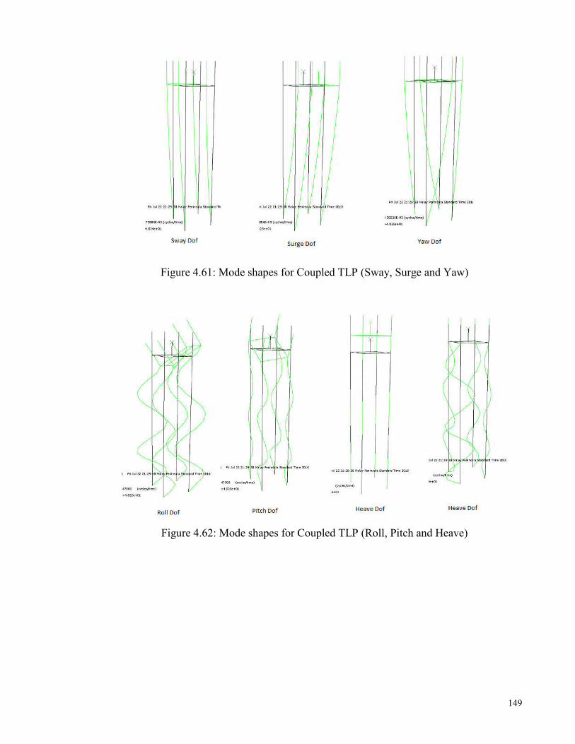
149
Figure 4.61: Mode shapes for Coupled TLP (Sway, Surge and Yaw)
Figure 4.62: Mode shapes for Coupled TLP (Roll, Pitch and Heave)
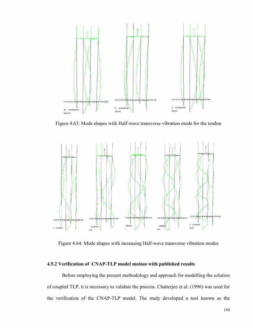
150
Figure 4.63: Mode shapes with Half-wave transverse vibration mode for the tendon
Figure 4.64: Mode shapes with increasing Half-wave transverse vibration modes
4.5.2 Verification of CNAP-TLP model motion with published results
Before employing the present methodology and approach for modelling the solution
of coupled TLP, it is necessary to validate the process. Chatterjee et al. (1996) was used for
the verification of the CNAP-TLP model. The study developed a tool known as the

151
DCATLP computational program that employed 3-dimensional finite beam elements and
these are programmed in the Sun FORTRAN software in their study. There may be slight
differences between the two models due to the manners TLP are modelled and noticeable
differences in the method of hydrodynamic force calculation.
Firstly, the platform hull and tendons are modelled as finite elements in the
DCATLP and not as a rigid body. Also, the DCATLP was developed to handle regular
waves and not random waves, so the validation will be for regular waves. Both models
employed the same integration method for the numerical analysis but there a was slight
difference in the force calculation. The ISSC TLP was used for the study comparison
although the tendon cross-section and diameter employed in the DCATLP are not explicit.
By comparing surge responses of the present study with Chatterjee et al. (1996) in
Figures 4.65, it was observed that the both magnitude and trend of the oscillation are the
same in the steady state in which the slight difference in the figures occurred in the
transient state. Figure 4.66 presents results of heave motion of the present study and
Chatterjee et al. (1996); the same trend and frequency of oscillation is observed in the two
figures. A likely explanation to the slight change in the magnitude can be attributed to
uncertainty in the tendon cross-section of the DCATLP model and different finite element
properties.
The results of pitch motion and tension variation in the tendons are not reported in
Chatterjee et al. (1996). However, the time histories of pitch and tension variation for the
present study are shown in Figures 4.67 and 4.68 respectively. Furthermore, the frequency
of platform vibration was not explicitly expressed in Chatterjee et al. (1996). However,
going by surge and heave time histories that were reported, one cycle of vibration is
completed in twenty seconds, which turns out to be a frequency value of 0.3142 rad/sec.

152
In the CNAP-TLP-2016 model, the frequency of platform vibration was calculated
by writing a Fast Fourier Transform program that converts the time histories to response
spectra as shown in Figures 4.69 and 4.70. Figures 4.69 and 4.70 show the peak frequency
of 0.3771 rad/sec which is approximately at the wave forcing frequency. This is in the
vicinity of visual calculation of frequency platform vibration for the DCATLP. It could be
said that wave forcing frequency governs the platform vibration.
Figure 4.65: Comparison of surge response: WH: 18 metres, WP: 17 secs, Current: 2 m/s, Wind: 30 m/s (Present study and Chatterjee et al. (1996))

153
Figure 4.66: Comparison of heave response: WH: 18 metres, WP: 17 secs, Current: 2 m/s, Wind: 30 m/s (Present study and Chatterjee et al. (1996))
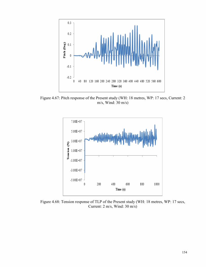
154
Figure 4.67: Pitch response of the Present study (WH: 18 metres, WP: 17 secs, Current: 2 m/s, Wind: 30 m/s)
Figure 4.68: Tension response of TLP of the Present study (WH: 18 metres, WP: 17 secs, Current: 2 m/s, Wind: 30 m/s)
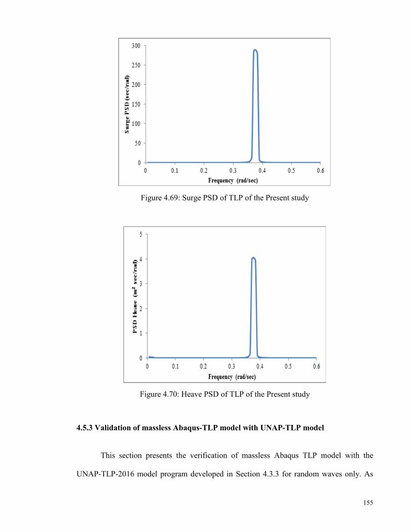
155
Figure 4.69: Surge PSD of TLP of the Present study
Figure 4.70: Heave PSD of TLP of the Present study
4.5.3 Validation of massless Abaqus-TLP model with UNAP-TLP model
This section presents the verification of massless Abaqus TLP model with the
UNAP-TLP-2016 model program developed in Section 4.3.3 for random waves only. As
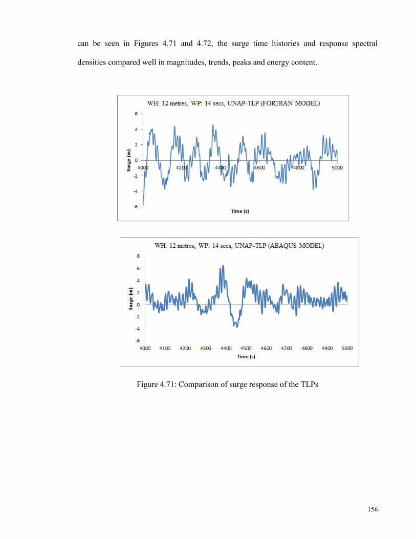
156
can be seen in Figures 4.71 and 4.72, the surge time histories and response spectral
densities compared well in magnitudes, trends, peaks and energy content.
Figure 4.71: Comparison of surge response of the TLPs
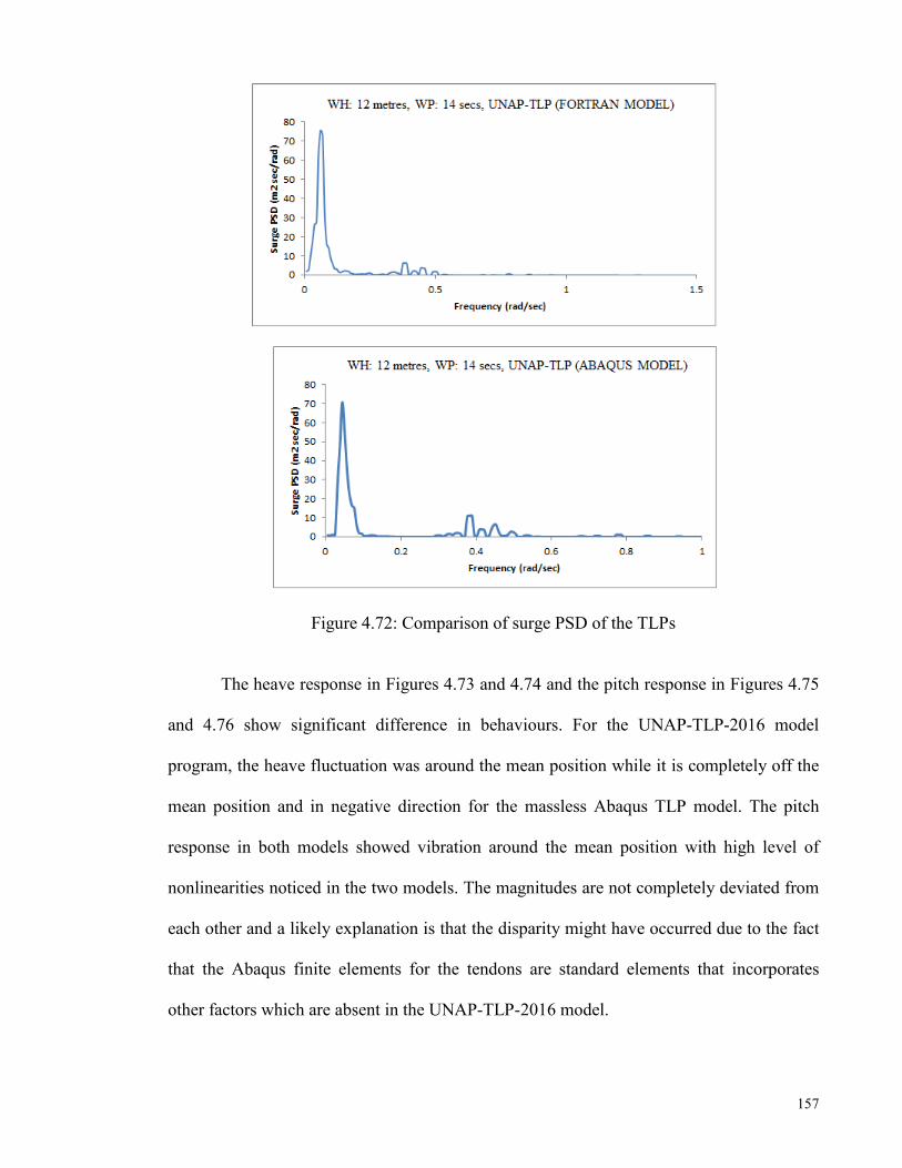
157
Figure 4.72: Comparison of surge PSD of the TLPs
The heave response in Figures 4.73 and 4.74 and the pitch response in Figures 4.75
and 4.76 show significant difference in behaviours. For the UNAP-TLP-2016 model
program, the heave fluctuation was around the mean position while it is completely off the
mean position and in negative direction for the massless Abaqus TLP model. The pitch
response in both models showed vibration around the mean position with high level of
nonlinearities noticed in the two models. The magnitudes are not completely deviated from
each other and a likely explanation is that the disparity might have occurred due to the fact
that the Abaqus finite elements for the tendons are standard elements that incorporates
other factors which are absent in the UNAP-TLP-2016 model.

158
Figure 4.73: Comparison of heave response of the TLPs
Figure 4.74: Comparison of heave PSD of the TLPs

159
Figure 4.75: Comparison of pitch response of the TLPs
Figure 4.76: Comparison of pitch PSD of the TLPs

160
The results of tendon tension response are shown in Figures 4.77 and 4.78. For the
cross-section of time histories and power spectral densities, their response shows some
degree of similarity in oscillation, magnitudes and in terms of peaks.
Figure 4.77: Comparison of tension response of the TLPs

161
Figure 4.78: Comparison of tension PSD of the TLPs
4.6 Effect of wave, current and wind loads on the response of CNAP-TLP model
The behaviour of the coupled TLP model was analysed for different load combinations
in 450 metres water depth. As a result of the zero-wave incident angle, the platform was
only activated in three degrees of freedom, which were surge, heave and pitch motions.
4.6.1 Surge time history
What is interesting in the modelling of TLP for random wave excitation only is that
the platform oscillates around the mean position. The random wave excitation simulated
from significant wave height of 12 m and peak time period of 14 s causes a maximum
displacement of 7.37 m and a minimum displacement of 3.84 m in the negative direction.
As seen in Figure 4.79, the oscillation is stochastic in nature, which follows the wave
elevation behaviour.
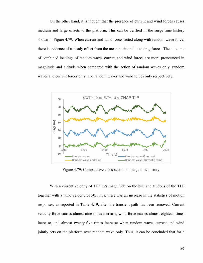
162
On the other hand, it is thought that the presence of current and wind forces causes
medium and large offsets to the platform. This can be verified in the surge time history
shown in Figure 4.79. When current and wind forces acted along with random wave force,
there is evidence of a steady offset from the mean position due to drag forces. The outcome
of combined loadings of random wave, current and wind forces are more pronounced in
magnitude and altitude when compared with the action of random waves only, random
waves and current forces only, and random waves and wind forces only respectively.
Figure 4.79: Comparative cross-section of surge time history
With a current velocity of 1.05 m/s magnitude on the hull and tendons of the TLP
together with a wind velocity of 50.1 m/s, there was an increase in the statistics of motion
responses, as reported in Table 4.19, after the transient path has been removed. Current
velocity force causes almost nine times increase, wind force causes almost eighteen times
increase, and almost twenty-five times increase when random wave, current and wind
jointly acts on the platform over random wave only. Thus, it can be concluded that for a
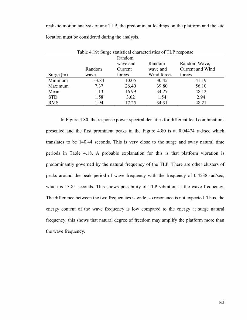
163
realistic motion analysis of any TLP, the predominant loadings on the platform and the site
location must be considered during the analysis.
Table 4.19: Surge statistical characteristics of TLP response
Surge (m) Random wave
Random wave and Current forces
Random wave and Wind forces
Random Wave, Current and Wind forces
Minimum -3.84 10.05 30.45 41.19 Maximum 7.37 26.40 39.80 56.10 Mean 1.13 16.99 34.27 48.12 STD 1.58 3.02 1.54 2.94 RMS 1.94 17.25 34.31 48.21
In Figure 4.80, the response power spectral densities for different load combinations
presented and the first prominent peaks in the Figure 4.80 is at 0.04474 rad/sec which
translates to be 140.44 seconds. This is very close to the surge and sway natural time
periods in Table 4.18. A probable explanation for this is that platform vibration is
predominantly governed by the natural frequency of the TLP. There are other clusters of
peaks around the peak period of wave frequency with the frequency of 0.4538 rad/sec,
which is 13.85 seconds. This shows possibility of TLP vibration at the wave frequency.
The difference between the two frequencies is wide, so resonance is not expected. Thus, the
energy content of the wave frequency is low compared to the energy at surge natural
frequency, this shows that natural degree of freedom may amplify the platform more than
the wave frequency.
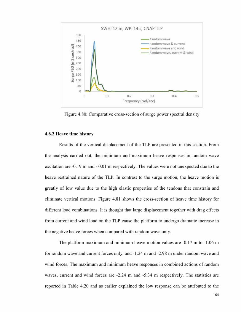
164
Figure 4.80: Comparative cross-section of surge power spectral density
4.6.2 Heave time history
Results of the vertical displacement of the TLP are presented in this section. From
the analysis carried out, the minimum and maximum heave responses in random wave
excitation are -0.19 m and - 0.01 m respectively. The values were not unexpected due to the
heave restrained nature of the TLP. In contrast to the surge motion, the heave motion is
greatly of low value due to the high elastic properties of the tendons that constrain and
eliminate vertical motions. Figure 4.81 shows the cross-section of heave time history for
different load combinations. It is thought that large displacement together with drag effects
from current and wind load on the TLP cause the platform to undergo dramatic increase in
the negative heave forces when compared with random wave only.
The platform maximum and minimum heave motion values are -0.17 m to -1.06 m
for random wave and current forces only, and -1.24 m and -2.98 m under random wave and
wind forces. The maximum and minimum heave responses in combined actions of random
waves, current and wind forces are -2.24 m and -5.34 m respectively. The statistics are
reported in Table 4.20 and as earlier explained the low response can be attributed to the

165
high stiffness of the tendon together with the tendon damping that restrains the motion in
vertical mode.
Figure 4.81: Comparative cross-section of heave time history
Table 4.20: Heave statistical characteristics of TLP Response
Heave (m) Random wave
Random wave and Current forces
Random wave and Wind forces
Random Wave, Current and Wind forces
Minimum -0.19 -1.06 -2.98 -5.34 Maximum -0.01 -0.17 -1.24 -2.24 Mean -0.04 -0.45 -1.71 -3.34 STD 0.02 0.16 0.27 0.54 RMS 0.05 0.48 1.73 3.38
From Figure 4.82, it is clear that there is a strong coupling between surge and heave
degrees of freedom. This is because the first dominant peaks in all load combinations
occurs at surge natural time period and other noticeable cluster of peaks occur around wave
frequency. The strong coupling is due to the fact that wave direction is along the surge
direction and also the surge offset causes set down along the heave direction.
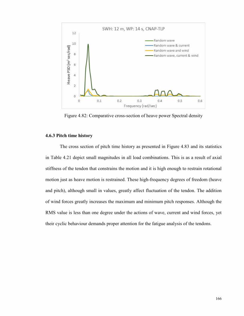
166
Figure 4.82: Comparative cross-section of heave power Spectral density
4.6.3 Pitch time history
The cross section of pitch time history as presented in Figure 4.83 and its statistics
in Table 4.21 depict small magnitudes in all load combinations. This is as a result of axial
stiffness of the tendon that constrains the motion and it is high enough to restrain rotational
motion just as heave motion is restrained. These high-frequency degrees of freedom (heave
and pitch), although small in values, greatly affect fluctuation of the tendon. The addition
of wind forces greatly increases the maximum and minimum pitch responses. Although the
RMS value is less than one degree under the actions of wave, current and wind forces, yet
their cyclic behaviour demands proper attention for the fatigue analysis of the tendons.

167
Figure 4.83: Comparative cross-section of pitch time history
Table 4.21: Pitch statistical characteristics of TLP response
Pitch (Deg) Random wave
Random wave and Current forces
Random wave and Wind forces
Random Wave, Current and Wind forces
Minimum -0.06 -0.12 -0.21 -0.39 Maximum 0.10 0.38 1.67 2.58 Mean 0.00 0.02 0.18 0.33 STD 0.02 0.07 0.29 0.50 RMS 0.02 0.07 0.34 0.60
The pitch power spectra shown in Figure 4.84 follow the same trend of noticeable peaks at
surge natural frequency and at wave forcing frequency. This further strengthened the
evidence for coupling and nonlinearities embedded in the TLP system.

168
Figure 4.84: Comparative cross-section of pitch power spectral density
4.6.4 Tendon tension time history
Having discussed the TLP motion, the high-frequency tension fluctuation in the
tendon is discussed next. This occurred due to variable submergence, large offset from
environmental forces that changed the tension at every time instant in the tendon. Besides
this, time varying forces in the tendon and unequal set-down that accompany the offset
caused the tension to vary from tendon to tendon.
In this study, equivalent tendon representation was used and the top tension in the
corner, C1 (Figure 4.85) in the random wave, random wave and current, random wave,
current and wind forces simulation is recorded in Table 4.22.

169
Figure 4.85: Arrangement of TLP tendon
Table 4.22: Tension statistical characteristics of TLP response
Tension (N) Random wave
Random wave and Current forces
Random wave and Wind forces
Random Wave, Current and Wind forces
Minimum 2.37E+07 2.49E+07 1.99E+07 2.41E+07 Maximum 4.38E+07 4.58E+07 6.74E+07 6.32E+07 Mean 3.38E+07 3.47E+07 3.83E+07 3.85E+07 STD 3.19E+06 3.16E+06 6.17E+06 5.84E+06 RMS 3.40E+07 3.48E+07 3.88E+07 3.89E+07
The current drag force increases both minimum and maximum tension in the tendon
while the wind drag force increased the maximum tension and decreased the minimum
tension. The effects of load combination on the response of tendon are represented in time
history (Figure 4.86). In all, the nonlinearity in the TLP was confirmed by the presence of
fluctuation in the time history of tendon tension. Although, the motion behaviour greatly
increased when current and wind forces were added to wave force as previously discussed,
the difference in tension RMS was not so much as there is only 2.4%, 14.12%, and 14.41%
increase in tension when random wave and current forces, random wave and wind forces,
and joint occurrence of random wave, current and wind forces act together over random
wave simulation only. it can be said that the initial tendon pretension and buoyancy forces

170
were sufficient in carrying the imposed structural load and resisting the environmental
forces on the TLP structure.
Figure 4.86: Comparative cross-section of tension time history
Apart from peaks at surge and wave frequencies, there were other peaks in the
tendon power spectra model as depicted in Figure 4.87. These were the result of
nonlinearities in the platform. The tension fluctuation in the tendon is directly influenced
by the heaving on the platform. It can be seen in Figure 4.87 that the energy content under
the actions of random wave, current and wind forces were considerably larger than the
random wave simulation only due to the drag load effects and the rapid fluctuations caused
by variable submergence and tension fluctuation.
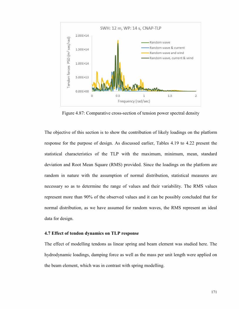
171
Figure 4.87: Comparative cross-section of tension power spectral density
The objective of this section is to show the contribution of likely loadings on the platform
response for the purpose of design. As discussed earlier, Tables 4.19 to 4.22 present the
statistical characteristics of the TLP with the maximum, minimum, mean, standard
deviation and Root Mean Square (RMS) provided. Since the loadings on the platform are
random in nature with the assumption of normal distribution, statistical measures are
necessary so as to determine the range of values and their variability. The RMS values
represent more than 90% of the observed values and it can be possibly concluded that for
normal distribution, as we have assumed for random waves, the RMS represent an ideal
data for design.
4.7 Effect of tendon dynamics on TLP response
The effect of modelling tendons as linear spring and beam element was studied here. The
hydrodynamic loadings, damping force as well as the mass per unit length were applied on
the beam element, which was in contrast with spring modelling.

172
For the surge response, the values were in close range for both coupled and uncoupled
models as reported in Table 4.23. The percentage difference in maximum, minimum and
RMS absolute values between the coupled and uncoupled analysis of TLP was found to be
14.01%, 3.47% and 26.55%. Coupled TLP had additional loadings incorporated into the
equation of motion and this made the surge motion to be higher compared to result of surge
from uncoupled TLP. The response was also properly damped as a result of hydrodynamic
damping forces from the tendons. The heave response is a high frequency response and due
to the high axial stiffness of the tendon that restrains the vertical motion, the heave
response is low when compared to the surge motion. The highest response values were
recorded when the tendon was modelled as linear spring with stiffness only against the non-
linear beam element that incorporate tendon dynamics. The percentage difference in the
absolute maximum, minimum and RMS heave values are 200%, 100% and 256.52%
respectively. A possible reason for the higher response in linear spring tendon might be due
to the fact that hydrodynamic damping from the tendon is absent. In addition, the negative
heave value was also due to the induced set-down from large offset of the platform.
The magnitudes of the statistical pitch response are low and the highest RMS value was
also observed when tendons were modelled as linear spring against non-linear beam
element. This is high-frequency response that influenced the maximum and minimum
tensions in the tendon although, discomfort was not envisaged on the platform deck since
pitch values were small. The percentage difference in the absolute maximum, minimum
and RMS pitch values are 173%, 400% and 331.82% respectively. The results in this
section indicated that the uncoupled model without tendon dynamics predicted surge
response fairly but heave and pitch responses had huge discrepancies. This can be assumed
to be a result of the linear spring modelling adopted for the tendon.

173
Table 4.23: Comparison of statistical motion characteristics of TLP response TLP Model Uncoupled Coupled Uncoupled Coupled Uncoupled Coupled Parameters Surge (m) Heave (m) Pitch (Degree) Minimum -3.71 -3.84 -0.38 -0.19 -0.30 -0.06 Maximum 6.47 7.37 0.05 -0.01 0.26 0.10
Mean 0.70 1.13 -0.15 -0.04 -0.02 0.02 STD 1.36 1.58 0.06 0.02 0.09 0.02 RMS 1.53 1.94 0.16 0.05 0.10 0.02
Table 4.24: Comparison of statistical tension characteristics of TLP response TLP Model Uncoupled Coupled Uncoupled Coupled Uncoupled Coupled Uncoupled Coupled Parameters Tendon 1 Tendon 2 Tendon 3 Tendon 4 Minimum -3.94E+06 2.37E+07 3.73E+06 2.06E+07 -1.00E+07 2.19E+07 -2.13E+06 2.39E+07 Maximum 7.22E+07 4.38E+07 7.13E+07 4.31E+07 7.29E+07 4.48E+07 7.01E+07 4.43E+07 Mean 3.30E+07 3.38E+07 3.51E+07 3.33E+07 3.30E+07 3.38E+07 3.51E+07 3.34E+07 STD 1.17E+07 3.19E+06 1.16E+07 3.80E+06 1.16E+07 3.79E+06 1.12E+07 3.24E+06 RMS 3.50E+07 3.40E+07 3.70E+07 3.35E+07 3.49E+07 3.40E+07 3.68E+07 3.35E+07
There was an unequal tension distribution in the tendons as presented in Table 4.24.
This was said earlier to be as a result of unequal set-down. The maximum tension variation
in the linear spring models without tendon dynamics were higher and the minimum tension
variation was lower compared to the beam elements with tendon dynamics. The RMS
tension values were approximately in the same the range as the initial tension values. The
minimum and maximum tension values are important because they determine what the
strength of the tendon materials should be. The linear spring model produced the highest
maximum tension and negative minimum tension in some of the tendons. In the beam
elements of tendon modelling, the maximum and minimum tension values are positive and
of smaller magnitude when compared with linear spring elements.
4.8 TLP response in constant wave height and varying wave period
The parametric study on coupled ISSC TLP was carried out for random wave and
current forces simulation. The geometric data is the same with Table 4.5 for constant wave
height of 12 metres. The wave periods of 10, 12, 14 and 16 seconds that fall within the
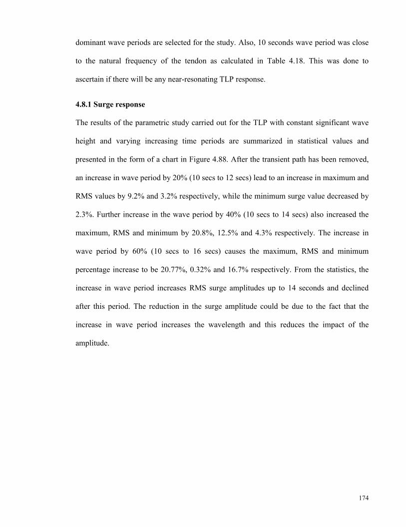
174
dominant wave periods are selected for the study. Also, 10 seconds wave period was close
to the natural frequency of the tendon as calculated in Table 4.18. This was done to
ascertain if there will be any near-resonating TLP response.
4.8.1 Surge response
The results of the parametric study carried out for the TLP with constant significant wave
height and varying increasing time periods are summarized in statistical values and
presented in the form of a chart in Figure 4.88. After the transient path has been removed,
an increase in wave period by 20% (10 secs to 12 secs) lead to an increase in maximum and
RMS values by 9.2% and 3.2% respectively, while the minimum surge value decreased by
2.3%. Further increase in the wave period by 40% (10 secs to 14 secs) also increased the
maximum, RMS and minimum by 20.8%, 12.5% and 4.3% respectively. The increase in
wave period by 60% (10 secs to 16 secs) causes the maximum, RMS and minimum
percentage increase to be 20.77%, 0.32% and 16.7% respectively. From the statistics, the
increase in wave period increases RMS surge amplitudes up to 14 seconds and declined
after this period. The reduction in the surge amplitude could be due to the fact that the
increase in wave period increases the wavelength and this reduces the impact of the
amplitude.
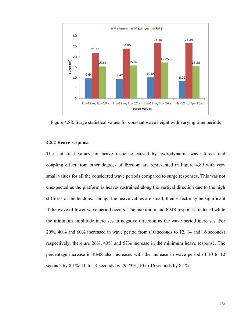
175
Figure 4.88: Surge statistical values for constant wave height with varying time periods
4.8.2 Heave response
The statistical values for heave response caused by hydrodynamic wave forces and
coupling effect from other degrees of freedom are represented in Figure 4.89 with very
small values for all the considered wave periods compared to surge responses. This was not
unexpected as the platform is heave- restrained along the vertical direction due to the high
stiffness of the tendons. Though the heave values are small, their effect may be significant
if the wave of lower wave period occurs. The maximum and RMS responses reduced while
the minimum amplitude increases in negative direction as the wave period increases. For
20%, 40% and 60% increased in wave period from (10 seconds to 12, 14 and 16 seconds)
respectively, there are 26%, 43% and 57% increase in the minimum heave response. The
percentage increase in RMS also increases with the increase in wave period of 10 to 12
seconds by 8.1%; 10 to 14 seconds by 29.73%; 10 to 16 seconds by 8.1%.
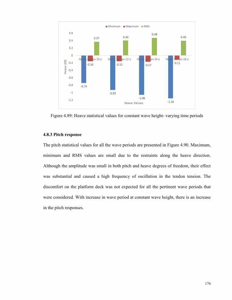
176
Figure 4.89: Heave statistical values for constant wave height- varying time periods
4.8.3 Pitch response
The pitch statistical values for all the wave periods are presented in Figure 4.90. Maximum,
minimum and RMS values are small due to the restraints along the heave direction.
Although the amplitude was small in both pitch and heave degrees of freedom, their effect
was substantial and caused a high frequency of oscillation in the tendon tension. The
discomfort on the platform deck was not expected for all the pertinent wave periods that
were considered. With increase in wave period at constant wave height, there is an increase
in the pitch responses.

177
Figure 4.90: Pitch statistical values for constant wave height- varying time periods
4.8.4 Tendon tension response
This section studied the variation in tendon tension due to the combined effects of
pretension, wave and current forces. The magnitude of the high frequency (Heave and
Pitch) motions was small but their contribution was a key factor towards the high tension
fluctuation. It was noticed that there was an unequal tension distribution in each tendon leg
as represented by corner 1, 2, 3 and 4 (Figure 4.85) and this might have occurred due to the
unequal set-down. The statistical tension parameter in corner, C1 is represented in Figure
4.91 for the parametric study. At constant wave height with increasing wave period, the
minimum tension decreased, maximum tension values increased slightly and RMS
remained almost unchanged for all the wave period increment. The variation within the
tendon tension was within the limits and not susceptible to any unrealistic behaviours.
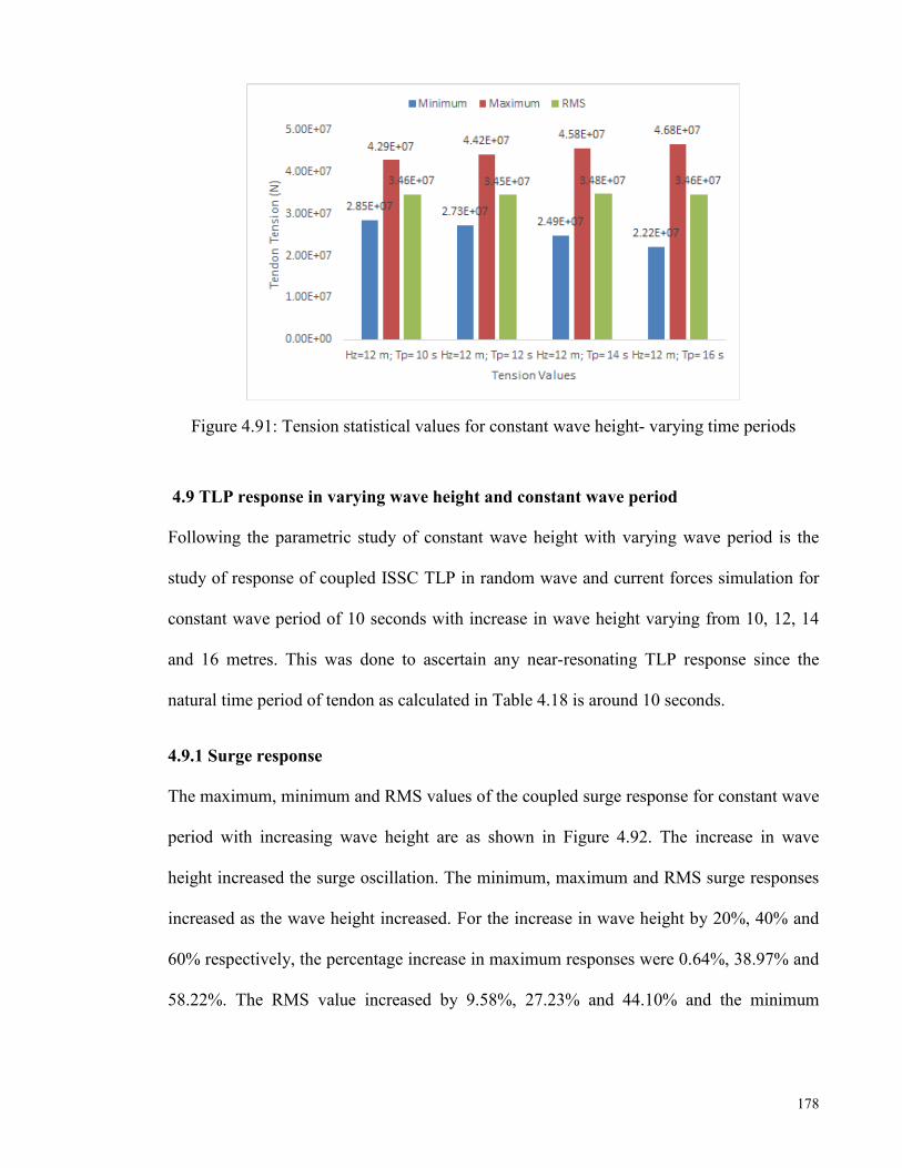
178
Figure 4.91: Tension statistical values for constant wave height- varying time periods
4.9 TLP response in varying wave height and constant wave period
Following the parametric study of constant wave height with varying wave period is the
study of response of coupled ISSC TLP in random wave and current forces simulation for
constant wave period of 10 seconds with increase in wave height varying from 10, 12, 14
and 16 metres. This was done to ascertain any near-resonating TLP response since the
natural time period of tendon as calculated in Table 4.18 is around 10 seconds.
4.9.1 Surge response
The maximum, minimum and RMS values of the coupled surge response for constant wave
period with increasing wave height are as shown in Figure 4.92. The increase in wave
height increased the surge oscillation. The minimum, maximum and RMS surge responses
increased as the wave height increased. For the increase in wave height by 20%, 40% and
60% respectively, the percentage increase in maximum responses were 0.64%, 38.97% and
58.22%. The RMS value increased by 9.58%, 27.23% and 44.10% and the minimum
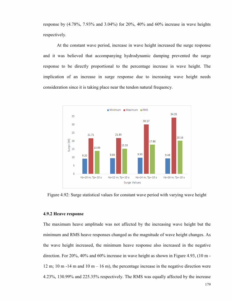
179
response by (4.78%, 7.93% and 3.04%) for 20%, 40% and 60% increase in wave heights
respectively.
At the constant wave period, increase in wave height increased the surge response
and it was believed that accompanying hydrodynamic damping prevented the surge
response to be directly proportional to the percentage increase in wave height. The
implication of an increase in surge response due to increasing wave height needs
consideration since it is taking place near the tendon natural frequency.
Figure 4.92: Surge statistical values for constant wave period with varying wave height
4.9.2 Heave response
The maximum heave amplitude was not affected by the increasing wave height but the
minimum and RMS heave responses changed as the magnitude of wave height changes. As
the wave height increased, the minimum heave response also increased in the negative
direction. For 20%, 40% and 60% increase in wave height as shown in Figure 4.93, (10 m -
12 m; 10 m -14 m and 10 m – 16 m), the percentage increase in the negative direction were
4.23%, 130.99% and 225.35% respectively. The RMS was equally affected by the increase
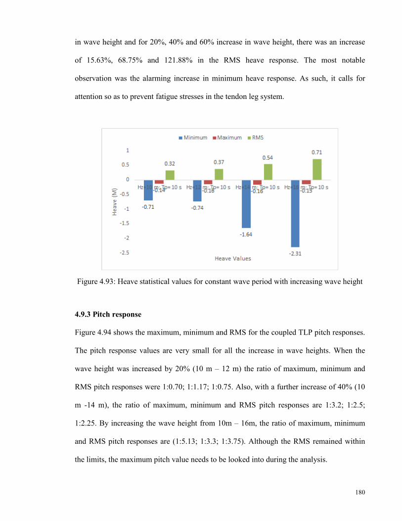
180
in wave height and for 20%, 40% and 60% increase in wave height, there was an increase
of 15.63%, 68.75% and 121.88% in the RMS heave response. The most notable
observation was the alarming increase in minimum heave response. As such, it calls for
attention so as to prevent fatigue stresses in the tendon leg system.
Figure 4.93: Heave statistical values for constant wave period with increasing wave height
4.9.3 Pitch response
Figure 4.94 shows the maximum, minimum and RMS for the coupled TLP pitch responses.
The pitch response values are very small for all the increase in wave heights. When the
wave height was increased by 20% (10 m – 12 m) the ratio of maximum, minimum and
RMS pitch responses were 1:0.70; 1:1.17; 1:0.75. Also, with a further increase of 40% (10
m -14 m), the ratio of maximum, minimum and RMS pitch responses are 1:3.2; 1:2.5;
1:2.25. By increasing the wave height from 10m – 16m, the ratio of maximum, minimum
and RMS pitch responses are (1:5.13; 1:3.3; 1:3.75). Although the RMS remained within
the limits, the maximum pitch value needs to be looked into during the analysis.
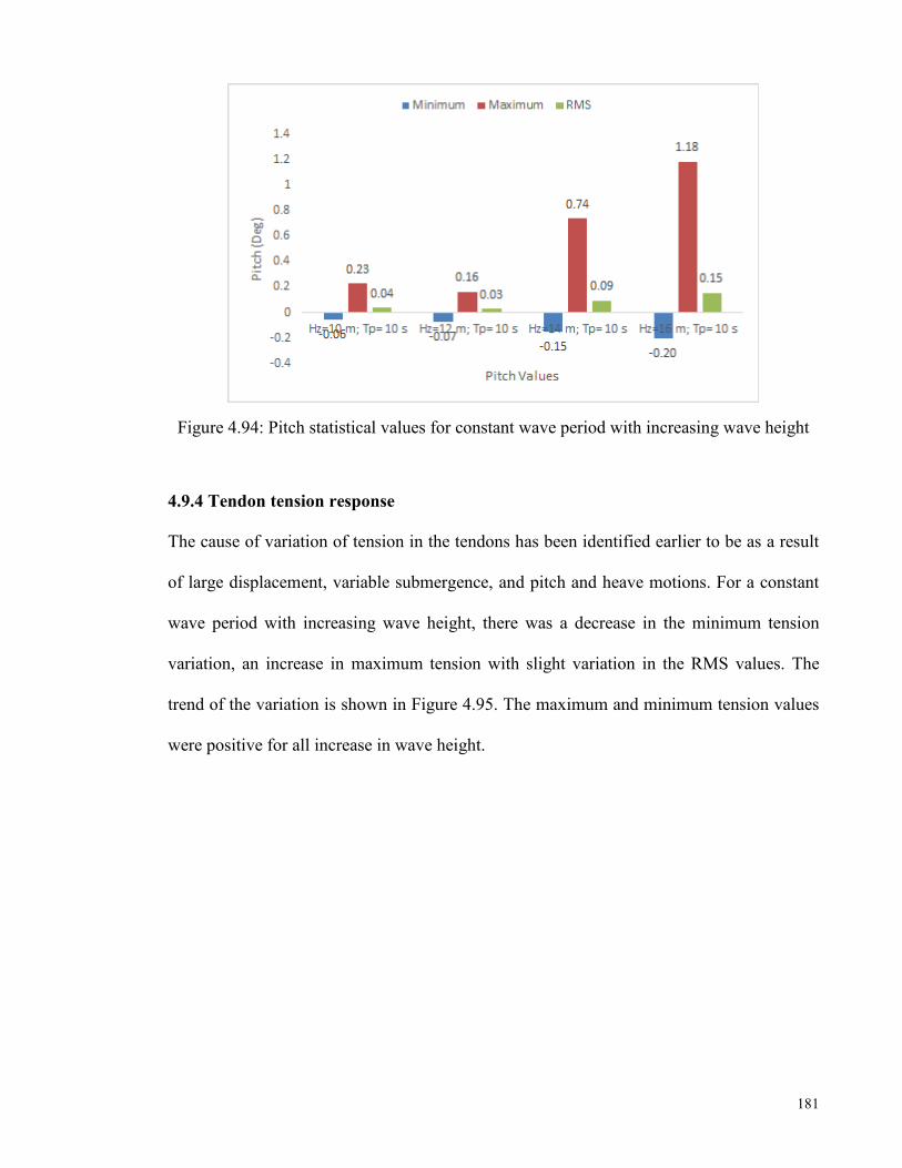
181
Figure 4.94: Pitch statistical values for constant wave period with increasing wave height
4.9.4 Tendon tension response
The cause of variation of tension in the tendons has been identified earlier to be as a result
of large displacement, variable submergence, and pitch and heave motions. For a constant
wave period with increasing wave height, there was a decrease in the minimum tension
variation, an increase in maximum tension with slight variation in the RMS values. The
trend of the variation is shown in Figure 4.95. The maximum and minimum tension values
were positive for all increase in wave height.

182
Figure 4.95: Tension statistical values for constant wave period with increasing wave height

183
CHAPTER 5: CONCLUSIONS AND RECOMMENDATIONS
5.1 Conclusion
The present research was designed to investigate the dynamic response of tension leg
platform and more specifically to examine the significance of coupling tendons with the
platform. The platform governing equation of motion was formulated from the theory of
structural engineering and idealized as rigid body approach. The tendon effect is considered
and modelled as linearized spring stiffness in uncoupled TLP while the standard finite
beam element was used to model tendons in the coupled TLP. Fluid-structure interaction is
captured by applying linearized wave theory for regular wave, wave spectrum and modified
Morison equations for the computation of the hydrodynamic forces on the structure. The
time-variant, nonlinear and response-dependent second order equation of motion was
solved numerically in time-domain.
Ocean characterization has great influence on the forces and corresponding motion of the
TLP. Previous studies have idealized ocean waves as regular, which is not true of an ocean
behaviour, while other works focused on unidirectional random wave without considering
wave directionality. This work synthesized artificial sea states for regular and irregular sea
states, hence, platform motion and tension variations in the tendons differ for regular,
unidirectional and directional random wave forces and in different load cases. The other
findings confirmed that results of simultaneous occurrence of wave, current and wind
forces predicted highest response for an ideal TLP model due to the high velocities of wind
and current for the chosen TLP and selected sea state. In addition, the effect of different sea
state parameters, consequences of removal of one tendon from the group of tendon leg, and

184
parametric study of different wave heights and wave periods on the TLP response are
investigated.
The first objective of this research was to develop and solve platform equation of motion.
This goal was achieved in Chapter Three for both coupled and uncoupled TLP models and
the developed programs are included in Appendices A and B. These programs were used to
achieve the second and third objectives which were to investigate the response of
uncoupled and coupled TLP under the action of regular, unidirectional and directional
random waves, current and wind forces. Further to this, the fourth objective on the
significance of tendon dynamics was studied in Chapter Four by including tendon
mass in the equation of motion, and applying hydrodynamic and damping forces on
the tendons. The outcome of the dynamic analysis of TLP in different load cases of regular
and irregular waves, current and wind forces was then analysed and interpreted in terms of
their magnitude, frequency of vibration and statistical measures to fulfill the fifth objective.
The following inferences were drawn from the analysis carried out for ISSC TLP in GOM
field. The motion response of the TLP was deduced to be a direct function of ocean wave
characterization, therefore, directional random wave was recommended for ocean wave
characterization. In addition, time histories, power spectral densities and statistical forms
give useful insights into platform behaviour and frequency of vibration. The vibration of
the platform predominantly occurred at the wave forcing frequency in regular wave
simulation while platform oscillation occurred at surge natural frequency in random wave
simulation, and is completely absent in regular sea wave representation. There is presence
of other cluster of peaks around wave forcing frequency. This evidence suggests that
random wave simulation represents an ideal ocean characterization and realistic TLP
behaviours.

185
The action of current drag force and low-frequency wind forces caused a steady offset and
increased dynamic behaviour in all degrees of freedom. This behaviour suggests that ocean
current, and mean and fluctuating wind forces should be included during the global motion
analysis. The maximum and minimum tension values along the tendon length differed for
different load combinations and these are reported for design of tendon leg system. The
statistical motion responses and variations in tendon tension in different load cases are
essential for decision making. Preferably, root mean square motion values are
recommended for the purpose of TLP design since the probability of occurrence of RMS
values proved that 99.7 percentage of their values lie around the mean value. The presence
of prominent peaks in pitch and tendon tension PSD confirmed nonlinearities due to
geometric nonlinearity, variable submergence and variable tendon tension. This fact
established the need for stochastic dynamic analysis of the TLP against linear static
analysis.
Lack of wave directionality in unidirectional random wave simulation led to higher motion
and tendon forces response compared to directional wave simulation. Also, the difference
between the maximum and minimum tension magnitude in directional seas was drastically
reduced when compared to unidirectional random seas. This will prove economical during
the design of strength requirement for tendons compared to regular and unidirectional sea
modelling. Time histories of platform motion was governed by a combination of surge
natural frequency of the platform as well as wave forcing frequency. As current and wind
forces act with random wave, their effect was massive on the platform motion whereas
variations in tendon forces due to these forces are not as large as motion responses.
The coupled TLP with tendon dynamics gave a true picture of platform response as
compared to an uncoupled TLP. The analysis of the TLP as an uncoupled and coupled

186
models has extended our understanding and confirmed the existing knowledge that surge
motion response was fairly predicted by the two models but heave, pitch motions and
variations in tendon tension differ significantly, hence the coupled model is recommended
for analysis purpose. There was an unequal tension distribution in the platform tendons
which could be due to result of unequal set-down, however, maximum tension variation in
the linear spring models were higher and the minimum tension variation was lower
compared to the beam elements with tendon dynamics and three out of four tendon legs
were in compression. The overall effect of an increase in wave periods at constant wave
height increased the surge, heave and pitch motion responses moderately. The increase in
wave height at a constant wave period increased the surge, heave and pitch amplitudes but
the accompanying increase in hydrodynamic damping force also damped the supposed
escalating surge response.
To conclude, numerical programs for TLP models were formulated for uncoupled and
coupled TLP models using theory of structural engineering and in an unconventional
approach. With this, a single mathematical equation of motion for the solution of a fully-
coupled TLP and tendons model that is time and cost effective, with potential to be fully
developed into a standard software was developed and used to investigate nonlinear
response of TLP to the stochastic wave and wind fields
5.2 Recommendation
The stochastic response of the tension leg platform was carried out numerically. The results
are recommendable for preliminary decision making during TLP design. Due to the
constraints of lack of laboratory facility, the following points would be recommended for
future work:
187
(1) Experimental analysis of the TLP should be carried in the standard laboratory with
realistic scale models.
(2) The effects of potential theory for the simulation of low, high and wave frequency
forces over the Morison equation should be established.
(3) The effects of vortex induced vibration on the tendons and risers and the
corresponding influence on the platform should be analysed.
(4) The effects of inclusion of riser along with tendons and platform should also be
carried out.
(5) The behaviour of the TLP in deep and ultra-deeper waters should also be accounted
for.
(6) The stability and reliability analysis of platform and tendons for the purpose of
fatigue analysis also need consideration.
(7) The numerical model formulated in FORTRAN should be expanded to include
tendon dynamics and second order wave forces.
(8) The response of the TLP using different wave and wind spectra together with
simulation of data local to the site of the study is recommended.
This research has modelled and solved a single mathematical equation of motion for a
fully-coupled TLP platform and tendons model in Abaqus/Aqua software. With this,
separate equations of motions for the platform model and the tendon leg system were
avoided as it is a norm in some of the existing hydrodynamic software for offshore
structures based on decoupled analysis such as AQWA, HOBEM, NBODY and NEPTUNE
among others. Again, set of mathematical equations for an uncoupled TLP model was
formulated in FORTRAN programming language from the existing literatures.

188
Another contribution of this work is that Abaqus finite element tool that was not
originally designed for the solution of offshore platforms was adapted for the platform
model discretization. This was integrated with Abaqus/Aqua module for the application of
hydrodynamic and aerodynamic loadings on the platform. The result of this approach is
that offshore problem with high-level complexities is solved using knowledge of Civil
Engineering.
By this research and with the validation that has been carried out, knowledge
dissemination is enhanced and is made available to any researcher that want to go into
analysis of offshore platform since the specialized software are expensive and require
extensive time to comprehend. The numerical models have several practical applications
such as assessment of different load cases for decision making. Various forms of
environmental forces that the model was equipped with are regular wave, unidirectional
and directional random waves, current and wind forces.
The analysis of the TLP as uncoupled and coupled model has extended our
understanding to know that surge motion response can be taken to be fairly predicted by the
two models but heave, pitch motions and variations in tendon tension differ significantly,
hence coupled model is recommended. The findings from the ocean characterization
suggest that ocean idealization influence forces and corresponding motions of the platform,
however directional random wave idealization is recommended for a realistic sea. Taken
together, TLP response in the combined action of wave, current and wind forces produce
the largest response and simulating the model for all these loadings are recommended.
Finally, the numerical models have proved to be valuable as a research tool and have
potential to be developed as full-fledged software.
189
REFERENCES
Abaqus, C. (2011). Abaqus analysis user’s manual Velizy-Villacoublay, France: Dassault Systemes.
Abou-Rayan, A., Seleemah, A., & El-Gamal, A. R. (2012). Response of square tension leg platforms to hydrodynamic forces. Ocean Systems Engineering, 2(2), 115-135.
Abou-rayan, A. M., & Hussein, O. S. (2014). Dynamic Reponses of Square TLP's to Random Wave Forces. International Journal of Civil Engineering, 3(2), 103 -110.
Adamiec-Wojcik, I., Brzozowska, L., & Drag, L. (2015). An analysis of dynamics of risers during vessel motion by means of the rigid finite element method. Ocean Engineering, 106, 102-114. doi:10.1016/j.oceaneng.2015.06.053
Adrezin, R., Bar-Avi, P., & Benaroya, H. (1996). Dynamic Response of Compliant Offshore Structures- Review. Journal of Aerospace Engineering, 9.
Adrezin, R., & Benaroya, H. (1999a). Non-linear stochastic dynamics of tension leg platforms. Journal of Sound and Vibration, 220(1), 27-65. doi: 10.1006/jsvi.1998.1915
Adrezin, R., & Benaroya, H. (1999b). Response of a tension leg platform to stochastic wave forces. Probabilistic Engineering Mechanics, 14(1-2), 3-17. doi: 10.1016/S0266-8920(98)00012-5
Aguiar, L. L., Almeida, C. A., & Paulino, G. H. (2014). A three-dimensional multilayered pipe beam element: Nonlinear analysis. Computers & Structures, 138, 142-161. doi:10.1016/j.compstruc.2013.09.005
Ahmad, S. (1996). Stochastic TLP response under long crested random sea. Computers & Structures, 61(6), 975-993. doi:10.1016/0045-7949(96)00188-5
Ahmad, S., Islam, N., & Ali, A. (1997). Wind-induced response of a tension leg platform. Journal of Wind Engineering and Industrial Aerodynamics, 72(1-3), 225-240. doi:10.1016/S0167-6105(97)00238-9
Amanullah, M., Siddiqui, N. A., Umar, A., & Abbas, H. (2002). Fatigue reliability analysis of welded joints of a TLP tether system. Steel & Composite Structures, 2(5), 331-354.

190
American Petroleum Institute. (1996). Recommended practice for design analysis of station-keeping systems for floating structure. API-RP2SK. Washington DC: American Petroleum Institute.
American Petroleum Institute. (2001). Recommended Practice for Planning, Designing, and Constructing Floating Production Systems API Recommended Practice 2FPS: API Publishing Services, 1220 L Street, N.W., Washington, D.C, 20005.
Ardakani, H. A., & Ketabdari, M. J. (2007). Experimental study on the response behaviour of seastar mini tension leg platform against random water waves. Proceedings of the 26th International Conference on Offshore Mechanics and Arctic Engineering, Vol 1, 767-776.
Astrup, O., Nestegård, A., Ronæss, M., & Sødahl, N. (2001). Coupled analysis strategies for deepwater spar platforms. Paper presented at the The Eleventh International Offshore and Polar Engineering Conference.
Bachynski, E. E., & Moan, T. (2012). Design considerations for tension leg platform wind turbines. Marine Structures, 29(1), 89-114. doi:10.1016/j.marstruc.2012.09.001
Bahtui, A., Alfano, G., Bahai, H., & Hosseini-Kordkheili, S. A. (2010). On the multi-scale computation of un-bonded flexible risers. Engineering Structures, 32(8), 2287-2299. doi:10.1016/j.engstruct.2010.04.003
Bar-Avi, P. (1999). Nonlinear Dynamic Response of a Tension Leg Platform. Journal of Offshore Mechanics and Arctic Engineering, 121(4), 219-226. doi:10.1115/1.2829571
Barranco-Cicilia, F., Lima, E. C. P., & Sagrilo, L. V. S. (2008). Reliability-based design criterion for TLP tendons. Applied Ocean Research, 30(1), 54-61. doi:10.1016/j.apor.2008.05.001
Bathe, K.-J. (1982). Finite Element Procedures in Engineering Analysis: Prentice-Hall, Inc., Englewood Cliffs, New Jersey 07632.
Benfratello, S., Di Paola, M., & Spanos, P. D. (1998). Stochastic Response of MDOF Wind-Excited Structures by means of Volterra series approach. Journal of Wind Engineering and Industrial Aerodynamics, 74—76.
191
Bhattacharyya, S. K., Sreekumar, S., & Idichandy, V. G. (2003). Coupled dynamics of SeaStar mini tension leg platform. Ocean Engineering, 30(6), 709-737. doi:10.1016/S0029-8018(02)00061-6
Bisht, R. S., & Jain, A. K. (1997). Wind and wave induced behaviour of offshore guyed tower platforms. Ocean Engineering, 25(7), 501-519.
Borgman, L. E. (1967). Ocean wave simulation for engineering design Wave research project. Corps of Engineers, U.S Army.: Contract DA-49-055-CIV-ENG-64-4 Coastal Engineering research center.
Caire, M., & Schiller, R. (2012). The effect of coupled dynamic analysis of floater motions on the mooring and riser system response of an FPSO. Marine Systems & Ocean Technology, 7(2), 95-106.
Chakrabarti, S. (2005). Handbook of Offshore Engineering (2005 ed. Vol. 1). Elsevier, The Boulevard, Langford Lane, Kidlington, Oxford OX5 IGB, UK.
Chakrabarti, S. K. (1971). Discussion of Dynamics of Single Point Mooring in Deep Water by John H. Nath and Michael P. Felix. Journal of the Waterways, Harbors and Coastal Engineering Division, 97(3), 588-590.
Chakrabarti, S. K. (1987). Hydrodynamics of offshore structures: Computational Mechanics.
Chakrabarti, S. K. (2008). Challenges for a Total System Analysis on Deepwater Flaoting Systems. The Open Mechanics Journal, 2, 28-46.
Chandak, N. R., & Chandrasekaran, S. (2010). Structural Response of Triangular Tension Leg Platform Using Dynamic Morison Equation. Iscm Ii and Epmesc Xii, Pts 1 and 2, 1233, 1483-1488. doi:10.1063/1.3452127
Chandrasekaran, S., Chandak, N. R., & Anupam, G. (2006). Stability analysis of TLP tethers. Ocean Engineering, 33(3-4), 471-482. doi:10.1016/j.oceaneng.2005.04.015
Chandrasekaran, S., & Gaurav. (2008). Offshore triangular tension leg platform earthquake motion analysis under distinctly high sea waves. Ships and Offshore Structures, 3(3), 173 - 184. doi:10.1080/17445300802051681

192
Chandrasekaran, S., & Jain, A. K. (2002a). Dynamic behaviour of square and triangular offshore tension leg platforms under regular wave loads. Ocean Engineering, 29(3), 279-313. doi:10.1016/S0029-8018(00)00076-7
Chandrasekaran, S., & Jain, A. K. (2002b). Triangular Configuration Tension Leg Platform behaviour under random sea wave loads. Ocean Engineering, 29(15), 1895-1928. doi:10.1016/S0029-8018(01)00111-1
Chandrasekaran, S., Jain, A. K., & Chandak, N. R. (2004). Influence of Hydrodynamic Coefficients in the Response Behavior of Triangular TLPs in Regular Waves. Ocean Engineering, 31, 2319–2342.
Chandrasekaran, S., Jain, A. K., & Chandak, N. R. (2006). Seismic analysis of offshore triangular tension leg platforms. International Journal of Structural Stability and Dynamics, 6(1), 97-120. doi:10.1142/S0219455406001848
Chandrasekaran, S., Jain, A. K., Gupta, A., & Srivastava, A. (2007). Response behavior of triangular tension leg platforms under impact loading. Ocean Engineering, 34, 45-53. doi:10.1016/j.oceaneng.2006.01.002
Chapra, S. C., & Canale, R. P. (2012). Numerical methods for engineers (Vol. 2): McGraw-Hill New York.
Chatterjee, P. C., Das, P. K., & Faulkner, D. (1996). A Hydro-structural Analysis Program for TLPs. Ocean Engineering, 24(4), 313-334.
Chen, J. M., Kong, X. Y., & Sun, Y. (2013). Hydrodynamic Responses Analysis for Tension Leg Platform. In X. H. Liu, K. F. Zhang, & M. Z. Li (Eds.), Manufacturing Process and Equipment, Pts 1-4 (Vol. 694-697, pp. 27-30). Stafa-Zurich: Trans Tech Publications Ltd.
Chernetsov, V. A., & Karlinsky, S. L. (2006). Ice-resistant spar-type platform for middle sea depth. Proceedings of the Sixteenth (2006) International Offshore and Polar Engineering Conference, Vol 1, 614-619.
Chitrapu, A., & Ertekin, R. (1992). Effect of nonlinear drag forces on the low-and high-frequency response of floating platforms. Paper presented at the 11th Intl Conf on Offshore Mechanics & Arctic Engng, Calgary, Canada.
193
Chitrapu, A., & Ertekin, R. (1993). Nonlinear Effects in Floating Platform Response Using Time-Domain Simulation Methods. Paper presented at the 12th Intl Conf on Offshore Mechanics & Arctic Engng, Glasgow, UK. .
Chitrapu, A. S., & Ertekin, R. C. (1995). Time-Domain Simulation of Large-Amplitude Response of Floating Platforms. Ocean Engineering, 22(4), 367-385. doi:10.1016/0029-8018(94)00013-W
Chitrapu, A. S., Ertekin, R. C., & Paulling, J. R. (1993). Viscous drift forces in regular and irregular waves. Ocean Engineering, 20(1), 33-55. doi:10.1016/0029-8018(93)90045-J
Clough, R. W., & Penzien, J. (1993). Dynamics of structures. 1993. Copyright of Applied Mechanics & Materials.
Correa, F. N., Jacob, B. P., & Mansur, W. J. (2010). Formulation of an efficient hybrid time–frequency domain solution procedure for linear structural dynamic problems. Computers & Structures, 88(5), 331-346.
Correa, F. N., Senra, S. F., Jacob, B. P., Masetti, I. Q., & Mourelle, M. M. (2002). Towards the integration of analysis design of mooring systems risers, Parts I & II: Studies on a Dicas System. Paper presented at the Proceedings of Offshore Mechanics Arctic Engineering Conference.
D'Souza, R., Aggarwal, R., & Basu, S. (2013). The Tension Leg Platform-A Retrospective. Paper presented at the Proceedings of the 18th SNAME Offshore Symposium,“Engineering the Future: The Arctic and Beyond,” Houston, Texas.
Dassault, S. (2009). Abaqus Documentation Version 6.9. United States of America: Dassault System, Simulia Corp, Providence, RI, USA.
Dawson, T. H. (1983). Offshore structural engineering (illustrated ed.). The University of Michigan: Prentice-Hall.
Demirbilek, Z. (1990). Design Formulas for Offset, Set down and Tether Loads of a Tension Leg Platform (TLP). Ocean Engineering, 17(5), 517-523. doi:10.1016/0029-8018(90)90042-5
El-gamal, A. R., Essa, A., & Ismail, A. (2014). Effect of Tethers Tension Force on the Behaviour of Traiangular Tension Leg Platform. American Journal of Civil Engineering and Architecture, 2(3), 107 - 114. doi:10.12691/ajcea-2-3-3
194
Elshafey, A. A., Haddara, M. R., & Marzouk, H. (2009). Dynamic response of offshore jacket structures under random loads. Marine Structures, 22(3), 504-521. doi:http://dx.doi.org/10.1016/j.marstruc.2009.01.001
Gadagi, M. M., & Benaroya, H. (2006). Dynamic response of an axially loaded tendon of a tension leg platform. Journal of Sound and Vibration, 293(1-2), 38-58. doi:10.1016/j.jsv.2005.09.027
Gao, Y. W., Li, C., & Cheng, X. (2013). Performance Research on Tension Leg Platform of Floating Offshore Wind turbine. In A. Wang, L. K. Che, R. Dong, & G. Zhao (Eds.), Applied Energy Technology, Pts 1 and 2 (Vol. 724-725, pp. 645-648). Stafa-Zurich: Trans Tech Publications Ltd.
Garrett, D. L. (2005). Coupled analysis of floating production systems. Ocean Engineering, 32, 802 - 816. doi:10.1016/j.oceaneng.2004.10.010
Gie, T. S., & de Boom, W. (1981). The wave induced motions of a tension leg platform in deep water. Paper presented at the Offshore Technology Conference.
Giron, A. R. C., Correa, F. N., & Jacob, B. P. (2014). An Evaluation of the Semi-Coupled Scheme for the Analysis of Floating Production Systems. Paper presented at the Proceedings of the ASME 2014 33rd International Conference on Ocean, Offshore and Artic Engineering, OMAE2014, San Francisco, California, USA.
Goda, Y. (1970). Numerical experiments on wave statistics with spectral simulation. Report of the Port and Harbour Research Institute, 9(3), 3-57.
Guarga, F., Castells, M., Bosch, R., & Casals, P. (2014). Theorical and descriptive analysis of the wave energy in the “Barcelona World Race”. Journal of Maritime Research, 11(2), 41-51.
Han, S. M., & Benaroya, H. (2002). Comparison of linear and nonlinear responses of a compliant tower to random wave forces. Chaos, Solitons and Fractals. doi:14 269-291.S0960-0779 (01) 00232-6
Hogben, N., & Standing, R. (1974). Wave loads on large bodies. Paper presented at the Proceedings of the International Symposium on the Dynamics of Marine Vehicles and Structures in Waves.
Horton, E. E., Brewer, J. H., Silcox, W. H., & Hudson, T. A. (1976). "Means and methods for anchoring an offshore tension leg platform". (934,528). US.
195
Islam, A., Jameel, M., Jumaat, M. Z., Shirazi, S. M., & Salman, F. A. (2012). Review of offshore energy in Malaysia and floating Spar platform for sustainable exploration. Renewable & Sustainable Energy Reviews, 16(8), 6268-6284. doi:10.1016/j.rser.2012.07.012
Islam, A. B. M. S., Jameel, M., Ahmad, S., Jumaat, M. Z., & Kurian, V. J. (2013). Structural Behaviour of Fully Coupled Spar-Mooring System under Extreme Wave Loading. Journal of Civil Engineering and Management, 19, S69-S77. doi:10.3846/13923730.2013.801899
Islam, A. B. M. S., Jameel, M., & Jumaat, M. Z. (2012). Oil and Gas Energy Potential at Malaysian Seabed and Spar Platform for Deepwater Installation. International Journal of Green Energy, 9(2), 111-120. doi:10.1080/15435075.2011.621493
Islam, A. B. M. S., Soeb, M. R., & Jumaat, M. Z. B. (2016). Floating spar platform as an ultra-deepwater structure in oil and gas exploration. Ships and Offshore Structures, 1-14. doi:10.1080/17445302.2015.1112179
Jain, A. K. (1997). Nonlinear coupled response of offshore tension leg platforms to regular wave forces. Ocean Engineering, 24(7), 577-592. doi:10.1016/0029-8018(95)00059-3
Jameel, M., Ahmad, S., Islam, A., & Jumaat, M. Z. (2013). Non-linear dynamic analysis of coupled Spar platform. Journal of Civil Engineering and Management, 19(4), 476-491. doi:10.3846/13923730.2013.768546
Jameel, M., Ahmad, S., Islam, A., & Jumaat, M. Z. (2014). Wind Induced Nonlinear Response of Coupled SPAR Platform. Paper presented at the Proceedings of the ASME 2014 33rd International Conference on Ocean, Offshore and Artic Engineering, OMAE2014, San Francisco, California, USA.
Jameel, M., Oyejobi, D. O., Siddiqui, N. A., & Ramli Sulong, N. H. (2016). Nonlinear dynamic response of tension leg platform under environmental loads. KSCE Journal of Civil Engineering, 1-9. doi:10.1007/s12205-016-1240-8
Jayalekshmi, R., Sundaravadivelu, R., & Idichandy, V. G. (2009). Hull-tether-riser dynamics of deep water tension leg platforms. Fluid Structure Interaction V, 105, 215-223. doi:10.2495/Fsi090201
Jayalekshmi, R., Sundaravadivelu, R., & Idichandy, V. G. (2010). Dynamic Analysis of Deep Water Tension Leg Platforms Under Random Waves. Journal of Offshore

196
Mechanics and Arctic Engineering-Transactions of the Asme, 132(4), 4. doi:10.1115/1.4001432
Jefferys, E. R., & Patel, M. H. (1982). Dynamic Analysis Models of Tension Leg Platforms. Journal of Energy Resources Technology, 104(3), 217-223. doi:10.1115/1.3230406
Jensen, J. J., & Capul, J. (2006). Extreme response predictions for jack-up units in second order stochastic waves by FORM. Probabilistic Engineering Mechanics, 21(4), 330-337.
Jia, J. (2008). An efficient nonlinear dynamic approach for calculating wave induced fatigue damage of offshore structures and its industrial applications for lifetime extension. Applied Ocean Research, 30(3), 189-198.
Joseph, A., Mangal, L., & George, P. S. (2009). Coupled Dynamic Response of a Three- Column Mini TLP. Journal of Naval Architecture and Marine Engineering, 6, 52 - 61. doi:10.3329/jname.v6i2.2789
Kang, W.-H., Zhang, C., & Yu, J.-X. (2016). Stochastic extreme motion analysis of jack-up responses during wet towing. Ocean Engineering, 111, 56-66.
Kappos, A. J. (2002). Dynamic Loading and Design of Structures. London: Spons Press.
Kareem, A., & Li, Y. S. (1993). Wind-Excited Surge Response of Tension-Leg Platform - Frequency-Domain Approach. Journal of Engineering Mechanics-Asce, 119(1), 161-183. doi:10.1061/(Asce)0733-9399(1993)119:1(161)
Karlinsky, S. L., & Kuteynikov, M. A. (2008). Damage Stability of Tension Leg Platform in Ice Environment. Paper presented at the 8th International Conference on the stability of ships and Ocean Vehicles. Escuela Tecnica Superior de Ingenieros Navales.
Khan, R. A., Siddiqui, N. A., Naqvi, S. Q. A., & Ahmad, S. (2006). Reliability analysis of TLP tethers under impulsive loading. Reliability Engineering & System Safety, 91(1), 73-83. doi:10.1016/j.ress.2004.11.010
Kim, C. H., Lee, C. H., & Goo, J. S. (2007). A dynamic response analysis of tension leg platforms including hydrodynamic interaction in regular waves. Ocean Engineering, 34(11-12), 1680-1689. doi:10.1016/j.oceaneng.2006.10.011

197
Kurian, V. J., Gasim, M. A., Narayanan, S. P., & Kalaikumar, V. (2008). Parametric studies subjected to random waves. Paper presented at the ICCBT 2008, Kuala Lumpur, Malaysia.
Le, C. H., Ding, H. Y., & Zhang, P. Y. (2014). Dynamic response analysis of a floating mooring system. Journal of Ocean University of China, 13(3), 381-389. doi:10.1007/s11802-014-2023-9
Lee, H. H., & Wang, P. W. (2000). Analytical solution on the surge motion of tension-leg twin platform structural systems. Ocean Engineering, 27(4), 393-415.
Lei, S., Zhang, W. S., Lin, J. H., Yue, Q. J., Kennedy, D., & Williams, F. W. (2014). Frequency domain response of a parametrically excited riser under random wave forces. Journal of Sound and Vibration, 333(2), 485-498. doi:10.1016/j.jsv.2013.09.025
Li, Y. S., & Kareem, A. (1990). Stochastic Response of Tension Leg Platforms to Wind and Wave Fields. Journal of Wind Engineering and Industrial Aerodynamics, 36(1-3), 915-926.
Liu, W. M. (2014). Research on Time-domain Dynamic Response of Tension Leg Platform in Regular Wave. Applied Mechanics, Materials and Manufacturing Iv, 670-671, 801-804. doi:10.4028/www.scientific.net/AMM.670-671.801
Low, Y. M. (2009). Frequency domain analysis of a tension leg platform with statistical linearization of the tendon restoring forces. Marine Structures, 22(3), 480-503. doi:10.1016/j.marstruc.2009.01.002
Low, Y. M., & Langley, R. S. (2006). Time and frequency domain coupled analysis of deepwater floating production systems. Applied Ocean Research, 28(6), 371-385. doi:10.1016/j.apor.2007.05.002
Lyons, G. J., & Patel, M. H. (1984). Comparisons of Theory With Model Test Data for Tensioned Buoyant Platforms. Journal of Energy Resources Technology, 106(4), 426-436. doi:10.1115/1.3231102
Mao, D., Zhong, C., Zhang, L., & Chu, G. (2015). Dynamic response of offshore jacket platform including foundation degradation under cyclic loadings. Ocean Engineering, 100, 35-45.
198
Masciola, M., & Nahon, M. (2008). Modeling and Simulation of a Tension Leg Platform. Proceedings of the Eighteenth (2008) International Offshore and Polar Engineering Conference, Vol 1, 84-91.
Masciola, M., Nahon, M., & Driscoll, F. (2013). Preliminary Assessment of the Importance of Platform-Tendon Coupling in a Tension Leg Platform. Journal of Offshore Mechanics and Arctic Engineering-Transactions of the Asme, 135(3), 11. doi:10.1115/1.4023795
Mekha, B. B., Johson, C. P., & Roesset, J. M. (1996). Implications of Tendon Modeling on Nonlinear Response of TLP. Journal of Structural Engineering, 122, 142 - 149.
Mohd Zaki, N. I., Abu Hussain, M. K., & Najafian, G. (2014). Extreme structural response values from various methods of simulating wave kinematics. Ships and Offshore Structures. doi:10.1080/17445302.2014.987947
Morgan, J. R. (1983). Dynamic analysis of tension-leg platforms: ; Texas A and M Universty College Station, Texas.
Muhittin, S., & Oguz, Y. (2003). Hydrodynamic Design of a TLP type Offloading Platform. Ocean Engineering, 30, 1269–1282.
Naess, A., Gaidai, O., & Teigen, P. S. (2007). Extreme response prediction for nonlinear floating offshore structures by Monte Carlo simulation. Applied Ocean Research, 29(4), 221-230. doi:10.1016/j.apor.2007.12.001
Nallayarasu, S. (2008). Offshore Structures (Analysis and Design). Department of Ocean Engineering, Indian Institute of Technology Madras, Chennais-600036. Indian.
Natvig, B. J., & Johnsen, O. (2000). Coupled dynamics of tether and platform for a North Sea wellhead TLP. Paper presented at the International Society of Offshore and Polar Engineers Conf (ISOPE 2000), .
Ng, C. Y., Kurian, V. J., & Liew, M. S. (2014). Dynamic responses of classic spar platform: Short crested waves vs long crested waves. Applied Mechanics and Materials, 567, 235-240. doi:10.4028/www.scientific.net/AMM.567.235
Nwogu, O., & Irani, M. (1990). Numerical prediction of higher order wave induced loads on tethered platforms. Paper presented at the The First ISOPE European Offshore Mechanics Symposium.
199
Offshore Magazine. (2010). 2010 Worldwide Survey of TLPs, TLWPs. Lindsey Wilhot and Chad Supan of Mustang Engineering.
Ormberg, H., Baarholm, R., & Stansberg, C. T. (2003). Time-domain coupled analysis of deepwater TLP, and verification against model tests. Paper presented at the The Thirteenth International Offshore and Polar Engineering Conference.
Ormberg, H., & Larsen, K. (1998). Coupled analysis of floater motion and mooring dynamics for a turret-moored ship. Applied Ocean Research, 20(1), 55-67.
Paulling, J., & Webster, W. C. (1986). A consistent, large-amplitude analysis of the coupled response of a TLP and tendon system. Paper presented at the Proceedings of the Fifth International Symposium on Offshore Mechanics and Arctic Engineering, Tokyo.
Refat, H. M., & El-gamal, A. R. (2014). Influence of the Density of Water on the Dynamic Behaviour of Square Tension Lag Platform. American Journal of Civil Engineering and Architecture, 2(4), 122 - 129. doi:10.12691/ajcea-2-4-1
Rijken, O., & Leverette, S. (2007). Tension Leg Platform response to earthquake in Gulf of Mexico. Proceedings of the Seventeenth (2007) International Offshore and Polar Engineering Conference, Vol 1- 4, Proceedings, 190-193.
Rudman, M., & Cleary, P. W. (2013). Rogue wave impact on a tension leg platform: The effect of wave incidence angle and mooring line tension. Ocean Engineering, 61, 123-138. doi:10.1016/j.oceaneng.2013.01.006
Salpukas, A. (1994). Oil companies drawn to the deep. The New York Times December, 7, D1.
Sannasiraj, S., Sundar, V., & Sundaravadivelu, R. (1995). The hydrodynamic behaviour of long floating structures in directional seas. Applied Ocean Research, 17(4), 233-243.
Sen, D. (2002). Time-domain simulation of large structures in nonlinear waves. Paper presented at the Proceedings of 21st International Conference on Offshore Mechanics Arctic Engineering, OMAE 2002-28033, Oslo, Norway.
Senjanovic, I., Tomic, M., & Hadzic, N. (2013). Formulation of consistent nonlinear restoring stiffness for dynamic analysis of tension leg platform and its influence on response. Marine Structures, 30, 1-32. doi:10.1016/j.marstruc.2012.10.007

200
Senjanovic, I., Tomic, M., & Rudan, S. (2013). Investigation of nonlinear restoring stiffness in dynamic analysis of tension leg platforms. Engineering Structures, 56, 117-125. doi:10.1016/j.engstruct.2013.04.020
Shehata, E., & Raheem, A. (2013). Nonlinear response of fixed jacket offshore platforn under structural and wave loads. Coupled Systems Mechanics, 2(1), 111 -126.
Siddiqui, N., & Ahmad, S. (2001). Fatigue and fracture reliability of TLP tethers under random loading. Marine Structures, 14(3), 331-352.
Siddiqui, N. A., & Ahmad, S. (2003). Dynamic behaviour of tension leg platform under impulsive loading. Defence Science Journal, 53(2), 205-210.
Simiu, E., & Leigh, S. D. (1984). Turbulent Wind and Tension Leg Platform Surge. Journal of Structural Engineering-Asce, 110(4), 785-802.
Spanos, P. D., & Agarwal, V. K. (1984). Response of a Simple Tension Leg Platform Model to Wave-Forces Calculated at Displaced Position. Journal of Energy Resources Technology-Transactions of the Asme, 106(4), 437-443.
Tabeshpour, M. R., Golafshani, A. A., & Seif, M. S. (2006). Second-order perturbation added mass fluctuation on vertical vibration of tension leg platforms. Marine Structures, 19(4), 271-283. doi:http://dx.doi.org/10.1016/j.marstruc.2007.02.001
Tabeshpour, M. R., & Shoghi, R. (2014). Nonlinear dynamic analysis of TLP surge motion using homotopy perturbation method. Ships and Offshore Structures, 9(6), 569-577. doi:10.1080/17445302.2014.912045
Taylor, R. E., & Jefferys, E. R. (1986). Variability of Hydrodynamic Load Predictions for a Tension Leg Platform. Ocean Engineering, 13(5), 449-490.
Veritas, B. (2012). Rules for the classification of tension leg platform (TLP). In V. Bureau (Ed.).
Veritas, D. N. (2007). Environmental conditions and environmental loads. Retrieved from Veritas-veien 1, NO -1322 Hovik, Norway:
Veritas, D. N. (2008). Structural Design of TLPS (LRFD METHOD). Veritasveien 1, NO- 1322 Hovik, Norway.
201
Vickery, P. J. (1995). Wind-Induced Response of Tension Leg Platform - Theory and Experiment. Journal of Structural Engineering-Asce, 121(4), 651-663. doi:10.1061/(Asce)0733-9445(1995)121:4(651)
Vlahos, G., Cassidy, M. J., & Martin, C. M. (2008). Experimental investigation of the system behaviour of a model three-legged jack-up on clay. Applied Ocean Research, 30(4), 323-337.
Wheeler, J. (1969). Methods for calculating forces produced by irregular waves. Paper presented at the Offshore Technology Conference.
Wilson, J. F. (2003). Dynamics of Offshore Structures. New Jersey: John Wiley & Sons, Inc.
Yang, M., Teng, B., Ning, D., & Shi, Z. (2012). Coupled dynamic analysis for wave interaction with a truss spar and its mooring line/riser system in time domain. Ocean Engineering, 39, 72-87. doi:10.1016/j.oceaneng.2011.11.002
Yang, M. D., Teng, B., Xiao, L. F., Ning, D. Z., Shi, Z. M., & Qu, Y. (2014). Full time-domain nonlinear coupled dynamic analysis of a truss spar and its mooring/riser system in irregular wave. Science China-Physics Mechanics & Astronomy, 57(1), 152-165. doi:10.1007/s11433-013-5273-4
Yilmaz, O., & Incecik, A. (1996a). Hydrodynamic design of moored floating platforms. Marine Structures, 9(5), 545-575.
Yilmaz, O., & Incecik, A. (1996b). Hydrodynamic Design of Moored Floating Platforms. Marine Structures, 9, 545 – 575. doi:0951-8339 (95) 00011-9
Yongjun, J., Jiemin, Z., & Qingyong, Z. (2008). Short crested wave-current forces around a large verical circular cylinder. European Journal of Mechanics B/Fluids, 27, 346 - 360. doi:10.1016/j.euromechflu.2007.08.001
Yoshida, K., Ozaki, M., & Oka, N. (1984). Structural Response Analysis of Tension Leg Platforms. Journal of Energy Resources Technology, 106(1), 10-17. doi:10.1115/1.3231005
Zaheer, M. M., & Islam, N. (2012). Stochastic response of a double hinged articulated leg platform under wind and waves. Journal of Wind Engineering and Industrial Aerodynamics, 111, 53-60. doi:10.1016/j.jweia.2012.08.005

202
Zeng, X. H., Liu, J. Y., Liu, Y., & Wu, Y. X. (2007). Parametric studies of tension leg platform with large amplitude motions. Proceedings of the Seventeenth (2007) International Offshore and Polar Engineering Conference, Vol 1- 4, Proceedings, 202-209.
Zeng, X. H., Shen, X. P., & Wu, Y. X. (2007). Governing equations and numerical solutions of tension leg platform with finite amplitude motion. Applied Mathematics and Mechanics-English Edition, 28(1), 37-49. doi:10.1007/s10483-007-0105-1
Zou, J. (2003). TLP Hull/ Tendon/Riser Coupled Dynamic Analysis in Deepwater. Paper presented at the Proceedings of the Thirteeth (2003) International Offshore and Polar Engineering Conference, Honolulu, Hawaii, USA.

203
LIST OF PUBLICATIONS AND PAPERS PRESENTED
1) M. Jameel, D.O. Oyejobi, N.A. Siddiqui & N.H Ramli Sulong (2016) Nonlinear
Dynamic Response of Tension Leg Platform under Environmental Loads, KSCE
Journal of Civil Engineering, doi 10.1007/s12205-016-1240-8, pISSN 1226-7988,
eISSN 1976-3808
2) D.O. Oyejobi, M. Jameel, & N.H Ramli Sulong (2016) Nonlinear Response of
Tension Leg Platform to Wave, Current and Wind Forces, International Journal of
Civil Engineering, (IJCE), doi: 10.1007/s40999-016-0030-5
3) D.O. Oyejobi, M. Jameel, & N.H Ramli Sulong (2016) Stochastic response of intact
and a removed tendon tension leg platform to random wave and current forces, The
Arabian Journal of Science and Engineering, (AJSE), DOI: 10.1007/s13369-016-
2282-4.
4) D.O. Oyejobi, M. Jameel, & N.H Ramli Sulong (2016) Dynamic behaviour of
tension leg platform in short-crested directional seas, ICCOEE2016, International
Conference on Civil, Offshore & Environmental Engineering, 15 – 17 August,
Kuala Lumpur, Malaysia.

204
APPENDIX
Appendix A
Program TLP common/instime/t,eta common/indata1/rmtlp,rx,ry,rz common/indata2/t0,fb,draft,cl,em,cc,dc,diah,diav,rho,vcg common/wavedata/wh,wp,cd,ci,g,d common/currentdata/vci,vcf common/windata/cdsea,ca,rhoa,akv,proarea,zref,wvref common/winflucdata/fs,fm,beta,cy,alu,wb common/impulse/impu,dura,ts,rimpul common/glob/rk,iflag,jflag,kflag,nnw,aeta,rki,w common/urand/uprime dimension rs(10,10),rm(10,10),c(10,10),f(10) dimension u(10),v(10),a(10),sumsq(10),rms(10) real aeta(200),rki(200),w(200),an(100),ueq(100),snn(200) real phasang(100),u_array(100),uprime(100),ff(100) !### integer nnw,nwind,iflag,jflag,kflag character cnum character *20 input character *20 output write(*,*) 'enter the name of data file' read(*,'(a)') input write(*,*) 'enter the name of result files (no file extension)' read(*,'(a)') output open(7,file=input) open(8,file=trim(output)//'.txt') open(9,file='eta'//trim(output)//'.txt') !dump t,eta open(11,file='rwav'//trim(output)//'.txt') !rwav_t0 open(13,file='wind'//trim(output)//'.txt') !from calcwind !### ! Data read(7,*)rmtlp ; read(7,*)vci ; read(7,*)vcf ; read(7,*)rx read(7,*)ry ; read(7,*)rz ; read(7,*)totalt0 ; read(7,*)fb read(7,*)d ; read(7,*)draft ; read(7,*)em ; read(7,*)cc read(7,*)dc ; read(7,*)diav ; read(7,*)diah ; read(7,*)rho read(7,*)ci ; read(7,*)cdsea ; read(7,*)ca ; read(7,*)rhoa read(7,*)akv ; read(7,*)proarea ; read(7,*)zref ; read(7,*)wvref read(7,*)za ; read(7,*)yac ; read(7,*)fs ; read(7,*)fm read(7,*)beta ; read(7,*)cy ; read(7,*)alu ; read(7,*)wb

205
if (jflag .ne. 0) then do i=1,8 write(cnum,'(i1)') i ! internal write open(20+i,file='member'// cnum //'.txt') end do end if nnw=0 if (iflag .ne. 0) then read(7,*) nnw read(7,*) kflag end if ! clean up keyboard entry logic and prompts write(*,*) 'For wind enter 0 for none, 1 for mean, 2 for fluctuating or 3 for both' read(*,*) in if (in < 0 .or. in > 3) then write(*,*) 'bad selection' stop end if write(*,*) 'For missing tether enter 0 for no, 1 for yes' read(*,*) imiss if (imiss < 0 .or. imiss > 1) then write(*,*) 'bad selection' stop end if write(*,*) 'For impulse enter 0 for none, 1 for rectangular' write(*,*) '2 for sinusoidal, 3 for halftriangle, 4 for triangle' read(*,*) impu if (impu < 0 .or. impu > 4) then write(*,*) 'bad selection' stop end if if (impu > 0) then write(*,*) 'Impulse Parameters' write(*,*) 'Start time?' read(*,*) ts write(*,*) 'Duration?' read(*,*) dura write(*,*) 'Size?' read(*,*) rimpul end if x=0 y=0

206
t0=totalt0/4.0 vcg= cgfo+draft cl=d-draft g=9.81 pi=4.0*atan(1.0) omega=2.0*pi/wp rk=omega**2/g !deep water, skip newton approx wavelength = 2.0*pi/rk write(*,'(a,f10.2)')'wavelength (m)=',wavelength if( diav/wavelength .le. 0.2 .and. diah/wavelength .le. 0.2) then write(*,*)'Morrison Applicable' else write(*,*)'Morrison not Applicable' end if if (in > 0) then call calcwind(in,za,yac,nwind,an,ueq,wv,ff) !calc fixed values once ### end if !uncomment next statement to have new random #s on each run !call random_seed() !random #s, same set for all time steps call random_number(phasang) phasang=2*pi*phasang call random_number(u_array) call random_number(uprime) uprime=2*pi*uprime ! Initial values of displacement, velocity & acceleration vectors nmax=6 do i=1,nmax u(i)=0.0 v(i)=0.0 a(i)=0.0 end do ncount=0 nval=8 do i=1,nval sumsq(i)=0.0 end do ti=0.0 tf=5000 delta=0.20 !do t=ti,tf,delta

207
t=ti ! main loop do ISTEP=0,NINT((tf-ti)/delta) if (iflag .eq. 0) then eta=(wh/2.0)*cos(omega*t) else call rwav(kflag,nnw,wh,wp,u_array,aeta,rki,w,snn) x=0 y=0 call calc_eta(iflag,x,y,t,nnw,uprime,aeta,rki,w,snn,eta) end if write(*,*) t,eta write(9,*) t,eta !to 't_eta.txt' call tlpmass(nmax,rm) call forcevector(u,v,a,tfz1,tfz3,tfz5,tfz7,f) if (in > 0) then call windforce(in,ff,wv,za,yac,v,nwind,an,ueq,t,phasang,fx,wmy,wmz) !### f(1)=f(1)+fx f(4)=f(4)+wmy f(5)=f(5)+wmz end if call tlpstiff(imiss,u,nmax,tfz1,tfz3,tfz5,tfz7,rs,stress,ttension) !combined write(8,999)t,(u(i),i=1,nmax),ttension,stress call squaremean(nval,u,ttension, stress,ncount,sumsq) ! damping matrix !CALCULATED coeff of raylaigh damping alpha1=0.003 !0.01 beta1= 0.014 !0.01 do i=1,nmax do j=1,nmax c(i,j)=alpha1*rm(i,j)+beta1*rs(i,j) end do end do call newmark(nmax,rm,rs,c,f,delta,u,v,a) t=t+delta end do ! main loop ************************************************************ do i=1,nval rms(i)=sqrt(sumsq(i)/ncount)

208
end do write(8,*) 'Below is the rms of repsonses' write(8,999) t,(rms(i),i=1,nval) write(8,*) 'wh,wp,wind=',wh,wp,in 999 format(2f10.2,6E11.3,F10.2) end program TLP subroutine squaremean(nval,u,ttension,stress,ncount,sumsq) ! calculate root mean squares of the responses dimension u(10),x(20),sumsq(10) ncount=ncount+1 ! total number of time steps x(1)=u(1) ; x(2)=u(2) ; x(3)=u(3) ; x(4)=u(4) x(5)=u(5) ; x(6)=u(6) ; x(7)=ttension ; x(8)=stress do i=1,nval sumsq(i)=sumsq(i)+x(i)**2 end do end subroutine squaremean subroutine calcwind(in,za,yac,n,an,ueq,wv,ff_array) ! calculate wind forces ! Ref: T.H.Dawson.(1990)."Offshore Structural Engineering",pp.114-118. ! wv=mean wind velocity (m/s) ! Kv=Von Karman's constant ! z0=roughness length ! cdsea=sea drag coefficient ! za=distance of aerodynamic centre from still water line(SWL) ! alu=integral turbulance scale common/instime/t,eta common/windata/cdsea,ca,rhoa,akv,proarea,zref,wvref common/winflucdata/fs,fm,beta,cy,alu,wb real za,yac,an(100),ueq(100) real suzn(100),ff_array(100) !### integer in !z=za z0=10.0*exp(-akv/sqrt(cdsea)) wv=wvref*log(za/z0)/log(zref/z0) ustr=wvref*sqrt(cdsea) ! Fluctuating component of the velocity (Ref. Emil Simiu's paper) ! fixed values here dn=0.004 n=fs/dn a1=4*alu*beta/za

209
beta1=0.26/(fs**(2.0/3.0)) !*** bn2=(1.0/3.0)*a1*fm+(7.0/3.0)+log(fs/fm)*beta1-beta bd2=5/6*(fm-fs)**2+0.5*(fm**2-fs**2)+2*fm*(fs-fm)+fs*(fs-2*fm)*log(fs/fm) b2=bn2/bd2 a2=-2*b2*fm d1=2/(fm**3)*(a1*fm/2-beta1+b2*(fm-fs)**2) b1=-a1/(2*fm)-1.5*fm*d1 c2=beta1-a2*fs-b2*fs**2 do i=1,n an(i)=dn*i ! e=cy*wb*an(i)/wv ! ajn(i)=-2/e*(-exp(-e)+(1-1/e)*(exp(-e)-1)) ff=an(i)*za/wv !wv is used here ff_array(i)=ff !### if (ff .le. 0) then cycle else if (ff .le. fm) then suzn(i)= ustr**2/an(i)*(a1*ff+b1*ff**2+d1*ff**3) else if (ff .lt. fs) then suzn(i)=ustr**2/an(i)*(c2+a2*ff+b2*ff**2) else suzn(i)=ustr**2/an(i)*(0.26/ff**(2.0/3.0)) end if ueq(i)=sqrt(2*suzn(i)*dn) end do if (in .eq. 2) then wv=0 ! fluctuating only end if end subroutine calcwind subroutine windforce(in,ff,wv,za,yac,v,n,an,ueq,t,phasang,fx,wmy,wmz) !### common/windata/cdsea,ca,rhoa,akv,proarea,zref,wvref real v(10),an(100),ueq(100),t,phasang(100),ff(100),fx,wmy,wmz,va,za,yac !### integer in pi=4.0*atan(1.0) if (in .eq. 1) then ueqd=0.0 !mean only else ueqd=0.0 do i=1,n ueqd=ueqd+ueq(i)*cos(2*pi*an(i)*t+phasang(i)) if (abs(t-0.2) <0.4) then !!!!!! write(13,*) i, ueqd, ff(i), an(i) !###
210
end if !!!!!!!!! ! write (51,*)t, ueqd, ff(i), an(i) end do end if fx=0.5*rhoa*ca*proarea*(wv+ueqd-v(1))**2 wmy=fx*za wmz=fx*yac end subroutine windforce subroutine forcevector(u,v,a,tfz1,tfz3,tfz5,tfz7,f) ! calculate force vector ! Ref: T.H.Dawson.(1990)."Offshore Structural Engineering",pp.114-118. !pass dura,ti<-ts to impulseforce common/impulse/impu,dura,ti,rimpul common/instime/t,eta common/indata1/rmtlp,rx,ry,rz common/indata2/t0,fb,draft,cl,em,cc,dc,diah,diav,rho,vcg common/wavedata/wh,wp,cd,ci,g,d dimension u(10),v(10),a(10),f(10) pi=4.0*atan(1.0) omega=2.0*pi/wp ponlength=cc-diav dia=diav rlo=d-draft rup=d+eta x0=abs(u(1)) xm=x0-cc/2.0 xp=x0+cc/2.0 ! Force on member 1 (Vertical member) call Ver_waveforce(v,a,1,xm,dia,rlo,rup,tfx1,tfy1,tfz1,tmx,tmy,tmz) if (tfx1 .eq. 0) then position=0.0 else position=tmx/tfx1 end if rlarm=(d+vcg)-abs(position) call impulseforce(impu,dura,ti,rimpul,tfximp) tfx1=tfx1+tfximp !for waves parallel to x-axis tmx1=-tfy1*rlarm-tfz1*cc/2.0 tmy1=-tfx1*rlarm+tfz1*cc/2.0 tmz1=tfx1*cc/2.0+tfy1*cc/2.0 ! Force on member 3 (Vertical member) call Ver_waveforce(v,a,3,xp,dia,rlo,rup,tfx3,tfy3,tfz3,tmx,tmy,tmz)
211
if (tfx3 .eq. 0) then position=0.0 else position=abs(tmx/tfx3) end if rlarm=(d+vcg)-abs(position) !for waves parallel to x-axis tmx3=-tfy3*rlarm-tfz3*cc/2.0 tmy3=-tfx3*rlarm-tfz3*cc/2.0 tmz3=tfx3*cc/2.0-tfy3*cc/2.0 ! Force on member 5 (Vertical member) call ver_waveforce(v,a,5,xp,dia,rlo,rup,tfx5,tfy5,tfz5,tmx,tmy,tmz) if (tfx5.eq.0) then position=0.0 else position=tmx/tfx5 end if rlarm=(d+vcg)-abs(position) !for waves parallel to x-axis tmx5=-tfy5*rlarm+tfz5*cc/2.0 tmy5=-tfx5*rlarm-tfz5*cc/2.0 tmz5=-tfx5*cc/2.0-tfy5*cc/2.0 ! Force on member 7 (Vertical member) call ver_waveforce(v,a,7,xm,dia,rlo,rup,tfx7,tfy7,tfz7,tmx,tmy,tmz) if (tfx7.eq.0) then position=0.0 else position=tmx/tfx7 end if rlarm=(d+vcg)-abs(position) !for waves parallel to x-axis tmx7=-tfy7*rlarm+tfz7*cc/2.0 tmy7=-tfx7*rlarm+tfz7*cc/2.0 tmz7=-tfx7*cc/2.0+tfy7*cc/2.0 dia=diah verlever=vcg-diah/2.0 !dist between cg and center of pontoon ! Force on member2 (Horizontal but side member) call hor_waveforce(v,a,2,x0,dia,ponlength,tfx2,tfy2,tfz2) tmx2=-tfy2*verlever-tfz2*cc/2.0 tmy2=-tfx2*verlever tmz2=tfx2*cc/2.0 ! Force on member 4 (Horizontal front member) call hor_waveforce(v,a,4,xp,dia,ponlength,tfx4,tfy4,tfz4) tmx4=-tfy4*verlever

212
tmy4=-tfx4*verlever-tfz4*cc/2.0 tmz4=-tfy4*cc/2.0 ! Force on member 6 (Horizontal but side member) call hor_waveforce(v,a,6,x0,dia,ponlength,tfx6,tfy6,tfz6) tmx6=-tfy6*verlever-tfz6*cc/2.0 tmy6=-tfx6*verlever tmz6=-tfx6*cc/2.0 ! Force on member 8 (Horizontal front member) call hor_waveforce(v,a,8,xm,dia,ponlength,tfx8,tfy8,tfz8) tmx8=-tfy8*verlever tmy8=-tfx8*verlever+tfz8*cc/2.0 tmz8=tfy8*cc/2.0 f(1)=tfx1+tfx2+tfx3+tfx4+tfx5+tfx6+tfx7+tfx8 f(2)=tfy1+tfy2+tfy3+tfy4+tfy5+tfy6+tfy7+tfy8 f(3)=tfz1+tfz2+tfz3+tfz4+tfz5+tfz6+tfz7+tfz8 f(4)=tmy1+tmy2+tmy3+tmy4+tmy5+tmy6+tmy7+tmy8 f(5)=tmx1+tmx2+tmx3+tmx4+tmx5+tmx6+tmx7+tmx8 f(6)=tmz1+tmz2+tmz3+tmz4+tmz5+tmz6+tmz7+tmz8 end subroutine forcevector subroutine ver_waveforce(v,a,nm,x,dia,a1,b1,tfx,tfy,tfz,tmx,tmy,tmz) ! calculate force vector on vertical members using Morrison's equation ! Ref: T.H.Dawson.(1990)."Offshore Structural Engineering",pp.114-118. ! modified for new eta,factor1..4,ux,uz,ax,ax ! add nm to argument list for print to file ! g is coverted into ft/s^2 by multiplying the factor with 3.2808 ! f=fd+fi ! f=force ! fd=drag force ! fi=inertia force ! rk=wave number ! ux,uy=velocity of water partical in x and y direction ! ax,ay=acceleration of water partical in x and y direction ! c=wave speed ! origf=original function for limit a to b ! f=modified function for limit -1 to +1 ! g =accel of gravity in ft/s^2 ! rho=density of water ! cd=drag coefficient ! ci=inertia coefficient ! d=water depth ! wp=wave period (T) ! omega=wave frequency ! wh= wave height

213
! wl=wave length ! x=coordinates ! y=coordinates ! t=time common/instime/t,eta common/indata1/rmtlp,rx,ry,rz common/indata2/t0,fb,draft,cl,em,cc,dc,diah,diav,rho,vcg common/wavedata/wh,wp,cd,ci,g,d common/currentdata/vci,vcf common/glob/rk,iflag,jflag,kflag,nnw,aeta,rki,w dimension cg(6),xg(6),v(10),a(10),aeta(200),rki(200),w(200) !Coefficients of Gauss Legendre ! c0..c5 in cg(1..6) ! x0..x5 in xg(1..6) data cg / 0.171324492, 0.360761573, 0.467913935, & 0.467913935, 0.360761573, 0.171324492 / data xg / -0.932469514, -0.661209386, -0.238619186, & 0.238619186, 0.661209386, 0.932469514 / pi=4.0*atan(1.0) omega=2.0*pi/wp !call wavenumber(rk) !rk1 in main !c=sqrt(g/rk*tanh(rk*d)) = omega/rk, unused !*** tfx=0.0 tfy=0.0 tfz=0.0 tmx=0.0 tmy=0.0 tmz=0.0 !for vertical members phi=0.0 theta=0.0 cx=sin(phi)*cos(theta) cy=sin(phi)*sin(theta) cz=cos(phi) do i=1,6 !was 0,5 z=xg(i) ! transformation to convert the limit of integration ! -1 to +1 z=0.5*(b1+a1)+0.5*(b1-a1)*z vc1=vcf+(vci-vcf)*z/d !vc1=vcf+(vci-vcf)*z/d + (vcf+(vci-vcf)*(z/d)**0.14) call calcforce(iflag,nnw,omega,wh,t,x,z,rk,d,eta,aeta,w,rki,ux,uz,ax,az) ! if (jflag .ne. 0 .and. I .eq. 3) then if (jflag .ne. 0) then

214
write(20+nm,*) t,ux,uz,ax,az end if call calcvec(cx,cy,cz,ux,uz,ax,az,v,a,pi,dia,rho,vc1,rnew,un,vn,wn,anx,any,anz,addx,addy,addz) ! force in x-direction..... fdx=0.5*rho*cd*dia*rnew*un fix=rho*ci*(pi*dia**2/4.0)*anx origf=fdx+fix+addx origm=origf*z fx=0.5*(b1-a1)*origf rmx=0.5*(b1-a1)*origm tfx=tfx+cg(i)*fx tmx=tmx+cg(i)*rmx ! force in y-direction..... fdy=0.5*rho*cd*dia*rnew*vn fiy=rho*ci*(pi*dia**2/4.0)*any origf=fdy+fiy+addy origm=origf*z fy=0.5*(b1-a1)*origf rmy=0.5*(b1-a1)*origm tfy=tfy+cg(i)*fy tmy=tmy+cg(i)*rmy ! force in z-direction..... fdz=0.5*rho*cd*dia*rnew*wn fiz=rho*ci*(pi*dia**2/4.0)*anz origf=fdz+fiz+addz origm=origf*z fz=0.5*(b1-a1)*origf rmz=0.5*(b1-a1)*origm tfz=tfz+cg(i)*fz tmz=tmz+cg(i)*rmz end do end subroutine ver_waveforce subroutine hor_waveforce(v,a,nm,x,dia,ponlength,tfx,tfy,tfz) ! calculate force vector on horizontal members using Morrison's equation ! Ref: T.H.Dawson.(1990)."Offshore Structural Engineering",pp.114-118. ! f=fd+fi ! f=force ! fd=drag force ! fi=inertia force ! rk=wave number ! ux,uy=velocity of water partical in x and y direction ! ax,ay=acceleration of water partical in x and y direction ! c=wave speed

215
! rho=density of water ! cd=drag coefficient ! ci=inertia coefficient ! d=water depth ! wp=wave period (T) ! omega=wave frequency ! wh= wave height ! wl=wave length ! x=coordinates ! y=coordinates ! t=time common/instime/t,eta common/indata1/rmtlp,rx,ry,rz common/indata2/t0,fb,draft,cl,em,cc,dc,diah,diav,rho,vcg common/wavedata/wh,wp,cd,ci,g,d common/currentdata/vci,vcf common/glob/rk,iflag,jflag,kflag,nnw,aeta,rki,w dimension v(10),a(10),aeta(200),rki(200),w(200) pi=4.0*atan(1.0) omega=2.0*pi/wp !call wavenumber(rk) !rk1 in main !c=sqrt(g/rk*tanh(rk*d)) = omega/rk, unused !*** z=cl+dia/2.0 vc1=vcf+(vci-vcf)*z/d !vc1=vcf+(vci-vcf)*z/d + (vcf+(vci-vcf)*(z/d)**0.14) if (nm .eq. 2 .or. nm .eq. 6) then !.. for horizontal and side members... phi=90.0 theta=0.0 end if if (nm .eq. 4 .or. nm .eq. 8) then !.. for horizontal and front to wave members... phi=90.0 theta=-90.0 end if phi=phi*(pi/180) theta=theta*(pi/180.0) cx=sin(phi)*cos(theta) cy=sin(phi)*sin(theta) cz=cos(phi) call calcforce(iflag,nnw,omega,wh,t,x,z,rk,d,eta,aeta,w,rki,ux,uz,ax,az) if (jflag .ne. 0) then write(20+nm,*) t,ux,uz,ax,az

216
end if call calcvec(cx,cy,cz,ux,uz,ax,az,v,a,pi,dia,rho,vc1,rnew,un,vn,wn,anx,any,anz,addx,addy,addz) ! force in x-direction..... fdx=0.5*rho*cd*dia*rnew*un fix=rho*ci*(pi*dia**2/4.0)*anx tfx=(fdx+fix+addx)*ponlength ! force in y-direction..... fdy=0.5*rho*cd*dia*rnew*vn fiy=rho*ci*(pi*dia**2/4.0)*any tfy=(fdy+fiy+addy)*ponlength ! force in z-direction..... fdz=0.5*rho*cd*dia*rnew*wn fiz=rho*ci*(pi*dia**2/4.0)*anz tfz=(fdz+fiz+addz)*ponlength end subroutine hor_waveforce subroutine calcforce(iflag,nnw,omega,wh,t,x,z,rk,d,eta,aeta,w,rki,ux,uz,ax,az) implicit none real omega,wh,t,x,z,rk,d,eta,aeta(nnw),w(nnw),rki(nnw),ux,uz,ax,az integer iflag,nnw real pi,factor1,factor2,factor3,factor4,darg1,darg2,dfracc,dfracs,dtopc,dtops,dbot integer j integer,parameter::nnwmax=100 real uprime(nnwmax) ! share uprime with calc_eta common /urand/ uprime if (nnw>nnwmax) then print *,'nnw>nnwmax' stop end if pi=4.0*atan(1.0) if (iflag .eq. 0) then factor1=omega*wh/2.0 factor2=cos(rk*x-omega*t) factor3=sin(rk*x-omega*t) factor4=omega**2*wh/2.0 ! i replaced d with (d+ eta) in the ux,uz,ax and az on 10/02/2015 ux=factor1*(cosh(rk*z)/sinh(rk*(d + eta)))*factor2 uz=factor1*(sinh(rk*z)/sinh(rk*(d + eta)))*factor3 ax=factor4*(cosh(rk*z)/sinh(rk*(d + eta)))*factor2

217
az=-factor4*(sinh(rk*z)/sinh(rk*(d + eta)))*factor2 ! ux=factor1*(cosh(rk*z)/sinh(rk*d))*factor2 ! uz=factor1*(sinh(rk*z)/sinh(rk*d))*factor3 !ax=factor4*(cosh(rk*z)/sinh(rk*d))*factor3 ! az=-factor4*(sinh(rk*z)/sinh(rk*d))*factor2 else ux=0 uz=0 ax=0 az=0 do j=1,nnw factor1 = aeta(j) * w(j) factor2 = cos(rki(j)*x - w(j)*t + uprime(j)) factor3 = sin(rki(j)*x - w(j)*t + uprime(j)) factor4 = aeta(j) * w(j)**2 ! avoid overflowing calc !darg1=rki(j)*z !darg2=rki(j)*d darg1=rki(j)*z darg2=rki(j)*(d+eta) !sinh(x)=cosh(x)=exp(x)/2 in single precision !change !if(darg1 > 15 .and. darg2 > 15) then !dfracc=exp(darg1-darg2) condition for deepwaters on page 101 of !Offshore structural engineering by T H Dawson if(rki(j)*d > pi) then dfracc=exp(rki(j)*(z - d)) dfracs=dfracc else dtopc=cosh(darg1) dtops=sinh(darg1) dbot=sinh(darg2) dfracc=dtopc/dbot dfracs=dtops/dbot end if ux = ux + factor1 * dfracc * factor2 uz = uz + factor1 * dfracs * factor3 ax = ax + factor4 * dfracc * factor3 az = az - factor4 * dfracs * factor2 end do end if end subroutine calcforce subroutine calcvec(cx,cy,cz,ux,uz,ax,az,v,a,pi,dia,rho,vc1,rnew,un,vn,wn,anx,any,anz,addx,addy,addz) implicit none

218
real cx,cy,cz,ux,uz,ax,az,v(10),a(10),pi,dia,rho,vc1,rnew,un,vn,wn,anx,any,anz,addx,addy,addz rnew=sqrt(ux**2+uz**2-(cx*ux+cz*uz)**2) un=ux-cx*(cx*ux+cz*uz) un=un-v(1)+vc1 vn=-cy*(cx*ux+cz*uz) vn=vn-v(2) wn=uz-cz*(cx*ux+cz*uz) wn=wn-v(3) anx=ax-cx*(cx*ax+cz*az) anx=anx-a(1) any=-cy*(cx*ax+cz*az) any=any-a(2) anz=az-cz*(cx*ax+cz*az) anz=anz-a(3) addx=(pi/4.0)*dia**2*rho*a(1) addy=(pi/4.0)*dia**2*rho*a(2) addz=(pi/4.0)*dia**2*rho*a(3) end subroutine calcvec subroutine tlpmass(nmax,rm) ! mass of tlp ! ! rmtlp=mass of tlp ! rx,ry,rz=radius of gyration in x,y and z direction ! rk=stiffness of tlp common/instime/t,eta common/indata1/rmtlp,rx,ry,rz common/indata2/t0,fb,draft,cl,em,cc,dc,diah,diav,rho,vcg common/wavedata/wh,wp,cd,ci,g,d dimension rm(10,10) do i=1,nmax do j=1,nmax rm(i,j)=0.0 end do end do rm(1,1)=rmtlp rm(2,2)=rmtlp rm(3,3)=rmtlp rm(4,4)=rmtlp*rx**2 rm(5,5)=rmtlp*ry**2 rm(6,6)=rmtlp*rz**2 ! added mass
219
pi=4.0*atan(1.0) omega=2.0*pi/wp cs=cc-diav rdr = 4.0*(draft)+4*eta admxyz = rho*pi*(0.25*diav**2*rdr+diah**2*cs) smm1 = 0.25*pi*rho*diah**2*cs smm2 = 0.25*pi*rho*diav**2*(rdr/4.0) adi1 = 2.0*smm1*(cs**2/12.0+3*diah**2/16+ 2*(vcg-diah/2)**2+(cc/2)**2) adi2 = 4.0*smm2*(draft**2/12.0+diav**2/16.0+ cc**2/4.0+(vcg-draft/2.0)**2) adixy = adi1+adi2 adiz = 4.0*smm1*(CS**2/12.0+(diah/2.0)**2/4.0+(cc/2.0)**2) & +4.0*smm2*((diav/2.0)**2/2.0+2*(cc/2.0)**2) ! Total Mass Matrix rm(1,1) = rm(1,1)+admxyz rm(2,2) = rm(2,2)+admxyz rm(3,3) = rm(3,3)+admxyz rm(4,4) = rm(4,4)+adixy rm(5,5) = rm(5,5)+adixy rm(6,6) = rm(6,6)+adiz !write (40,*) rm(1,1) end subroutine tlpmass subroutine tlpstiff(imiss,u,nmax,tfz1,tfz3,tfz5,tfz7,rs,stress,ttension) ! stiffness of tlp ! ar=cross sectional area of four cables ! dc=dia of cable ! cl=cable length ! xl=length along x axis ! yl=length along y axis ! x=displacement of x given in direction of surge ! y=displacement of y given in direction of sway ! z=displacement of z given in direction of heave ! t0=pretension in cable ! em=elastic modulous ! vcg=vertical distance between centre of gravity and bottom of platform ! imiss=0 missing = no -> all tethers ! imiss=1 missing = yes -> missing common/instime/t,eta common/indata1/rmtlp,rx,ry,rz common/indata2/t0,fb,draft,cl,em,cc,dc,diah,diav,rho,vcg common/wavedata/wh,wp,cd,ci,g,d dimension rs(10,10),u(10) pi=4.0*atan(1.0) omega=2.0*pi/wp x=u(1)
220
y=u(2) z=u(3) thetay=u(4) thetax=u(5) phi=u(6) tn=t0+(tfz1+tfz3+tfz5+tfz7)/4.0+(pi/4.0)*diav**2*eta*rho*g do i=1,nmax do j=1,nmax rs(i,j)=0.0 end do end do ar=4.0*(0.25*pi*dc**2) ar1=3.0*(0.25*pi*dc**2) !missing=yes xl=cc/2.0 yl=cc/2.0 clx=sqrt(cl**2+x**2) !diag length due to displ x cly=sqrt(cl**2+y**2) !diag length due to displ y phi=abs(phi) denom=sqrt(cl**2+phi**2*(xl**2+yl**2)) e4=(pi/4.0)*rho*g*diav**2*(4.0*xl**2*abs(thetay))/fb e5=(pi/4.0)*rho*g*diav**2*(4.0*yl**2*abs(thetax))/fb x=abs(x) y=abs(y) if (imiss == 0) then rs(1,1)=4.0*(tn+ar*em*x**2/(2.0*cl**2))*1/clx rs(2,2)=4.0*(tn+ar*em*y**2/(2.0*cl**2))*1/cly else rs(1,1)=3.0*(tn+ar*em*x**2/(2.0*cl**2))*1/clx +(tn+0.5*em*ar1*(abs(x)/cl)**2)/clx rs(2,2)=3.0*(tn+ar*em*y**2/(2.0*cl**2))*1/cly +(tn+0.5*em*ar1*(abs(y)/cl)**2)/cly end if if (x .ne. 0.0) then if (imiss == 0) then rs(3,1)=(4.0*tn/x)*(cl/clx-1.0)+2.0*ar*em*(x/cl)*(1.0/clx) else rs(3,1)=(4.0*tn/x)*(cl/clx-1.0)+ar*em*(x/cl)*(1.0/clx) +em*ar1*abs(x)/(cl*clx) end if end if if (y .ne. 0.0) then rs(3,2)=(4.0*tn/y)*(cl/cly-1.0)+2.0*ar*em*(y/cl)*(1.0/cly) end if buoyeff=0.0

221
if (z .ne. 0.0 ) then buoyeff=z/abs(z) if (imiss == 0) then rs(3,3)=4.0*ar*em/cl+(pi*diav**2*rho*g)*buoyeff else rs(3,3)=3.0*ar*em/cl+(pi*diav**2*rho*g)*buoyeff +em*ar1/cl end if end if if (phi .ne. 0.0) then phi=abs(phi) part1=4.0*tn/phi*(cl/denom-1.0) if (imiss == 0) then part2=(2.0*ar*em/cl)*phi*(xl**2+yl**2)/denom else part2=(ar*em/cl)*phi*(xl**2+yl**2)/denom +(ar1*em/cl)*phi*(xl**2+yl**2)/denom end if rs(3,6)=part1+part2 end if if (thetay .ne. 0.0) then if (imiss == 0) then rs(4,4)=fb*e4/thetay+4.0*em*ar*xl**2/cl !was -4.0 else rs(4,4)=fb*e4/thetay+3.0*em*ar*xl**2/cl +em*ar1*xl**2/cl !was -4.0 ! write (40,*) em*ar*xl**2/cl end if end if if (thetax .ne. 0.0) then if (imiss == 0) then rs(5,5)=fb*e5/thetax+4.0*em*ar*yl**2/cl !was -4.0 else rs(5,5)=fb*e5/thetax+3.0*em*ar*yl**2/cl +em*ar1*yl**2/cl !was -4.0 end if end if !rs(3,4) & rs(3,5) is zero due to symmetry rs(4,1)=rs(1,1)*vcg rs(5,2)=rs(2,2)*vcg fac1=(0.5*ar*em/(cl**2)*phi**2*(xl**2+yl**2)) if (imiss == 0) then rs(6,6)=4.0*(tn+fac1)*(xl**2+yl**2)/denom else fac1ar1=(0.5*ar1*em/(cl**2)*phi**2*(xl**2+yl**2)) rs(6,6)=3.0*(tn+fac1)*(xl**2+yl**2)/denom +(tn+fac1ar1)*(xl**2+yl**2)/denom end if
222
t1=0.5*em*ar*(abs(x)/cl)**2 t2=0.5*em*ar*(abs(y)/cl)**2 t3=em*ar*z/cl t4=em*ar*xl*abs(thetay)/cl t5=em*ar*yl*abs(thetax)/cl t6=0.5*em*ar*(xl**2+yl**2)*(phi/cl)**2 ttension=tn+t1+t2+t3+t4+t5+t6 if (imiss == 1) then !missing stress=(1.0/4.0)*ttension/ar stress=stress*1.0E-06 !(MPA) else t33=em*ar*(z)/cl t44=em*ar*xl*(thetay)/cl t55=em*ar*yl*(thetax)/cl tv=t33+t44+t55 !vertical motion th=abs(t1+t2+t6) !horizontal motion td=tn+(tv+th)-t0 tten=td+t0 stress=tten/ar stress=stress*1.0E-06 !(MPA) end if end subroutine tlpstiff subroutine impulseforce(impu,dura,ti,rimpul,tfximp) common/instime/t,eta ! no impulse, quit if (impu < 1) then tfximp=0.0 return end if pi=4.0*atan(1.0) tf=ti+dura ! not in range, quit if (t .lt. ti .or. t .gt. tf) then tfximp=0.0 return end if t1=t-ti select case(impu) case(1) tfximp=rimpul case(2) tfximp=rimpul*sin(pi*t1/dura) case(3)

223
tfximp=rimpul*(dura-t1)/dura case(4) if (t1 .le. dura/2.0) then c1=1.0 c2=0.0 else c1=0.0 c2=1.0 endif tfximp=c1*(2*rimpul*t1/dura)+c2*(2*rimpul*(dura-t1)/dura) end select end subroutine impulseforce subroutine newmark(nmax,rm,rs,c,f,delta,u,v,a) ! Newmark Beta Method ! solve the dynamic equation of motion ! Ref: Klaus-Jurgen Bathe.(1990)."Finite Element Procedures In Engineering Analysis", ! Second Edition,Prentice-Hall International Editions, pp.781-783. ! rs=stiffness matrix (was rk) ! rm=mass matrix ! c=damping matrix ! un=displacement vector ! vn=velocity vector ! an=acceleration vector ! ek=effective stiffness matrix ! elo=effective load matrix ! delta=time step secs ! nmax=order of matrix dimension rs(10,10),rm(10,10),c(10,10) dimension u(10),v(10),a(10),un(10),vn(10),an(10) dimension ek(10,10),elo(10),f(10),rmf(10),cf(10),ans1(10),ans2(10) ! Coefficients of Newmarks's Beta del=0.6 alfa=0.25*(0.5+del)**2 a0=1.0/(alfa*delta**2) a1=del/(alfa*delta) a4=((del/alfa)-1) a2=1.0/(alfa*delta) a3=(1.0/(2.0*alfa)-1) a5=(delta/2.0)*(del/alfa-2) a6=delta*(1-del) a7=del*delta ! Effective stiffness matrix (EK) do i = 1,nmax do j = 1,nmax ek(i,j)=rs(i,j)+a0*rm(i,j)+a1*c(i,j)

224
end do end do ! Calculation of Effective load vector (ELO) do i = 1,nmax rmf(i)=a0*u(i)+a2*v(i)+a3*a(i) cf(i)=a1*u(i)+a4*v(i)+a5*a(i) end do call matvecmul(nmax,nmax,rm,nmax,rmf,ans1) call matvecmul(nmax,nmax,c,nmax,cf,ans2) do i = 1,nmax elo(i)=f(i)+ ans1(i)+ans2(i) end do call solution(nmax,ek,elo,un) do i = 1,nmax an(i)=a0*(un(i)-u(i))-a2*v(I)-a3*a(i) vn(i)=v(i)+a6*a(i)+a7*an(i) end do do j = 1,nmax u(j)=un(j) v(j)=vn(j) a(j)=an(j) end do end subroutine newmark subroutine matvecmul(nra,nca,a,nrb,b,c) ! Reference:- Steven C. Chapra.(1990)."Numerical Methods For Engineers", ! Second Edition,McGraw-Hill,Page 206, ! c=[a]*{b} dimension a(10,10),b(10),c(10) if (nca .ne. nrb) then write(*,*)'matrix and vector do not conform' stop endif do i=1,nra c(i)=0.0 do k=1,nrb c(i)=c(i)+a(i,k)*b(k) end do end do end subroutine matvecmul

225
subroutine eludecom(n,a,el,eu) ! Decomposes matrix [a] into lower [el] and upper triangular [eu] ! matrices using Crout Decomposition ! Ref: Chapra,S.C. and Canale R.P.(1990)."Numerical methods for Engineers", ! Second Edition, McGraw-Hill International Editions, pp.275-278. ! added init of el & eu to zero at start of routine dimension a(10,10),el(10,10),eu(10,10) do i=1,n do j=1,n el(i,j)=0 eu(i,j)=0 end do end do do i=1,n el(i,1)=a(i,1) eu(i,i)=1.0 end do do j=2,n eu(1,j)=a(1,j)/el(1,1) end do do j=2,n-1 do i=j,n sum1=0.0 do k=1,j-1 sum1=sum1+el(i,k)*eu(k,j) end do el(i,j)=a(i,j)-sum1 end do end do do j=2,n-1 do k=j+1,n sum2=0.0 do i=1,j-1 sum2=sum2+el(j,i)*eu(i,k) end do eu(j,k)=(a(j,k)-sum2)/el(j,j) end do end do sum3=0.0 do k=1,n-1 sum3=sum3+el(n,k)*eu(k,n) end do el(n,n)=a(n,n)-sum3
226
end subroutine eludecom Subroutine solution(n,a,c,x) ! solve [a]{x}={c} for x dimension a(10,10),c(10),x(10),el(10,10),eu(10,10),d(10) call eludecom(n,a,el,eu) d(1)=c(1)/el(1,1) do i=2,n sum=0.0 do j=1,i-1 sum=sum+el(i,j)*d(j) end do d(i)=(c(i)-sum)/el(i,i) end do x(n)=d(n) do i=n-1,1,-1 sum1=0.0 do j=i+1,n sum1=sum1+eu(i,j)*x(j) end do x(i)=d(i)-sum1 end do end subroutine solution subroutine rwav(kflag,k,Hs,Tz,u,aeta,rki,w,snn) !Snn? kflag:0->old:1->new(jonswap) implicit none real Hs,Tz,aeta(k),u(k-1),rki(k),w(k) integer kflag,k real pi,g,wp(k),wpp(0:k),as(k),ay(k),snn(k) real wmin,wmax,ck,Tp,a0,a1,a2,a3,CUT,TMIN,AAN,BAN,AAX,TMAX real alpha,alpha1,gamma,sigma_a,sigma_b,sigma,fp !for kflag==1 integer i integer,parameter:: kmax=100 if (k>kmax) then print *,'k>kmax' stop end if pi=4.0*atan(1.0) g=9.81 !for kflag==1 alpha = 0.081 gamma = 1.0
227
alpha1 = 5.058*(1.0 - 0.287*log(gamma)) sigma_a = 0.07 sigma_b = 0.09 Tp = 1.4049*Tz !depends on gamma (= 1) !fp = 1.0/Tp !was 1.0/Tz fp = 2.0*pi/Tp !fp = wp =2*pi*f !CUT = ((-1.0/(pi*ALOG(0.9995)))**0.25)/Tz !TMIN = 1.0/CUT !AAN = ((0.8/pi)**0.25)*(2.0*pi)/Tz !BAN = ((Hs**2)*Tz/(8.0*pi))/((0.8/pi)**1.25) !BAN = BAN/(pi*EXP(1.25)) !AAX = ((-1.0/(pi*ALOG(0.0001)))**0.25)/Tz !TMAX = 1.0/AAX !AAX = 2.0*pi*AAX !wmin = AAX !wmax = CUT wmin = 0.00 wmax = 0.20 !working in frequency (f) domain !wmin=0.0 !wmax=1.0 ! change wmin and wmax again on 16/02/2015 !wmin=0.024 !wmax=0.20 wp(1)=wmin+(wmax-wmin)/(k-1) !*****************************rmov wmin ck=(wmax/wp(1))**(1.0/(k-2)) do i=2,k-1 wp(i)=wp(i-1)*ck !***********************(k-2) end do wp(k)=wmax wpp(0)=wp(1) ! prevent overflow !****************wpp(0) set wmin do i=1,k-1 wpp(i)=wp(i) + u(i)*(wp(i+1)-wp(i)) end do wpp(k)=wpp(k-1) ! was wmax (rounding errors) !*****************wpp(k) = wmax !loop invariant !pull out factor of 1/Tz**5 in a0(old) select case(kflag) case(0) !old a0 = (5.0/16.0)* Hs**2 *(fp)**4 case(1) !new

228
a0 = alpha1 * Hs**2 * g**2 / Tp**4 case default stop end select do i=1,k as(i)=(wpp(i)+wpp(i-1))/2.0 !w in f domain ay(i)=(wpp(i)-wpp(i-1))*2.0*pi !delta w in omega domain a1 = 1.0 / (2.0*pi*as(i))**5 !is now common a2 = exp( -1.25*(2.0* pi*as(i)/fp)**(-4) ) select case(kflag) case(0) !old a3 = 1.0 case(1) !new f==f(i)==as(i) if (2*pi*as(i) <= fp) then sigma=sigma_a else sigma=sigma_b endif a3 = gamma**exp(-( 2.0*pi*as(i)-fp)**2 / (2.0*sigma**2 * fp**2) ) case default stop end select snn(i) = a0*a1*a2*a3 !new factor a3 aeta(i) = sqrt( 2*snn(i) * ay(i) ) w(i)=2.0*pi*as(i) !omega(i)=w(i) rki(i)=w(i)**2/g !K(i) end do end subroutine rwav subroutine calc_eta(iflag,x,y,t,k,uprime,aeta,rki,w,snn,eta) implicit none integer iflag,k real x,y,t,aeta(k),rki(k),w(k),snn(k),eta real pi,deltatheta,theta,afac,dfac,aeta1 integer i,n integer,parameter::kmax=100 real uprime(kmax) logical :: flag=.true. if (k>kmax) then print *,'k>kmax' stop end if

229
pi=4.0*atan(1.0) deltatheta=pi/(k-1) n=2 dfac=deltatheta*gamma(1.0+n/2.0)/gamma(0.5+n/2.0)/sqrt(pi) select case(iflag) case(1) eta=0 do i=1,k eta = eta + aeta(i)*cos(rki(i)*x-w(i)*t+uprime(i)) if (flag) then write(11,*) i,w(i),snn(i),aeta(i) ! write(11,*) aeta(i),',', 2*pi/w(i),',',uprime(i),',',1.0 end if end do case(2) eta=0 do i=1,k theta = -pi/2 + (i-1)*deltatheta afac = sqrt(dfac*cos(theta)**n) aeta1 = afac * aeta(i) eta = eta + aeta1*cos(rki(i)*x*cos(theta)-w(i)*t+uprime(i)) if (flag) then write(11,*) i,w(i),snn(i),aeta1 ! write(11,*) aeta(i),',', 2*pi/w(i),',',uprime(i),',',1.0 end if end do case(3) eta=0 do i=1,k theta = -pi/2 + (i-1)*deltatheta afac = sqrt(dfac*cos(theta)**n) aeta1 = afac * aeta(i) eta = eta + aeta1*cos(rki(i)*(x*cos(theta)+y*sin(theta))-w(i)*t+uprime(i)) if (flag) then write(11,*) i,w(i),snn(i),aeta1 ! write(11,*) aeta1(i),',', 2*pi/w(i),',',uprime(i),',',1.0 end if end do end select flag=.false. !print once end subroutine calc_eta *******************************************************************

230
Appendix B
*Heading 25 ** Job name: Job-25 Model name: Model-11 ** Generated by: Abaqus/CAE 6.9-EF1 *Preprint, echo=YES, model=YES, history=YES, contact=YES ** ** PARTS ** *Part, name=cable1 *End Part ** *Part, name=cable2 *End Part ** *Part, name=cable3 *End Part ** *Part, name=cable4 *End Part ** *Part, name=hull *End Part ** ** ** ASSEMBLY ** *Assembly, name=Assembly ** *Instance, name=cable1-1, part=cable1 *Node 1, -43.125, -43.125, -450. 2, -43.125, -43.125, -429.25 3, -43.125, -43.125, -408.5 4, -43.125, -43.125, -387.75 5, -43.125, -43.125, -367. 6, -43.125, -43.125, -346.25 7, -43.125, -43.125, -325.5 8, -43.125, -43.125, -304.75 9, -43.125, -43.125, -284. 10, -43.125, -43.125, -263.25 11, -43.125, -43.125, -242.5 12, -43.125, -43.125, -221.75 13, -43.125, -43.125, -201. 14, -43.125, -43.125, -180.25 15, -43.125, -43.125, -159.5 16, -43.125, -43.125, -138.75 17, -43.125, -43.125, -118.
231
18, -43.125, -43.125, -97.25 19, -43.125, -43.125, -76.5 20, -43.125, -43.125, -55.75 21, -43.125, -43.125, -35. *Element, type=B31H 1, 1, 2 2, 2, 3 3, 3, 4 4, 4, 5 5, 5, 6 6, 6, 7 7, 7, 8 8, 8, 9 9, 9, 10 10, 10, 11 11, 11, 12 12, 12, 13 13, 13, 14 14, 14, 15 15, 15, 16 16, 16, 17 17, 17, 18 18, 18, 19 19, 19, 20 20, 20, 21 *Node 22, 0., 0., 3. *Nset, nset=cable1-1-RefPt_, internal 22, *Nset, nset=_PickedSet10, internal, generate 1, 21, 1 *Elset, elset=_PickedSet10, internal, generate 1, 20, 1 *Nset, nset=_PickedSet11, internal, generate 1, 21, 1 *Elset, elset=_PickedSet11, internal, generate 1, 20, 1 *Nset, nset=_PickedSet13, internal, generate 1, 21, 1 *Elset, elset=_PickedSet13, internal, generate 1, 20, 1 *Nset, nset=_PickedSet14, internal, generate 1, 21, 1 *Elset, elset=_PickedSet14, internal, generate 1, 20, 1 *Nset, nset=_PickedSet15, internal, generate 1, 21, 1 *Elset, elset=_PickedSet15, internal, generate 1, 20, 1

232
*Nset, nset=_PickedSet16, internal, generate 1, 21, 1 *Elset, elset=_PickedSet16, internal, generate 1, 20, 1 *Orientation, name=Ori-1 1., 0., 0., 0., 1., 0. 1, 0. ** Section: tendon Profile: tendonprofile *Beam Section, elset=_PickedSet15, material=steel, poisson = 0.28, temperature=GRADIENTS, section=circ 0.354 **0.163 1.,0.,0. *End Instance ** *Instance, name=cable2-1, part=cable2 *Node 1, 43.125, -43.125, -450. 2, 43.125, -43.125, -429.25 3, 43.125, -43.125, -408.5 4, 43.125, -43.125, -387.75 5, 43.125, -43.125, -367. 6, 43.125, -43.125, -346.25 7, 43.125, -43.125, -325.5 8, 43.125, -43.125, -304.75 9, 43.125, -43.125, -284. 10, 43.125, -43.125, -263.25 11, 43.125, -43.125, -242.5 12, 43.125, -43.125, -221.75 13, 43.125, -43.125, -201. 14, 43.125, -43.125, -180.25 15, 43.125, -43.125, -159.5 16, 43.125, -43.125, -138.75 17, 43.125, -43.125, -118. 18, 43.125, -43.125, -97.25 19, 43.125, -43.125, -76.5 20, 43.125, -43.125, -55.75 21, 43.125, -43.125, -35. *Element, type=B31H 1, 1, 2 2, 2, 3 3, 3, 4 4, 4, 5 5, 5, 6 6, 6, 7 7, 7, 8 8, 8, 9 9, 9, 10 10, 10, 11

233
11, 11, 12 12, 12, 13 13, 13, 14 14, 14, 15 15, 15, 16 16, 16, 17 17, 17, 18 18, 18, 19 19, 19, 20 20, 20, 21 *Node 22, 0., 0., 3. *Nset, nset=cable2-1-RefPt_, internal 22, *Nset, nset=_PickedSet9, internal, generate 1, 21, 1 *Elset, elset=_PickedSet9, internal, generate 1, 20, 1 *Nset, nset=_PickedSet10, internal, generate 1, 21, 1 *Elset, elset=_PickedSet10, internal, generate 1, 20, 1 *Nset, nset=_PickedSet11, internal, generate 1, 21, 1 *Elset, elset=_PickedSet11, internal, generate 1, 20, 1 *Nset, nset=_PickedSet12, internal, generate 1, 21, 1 *Elset, elset=_PickedSet12, internal, generate 1, 20, 1 *Orientation, name=Ori-1 1., 0., 0., 0., 1., 0. 1, 0. ** Section: tendon Profile: tendonprofile *Beam Section, elset=_PickedSet11, material=steel, poisson = 0.28, temperature=GRADIENTS, section=circ 0.354 **0.163 1.,0.,0. *End Instance ** *Instance, name=cable3-1, part=cable3 *Node 1, 43.125, 43.125, -450. 2, 43.125, 43.125, -429.25 3, 43.125, 43.125, -408.5 4, 43.125, 43.125, -387.75 5, 43.125, 43.125, -367. 6, 43.125, 43.125, -346.25
234
7, 43.125, 43.125, -325.5 8, 43.125, 43.125, -304.75 9, 43.125, 43.125, -284. 10, 43.125, 43.125, -263.25 11, 43.125, 43.125, -242.5 12, 43.125, 43.125, -221.75 13, 43.125, 43.125, -201. 14, 43.125, 43.125, -180.25 15, 43.125, 43.125, -159.5 16, 43.125, 43.125, -138.75 17, 43.125, 43.125, -118. 18, 43.125, 43.125, -97.25 19, 43.125, 43.125, -76.5 20, 43.125, 43.125, -55.75 21, 43.125, 43.125, -35. *Element, type=B31H 1, 1, 2 2, 2, 3 3, 3, 4 4, 4, 5 5, 5, 6 6, 6, 7 7, 7, 8 8, 8, 9 9, 9, 10 10, 10, 11 11, 11, 12 12, 12, 13 13, 13, 14 14, 14, 15 15, 15, 16 16, 16, 17 17, 17, 18 18, 18, 19 19, 19, 20 20, 20, 21 *Node 22, 0., 0., 3. *Nset, nset=cable3-1-RefPt_, internal 22, *Nset, nset=_PickedSet9, internal, generate 1, 21, 1 *Elset, elset=_PickedSet9, internal, generate 1, 20, 1 *Nset, nset=_PickedSet10, internal, generate 1, 21, 1 *Elset, elset=_PickedSet10, internal, generate 1, 20, 1 *Nset, nset=_PickedSet11, internal, generate
235
1, 21, 1 *Elset, elset=_PickedSet11, internal, generate 1, 20, 1 *Nset, nset=_PickedSet12, internal, generate 1, 21, 1 *Elset, elset=_PickedSet12, internal, generate 1, 20, 1 *Orientation, name=Ori-1 1., 0., 0., 0., 1., 0. 1, 0. ** Section: tendon Profile: tendonprofile *Beam Section, elset=_PickedSet11, material=steel, poisson = 0.28, temperature=GRADIENTS, section=circ 0.354 **0.163 1.,0.,0. *End Instance ** *Instance, name=cable4-1, part=cable4 *Node 1, -43.125, 43.125, -450. 2, -43.125, 43.125, -429.25 3, -43.125, 43.125, -408.5 4, -43.125, 43.125, -387.75 5, -43.125, 43.125, -367. 6, -43.125, 43.125, -346.25 7, -43.125, 43.125, -325.5 8, -43.125, 43.125, -304.75 9, -43.125, 43.125, -284. 10, -43.125, 43.125, -263.25 11, -43.125, 43.125, -242.5 12, -43.125, 43.125, -221.75 13, -43.125, 43.125, -201. 14, -43.125, 43.125, -180.25 15, -43.125, 43.125, -159.5 16, -43.125, 43.125, -138.75 17, -43.125, 43.125, -118. 18, -43.125, 43.125, -97.25 19, -43.125, 43.125, -76.5 20, -43.125, 43.125, -55.75 21, -43.125, 43.125, -35. *Element, type=B31H 1, 1, 2 2, 2, 3 3, 3, 4 4, 4, 5 5, 5, 6 6, 6, 7 7, 7, 8
236
8, 8, 9 9, 9, 10 10, 10, 11 11, 11, 12 12, 12, 13 13, 13, 14 14, 14, 15 15, 15, 16 16, 16, 17 17, 17, 18 18, 18, 19 19, 19, 20 20, 20, 21 *Node 22, 0., 0., 3. *Nset, nset=cable4-1-RefPt_, internal 22, *Nset, nset=_PickedSet6, internal, generate 1, 21, 1 *Elset, elset=_PickedSet6, internal, generate 1, 20, 1 *Nset, nset=_PickedSet7, internal, generate 1, 21, 1 *Elset, elset=_PickedSet7, internal, generate 1, 20, 1 *Nset, nset=_PickedSet8, internal, generate 1, 21, 1 *Elset, elset=_PickedSet8, internal, generate 1, 20, 1 *Nset, nset=_PickedSet9, internal, generate 1, 21, 1 *Elset, elset=_PickedSet9, internal, generate 1, 20, 1 *Orientation, name=Ori-1 1., 0., 0., 0., 1., 0. 1, 0. ** Section: tendon Profile: tendonprofile *Beam Section, elset=_PickedSet8, material=steel, poisson = 0.28, temperature=GRADIENTS, section=circ 0.354 **0.163 1.,0.,0. *End Instance ** *Instance, name=hull-1, part=hull *Node 1, 0., 0., -35. 2, 0., 0., -12.6999998 3, 0., 0., 3.
237
4, -43.125, 0., -35. 5, 43.125, 0., -35. 6, 43.125, -43.125, -35. 7, 43.125, -43.125, 0. 8, 43.125, -43.125, 32.5 9, -43.125, 43.125, -35. 10, 43.125, 43.125, -35. 11, 43.125, 43.125, 0. 12, 43.125, 43.125, 32.5 13, -43.125, -43.125, -35. 14, -43.125, 43.125, 0. 15, -43.125, -43.125, 0. 16, -43.125, -43.125, 32.5 17, -43.125, 43.125, 32.5 18, 0., 0., -27.5666676 19, 0., 0., -20.1333332 20, 0., 0., -4.8499999 21, -8.625, 0., -35. 22, -17.25, 0., -35. 23, -25.875, 0., -35. 24, -34.5, 0., -35. 25, 34.5, 0., -35. 26, 25.875, 0., -35. 27, 17.25, 0., -35. 28, 8.625, 0., -35. 29, 43.125, -34.5, -35. 30, 43.125, -25.875, -35. 31, 43.125, -17.25, -35. 32, 43.125, -8.625, -35. 33, 43.125, -43.125, -26.25 34, 43.125, -43.125, -17.5 35, 43.125, -43.125, -8.75 36, 43.125, -43.125, 24.375 37, 43.125, -43.125, 16.25 38, 43.125, -43.125, 8.125 39, -43.125, 34.5, -35. 40, -43.125, 25.875, -35. 41, -43.125, 17.25, -35. 42, -43.125, 8.625, -35. 43, -34.5, 43.125, -35. 44, -25.875, 43.125, -35. 45, -17.25, 43.125, -35. 46, -8.625, 43.125, -35. 47, 0., 43.125, -35. 48, 8.625, 43.125, -35. 49, 17.25, 43.125, -35. 50, 25.875, 43.125, -35. 51, 34.5, 43.125, -35. 52, 43.125, 43.125, -26.25
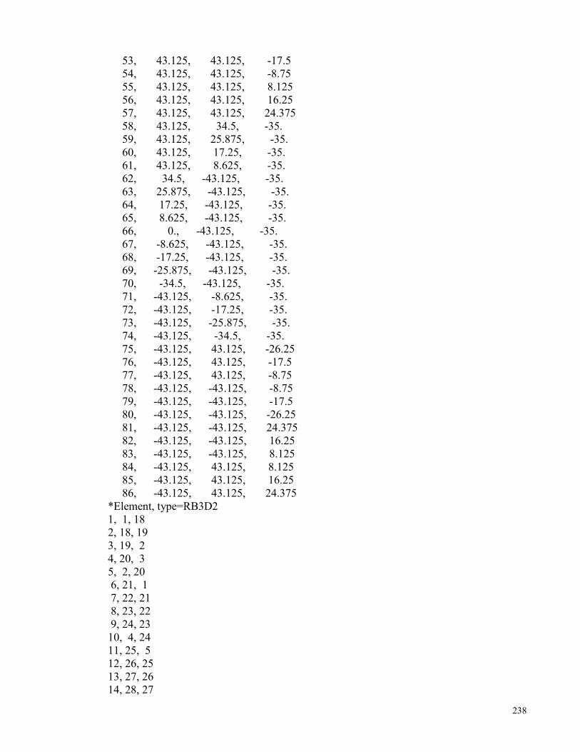
238
53, 43.125, 43.125, -17.5 54, 43.125, 43.125, -8.75 55, 43.125, 43.125, 8.125 56, 43.125, 43.125, 16.25 57, 43.125, 43.125, 24.375 58, 43.125, 34.5, -35. 59, 43.125, 25.875, -35. 60, 43.125, 17.25, -35. 61, 43.125, 8.625, -35. 62, 34.5, -43.125, -35. 63, 25.875, -43.125, -35. 64, 17.25, -43.125, -35. 65, 8.625, -43.125, -35. 66, 0., -43.125, -35. 67, -8.625, -43.125, -35. 68, -17.25, -43.125, -35. 69, -25.875, -43.125, -35. 70, -34.5, -43.125, -35. 71, -43.125, -8.625, -35. 72, -43.125, -17.25, -35. 73, -43.125, -25.875, -35. 74, -43.125, -34.5, -35. 75, -43.125, 43.125, -26.25 76, -43.125, 43.125, -17.5 77, -43.125, 43.125, -8.75 78, -43.125, -43.125, -8.75 79, -43.125, -43.125, -17.5 80, -43.125, -43.125, -26.25 81, -43.125, -43.125, 24.375 82, -43.125, -43.125, 16.25 83, -43.125, -43.125, 8.125 84, -43.125, 43.125, 8.125 85, -43.125, 43.125, 16.25 86, -43.125, 43.125, 24.375 *Element, type=RB3D2 1, 1, 18 2, 18, 19 3, 19, 2 4, 20, 3 5, 2, 20 6, 21, 1 7, 22, 21 8, 23, 22 9, 24, 23 10, 4, 24 11, 25, 5 12, 26, 25 13, 27, 26 14, 28, 27

239
15, 1, 28 16, 6, 29 17, 29, 30 18, 30, 31 19, 31, 32 20, 32, 5 21, 6, 33 22, 33, 34 23, 34, 35 24, 35, 7 25, 36, 8 26, 37, 36 27, 38, 37 28, 7, 38 29, 39, 9 30, 40, 39 31, 41, 40 32, 42, 41 33, 4, 42 34, 9, 43 35, 43, 44 36, 44, 45 37, 45, 46 38, 46, 47 39, 47, 48 40, 48, 49 41, 49, 50 42, 50, 51 43, 51, 10 44, 10, 52 45, 52, 53 46, 53, 54 47, 54, 11 48, 11, 55 49, 55, 56 50, 56, 57 51, 57, 12 52, 58, 10 53, 59, 58 54, 60, 59 55, 61, 60 56, 5, 61 57, 62, 6 58, 63, 62 59, 64, 63 60, 65, 64 61, 66, 65 62, 67, 66 63, 68, 67

240
64, 69, 68 65, 70, 69 66, 13, 70 67, 71, 4 68, 72, 71 69, 73, 72 70, 74, 73 71, 13, 74 72, 9, 75 73, 75, 76 74, 76, 77 75, 77, 14 76, 78, 15 77, 79, 78 78, 80, 79 79, 13, 80 80, 81, 16 81, 82, 81 82, 83, 82 83, 15, 83 84, 14, 84 85, 84, 85 86, 85, 86 87, 86, 17 *Node 87, 0., 0., 3. *Nset, nset=hull-1-RefPt_, internal 87, *Nset, nset=_PickedSet32, internal 87, *Nset, nset=_PickedSet166, generate 1, 86, 1 *Elset, elset=_PickedSet166, generate 1, 87, 1 *Element, type=MASS, elset=_PickedSet32_Inertia-1_MASS_ 88, 87 *Mass, elset=_PickedSet32_Inertia-1_MASS_ **4.05e+07, 8.52E+07, *Element, type=ROTARYI, elset=_PickedSet32_Inertia-1_ROTI_ 89, 87 *RotaryI, elset=_PickedSet32_Inertia-1_ROTI_ **8.221e+10, 8.221e+10, 9.788e+10, 0., 0., 0. 1.67E+11, 1.67E+11, 2.22E+11, 0., 0., 0. *End Instance ** *Nset, nset=_PickedSet165, internal, instance=hull-1 87, *Nset, nset=_PickedSet166, internal, instance=hull-1, generate
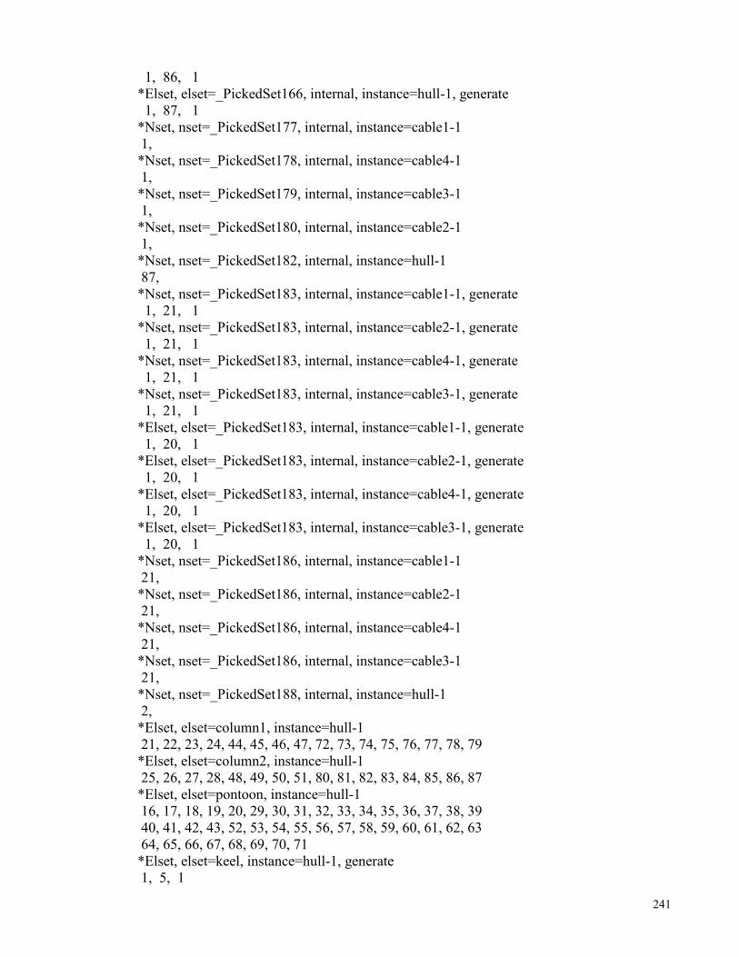
241
1, 86, 1 *Elset, elset=_PickedSet166, internal, instance=hull-1, generate 1, 87, 1 *Nset, nset=_PickedSet177, internal, instance=cable1-1 1, *Nset, nset=_PickedSet178, internal, instance=cable4-1 1, *Nset, nset=_PickedSet179, internal, instance=cable3-1 1, *Nset, nset=_PickedSet180, internal, instance=cable2-1 1, *Nset, nset=_PickedSet182, internal, instance=hull-1 87, *Nset, nset=_PickedSet183, internal, instance=cable1-1, generate 1, 21, 1 *Nset, nset=_PickedSet183, internal, instance=cable2-1, generate 1, 21, 1 *Nset, nset=_PickedSet183, internal, instance=cable4-1, generate 1, 21, 1 *Nset, nset=_PickedSet183, internal, instance=cable3-1, generate 1, 21, 1 *Elset, elset=_PickedSet183, internal, instance=cable1-1, generate 1, 20, 1 *Elset, elset=_PickedSet183, internal, instance=cable2-1, generate 1, 20, 1 *Elset, elset=_PickedSet183, internal, instance=cable4-1, generate 1, 20, 1 *Elset, elset=_PickedSet183, internal, instance=cable3-1, generate 1, 20, 1 *Nset, nset=_PickedSet186, internal, instance=cable1-1 21, *Nset, nset=_PickedSet186, internal, instance=cable2-1 21, *Nset, nset=_PickedSet186, internal, instance=cable4-1 21, *Nset, nset=_PickedSet186, internal, instance=cable3-1 21, *Nset, nset=_PickedSet188, internal, instance=hull-1 2, *Elset, elset=column1, instance=hull-1 21, 22, 23, 24, 44, 45, 46, 47, 72, 73, 74, 75, 76, 77, 78, 79 *Elset, elset=column2, instance=hull-1 25, 26, 27, 28, 48, 49, 50, 51, 80, 81, 82, 83, 84, 85, 86, 87 *Elset, elset=pontoon, instance=hull-1 16, 17, 18, 19, 20, 29, 30, 31, 32, 33, 34, 35, 36, 37, 38, 39 40, 41, 42, 43, 52, 53, 54, 55, 56, 57, 58, 59, 60, 61, 62, 63 64, 65, 66, 67, 68, 69, 70, 71 *Elset, elset=keel, instance=hull-1, generate 1, 5, 1

242
*Elset, elset=braces, instance=hull-1, generate 6, 15, 1 *Elset, elset=cable3, instance=cable1-1, generate 1, 20, 1 *Elset, elset=cable1, instance=cable1-1, generate 1, 20, 1 *Elset, elset=cable2, instance=cable2-1, generate 1, 20, 1 *Elset, elset=cable4, instance=cable4-1, generate 1, 20, 1 *Nset, nset=hullweight,instance=hull-1 87, ** Constraint: Constraint-1 *Rigid Body, ref node=_PickedSet165, elset=_PickedSet166, position=CENTER OF MASS *Element, type=CONN3D2, elset=_Conn-1_CnSet_ 1, hull-1.13, cable1-1.21 *Connector Section, elset=_Conn-1_CnSet_ **Join, beam *Element, type=CONN3D2, elset=_Conn-2_CnSet_ 2, hull-1.6, cable2-1.21 *Connector Section, elset=_Conn-2_CnSet_ **Join, beam *Element, type=CONN3D2, elset=_Conn-3_CnSet_ 3, hull-1.10, cable3-1.21 *Connector Section, elset=_Conn-3_CnSet_ **Join, beam *Element, type=CONN3D2, elset=_Conn-4_CnSet_ 4, hull-1.9, cable4-1.21 *Connector Section, elset=_Conn-4_CnSet_ **Join, beam *End Assembly ** ** CONNECTORS ** ** MATERIALS ** *Material, name=steel *Damping, alpha=0.002259, beta=0.01392 *Density 7800., *Elastic 2.1e+11, 0.28 ** *amplitude, name=dammy
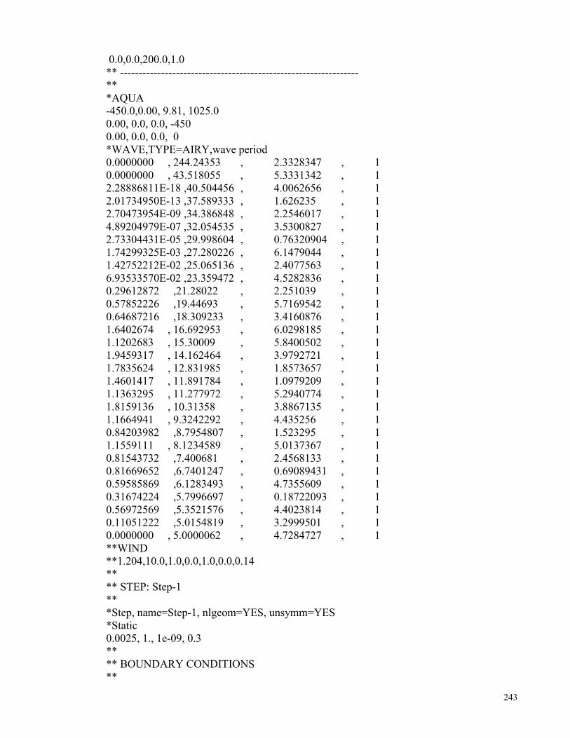
243
0.0,0.0,200.0,1.0 ** ---------------------------------------------------------------- ** *AQUA -450.0,0.00, 9.81, 1025.0 0.00, 0.0, 0.0, -450 0.00, 0.0, 0.0, 0 *WAVE,TYPE=AIRY,wave period 0.0000000 , 244.24353 , 2.3328347 , 1 0.0000000 , 43.518055 , 5.3331342 , 1 2.28886811E-18 ,40.504456 , 4.0062656 , 1 2.01734950E-13 ,37.589333 , 1.626235 , 1 2.70473954E-09 ,34.386848 , 2.2546017 , 1 4.89204979E-07 ,32.054535 , 3.5300827 , 1 2.73304431E-05 ,29.998604 , 0.76320904 , 1 1.74299325E-03 ,27.280226 , 6.1479044 , 1 1.42752212E-02 ,25.065136 , 2.4077563 , 1 6.93533570E-02 ,23.359472 , 4.5282836 , 1 0.29612872 ,21.28022 , 2.251039 , 1 0.57852226 ,19.44693 , 5.7169542 , 1 0.64687216 ,18.309233 , 3.4160876 , 1 1.6402674 , 16.692953 , 6.0298185 , 1 1.1202683 , 15.30009 , 5.8400502 , 1 1.9459317 , 14.162464 , 3.9792721 , 1 1.7835624 , 12.831985 , 1.8573657 , 1 1.4601417 , 11.891784 , 1.0979209 , 1 1.1363295 , 11.277972 , 5.2940774 , 1 1.8159136 , 10.31358 , 3.8867135 , 1 1.1664941 , 9.3242292 , 4.435256 , 1 0.84203982 ,8.7954807 , 1.523295 , 1 1.1559111 , 8.1234589 , 5.0137367 , 1 0.81543732 ,7.400681 , 2.4568133 , 1 0.81669652 ,6.7401247 , 0.69089431 , 1 0.59585869 ,6.1283493 , 4.7355609 , 1 0.31674224 ,5.7996697 , 0.18722093 , 1 0.56972569 ,5.3521576 , 4.4023814 , 1 0.11051222 ,5.0154819 , 3.2999501 , 1 0.0000000 , 5.0000062 , 4.7284727 , 1 **WIND **1.204,10.0,1.0,0.0,1.0,0.0,0.14 ** ** STEP: Step-1 ** *Step, name=Step-1, nlgeom=YES, unsymm=YES *Static 0.0025, 1., 1e-09, 0.3 ** ** BOUNDARY CONDITIONS **

244
** Name: BC-1 Type: Displacement/Rotation *Boundary _PickedSet177, 1, 1 _PickedSet177, 2, 2 _PickedSet177, 3, 3 _PickedSet177, 4, 4 _PickedSet177, 5, 5 _PickedSet177, 6, 6 ** Name: BC-2 Type: Displacement/Rotation *Boundary _PickedSet178, 1, 1 _PickedSet178, 2, 2 _PickedSet178, 3, 3 _PickedSet178, 4, 4 _PickedSet178, 5, 5 _PickedSet178, 6, 6 ** Name: BC-3 Type: Displacement/Rotation *Boundary _PickedSet179, 1, 1 _PickedSet179, 2, 2 _PickedSet179, 3, 3 _PickedSet179, 4, 4 _PickedSet179, 5, 5 _PickedSet179, 6, 6 ** Name: BC-4 Type: Displacement/Rotation *Boundary _PickedSet180, 1, 1 _PickedSet180, 2, 2 _PickedSet180, 3, 3 _PickedSet180, 4, 4 _PickedSet180, 5, 5 _PickedSet180, 6, 6 ** Name: BC-6 Type: Displacement/Rotation *Boundary _PickedSet182, 1, 1 _PickedSet182, 2, 2 _PickedSet182, 3, 3 _PickedSet182, 4, 4 _PickedSet182, 5, 5 _PickedSet182, 6, 6 ** ** LOADS ** ** Name: Load-1 Type: Gravity *Dload _PickedSet183, GRAV, 9.81, 0., 0., -1. ** Name: Load-5 Type: Concentrated force *Cload _PickedSet186, 3, -3.4325e+07
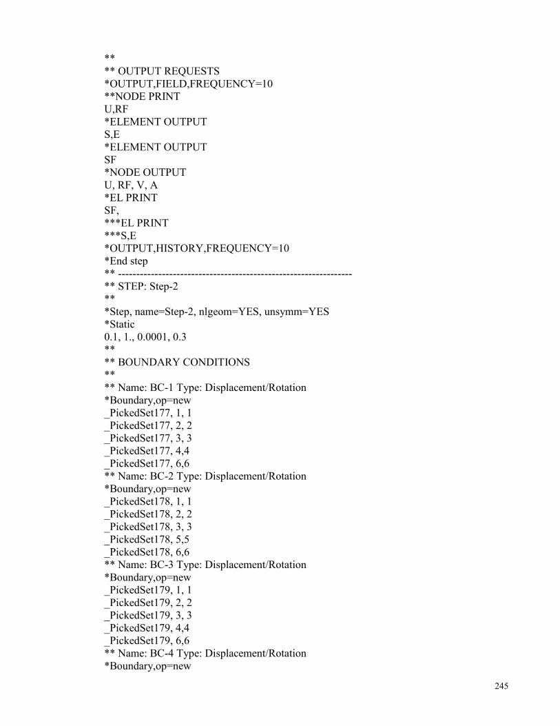
245
** ** OUTPUT REQUESTS *OUTPUT,FIELD,FREQUENCY=10 **NODE PRINT U,RF *ELEMENT OUTPUT S,E *ELEMENT OUTPUT SF *NODE OUTPUT U, RF, V, A *EL PRINT SF, ***EL PRINT ***S,E *OUTPUT,HISTORY,FREQUENCY=10 *End step ** ---------------------------------------------------------------- ** STEP: Step-2 ** *Step, name=Step-2, nlgeom=YES, unsymm=YES *Static 0.1, 1., 0.0001, 0.3 ** ** BOUNDARY CONDITIONS ** ** Name: BC-1 Type: Displacement/Rotation *Boundary,op=new _PickedSet177, 1, 1 _PickedSet177, 2, 2 _PickedSet177, 3, 3 _PickedSet177, 4,4 _PickedSet177, 6,6 ** Name: BC-2 Type: Displacement/Rotation *Boundary,op=new _PickedSet178, 1, 1 _PickedSet178, 2, 2 _PickedSet178, 3, 3 _PickedSet178, 5,5 _PickedSet178, 6,6 ** Name: BC-3 Type: Displacement/Rotation *Boundary,op=new _PickedSet179, 1, 1 _PickedSet179, 2, 2 _PickedSet179, 3, 3 _PickedSet179, 4,4 _PickedSet179, 6,6 ** Name: BC-4 Type: Displacement/Rotation *Boundary,op=new
246
_PickedSet180, 1, 1 _PickedSet180, 2, 2 _PickedSet180, 3, 3 _PickedSet180, 5,5 _PickedSet180, 6,6 ** ** OUTPUT REQUESTS *OUTPUT,FIELD,FREQUENCY=10 **NODE PRINT U,RF *ELEMENT OUTPUT S,E *ELEMENT OUTPUT SF *NODE OUTPUT U, RF, V, A *EL PRINT SF, ***EL PRINT ***S,E *OUTPUT,HISTORY,FREQUENCY=10 *End step ** ---------------------------------------------------------------- ** STEP: Step-3 ** *Step, name=Step-3, nlgeom=YES, unsymm=YES *Static 0.1, 1., 0.0001, 0.3 ** ** BOUNDARY CONDITIONS ** ** Name: BC-1 Type: Displacement/Rotation *Boundary,op=new _PickedSet177, 1, 1 _PickedSet177, 2, 2 _PickedSet177, 3, 3, -0.140969 _PickedSet177, 4,4 _PickedSet177, 6,6 ** Name: BC-2 Type: Displacement/Rotation *Boundary,op=new _PickedSet178, 1, 1 _PickedSet178, 2, 2 _PickedSet178, 3, 3, -0.140969 _PickedSet178, 5,5 _PickedSet178, 6,6 ** Name: BC-3 Type: Displacement/Rotation *Boundary,op=new _PickedSet179, 1, 1 _PickedSet179, 2, 2

247
_PickedSet179, 3, 3, -0.140969 _PickedSet179, 4,4 _PickedSet179, 6,6 ** Name: BC-4 Type: Displacement/Rotation *Boundary,op=new _PickedSet180, 1, 1 _PickedSet180, 2, 2 _PickedSet180, 3, 3,-0.140969 _PickedSet180, 5,5 _PickedSet180, 6,6 ** ** LOADS ** Name: Load-6 Type: Concentrated force *Dload,op=new ***Selfweight on Tendons _PickedSet183, GRAV, 9.81, 0., 0., -1. **Point Buoyancy load *Dload, OP=NEW _PickedSet183,PB , 1.0,0.71 *Cload,op=new _PickedSet188, 3, 5.346e+08 ***************** **Mass per unit length on tendons in N/m *Dload, OP=NEW _PickedSet183, PZ, -30124.5 ** *Cload,op=new hullweight, 3, -3.973e+08 ** OUTPUT REQUESTS *OUTPUT,FIELD,FREQUENCY=10 **NODE PRINT U,RF *ELEMENT OUTPUT S,E *ELEMENT OUTPUT SF *NODE OUTPUT U, RF, V, A *EL PRINT SF, ***EL PRINT ***S,E *OUTPUT,HISTORY,FREQUENCY=10 *End step ************************************* ** STEP: Step-4 ** *Step, name=Step-4, nlgeom=YES, inc=100000, unsymm=YES *Dynamic,alpha=-0.05,haftol=1e7

248
0.01, 6000.0, 1e-4,3.0 ** ** LOADS *amplitude, name=VelocityX-Amplitude, Time=Total Time 0.0,0.0,200.0,30.00 *amplitude, name=VelocityY-Amplitude, Time=Total Time 0.0,0.0,200.0,0.0 ** *Dload,amplitude=dammy column1, FDD,1.0,16.88,1.0 column1, FI,1.0,16.88,2.0,1.0 pontoon, FDD,1.0,7.50,1.0 pontoon, FI,1.0,7.50,2.0,1.0 cable1, FDD,1.0,0.71,1.0 cable1, FI,1.0,0.71,2.0,1.0 cable2, FDD,1.0,0.71,1.0 cable2, FI,1.0,0.71,2.0,1.0 cable3, FDD,1.0,0.71,1.0 cable3, FI,1.0,0.71,2.0,1.0 cable4, FDD,1.0,0.71,1.0 cable4, FI,1.0,0.71,2.0,1.0 **column2, WDD,1.0, 16.88, 2.0, 1.0, VelocityX-Amplitude, VelocityY-Amplitude *restart,write,overlay *OUTPUT,FIELD,FREQUENCY=10 **NODE PRINT U,RF *ELEMENT OUTPUT S,E *ELEMENT OUTPUT SF *NODE OUTPUT U, RF, V, A *EL PRINT SF, ***EL PRINT ***S,E *OUTPUT,HISTORY,FREQUENCY=10 *End step

249
Appendix C
C PROGRAM TO GENERATE SPECTRUM USING TIME HISTORY PROGRAM SDFH COMPLEXA(4096),SG,XG DIMENSION SP(10000),B(10000),X(10000) OPEN(UNIT=5,FILE='surge.dat') OPEN(UNIT=6,FILE='psdf.dat') c OPEN(UNIT=7,FILE='A.R7') NP = 12 TI = 0.2 IJ = 2 DT = TI NB = 2**NP DO 1 I = 1,NB READ(5,*) X(I) 1 CONTINUE DO 2 K = 1,NB C WRITE(5,*) B(I),X(I) 2 CONTINUE NT = NB NBS = NB/2+1 TT = DT*NT BW = 1.0/TT TPI = 4.0*ATAN(1.0) XX = 0.0 DO 500 I = 1,NT XX = X(I)+XX 500 CONTINUE SNT = FLOAT(NT) XAV = XX/SNT DO 501 I = 1,NT X(I) = X(I)-XAV 501 CONTINUE DO 502 I = 1,NB 502 A(I) =CMPLX(0.0,0.0) DO 503 I = 1,NT XX = X(I) A(I) = CMPLX(XX,0.0) 503 CONTINUE CALL FFT(NB,NP,A) DO 516 I = 1,NB A(I) = A(I)*CONJG(A(I)) 516 CONTINUE DO 535 I = 1,NBS XG = NB*DT*A(I)/(2.0*TPI) A(I) = XG*NB/SNT 535 CONTINUE M = BW*TT/2.0-1/2.
250
M = M+1 C WRITE(6,*)M DTT = 2.0*TPI/TT C WRITE(6,*)DTT,NBS DO 555 I = 1,NBS SX = A(I) DO 556 J = 1,M II = J+I IF(II.GT.NBS) GO TO 560 SX = SX+A(I+J) 560 JJ = I-J IF(JJ.LE.0) GO TO 562 SX = SX+A(I-J) GO TO 573 562 KK = 2-JJ SX = SX+CONJG(A(KK)) 573 DUMMY = 0.0 556 CONTINUE SP(I) = 2.0*REAL(SX) SP(I) = SP(I)/FLOAT(2*M+1) TD = 2.0*TPI/TT*I WRITE(6,10)TD,SP(I) 10 FORMAT(F12.5,3X,E18.6) 555 CONTINUE STOP END C ******************************************* SUBROUTINE FFT(N,M,A) COMPLEX A(4096),U,W,H DO 1 I = 1,N 1 A(I) = A(I)/N NV2 = N/2 NM1 = N-1 J = 1 DO 30 I = 1,NM1 IF(I.GT.J) GO TO 10 H = A(J) A(J) = A(I) A(I) = H 10 K = NV2 20 IF(K.GE.J) GO TO 30 J = J-K K = K/2 GO TO 20 30 J = J+K PI = 4.0*ATAN(1.0) DO 50 L = 1,M LE = 2**L LE1 = LE/2

251
U = CMPLX(1.0,0.0) W = CMPLX(COS(PI/LE1),-SIN(PI/LE1)) DO 50 J = 1,LE1 DO 40 I = J,N,LE IP = I+LE1 H = A(IP)*U A(IP) = A(I)-H A(I) = A(I)+H 40 CONTINUE U = U*W 50 CONTINUE RETURN END


