49
Stochastic Hybrid Systems: Models and Applications Hendra I. Nurdin

Stochastic Hybrid Systems: Models andApplications
Hendra I. Nurdin

ii
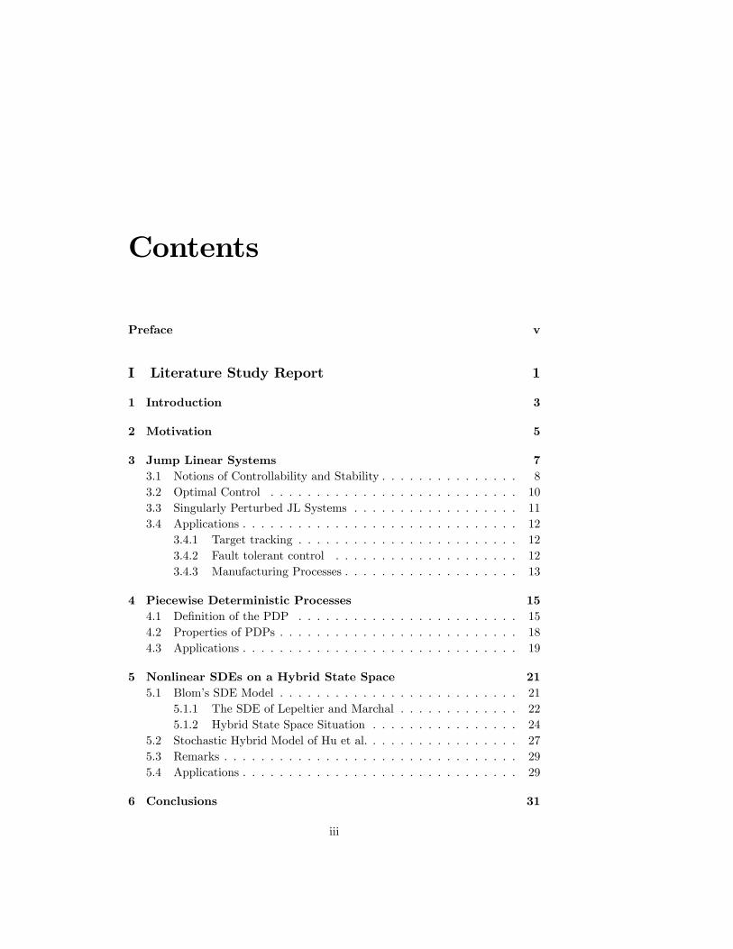
Contents
Preface v
I Literature Study Report 1
1 Introduction 3
2 Motivation 5
3 Jump Linear Systems 73.1 Notions of Controllability and Stability . . . . . . . . . . . . . . . 83.2 Optimal Control . . . . . . . . . . . . . . . . . . . . . . . . . . . 103.3 Singularly Perturbed JL Systems . . . . . . . . . . . . . . . . . . 113.4 Applications . . . . . . . . . . . . . . . . . . . . . . . . . . . . . . 12
3.4.1 Target tracking . . . . . . . . . . . . . . . . . . . . . . . . 123.4.2 Fault tolerant control . . . . . . . . . . . . . . . . . . . . 123.4.3 Manufacturing Processes . . . . . . . . . . . . . . . . . . . 13
4 Piecewise Deterministic Processes 154.1 De�nition of the PDP . . . . . . . . . . . . . . . . . . . . . . . . 154.2 Properties of PDPs . . . . . . . . . . . . . . . . . . . . . . . . . . 184.3 Applications . . . . . . . . . . . . . . . . . . . . . . . . . . . . . . 19
5 Nonlinear SDEs on a Hybrid State Space 215.1 Blom�s SDE Model . . . . . . . . . . . . . . . . . . . . . . . . . . 21
5.1.1 The SDE of Lepeltier and Marchal . . . . . . . . . . . . . 225.1.2 Hybrid State Space Situation . . . . . . . . . . . . . . . . 24
5.2 Stochastic Hybrid Model of Hu et al. . . . . . . . . . . . . . . . . 275.3 Remarks . . . . . . . . . . . . . . . . . . . . . . . . . . . . . . . . 295.4 Applications . . . . . . . . . . . . . . . . . . . . . . . . . . . . . . 29
6 Conclusions 31
iii
iv CONTENTS
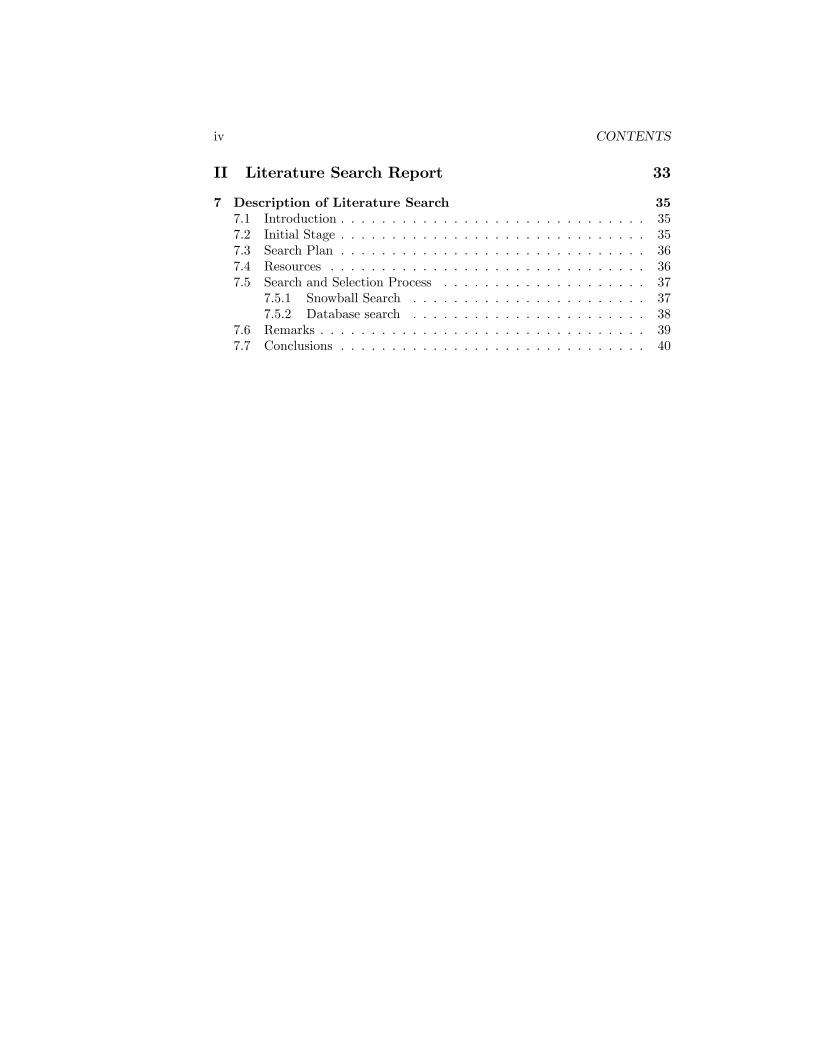
II Literature Search Report 33
7 Description of Literature Search 357.1 Introduction . . . . . . . . . . . . . . . . . . . . . . . . . . . . . . 357.2 Initial Stage . . . . . . . . . . . . . . . . . . . . . . . . . . . . . . 357.3 Search Plan . . . . . . . . . . . . . . . . . . . . . . . . . . . . . . 367.4 Resources . . . . . . . . . . . . . . . . . . . . . . . . . . . . . . . 367.5 Search and Selection Process . . . . . . . . . . . . . . . . . . . . 37
7.5.1 Snowball Search . . . . . . . . . . . . . . . . . . . . . . . 377.5.2 Database search . . . . . . . . . . . . . . . . . . . . . . . 38
7.6 Remarks . . . . . . . . . . . . . . . . . . . . . . . . . . . . . . . . 397.7 Conclusions . . . . . . . . . . . . . . . . . . . . . . . . . . . . . . 40

Preface
This report is a summary of the literature search and study that the authorcarried out on stochastic hybrid systems and its applications in the fourth termof the M.Sc programme in Engineering Mathematics at the Faculty of Mathe-matical Sciences, University of Twente.The report is divided into two parts. The �rst part, consisting of chapters
1 through 6, contains the result of the literature study, i.e. the informationthat was absorbed by the author from a selected number of literatures. Thesecond part, consisting of only chapter 7, explains the search process and relatedliteratures that were found.The author would like to express his gratitude to a number of people who
have made contributions to this study. First of all the author would like tothank his supervisor Prof. Dr. Arunabha Bagchi for his support, for providinginitial references and for the interesting discussions on the stochastic hybridsystems that appear in this report. Secondly the author is also indebted to thefaculty librarian drs. R.J. van Wissen who was very helpful in providing theauthor with knowledge about search facilities and available databases and whoalso assisted the author in obtaining a number of literatures. Finally the authorwould like to thank Ph.D student Anak Agung Julius for providing two relatedmaterials and Prof. Dr. Arjan van der Schaft for providing a copy of a paperby M.H.A. Davis.
Enschede, November 2001
Hendra I. Nurdin
v

vi PREFACE

Part I
Literature Study Report
1


Chapter 1
Introduction
Broadly speaking, hybrid systems are dynamical systems containing both dis-crete and Euclidean valued variables. Discrete variables are variables that canonly take on speci�c values on a certain countable set such as N = f1; 2; 3; :::g orA = f0:12; 4:1; 6:5; 8:6g. On the other hand, the Euclidean variables can takeon any value in a set T � R and not restricted to some discrete set of points.The discrete and Euclidean dynamics not only co-exist in the same system butthey may also interact, thus the Euclidean variables may in�uence the dynamicsof the discrete variables and vice versa. Hybrid systems arise naturally in manydi¤erent research communities such as in the computer science, modeling andsimulation, and systems and control community[Scha00].Many di¤erent researchers over the years have been working separately on
hybrid systems and it was only recently that e¤ort started towards developinga uni�ed approach to hybrid systems[Scha00]. Based on the nature of the vari-ables involved, hybrid systems can further be grouped into deterministic hybridsystems (DHSs) and stochastic hybrid systems (SHSs). In DHS, which is theprimary concern in [Scha00], all the variables involved are assumed to be de-terministic, while in SHS the variables are random. Although the deterministicframework does capture many characteristics of actual systems in practice, themissing factor of randomness will be a fatal �aw because these systems work inan inherently uncertain real-world environment. This report is primarily a sur-vey of continuous time stochastic hybrid systems, in particular it is concernedwith the type of stochastic hybrid systems that have been introduced over theyears and the status of current research in the �eld.The concept of SHS is not something new, although these systems were
coined as �stochastic hybrid systems�only recently. Pioneering work in the early60s and 70s on models incorporating mixed Euclidean and discrete variables andrandomness can be traced to researchers like Krasovskii and Lidskii, Sworderand Wonham[Mari90]. Extensions of their work can be found in papers such as[Ji90] and [Ji92]. The early SHS models and those that were introduced lateron, such as piecewise deterministic process models and stochastic di¤erentialequation models, will be reviewed to some extent in this report.
3

4 CHAPTER 1. INTRODUCTION
The �rst part of the report is organized as follows. In Chapter 2, motivationin carrying out the literature study is given. Chapter 3 deals with the �rstmodels to appear, i.e. the jump linear models, and its applications. Piecewisedeteministic processes is the central theme of Chapter 4 while SDE models arediscussed in Chapter 5. Finally conclusions from the literature study are givenin Chapter 6.

Chapter 2
Motivation
Over the years stochastic hybrid systems models have been successfully appliedto represent abrupt value changes in the parameters of economic systems, com-ponent/sensor failures in power systems, aircraft and manufacturing systems,sudden system connection reorganization in power systems and large �exiblestructures, pilot commands in target tracking, and sudden environmental dis-turbances like clouds in isolation levels of a solar receiver[Tsai97]. Since SHSmodels can adequately describe situations where the system�s characteristics(i.e., parameters of the associated dynamical equations) change due to fail-ure of a component, several researchers view that such models are importantto achieve truly fault tolerant behavior in control systems[Tsai97]. More re-cently, Blom et al. have proposed the development of a SHS to model gen-eral air tra¢ c encounter situations in advanced Air Tra¢ c Management (ATM)operations[Blom99][Blom01]. The SHS model then serves as basis to performaccident risk assessment of an advanced ATM operation. In [Blom01] SHSsbased on two classes of non-linear continuous time stochastic hybrid dynamicalmodels, the piecewise deterministic Markov processes (PDPs) and stochasticdi¤erential equations (SDEs) on a hybrid state space, are discussed.This report is essentially a survey of some of the work that have been done
in the �eld of stochastic hybrid systems. PDPs and hybrid SDEs mentionedpreviously along with other relevant SHS models that have appeared in theliterature and its applications are reviewed in the following chapters.
5

6 CHAPTER 2. MOTIVATION

Chapter 3
Jump Linear Systems
The earliest SHS models in the literature are based on piecewise linear timeinvariant (LTI) state space systems. Hence it is not surprising that there is quitea large volume of literature available on the subject. This chapter summarizessome of the main results of the research.Let rt denote the discrete valued component of the hybrid state, called the
regime or form, that take on values in S = f1; 2; :::; Ng while xt denotes theEuclidean component that take on values in Rn. It follows that the state spaceof the system is S�Rn. The dynamics of the Euclidean component is piecewiselinear and is given by:
�xt = A(rt)xt +B(rt)ut
yt = C(rt)xt(3.1)
where ut; yt are, respectively, the control input to the system and the outputof the system, while are A, B, C are matrices of corresponding dimensions.The dynamics explicitly depend on the value taken by the regime, thus whenthe regime changes the dynamics of the system will also change. The situationthat is of interest is one where the changes (or jumps) in the regime occur ina random fashion. To describe the jump dynamics let �t 2 RN (N=card(S))with components �ti = 1 when rt = 1 and �ti = 0 otherwise, i = 1; 2; :::; N .The indicator is piecewise constant and the model usually taken for regimetransitions is a Markov chain given by:
d�t = �0�tdt+ dMt
whereMt is an �-martingale on a probability space (;�; P ) with an associatednon-decreasing �-algebras �t 2 �, and � the chain generator, an N�N matrix.The entries �ij , i; j = 1; ::; N of � are interpreted as the transition rates
P (rt+� = jjrt = i) =
�1 + �ij�+ o(�) i = j
�ij�+ o(�) i 6= j
7

8 CHAPTER 3. JUMP LINEAR SYSTEMS
The above jump linear (JL) model is a model where noise that can appear inthe dynamics and output measurement are not accounted for. A more generalmodel is the following:
dxt = A(rt)xtdt+B(rt)utdt+D(xt; rt)dw1t + E(ut; rt)dw1t + F (rt)dw3tdyt = C(rt)xtdt+H(rt)dvt
(3.2)
where wit, i = 1; 2; 3 are independent Wiener processes (Brownian motion) onRni and D, E, and F are matrices of corresponding dimensions. The stochasticdi¤erential equation in (3.2) should be interpreted in the Ito sense. D and Eare usually restricted to have the following form:
D(xt; rt) =nPk=1
xktDk(rt)
E(xt; rt) =nPk=1
uktEk(rt)
where xkt and ukt are the k-th component of x and u at time k, respectively.Hence the dynamics switches from one Ito stochastic di¤erential equation toanother. It should be mentioned that at the jump times, the times when theregime switches, xt is usually considered continuous although sometimes it ismodeled that xt experiences a discontinuity of random magnitude when theregime changes ([Mari87] or Section 5.4 in [Mari90]). Note that the pair (rt; xt)by de�nition constitutes a Markov pair.The monograph [Mari90] provides a summary of work that has been done
on jump linear systems up to around 1989. Most of the material discussed inthis chapter are taken from there. The research that have been done on thesesystems can broadly be divided into three themes:
1. Development of suitable notions of controllability, stabilizability and othernotions from LTI systems to JL systems.
2. Deriving optimal controllers for JL systems
3. Analysis of singularly perturbed JL systems
3.1 Notions of Controllability and Stability
In deterministic linear time invariant systems, the notion of controllability in-troduced by Kalman plays an important role. Extending such a concept tostochastic systems like JL systems is di¢ cult to establish since a similar notionor several notions can be de�ned depending on the way randomness is takeninto account. In this section some notions of controllability and stability thathave been introduced for JL systems are discussed. Although these concepts
3.1. NOTIONS OF CONTROLLABILITY AND STABILITY 9
were developed for jump linear systems, it is possible that they can be extendedto other types of stochastic systems.Mariton introduced the notion of "-controllability in which an initial state x0
is said to be "-controllable with probability � over the time interval [t0; tf ] if thereexists a control law u(t; x) such that P (jjxtf jj2 � "jx(t0) = x0) � 1 � �. Usingthis de�nition su¢ cient conditions for the "-controllability of a hybrid system ofthe type (3.1) were derived. A property of "-controllability is that deterministiccontrollability of all the regimes implies "-controllability, but the converse isnot true. The notion of "-controllability is a kind of relative controllability, itdoes not give the dichotomic yes or no controllability classi�cation as in thedeterministic setting, rather it measures a relative and continuous degree ofcontrollability.A global notion of controllability for JL system has also been proposed
whereby a JL system (3.1) can be categorized as being weakly controllable,controllable, or strongly controllable. Let xt(x0; u) be the state trajectory start-ing at x(t0) = x0 under the control u. A system is called weakly control-lable if for 8x0 2 Rn, 8x1 2 Rn and 8" > 0 there exists an almost surely�nite random time T and an admissible control law over [t0; T ] such thatP (jjxT (xo; u) � x1jj � ") > 0. The system is called controllable if the previ-ous probability can be made equal to 1 and strongly controllable if it is weaklycontrollable and the hitting time TH = inffT > 0; jjxT (xo; u) � x1jj � "g has�nite expectation. Necessary and su¢ cient condition for strong controllabilitycan be obtained through a rank test, in a similar spirit to the deterministiccase. For weak controllability the deterministic controllability of each regime isa su¢ cient condition, but the system can be controllable in the weak sense evenif all the regimes are uncontrollable in the deterministic sense.
In [Mari 88], Mariton introduces two other concepts of stochastic stabil-ity for JL systems: almost sure sample path stability and moments stability.Therein su¢ cient and necessary condition for p-th moment stability and a suf-�cient condition for almost sure stability were derived based on the ideas ofLyapunov exponents and Coppel�s dichotomy. For this type of stochastic sta-bility it is quite interesting to note that deteministic stability of the regimes isneither a necessary nor su¢ cient condition. Ji and Chizeck[Ji90] introduced thenotion of stochastic stabilizability and controllability in a mean square sense: asystem (3.1) is stochastically stabilizable if there exists a linear feedback law ofthe form u(t) = �L(r(t))x(t) which drives the state x from any initial (x0; r0)asymptotically to the origin in a mean square sense, while stochastic controlla-bility means the state can driven to the �-neighbourhood of the origin in a �nitetime T > 0 with control u(t) = �L(r(t))x(t). Note that stochastic controllabil-ity implies stochastic stabilizability but the connverse is not true. Except forsome special cases, it is not possible to drive the state x to the origin in �nitetime. Ji and Chizeck also derived necessary and su¢ cient conditions for stabi-lizability and controllability and also proposed extensions of the dual conceptof stochastic observability and detectability along with necessary and su¢ cientconditions. Investigation of the various kinds of stability of a homogeneousJL system (B = 0) termed asymptotic mean square stability, exponential mean

10 CHAPTER 3. JUMP LINEAR SYSTEMS
square stability, stochastic stability and almost sure (asymptotic) stability can befound in [Feng92]. It is shown that the �rst three type of stability are equivalentand that all three imply the last type.A study of the stability property of a subclass of (3.2) of the form
dxt = A(rt)xtdt+ �(xt; rt)dwt
is elaborated in [Basa96]. For this purpose the notion of stability in distributionwas introduced. A process xt is said to be stable in distribution if there exists aprobability measure �(� � f�g) such that its transition probability p(t; x; i; dy �fjg) converges weakly to �(dy � fjg) as t ! 1 for every (i; x) 2 S � Rn.This notion of stability is more relevant than the mean square types of stabilitythat were discussed in the previous paragraph when considering the additiveperturbation term wt. In the same paper some conditions are derived such thatxt is asymptotically stable if the unperturbed system is stable. Furthermore itis shown that if the unperturbed system is not stable, under some conditionsthe system can be made stable by adding a perturbation.
3.2 Optimal Control
In the literature, many researchers have addressed the problem of optimal con-trol of JL systems. Jump linear quadratic (JLQ) regulators have been derivedfor noiseless JL systems that minimize the cost criterion
EftfZt0
(x0tQ(rt)xt + u0R(rt)u)dtjx0; i0g
for some starting time t0 and end time tf , Q(rt) � 0 and R(rt) > 0, basedon the principle of dynamic programming and the maximum principle that hasbeen adapted to stochastic optimization (see [Mari90], Chapter 3). The resultbears some similarity to linear quadratic regulators for deterministic systems inthe sense that the optimal controller turns out to be a state feedback controllerand there is a Riccati like di¤erential equation (with additional terms due tothe presence of the underlying Markov chain) that must be solved. The statefeedback controller has a dependence on the regime and hence there is a di¤erentcontroller for each regime. The case of in�nite time horizon (t0 !1) has alsobeen considered, conditions have been obtained under which the steady statevalue of the solution to the JL Riccati exists and it has been shown how theclosed loop dynamics are exponentially stable in the mean square sense understochastic stabilizability and detectability conditions[Ji90]. The JLQ regulatoris unrealistic in the sense that in practice information about the states or regimeof a system is not always available, hence there have also been work done in�nding sub-optimal regulators such as the optimal switching output feedback(regime can be perfectly observed but only part of the state can be measured

3.3. SINGULARLY PERTURBED JL SYSTEMS 11
through the output of the system) and optimal non-switching feedback (statefeedback without dependence on the regime).An extension of the �nite horizon JLQ regulator to the more general model
(3.2) is called the jump linear quadratic gaussian (JLQG) regulator, the gaussianterm coming from the fact that it is assumed that the noise processes in thesystem are independent and have gaussian distribution. In the case where thestates and regimes are directly observable, it turns out once again that the op-timal regulator is in the form of a state feedback accompanied by a Riccati likedi¤erential equation. If the regimes are observable but states are not and theonly information available is the noisy system output, a modi�ed Kalman �lterthat takes into account switches in the regime has been derived to estimate thesystem states. The estimated states is then fed into the JLQG controller, replac-ing the real states. Remarkably, under the fact that the regime is observable,the notion of equivalence certainty and the separation theorem well known inthe usual LQ and LQG problems also hold in this case. Hence estimator designand controller design can be separated, and the controller be designed as if theactual states were available for feedback.In the general model it was assumed that the noise processes are in the form
of continuous Wiener processes. In practice there could be present another typeof noise which appears at discrete random instants and is impulsive in nature.Due to its impulsive nature it results in discontinuity of the states of the JLsystem at the jump times. Typically for a spacecraft, this corresponds to im-pingement of meteorites at the solar panels. This type of disturbance can bemodeled as a Poisson process. An optimal regulator for a system with this kindof disturbance can also be derived based on the technique of dynamic program-ming and knowledge of the in�nitesimal generator of the process[Mari87].
3.3 Singularly Perturbed JL Systems
Properties of JL systems with singular perturbation have been studied in theliterature[Tsai92][Tsai97]. In such systems, the dynamics of the Euclidean statesis described by:
�xt = A11(rt)xt +A12(rt)zt +B1(rt)ut
��zt = A21(rt)xt +A22(rt)zt +B2(rt)ut
(3.3)
where � is a small parameter (0 < � << 1). The transition probability matrixof the process rt satisfy the �rst order matrix equation:
dP (t)
dt= P (t)(
1
�F +G); P (t0) = I (3.4)
where it is assumed that (0 < � << 1) and that F , G, and 1�F + G are such
that rt is irreducible. The set S is partitioned into n subsets Si of stronglyinteracting states, i = 1 : : : n. Approximations to the solutions of (3.3) have

12 CHAPTER 3. JUMP LINEAR SYSTEMS
been derived based on probabilistic averaging theory and aggregate models havebeen developed[Tsai92]. Aggregation means that each of the strongly interactingstates in Si are considered as to be one single aggregate state, so that over alonger period the system can be viewed as having n instead of N discrete states.Stochastic stabilizability and controllability of the system (3.1) whose Markovchain transition is governed by (3.4) has been investigated and a near optimumJLQ controller has been derived based on a perturbation method under theassumption that B(rt 2 Si) = Bi [Tsai97]. For a more general case where theprevious assumption is not satis�ed an aggregation method is used to derive anear optimum control law.
3.4 Applications
In this section some situations where the jump linear models arise in practiceare discussed.
3.4.1 Target tracking
JL systems appears in so called evasive tracking problems where it is desiredto keep track of an object manouvering very quickly to evade its pursuer. Inthis situation there are usually sudden changes in acceleration of the the target.The trajectory can typically divided into sections when the aircraft �ies withan almost constant acceleration, bank angle and �ight path angle. The regimesof �ight that are usually considered are ascending �ight after take o¤, turning,accelerated �ight, uniform cruise motion or descending approach �ight. Eachof these regimes of �ight can be associated with some element of a discrete setsuch as S = f1; 2; :::g. Depending on the current �ight regime, the coe¢ cientof the dynamic model have to be adjusted. From the point of view of thetracker/pursuer the regime changes are perceived as being random. Hence thissystem constitutes a JL system if the motion of the aircraft at every regime canbe represented by some set of linear di¤erential equations.
3.4.2 Fault tolerant control
Large complex control systems which consist of a large number of sensors andactuators are very prone to component failure. In order to make the systemreliable despite the failures, redundancy has to be built into the system and aredundancy management system then installed to perform detection and iso-lation of the failures recon�guration of the remaining components and of thecontrol algorithms. To be able to analyze such a kind of system a clear de-scription of the occurence of failure and its e¤ect on the system is necessary.Assuming that the whole system can be considered linear, this can be done byadopting a JL system framework by splitting the operating area of the systeminto distinct regimes. Failures will then appear as random discrete events thatcause a transition, or a jump, of the regime.

3.4. APPLICATIONS 13
3.4.3 Manufacturing Processes
Some manufacturing processes can be suitably modeled by JL systems. Suchprocesses are intrisically hybrid, they evolve on a product space Rn � N � S.The N is well suited to describe the number of products manufactured, while theEuclidean states may represent variables such as machine power consumptionor the storage of raw materials. The discrete state S identi�es the operatingsituation such as the number of machines that are functional or the situation inwhich speci�c machines are operational while others are not.

14 CHAPTER 3. JUMP LINEAR SYSTEMS

Chapter 4
Piecewise DeterministicProcesses
Davis in 1984 [Davi84] introduced a class of stochastic models in which the ran-domness appear as point events, i.e. there is a sequence of random occurencesat �xed or random times T1 < T2 < T3 < ::: but there is no additional com-ponent of uncertainty between these times. Davis termed the class of processeshaving this property as piecewise deterministic Markov processes (PDPs). Thisclass is su¢ ciently general to cover a wide variety of applied problems as specialcases. It is more general than the jump linear models discussed in the previouschapter. Constructing the PDP model corresponding to a particular applicationproceeds by way of one or both of two well known principles: the inclusion ofsupplementary variables to turn an initially non-Markov process into a Markovprocess, and the use of indicator variables to keep track of the various possi-ble �con�gurations�of the system under study. A PDP essentially consists ofa mixture of deterministic motion and random jumps. Davis has written anexcellent research monograph on PDPs, [Davi93], which covers the basic theoryand applications of PDPs.
4.1 De�nition of the PDP
Let K be a countable set and d a function mapping from K into the naturalnumbers N. For each v 2 K, let E0v be an open subset of Rd(v) and de�ne E0as the disjoint union of these subsets:
E0 =Sv2K
E0v = f(v; �) : v 2 K; � 2 E0vg
For each v 2 K, Xv is a given locally Lipschitz continuous vector �eld in E0v ;determining a �ow �v(t; �). On a point of notation, any function h : E
0 ! Ris identi�ed with its component function hv : E0v ! R and Xh(x) is written inplace of Xvhv(�) for x = (v; �) 2 E0: For x = (v; �) de�ne
15

16 CHAPTER 4. PIECEWISE DETERMINISTIC PROCESSES
t�(x) =
�infft > 0 : �v(t; �) 2 @E0vg1 if no such time exists
Here @E0v is the boundary: @E0v = �EvnE0v , where �Ev is the closure of E0v . In
Section 27 of [Davi93], it is veri�ed that t� is a Borel measurable function. If t1denotes the explosion time of the �ow �v(�; �), then it is assumed that t1 =1when t�(x) =1, thus e¤ectively ruling out explosions. Now de�ne
@�E0v = fz 2 @E0v : z = �v(�t; �) for some � 2 E0v , t > 0gand @1E0v = @�E0vn@+E0v : Let Ev = E0v [ @1E0v , E = [vEv and
�� = [v@+E0v
The set E will be the state space for the PDP; it is a countable union ofBorel sets of Euclidean space. Let E denote the �-�eld of subsets A of E takingthe form A = [vAv, where Av is a Borel set of Ev. It can then be shown that(E; E) is Borel space, i.e. a Borel subset of a complete separable metric space.The vector �eld X determines the motion of the PDP between jumps. The
jump mechanism is determined by two further functions, the jump rate � and thetransition measure Q: The triple (X; �;Q) is called the local characteristics ofthe PDP. The jump rate � : E ! R+ is a measurable function such that for eachx = (v; �) 2 E there exists "(x) > 0 such that the function s ! �(v; �v(s; �))is integrable on [0; "(x)[. The transition measure Q maps E [ �� into the setP(E) of probability measures on (E; E) with the properties that:
1. for each �xed A 2 E the map x! Q(A;x) is measurable.
2. Q(fxg; x) = 0:
Let (;A; P ) be the Hilbert cube, i.e. the canonical space for a sequence U1,U2, .... of independent U [0; 1] distributed random variables. The sample pathof a stochastic process fxt(!); t > 0g with values in E, starting from a �xedinitial state x = (v; �) 2 E is de�ned as follows. Let
F (t; x) = I(t<t�(x)) exp(�tR0
�(�; �v(s; �))ds) (4.1)
be the survivor function of the �rst jump time T1 of the process. Now let
1(u; x) =
�infft : F (t; x) � ug
+1 if the above set is empty
and de�ne S1(!) = T1(!) = 1(U1(!); x). Then P (T1 > t) = F (t; x). Let 2 : [0; 1]�(E[��)! E be a measurable function such that l �12 (A) = Q(A;x)for A 2 B(E), where l is the Lebesque measure on [0,1] and B(E) is the Borelset of E. The sample xt(!) up to the �rst jump time is now de�ned as follows:if T1(!) =1 : xt(!) = �(v; �v(t; �)); t � 0

4.1. DEFINITION OF THE PDP 17
if T1(!) <1 :xt(!) = �(v; �v(t; �)); 0 � t < T1(!)xT1(!) = 2(U2(!); (v; �v(T1(!); �)))
The process now restarts from xT1(!) in the same fashion. Therefore de�ne:
S2(!) = 1(U3(!); xT1(!))
T2(!) = T1(!) + S2(!)
Let (v0; � 0) = xT1(!). If T2(!) =1 then obviously
xt(!) = �(v; �v(t; �)); 0 � t < T1(!), t � T1(!)
but if T2(!) =1
xt(!) = �(v0; �v0(t� T1(!); � 0)); T1(!) � t < T2(!)
xT2(!) = 2(U4(!); (v0; �v0(S2(!); �
0)))
and so on. This de�nes a map from into the set of sequences (S1(!); Z1(!); :::; Sk0(!)),where k0 = minfk : Sk(!) = 1g(= 1 if Sk(!) < 1 for all k) and Zk(!) =xTk(!) as de�ned above. Denote Nt(!) =
Pk
I(t�Tk).
Assumption 4.1 For every starting point x 2 E, ENt <1 for all t 2 R+.
Proposition 4.1 Suppose that � is bounded, i.e. �(x) � c <1 for all x 2 E.The previous assumption holds if (1) or (2) below is satis�ed
1. There are no �active�boundaries: t�(x) =1 for all x 2 E.
2. For some " > 0; Q(A";x) = 1 for all x 2 ��, where A" = fx 2 E :t�(x) � "g.
Finally note that it may not be necessary to specify Q(�; x) on all of ��:Consider the case
� = fx = (v; �) 2 �� : Py(T1 = t) > 0 for some t > 0; with y = (v; �v(�t; �))g
It is quite clear that x 2 � i¤ Py(T1 = t)! 1 as t # 0. Points in ��= � are, withprobability 1, not hit by the process from any starting point and it is thereforenot necessary to specify Q on ��= �.Below is a summary of the standard conditions for a PDP:
1. For each v 2 K, Xv is a locally Lipschitz continuous vector �eld, with �ow�v(t; �). The explosion time t1(�) is equal to +1 whenever t�(x) = 1(x = (v; �))
2. � : E ! R+ is a measurable function such that t ! �(v; �v(t; �)) isintegrable on [0; "(x)[ for some "(x) > 0, for each x 2 E.

18 CHAPTER 4. PIECEWISE DETERMINISTIC PROCESSES
3. Q : E [ � ! P(E) is a measurable function such that Q(fxg;x) = 0 foreach x 2 E.
4. ExNt <1 for each (t; x) 2 R+ � E.
4.2 Properties of PDPs
Let DE denote the set of right continuous functions on R+ with values in E suchthat the left hand limit lim
s"texists for all t 2]0;1[. Denote by �xt the coordinate
function �xt(z) = z(t) for z 2 DE . Let F0t denote the natural �ltration, F0t =�f�xs; s � tg and F0 = _tF0t : For each starting point x 2 E there exists ameasurable mapping x : ! DE such that �xt( x(!)) = xt(!). Let Px denotethe image measure, Px = P �1x : This de�nes a family of measures fPx; x 2 Eg:Hence a PDP can be thought of as a process de�ned on or as a Markov familyde�ned on DE . In section the PDP will be denote by xt whatever probabilityspace it is de�ned on.For any probability measure � on E de�ne a measure P� on (DE ;F0) by
P�A =RE
PxA�(dx)
Let F�t be the completion of F0t with all P��null sets of F0t ; and de�ne
Ft= \�2P(E)
F�t
where P(E) denotes the set of probability measures on E.Denote for any measurable functions f : E ! R,
Ptf(x) = Exf(xt)
where Ex denotes integration with respect to measure Px.
Theorem 4.1 The process (xt; t � 0) is a homogeneous strong Markov process,i.e. for any x 2 E, Ft-stopping time T and bounded measurable function f ,
Exf(xT+sjFT ) = Psf(xT )I(T<1)
Hence a PDP not only posseses the Markov property but also the strongMarkov property. Another property of PDPs is that its extended generator canbe determined explicitly and its domain be can characterized precisely. DenotebyM(E) the set of measurable real valued functions of E; and de�ne
M�(E) = ff 2ME : f(x) := limt#0f(�v(�t; �)) exists for all x = (v; �) 2 �g
Also de�ne for x 2 E

4.3. APPLICATIONS 19
s�(x) = infft : F (t; x) = 0g = infft : Px(T1 > t) = 0g
Theorem 4.2 Let (xt) be a PDP satisfying the standard conditions. Then thedomain D(U) of the extended generator U of (xt) consists of those function f 2M�(E) satisfying:
1. The function t! f(�v(t; �)) is absolutely continuous on [0; s�(x)[ for allx 2 E.
2. (Boundary condition)
f(x) =RE
f(y)Q(dy; x); x 2 �
3. Bf 2 Lloc1 (p) where
Bf(x; s; !) := f(x)� f(xs�(!))
For f 2 D(U), Uf is given by
Uf(x) = Xf(x) + �(x)RE
(f(y)� f(x))Q(dy;x)
4.3 Applications
The previous theorem is one of the main results of the theory of PDP as a whole.Knowledge of the generator U for a PDP allows the calculation of distributionsof a process and the expectations of functionals de�ned on the process. Henceif a process can be described as a PDP then quantities of interest can be calcu-lated. Some processes which can be described as PDP include [Davi93] renewalprocesses, single server queues, some insurance models, permanent health in-surance and capacity expansion.The renewal theory does not really re�ect thepower of PDP theory, since the results can be obtained by more direct means,but it does illustrate the equivalence between the special purpose methods ofapplied probability and general methods of PDP and how well known resultscan emerge from the general approach of PDP theory.Blom et al. have proposed using a PDP to model general air tra¢ c encounter
situations within an advanced ATM operation[Blom01]. They have also devel-oped a methodology based on a special kind of petri net (called the dynamicallycoloured petri net) to instantiate a PDP for a complex stochastic process on ahybrid state space such as an advanced ATM operation.

20 CHAPTER 4. PIECEWISE DETERMINISTIC PROCESSES

Chapter 5
Nonlinear SDEs on aHybrid State Space
In this chapter hybrid state space models which include both nonlinearity anddi¤usions are discussed.
5.1 Blom�s SDE Model
The class of piecewise deterministic processes (PDPs) described in Chapter 4cover all major non-di¤usion hybrid state Markov processes; these processes ex-clude di¤usion but include random intensity, a jump re�ecting boundary andhybrid jumps. Hybrid jumps are special types of jumps where the Euclideanvalued process components anticipates a simultaneous switching of the discretevalued components, in other words the Euclidean and discrete states jump to-gether.In the framework of PDPs there is no opening left for the inclusion of jump
di¤usion Markov processes (JPDs). Due to this di¢ culty, Blom in his thesis[Blom90] proposed to extend the spectrum of hybrid state Markov processesto ones including JDPs by assuming a stochastic di¤erential equation (SDE)on a hybrid state space and to construct rather large class of PDPs and JDPsfrom it. The following condensed treatment follows directly form Chapter IVof [Blom90] and the update in the Appendix section of [Blom01]. Note thatreferences to results by Lepeltier and Marchal, Jacod and Protter, and otherscan be found in Chapter IV of [Blom90].First consider the most general SDE with Euclidean state-space (not hybrid)
of the Ito-Skorohod type:
d�t = �(�t)dt+ �(�t)dwt +RU
(�t�; u)pp(dt; du) (5.1)
where fwtg is a Brownian motion and pp is a Poisson random measure on(0;1)� U . The path of a solution of this SDE is right continuous and has left
21

22 CHAPTER 5. NONLINEAR SDES ON A HYBRID STATE SPACE
hand limits:
�t� = limt#�
�t��
Furthermore, if pp generates a multivariate point (t; ut), then the path of � hasa discontinuity:
�t = �t� + (�t�; ut)
The focus will be on pathwise unique solutions, meaning that if there is morethan one solution those solutions are modi�cations of each other. The classicalresult for the existence of such solutions requires that is su¢ ciently contin-uous, which restricts the SDE essentially to systems with Markovian switchingcoe¢ cients. However there are some non-standard results, such as by Lepeltierand Marchal and Jacod and Protter, that allow to be discontinuous.
5.1.1 The SDE of Lepeltier and Marchal
Assume a complete stochastic basis (;F ; F; P;R+); endowed with an m�dimensional standard Wiener process, fwtg and a Poisson random measure,pp(dt; du)(�) = pp(�; dt; du) on R+ � Rd+1with intensity measure v(dt; du) =dt:m(du), and consider the following SDE in R+ �Rn:
d�t = �(�t)dt+ �(�t)dwt +RU1
(�t�; u)q(dt; du) +RU2
(�t�; u)pp(dt; du) (5.2)
where q is a martingale measure of pp, i.e.
q(dt; du)(�) = pp(dt; du)(�)� �(dt; du)�0is an F0-measurable Rn valued random variable, U1 and U2 are partitionings
of Rd+1 while �, � and are measurable mappings of appropriate dimensions(with domains Rn, Rn and Rn �Rd+1, respectively).The common setup is to choose the partitions U1 and U2 such that:
� The process ftR0
RU1
(�s�; u)q(ds; du)g is a local martingale
� The process ftR0
RU2
(�s�; u)pp(ds; du)g has �nite variation over each �nite
interval.
The SDE (5.2) was considered by Gihman and Skorohod for the case U2 = �.This result was later extended by Lepeltier and Marchal to the case U1 = fu2 Rd+1 : jjujj � 1g and U2 = fu 2 Rd+1 : 1 < jjujj < 1g. Instead of using theset U1 and U2 as done by Lepeltier and Marchal, Blom uses the partitions:
� ~U1 = R� �Rd, with R� = (�1; 0)

5.1. BLOM�S SDE MODEL 23
� ~U2 = R+ �Rd, with R+ = [0;1)
and translates the SDE of Lepeltier and Marchal by introducing measurablemappings such that U1 is mapped into ~U1 and U2 is mapped into ~U2, followedby appropriate transformations of m and .With this approach, the results of Lepeltier and Marchal can be immediately
used under the following assumptions (note that the m and that appear inthe conditions are not the same as in (5.2), but are the transformed versions):
Assumption 5.1 There is a constant K such that, for all � 2 Rn,
jj�(�)jj2 + jj�(�)jj2 +R
R��Rd
jj (�; u)jj2m(du) � K(1 + jj�jj2)
Assumption 5.2 For all k 2 N there exists a constant Lk such that for all �and y in the ball Bk = fx 2 Rn : jjxjj � k + 1g,
jj�(�)��(y)jj2+jj�(�)��(y)jj2+R
R��Rd
jj (�; u)� (y; u)jj2m(du) � Lkjj��yjj2)
Assumption 5.3 m(R+ �Rd) < 1.
Assumption 5.4 For every k 2 N there exists a constant Mk such that
supjj�jj�k
RR+�Rd
jj (�; u)jjm(du) �Mk
Note that if a is a vector then jjajj2 = �i(ai)2 while if a is a matrix then jjajj2 =�i;j(aij)
2. The following then holds:
Proposition 5.1 (Lepeltier and Marchal)Let assumptions 5.1, 5.2, 5.3 and 5.4 be satis�ed and let U1 = R� � Rd andU2 = R+ � Rd. Then, after transformation, equation (5.2) has for every ini-tial condition �0(!) 2 Rn a pathwise unique solution f�tg which is cadlag andadapted. Moreover there exists a measurable random function f(t; �; !) suchthat �t(�) = f(t; �; �) almost surely for every t.
The important aspect of the above proposition is that the fourth right handterm of (5.2) may be discontinuous in �. This is the basic idea for construct-ing a class larger than the class of solutions of Markovian switching systems.To realize this construction, Blom borrowed the idea of Jacod and Protter byimposing the assumption:
m(du) = du1 � �(du), on [�c; C]�Rd
= 0, otherwise

24 CHAPTER 5. NONLINEAR SDES ON A HYBRID STATE SPACE
where (c; C) is some pair of value in R+, � is a probability measure and u refersto a vector in Rd consisting of all components of u except the �rst (u1). Thenext step is to replace (�; u) with 0(�; u) de�ned as follows:
0(�; u) = �(�; u)1[�c;�(�)](u1)
where � is a measurable mapping from Rn into R+ and � is some measurablemapping of Rn �Rd into R.From this point forward c will be taken to have value zero, yielding the
following SDE:
d�t = �(�t)dt+ �(�t)dwt +R
R+�Rd
�(�t�; u)1[0;�(�t�)](u1)pp(dt; du) (5.3)
In order to ensure that a that a pathwise unique solution to (5.3) existsfor all initial condition �0(!) = �0, the following three conditions need to beimposed (see Corollary 5.1):
Assumption 5.5 �(�) is twice continuously di¤erentiable in �.
Assumption 5.6 For all k 2 N there exists a constant Mk, such that
supjj�jj�k
RRd
jj�(�; u)jj�(du) �Mk
Assumption 5.7 There is a constant C such that �(�) � C, for every t.
Corollary 5.1 Let � and � satisfy assumptions 5.1 and 5.2, while � and �satisfy conditions 5.5, 5.6 and 5.7. Then for every initial condition �0(!) =�0, (5.3) has a pathwise unique solution f�tg, which is cadlag and adapted.Moreover, there exists a measurable random function f(t; �; !) such that �t(�) =f(t; �; �) almost surely for every t.
5.1.2 Hybrid State Space Situation
Let M = f1; 2; :::; Ng for some N 2 N. In this section the case where the state-space � 2M�Rd is composed of hybrid components, i.e. there is a single statecomponent which takes on discrete values, is considered. Under the assumption
�(du = du2 � dv) = �1(du2)�(dv)
where �1 uniform distribution on [0,1], b� is a measure on Rd�1and v refers toa vector in Rd�1 consisting of all components of u except the �rst and second(u1 and u2), Blom et al. in Appendix B of [Blom01] show that (5.3) can berewritten as:
d�t = �(�t)dt+ �(�t)dwt +RRd
�(�t�; u)pI(dt;R� du) (5.4)

5.1. BLOM�S SDE MODEL 25
where pI is the integer valued random measure
pI(dt;A) =RA
I[0;�(�t�)](u1)I(0;1](u2)pp(dt; du)
for every A 2 B(Rd+1).Since it has been assumed that the �rst component of � is M-valued the �rst
scalar equation of (5.4) can be written as
d�1t =RRd
�1(�t�; u)pI(dt; du) (5.5)
where �1 is the �rst component of � and it is a mapping of Rn � Rd into Z.
Furthermore assume that � takes the form
�(�; v) =P�2M
'(�; �; v)I(���1(�);��(�)](v1) (5.6)
�� =�Pi=0
�(i; �)
where ' is a measurable mapping of M � Rn � Rd�1into Z�Rn�1 and � is ameasurable mapping from N�Rn into R+ such that
�(i; �) = 0 for i 2 NnM
Pi2N
�(i; �) = 1
Moreover, let it be postulated that for all � 2M; � 2 Rn and v 2 Rd�1,
'1(�; �; v) = � � �1 (5.7)
then (5.6) and (5.7) imply that if �10 2M then �1t 2M for all t. Substitution of(5.6) and (5.7) into (5.4) yields the following pair of equations:
d�1t =P�2M
(� � �1t�)pI;�(dt;R+ �Rd) (5.8)
d�t = �(�t)dt+ �(�t)dwt +P�2M
RRd�1
'(�; �t�; v)pI;�(dt;R+ �R� dv) (5.9)
where
pI;�(dt;A) =RA
I(���1(�t�);��(�t�)](u2)pI(dt; du) (5.10)
26 CHAPTER 5. NONLINEAR SDES ON A HYBRID STATE SPACE
for all A 2 B(Rd+1). �t, �, � denote respectively �t without its �rst component,� without its �rst component and � without its �rst component.On this hybrid system the following are assumed:
Assumption 5.9 There exists a constant K such that for all � 2M �Rn�1
jj�(�)jj2 + jj�(�)jj2 � K(1 + jj�jj2)
Assumption 5.10 For all k 2 N there exists a constant Lk, such that suchthat for all � and y in the set fx 2M �Rn : jjxjj � k + 1g :
jj�(�)� �(y)jj2 + jj�(�)� �(y)jj2 � LK jj� � yjj2
Assumption 5.11 �(�) is twice continuosly di¤erentiable in �:
Assumption 5.12 For all k 2 N there exists a constant Mk, such that
supjj�jj�k
P�2M
�(�; �)[jj� � �1jj+R
Rd�1jj�(�; �; vjj�(dv) �Mk
Assumption 5.13 There exists a constant C such that �(�) � C, for every �:
Assumption 5.14 �(�; �) is twice continuously di¤erentiable in �:
With the previous four assumptions in place, the following corollary guar-antees that a unique pathwise solution which is cadlag and adapted exists.
Corollary 5.2 Given the hybrid space O := M � Rn�1 and assumptions 5.9,through 5.14 the system of equations 5.8, 5.9 and 5.10 has for any �0(!) = �0 2O a pathwise unique solution f�tg which is cadlag adapted. Moreover f�tg isthen a semimartingale Markov process in R+ �O.
Next it will be shown that the system has hybrid jumps. By the de�nitionof pI;� it follows that:
pI;�(ftg; R+ �Rd) 2 f0; 1g, any � 2M
P�2M
pI;�(ftg; A) = pI;�(ftg; A)
hence 5.8 and 5.9 can be written as:
d�1t =P�2M
(� � �1t�)pI;�(dt;R+ �Rd) (5.11)
5.2. STOCHASTIC HYBRID MODEL OF HU ET AL. 27
d�t = �(�t)dt+ �(�t)dwt +R
Rd�1'(�1t ; �t�; v)pI(dt;R+ �R� dv) (5.12)
Note that the term �1t appears in the last term of the right hand side of 5.12meaning that this term anticipates a switching of �1t� to �
1t , and thus a jump of
f�tg anticipates a switching �1t , i.e. �t has hybrid jumps.The presence of the hybrid jumps is essentially the key feature of this model.
It extends the features of Davis�PDP model to include both di¤usion and hy-brid jumps but does not include the possibility of including a jump re�ectingboundary in which the Euclidean components of the states undergoes an instan-taneous jump to the inside of an open subset of Rn if the states try to cross orto travel to the boundary of the open set.
5.2 Stochastic Hybrid Model of Hu et al.
Hu et al. [Hu00] have recently proposed a stochastic hybrid system model thatis in a di¤erent spirit from Blom�s model. Their model is more like an extensionof the concept of deterministic hybrid systems, explained in [Scha00], to thestochastic case. This model also allows the possibility of hybrid jumps takingplace.
De�nition 5.1 (Stochastic hybrid system). A stochastic hybrid system (orautomata) is a collection H = (Q;X; Inv; f; g;G;R) where
-Q is a discrete variable taking countably many values in Q = fq1; q2; :::g;
-X is a continuous variable taking values X = RN for some N 2 N;
-Inv : Q! 2X assigns to each q 2 Q an invariant open subset of X;
-f; g : Q�X ! TX are vector �elds;
-G : E = Q�Q! 2X assigns to each e 2 E a guard G(e) such that
� For e = (q; q0) 2 E; G(e) is a measurable subset of @Inv(q) (possiblyempty)
� For each q 2 Q, the family fG(e) : e = (q; q0) for some q0 2 Qg is adisjoint partition of @Inv(q)
-R : E � X ! P (X) assigns to each e = (q; q0) 2 E and x 2 G(e) a resetprobability kernel on X concentrated on Inv(q0). Here P (X) denote thefamily of all probabilty measures on X. Furthermore, for any measurableset A � Inv(q0), R(e; x)(A) is a measurable function in x.

28 CHAPTER 5. NONLINEAR SDES ON A HYBRID STATE SPACE
De�nition 5.2 (Stochastic Execution). A stochastic process (X(t); Q(t)) 2X � Q is called a stochastic execution i¤ there exists a sequence of stoppingtimes �0 = 0 � �1 � ::: � ... such that for each n 2 N;
- In each interval [�n; �n+1); Q(t) � Q(�n) is constant, X(t) is a (continuous)solution to the SDE:
dX(t) = f(Q(�n); X(t))dt+ g(Q(�n); X(t))dBt
where B t is a standard Brownian motion in R.
- �n+1 = infft � �n : X(t) =2 Inv(Q(�n))g
- X( ��n+1) 2 G(Q(�n); Q(�n+1)) where X( ��n+1) denotes limt"�n+1
X(t)
- The probability distribution of X(�n+1) given X( ��n+1) is governed by thelaw R(en; X(�
�n+1)) where en = (Q(�n); Q(�n+1)) 2 E.
De�nition 5.3 (Embedded Markov Process). De�ne Qn � Q(�n); Xn =X(�n): Then f(Qn; Xn); n � 0g is called the embedded Markov process for thestochastic execution (X(t); Q(t)).
Under these de�nitions, for example, a typical stochastic execution startsfrom (Q0; X0) and the continuous state X(t) evolves according to the SDE
dX(t) = f(Q0; X(t))dt+ g(Q0; X(t))dBt; X(0)=X0
until time �1 when X(t) �rst hits @Inv(Q0). Then depending on the hittingposition X(��1 ), say X(�
�1 ) 2 G(e) where e = (Q0; Q1), the discrete state jumps
to Q(�1) = Q1 and the continuous state is reset randomly to X(�1) = X1 ac-cording to the conditional probability distribution R(e;X(��1 ))(�) and the sameprocess is repeated with (Q1; X1) replacing (Q0; X0): This notion is preciselythat of of hybrid jumps introduced by Blom.
Lemma 5.1 f(Qn; Xn)g de�ned previously is a Markov process with transitionprobability :
P (Qn+1 = q0; Xn+1 2 dx0jQn = q;Xn = x) =
Zy2G(e)
R(e; y)(dx0)P (Yx(�) = dy)
where e = (q; q0), Yx(t) is the solution to the SDE
dY (t) = f(q; Y (t))dt+ g(q; Y (t))dBt, Y (0) = x

5.3. REMARKS 29
and � = infft � 0 : Yx(t) =2 Inv(q)g is the �rst escape time of Yx(t) fromInv(q).
Lemma 5.2 If the reset kernel R((q; q0); x) = R(q0) does not depend on q norx, then fQng itself is a Markov chain (MC) with transition probability (n � 1):
P (Qn+1 = q0jQn = q) =
Zx2Inv(q)
P (Yx(�) 2 G(e))R(q)(dx)
where e; Yx; � is de�ned in the previous lemma. For n=0, the transition proba-bility depends on the initial distribution of X(0).
The reason that an embedded Markov chain is introduced is that in mostcases it is very di¢ cult, if not impossible, to get an explicit expression of thestochastic execution for a stochastic hybrid system. If all that is of interest is thereachability analysis of the discrete states transitions, then fQng will captureall the necessary information.
5.3 Remarks
Ghosh et al [Ghos93] have also considered an SDE on hybrid state space; itwas developed to model �exible manufacturing systems. Similar to Blom, theyhave formulated the di¤erential of the discrete valued state as the integral of aPoisson random measure, but the Euclidean states are continuous. Hence thepossibility of hybrid jumps is excluded. A more general model was proposedin [Bork99] which allows for discontinuities in the Euclidean components ofthe hybrid state space, but such discontinuities occur due to the Euclideanstates entering some predetermined subset of the Euclidean state space. In thatsetting, at the instance when the Euclidean components jumps, the discretevalued state does not necessarily jump along with it. The model proposed byHu et al. also incorporate hybrid jumps and di¤usion, but at this time it has notbeen established whether there is some sort of equivalence between this modeland the SDE on a hybrid state space.
5.4 Applications
Ghosh et al. developed their model for the purpose of deriving an optimal con-trol law for �exible manufacturing systems[Ghos93]. Blom et al. have proposedthe modeling of general encounter situations in advance ATM operations as asolution of Blom�s SDE on a hybrid state space[Blom01]. One of the main issuesis identi�cation of the SDE model which would be very complicated for mostATM operations[Blom99]. A methodology to instantiate such an SDE model isoutlined in [Blom01]. It is based on adding Brownian motion terms to a PDPthat has already been instantianted for a particular ATM operation.

30 CHAPTER 5. NONLINEAR SDES ON A HYBRID STATE SPACE

Chapter 6
Conclusions
From substantive study of a number of literatures it was discovered that thereare a rich collection of models of stochastic hybrid systems but at the momentthere is not yet available a general theory of stochastic hybrid systems thatinclude all these di¤erent models as a special case. A lot of research e¤orthave been put into jump linear systems and therefore many results available forsuch systems. Davis�PDP model provides a framework for stochastic processesthat consists of a combination of piecewise deterministic motions and randomjumps, but it precludes other types of randomness such as di¤usion. Morerecently some attention have been given to models for more general non-linearstochastic hybrid systems which include di¤usion, such as the models proposedby Blom et al., Hu et al and Ghosh et al. The motivation of the development ofBlom�s model was to represent a stochastic process on a hybrid state space whichinclude both hybrid jumps and di¤usion as the solution of an SDE. The modelproposed by Ghosh et al. bares some similarity to Blom�s SDE on a hybrid statespace but the solution process is continuous. From a di¤erent approach, Hu etal have also identi�ed a model which also include di¤usion and hybrid jumpswhich they term as a stochastic execution.Through the literature study that has been carried out, the author has gained
signi�cant knowledge about the current state of research in stochastic hybridsystems, problems that have been or are being considered and some of resultsthat have been obtained.
31

32 CHAPTER 6. CONCLUSIONS

Part II
Literature Search Report
33


Chapter 7
Description of LiteratureSearch
7.1 Introduction
As mentioned in the �rst chapter the objective of the literature study was toacquire a general overview of research that have been carried out in the �eld ofstochastic hybrid systems, especially regarding mathematical models that havebeen proposed for such systems. The literature study was carried out undersupervision of Prof. A. Bagchi from the Department of Signals, Systems andControl (SSC). It is related to the �nal project which the author will executeat the Air Tra¢ c Control (ATC) group of the Dutch National Aerospace Lab-oratory (NLR) beginning December 2001.In this part of the literature study report the search process and selection of
literature is described. The search plan, the resources that were used, results ofthe search and selection of the literature are discussed in detail.
7.2 Initial Stage
In the initial meeting, Prof. Bagchi vaguely described the theme of the literaturestudy as �stochastic hybrid systems�and provided the author with two initialreferences: a recent concept paper by the ATM group at the NLR [Blom01] anda thesis by H.A.P. Blom [Blom90]. Prof. Bagchi also gave the author freedomto further enhance the scope of the topic.Blom et al. in [Blom01] brie�y treat two models of stochastic hybrid sys-
tems; the second model had been taken from Section IV of [Blom90] and thatsection was updated in [Blom01]. It is natural to expect that more models haveappeared in the literature. Hence for completeness the literature study shouldcover the major classes of mathematical models of stochastic hybrid systems.The author also got in touch with A.A. Julius, a Ph.D student at the De-
35

36 CHAPTER 7. DESCRIPTION OF LITERATURE SEARCH
partment of SSC working on hybrid systems. He provided the author with[Scha00] and [Hu00]. Note that [Hu00] is an article that is also cited in theinitial reference [Blom01].
7.3 Search Plan
The next step was quickly reviewing the four initial literatures to a get betterunderstanding of the notion of stochastic hybrid systems. After obtaining abroad perspective of the topic at hand, in the sequel it was decided the searchwould consist to the following steps:
1. Studying [Wiss00] thoroughly to acquire knowledge about available re-sources, how to conduct a systematic literature search and how to obtainthe literature.
2. Executing the search, performing selection of the literature that resultfrom the search and then obtaining the selected literature. The searchand selection process must be done in an iterative fashion, meaning thatsearch is followed by selection and then the whole process is restarted untilit is a su¢ cient number of related literature are collected . Along the way,as more knowledge is acquired, it can be examined whether the topic canbe narrowed down or the search criteria can be made more explicit.
3. Substantive study of a number of literature that are acquired from step 2.
4. Processing the selected literature, i.e. produce a report based on thesubstantive study in step 3.
Observe that step 2 is essentially the process that is described in this partof the report, while step 4 is essentially the contents of the �rst part.
7.4 Resources
The major resources used extensively in the search process include:
� ScienceDirect, this can be accessed through the UT Bibliotheek website.
� PiCarta
� Web of Science, also accessible through the UT Bibliotheek website
� Google internet search engine with address http://www.google.com
All of these sources, except for the last one, are desribed in detail in [Wiss00].The UT catalogue was not used much since most of the literatures are from arti-cles in scienti�c journals rather than textbooks, the only exception was [Scho84]which was in a book available at the UTmathematics library. Preliminary searchin the UT catalogue using the keywords stochastic hybrid systems returned nohits.

7.5. SEARCH AND SELECTION PROCESS 37
7.5 Search and Selection Process
In this section step 2 of the search plan is elaborated. Comprehensive informa-tion is provided on how each literature listed in the reference and bibliographywas found.Selection of the literature that are found during a search is based on the
following criteria:
1. The contents must be relevant to stochastic hybrid systems, i.e. mustcontain some speci�c keywords which will be described later.
2. A second level of selection is done by reading the abstract or throughglobal reading of a particular literature. It must be kept in mind that theobjective is to obtain an general overview of stochastic hybrid systems thusit is not desired to study literature in which a stochastic hybrid models isemployed in a very speci�c or restrictive application.
3. The literature must be in written in a languange comprehensible by theauthor, i.e. English.
7.5.1 Snowball Search
As mentioned in Section 7.2, there were four initial references and they are asfollows:
� [Blom90], a thesis by H.A.P. Blom provided by the supervisor.
� [Blom01], a recent concept paper by the NLR ATM group provided by thesupervisor.
� [Hu00], a recent paper on Stochastic Hybrid Systems provided by Ph.Dstudent A. A. Julius. This paper is also cited in [Blom01].
� [Scha00], an intoductory textbook on Hybrid Dynamical System also pro-vided by A. A. Julius.
Availability of initial references made back tracking snowball search method[Wiss00] feasible for �nding older related literatures. Furthermore [Blom01] and[Blom01] explicitly lists some recent work in stochastic hybrid system research.For this particular topic it was good to start with snowball search since the topicitself was initially rather broad and unfamiliar to the author; global reading ofolder literatures was helpful in generating new keywords and a re�nement ofthe scope of the study. The snowball search technique was done iteratively, sofrom the references of the initial references other literatures were found (thiswill be called the �rst iteration), then from the references of the newly obtainedliteratures still other literatures were obtained (called the second iteration) andso on. The list of literature found by this technique is listed in the followingpage.

38 CHAPTER 7. DESCRIPTION OF LITERATURE SEARCH
Literatures obtained at the �rst iteration
� From [Blom01] the following literatures were found: [Davi84], [Davi93]and [Ghos93].
� From Section IV of [Blom90] the following literatures were found: [Marc78],[Mari87] and [Scho84].
� From [Hu00] the following literatures were found: [Altm97], [Tsai97] and[Tsai98].
Literatures obtained at the second iteration
� From [Tsai98] the following literatures were obtained: [Ji90], [Mari 88],[Mari90] and [Tsai92].
� From [Altm97] the following literatures were obtained: [Abba92] and[Altm93].
� From [Ghos93]the following literature was obtained: [Akel86].
Before the snowball search there only keywords were stochastic hybrid sys-tem. From global reading of these �rst few literatures some new keywords weregenerated: jump linear system, Markovian jump, hybrid jump and jump di¤u-sion. Also at this stage the author decided that the type of hybrid system ofprimary interest would be those formulated in continuous time. Hence fromthis point onward literatures on discrete time stochastic hybrid systems werenot considered.
7.5.2 Database search
After the snowball search some new keywords were obtained. Using these key-words a search was conducted through online scienti�c databases that are avail-able in Netherlands. The results of this search are as follows:
Source: ScienceDirect
In the options box the search was restricted to literatures in the �elds of Com-puter Science, Decision Sciences, Economics, Econometrics and Finance, En-gineering and Technology, Mathematics and Energy and Power. These are theareas of science where the relevant literature will most likely be found. Theadvantage of ScienceDirect is it provides both the abstract and an online elec-tronic �le version of recent Elsevier Science journal articles. The search resultsare as follows:
1. Search using the terms stochastic AND hybrid system! resulted in 89 hits.None were selected.

7.6. REMARKS 39
2. Search using the terms jump linear system! (! is a wildcard operator)resulted in 16 hits. [Mao99] was selected. From the reference in [Mao99],[Basa96] was obtained.
3. Search using the terms Markovian jump AND system! resulted in 19 hits.[Bouk99], [Drag99], [Costa99] and [Bouk01] were selected.
4. Search using the terms hybrid AND jump di¤usion! resulted in 5 hits.[Fila01b] was selected.
5. Search using the terms hybrid jump! did not return any hits.
Source: PiCarta
1. Search using the terms stochastic hybrid resulted in 78 hits. [Bork99],[Bens00] and [Fila01a] were selected.
2. Search using the terms jump linear resulted in 135 hits. [Ji92] and [Val99]were selected.
Source: Web of Science
Using the search terms stochastic hybrid returned 16 hits.All of the literaturesthat were of interest had already been obtained from ScienceDirect and PiCarta.One of the articles that appeared in the search results was [Hu00] and it wasexamined whether there were any recent papers that cited [Hu00] but none werefound.
Source: Google search engine
Relevant sites that were found using the Google search engine were the following:
1. Search using the term �H.A.P. Blom� resulted in 81 hits and led tothe website http://www.nlr.nl/public/library/1999-2/99015-tp.pdf whichis the article [Blom99].
2. Using the seach term �stochastic hybrid systems� resulted in 81 hits andled to the following website http://robotics.eecs.berkeley.edu/~jianghai/,the homepage of the �rst author of [Hu00]. At this website the article[Pran00] was found.
7.6 Remarks
It should be pointed out that not all the literature above are available throughUT catalogue or PiCarta, i.e. [Marc78], [Davi84] and [Mari90]. The authorobtained [Marc78] and [Mari90] with the assistance of the mathematics librar-ian drs. R.J. van Wissen. Both literatures were available in The Netherlands
40 CHAPTER 7. DESCRIPTION OF LITERATURE SEARCH
although they were not listed in PiCarta. A copy of the paper [Davi84] wasobtained from Prof. Arjan van der Schaft of the SSC group.The selected literatures that were studied substantively to produce the lit-
erature study report can be found in the references section. All literatures thatwere found and collected during the search process are listed in the bibliography.The reader who is interested in studying further about the models and applica-tions of stochastic hybrid systems is encouraged to peruse the bibliography forrelated literatures.
7.7 Conclusions
The literature search has given the author an opportunity to gain the neces-sary skills to conduct systematic literature search and to utilize the availableresources in The Netherlands. In particular the author has understood how touse the powerful web based search facilities which make searching easier andmore convenient. Snowball search technique proved e¤ective in the literaturesearch and the combination of snowball and database search yielded a signi�cantnumber of related literatures.Overall, the literature study has been helpful. It is an exercise in which the
author was able to gain useful background knowledge about stochastic hybridsystems in preparation for the �nal project execution.

Bibliography
[Abba92] Abbad, M. and Filar, J.A., Perturbation and stability theory forMarkov control problems, IEEE Trans. Auto. Control, 37(1992), 9,p. 1415-1420.
[Akel86] Akella, R. and Kumar, P.R., Optimal control of production rate ina failure prone manufacturing system, IEEE Trans. Auto. Control,31(1986), p. 116-126.
[Altm93] Altman, E. and Gaisgory, V.A., Control of a stochastic hybrid system,Systems Control Lett., 20(1993), p. 307-314.
[Altm97] Altman, E. and Gaitsgory, V., Asymptotic optimization of a nonlin-ear hybrid system governed by a Markov decision process, SIAM J.Control Optim., 35(1997), 6, p. 2070-2085.
[Basa96] Basak, G.K. et al., Stability of random di¤usion with linear drift, J.Math. Anal. Apps., 202(1996), 2, p. 604-622.
[Bens00] Bensoussan, A., and Menaldi, J.L., Stochastic hybrid control, J.Math. Anal. Apps, 249(2000), 1, p. 261-288.
[Blom01] Blom, H.A.P. et al., Stochastic analysis background of accident riskassessment modeling for ATM operations, concept paper, NationalAerospace Laboratory NLR, January 1990.
[Blom90] Blom, H.A.P, Bayesian Estimation for Decision Directed Control,Ph.D thesis, Delft University of Technology, 1990.
[Blom99] Blom, H.A.P. et al., Accident risk assesment for advanced ATM, Tech.report NLR-TP-99015, National Aerospace Laboratory NLR, 1999.
[Bork99] Borkar, V.S. et al., Optimal control of a stochastic hybrid systemwith discounted cost, J. of Optim. Theory Apps., 101(1999), 3, p.557-580.
[Bouk99] Boukas, E.K. et al., On stabilization of uncertain linear systems withjump parameters, Intl. J. Control, 72(1999), 9, p.842.
41

42 BIBLIOGRAPHY
[Bouk01] Boukas, E.K. and Liu, Z.K., Manufacturing systems with randombreakdowns and deteriorating items, Automatica, 37(2001), 3, p. 401-408.
[Costa99] Costa, Continuous time state feedback H2-control of Markovian jumplinear systems via convex analysis, Automatica, 35(1999), 2, p. 259-268.
[Davi84] Davis, M.H.A., Piecewise-deterministic Markov processes: a gen-eral class of non-di¤usion stochastic models, J. R. Statist. Soc. B,46(1984), 3, p. 353-388.
[Davi93] Davis, M.H.A ,Markov Models and Optimization, London: Chapman& Hall, 1993.
[Drag99] Dragan, V. et al., Control of singularly perturbed systems withMarkovian jump parameters: an H1 approach, Automatica,35(1999), 8, p. 1369-1378.
[Feng92] Feng, X. et al., Stochastic stability properties of jump linear systems,IEEE Trans. Auto. Control, 37(1992), 1, p. 38-53.
[Fila01a] Filar, J.A. et al., Control of singularly perturbed hybrid stochasticsystems, IEEE Trans. Auto. Control, 46(2001), 2, p. 179-190.
[Fila01b] Filar, J.A.and Haurie, A., A two factor stochastic production modelwith two time scales, Automatica, 37(2001), 10, p. 1505-1513.
[Ghos93] Ghosh, M.K. et al., Optimal control of switching di¤usions with ap-plication to �exible manufacturing systems, SIAM J. Control Optim.,31(1993), 5, p. 1183-1204.
[Hu00] Hu, J. et al., Towards a theory of stochastic hybrid systems, LectureNotes in Computer Science, 1790(2000), p. 160-173.
[Ji90] Ji, Y. and Chizeck, H.J., Controllability, stabilizability, and continu-ous time Markovian jump linear quadratic control, IEEE Trans. Auto.Control, 35(1990), 7, p. 777-788.
[Ji92] Ji, Y. and Chizeck, H.J., Jump linear quadratic gaussian control incontinuous time, IEEE Trans. Auto. Control, 37(1992), 12, p. 1884-1892.
[Mao99] Mao, X., Stability of stochastic di¤erential equations with Markovianswitching, Stoc. Processes. Their Apps., 79(1999), 1, p. 45-67.
[Marc78] Marcus, S.I., Modeling and analysis of stochastic di¤erential equa-tions driven by point processes, IEEE Trans. Infor. Theory, 24(1978),p.164-172.

BIBLIOGRAPHY 43
[Mari87] Mariton, M. Jump linear quadratic control with random state dis-continuities, Automatica, 23(1987), 2, p. 237-240.
[Mari 88] Mariton, M., Almost sure stability of jump linear systems, SystemsControl Lett., 11(1988), p. 393-397.
[Mari90] Mariton, M., Jump Linear Systems in Automatic Control, New York:Marcel Dekker, Inc., 1990.
[Pran00] Prandini, M. et al., A probabilistic approach to aircraft con�ict de-tection, IEEE Trans. Intelligent Transportation Systems, 1 (2000),4.
[Scha00] Schaft v.d., A. and Schumacher, H., An introduction to hybrid dy-namical systems, Lecture Notes in Control and Information Sciences251, London: Springer-Verlag, 2000.
[Scho84] Duyn Schouten v.d., F. A., Markov decision drift process, In: Janssen,J. (ed.), Semi Markov Models, Theory and Applications, New York:Academic Press, 1986, pp. 63-78.
[Tsai92] Tsai, C.C. and Haddad, A.H., Approximation and decompositionof singularly perturbed stochastic hybrid systems, Int. J. Control,55(1992), 5, p. 1219-1238.
[Tsai97] Tsai, C.C. and Haddad, A.H., Averaging, aggregation and optimalcontrol of singularly perturbed stochastic hybrid systems, Int. J. Con-trol, 68(1997), 1, p. 31-50.
[Tsai98] Tsai, C.C., Composite stabilization of singularly perturbed stochastichybrid systems, Int. J. Control, 71(1998), 6, p. 1005-1020.
[Val99] Val d., J.B.R. et al., Solutions for LQC problems of Markov jumplinear systems, J. Optim. Theory Apps., 103(1999), 2, p. 283-312.
[Wiss00] Wissen v., R.J., Guide for Methodical Literature Search, Enschede:Faculty of Mathematical Sciences, University of Twente, 2001.


