EPA/600/R-05/040 Revised June 2007 STORM WATER MANAGEMENT MODEL USER’S MANUAL Version 5.0 By Lewis A. Rossman Water Supply and Water Resources Division National Risk Management Research Laboratory Cincinnati, OH 45268 NATIONAL RISK MANAGEMENT RESEARCH LABORATORY OFFICE OF RESEARCH AND DEVELOPMENT U.S. ENVIRONMENTAL PROTECTION AGENCY CINCINNATI, OH 45268
Transcript
EPA/600/R-05/040 Revised June 2007
STORM WATER MANAGEMENT MODEL
USER’S MANUAL
Version 5.0
By
Lewis A. Rossman Water Supply and Water Resources Division
National Risk Management Research Laboratory Cincinnati, OH 45268
NATIONAL RISK MANAGEMENT RESEARCH LABORATORY OFFICE OF RESEARCH AND DEVELOPMENT
U.S. ENVIRONMENTAL PROTECTION AGENCY CINCINNATI, OH 45268
DISCLAIMER
The information in this document has been funded wholly or in part by the U.S. Environmental Protection Agency (EPA). It has been subjected to the Agency’s peer and administrative review, and has been approved for publication as an EPA document. Mention of trade names or commercial products does not constitute endorsement or recommendation for use.
Although a reasonable effort has been made to assure that the results obtained are correct, the computer programs described in this manual are experimental. Therefore the author and the U.S. Environmental Protection Agency are not responsible and assume no liability whatsoever for any results or any use made of the results obtained from these programs, nor for any damages or litigation that result from the use of these programs for any purpose.
ii
FOREWORD
The U.S. Environmental Protection Agency is charged by Congress with protecting the Nation’s land, air, and water resources. Under a mandate of national environmental laws, the Agency strives to formulate and implement actions leading to a compatible balance between human activities and the ability of natural systems to support and nurture life. To meet this mandate, EPA’s research program is providing data and technical support for solving environmental problems today and building a science knowledge base necessary to manage our ecological resources wisely, understand how pollutants affect our health, and prevent or reduce environmental risks in the future.
The National Risk Management Research Laboratory is the Agency’s center for investigation of technological and management approaches for reducing risks from threats to human health and the environment. The focus of the Laboratory’s research program is on methods for the prevention and control of pollution to the air, land, water, and subsurface resources; protection of water quality in public water systems; remediation of contaminated sites and ground water; and prevention and control of indoor air pollution. The goal of this research effort is to catalyze development and implementation of innovative, cost-effective environmental technologies; develop scientific and engineering information needed by EPA to support regulatory and policy decisions; and provide technical support and information transfer to ensure effective implementation of environmental regulations and strategies.
Water quality impairment due to runoff from urban and developing areas continues to be a major threat to the ecological health of our nation’s waterways. The EPA Stormwater Management Model is a computer program that can assess the impacts of such runoff and evaluate the effectiveness of mitigation strategies. The modernized and updated version of the model described in this document will make it a more accessible and valuable tool for researchers and practitioners engaged in water resources and water quality planning and management.
Sally C. Gutierrez, Acting Director National Risk Management Research Laboratory
iii
ACKNOWLEDGEMENTS
The development of SWMM 5 was pursued under a Cooperative Research and Development Agreement between the Water Supply and Water Resources Division of the U.S. Environmental Protection Agency and the consulting engineering firm of Camp Dresser & McKee Inc.. The project team consisted of the following individuals:
US EPA CDM Lewis Rossman Robert Dickinson Trent Schade Carl Chan Daniel Sullivan (retired) Edward Burgess
The team would like to acknowledge the assistance provided by Wayne Huber (Oregon State University), Dennis Lai (US EPA), and Michael Gregory (CDM). We also want to acknowledge the contributions made by the following individuals to previous versions of SWMM that we drew heavily upon in this new version: John Aldrich, Douglas Ammon, Carl W. Chen, Brett Cunningham, Robert Dickinson, James Heaney, Wayne Huber, Miguel Medina, Russell Mein, Charles Moore, Stephan Nix, Alan Peltz, Don Polmann, Larry Roesner, Charles Rowney, and Robert Shubinsky. Finally, we wish to thank Wayne Huber, Thomas Barnwell (US EPA), Richard Field (US EPA), Harry Torno (US EPA retired) and William James (University of Guelph) for their continuing efforts to support and maintain the program over the past several decades.
C.19 Unit Hydrograph Editor .............................................................................................. 199
APPENDIX D - COMMAND LINE SWMM...................................................................203
APPENDIX E - ERROR MESSAGES..........................................................................249
x
C H A P T E R 1 - I N T R O D U C T I O N
1.1 What is SWMM
The EPA Storm Water Management Model (SWMM) is a dynamic rainfall-runoff simulation model used for single event or long-term (continuous) simulation of runoff quantity and quality from primarily urban areas. The runoff component of SWMM operates on a collection of subcatchment areas that receive precipitation and generate runoff and pollutant loads. The routing portion of SWMM transports this runoff through a system of pipes, channels, storage/treatment devices, pumps, and regulators. SWMM tracks the quantity and quality of runoff generated within each subcatchment, and the flow rate, flow depth, and quality of water in each pipe and channel during a simulation period comprised of multiple time steps.
SWMM was first developed in 19711 and has undergone several major upgrades since then2. It continues to be widely used throughout the world for planning, analysis and design related to storm water runoff, combined sewers, sanitary sewers, and other drainage systems in urban areas, with many applications in non-urban areas as well. The current edition, Version 5, is a complete re-write of the previous release. Running under Windows, SWMM 5 provides an integrated environment for editing study area input data, running hydrologic, hydraulic and water quality simulations, and viewing the results in a variety of formats. These include color-coded drainage area and conveyance system maps, time series graphs and tables, profile plots, and statistical frequency analyses.
This latest re-write of SWMM was produced by the Water Supply and Water Resources Division of the U.S. Environmental Protection Agency's National Risk Management Research Laboratory with assistance from the consulting firm of CDM, Inc
1.2 Modeling Capabilities
SWMM accounts for various hydrologic processes that produce runoff from urban areas. These include: � time-varying rainfall � evaporation of standing surface water � snow accumulation and melting � rainfall interception from depression storage � infiltration of rainfall into unsaturated soil layers � percolation of infiltrated water into groundwater layers � interflow between groundwater and the drainage system � nonlinear reservoir routing of overland flow
1 Metcalf & Eddy, Inc., University of Florida, Water Resources Engineers, Inc. “Storm Water ManagementModel, Volume I – Final Report”, 11024DOC07/71, Water Quality Office, Environmental Protection Agency, Washington, DC, July 1971.2 Huber, W. C. and Dickinson, R.E., “Storm Water Management Model, Version 4: User’s Manual”,EPA/600/3-88/001a, Environmental Research Laboratory, U.S. Environmental Protection Agency, Athens,GA, October 1992.
1
Spatial variability in all of these processes is achieved by dividing a study area into a collection of smaller, homogeneous subcatchment areas, each containing its own fraction of pervious and impervious sub-areas. Overland flow can be routed between sub-areas, between subcatchments, or between entry points of a drainage system.
SWMM also contains a flexible set of hydraulic modeling capabilities used to route runoff and external inflows through the drainage system network of pipes, channels, storage/treatment units and diversion structures. These include the ability to: � handle networks of unlimited size � use a wide variety of standard closed and open conduit shapes as well as natural channels � model special elements such as storage/treatment units, flow dividers, pumps, weirs, and
orifices � apply external flows and water quality inputs from surface runoff, groundwater interflow,
rainfall-dependent infiltration/inflow, dry weather sanitary flow, and user-defined inflows � utilize either kinematic wave or full dynamic wave flow routing methods � model various flow regimes, such as backwater, surcharging, reverse flow, and surface
ponding � apply user-defined dynamic control rules to simulate the operation of pumps, orifice
openings, and weir crest levels.
In addition to modeling the generation and transport of runoff flows, SWMM can also estimate the production of pollutant loads associated with this runoff. The following processes can be modeled for any number of user-defined water quality constituents: � dry-weather pollutant buildup over different land uses � pollutant washoff from specific land uses during storm events � direct contribution of rainfall deposition � reduction in dry-weather buildup due to street cleaning � reduction in washoff load due to BMPs � entry of dry weather sanitary flows and user-specified external inflows at any point in the
drainage system � routing of water quality constituents through the drainage system � reduction in constituent concentration through treatment in storage units or by natural
processes in pipes and channels.
1.3 Typical Applications of SWMM
Since its inception, SWMM has been used in thousands of sewer and stormwater studies throughout the world. Typical applications include: � design and sizing of drainage system components for flood control � sizing of detention facilities and their appurtenances for flood control and water quality
protection � flood plain mapping of natural channel systems � designing control strategies for minimizing combined sewer overflows � evaluating the impact of inflow and infiltration on sanitary sewer overflows � generating non-point source pollutant loadings for waste load allocation studies � evaluating the effectiveness of BMPs for reducing wet weather pollutant loadings.
2
1.4 Installing EPA SWMM
EPA SWMM Version 5 is designed to run under the Windows 98/NT/ME/2000/XP/Vista operating system of an IBM/Intel-compatible personal computer. It is distributed as a single file, epaswmm5_setup.exe, which contains a self-extracting setup program. To install EPA SWMM:
1. Select Run from the Windows Start menu.
2. Enter the full path and name of the epaswmm5_setup.exe file or click the Browse button to locate it on your computer.
3. Click the OK button type to begin the setup process.
The setup program will ask you to choose a folder (directory) where the SWMM program files will be placed. The default folder is c:\Program Files\EPA SWMM 5.0. After the files are installed your Start Menu will have a new item named EPA SWMM 5.0. To launch SWMM, simply select this item off of the Start Menu, and then select EPA SWMM 5.0 from the submenu that appears. (The name of the executable file that runs SWMM under Windows is epaswmm5.exe.)
Under Windows 2000, XP, and Vista a user’s personal settings for running SWMM are stored in a folder named EPASWMM under the user’s Application Data directory. If you need to save these settings to a different location, you can install a shortcut to SWMM 5 on the desktop whose target entry includes the name of the SWMM 5 executable followed by /s <userfolder>, where <userfolder> is the name of the folder where the personal settings will be stored. An example might be:
To remove EPA SWMM from your computer, do the following:
1. Select Settings from the Windows Start menu.
2. Select Control Panel from the Settings menu.
3. Double-click on the Add/Remove Programs item.
4. Select EPA SWMM 5.0 from the list of programs that appears.
5. Click the Add/Remove button.
1.5 Steps in Using SWMM
One typically carries out the following steps when using SWMM to model stormwater runoff over a study area:
1. Specify a default set of options and object properties to use (see Section 5.4).
2. Draw a network representation of the physical components of the study area (see Section 6.2).
3. Edit the properties of the objects that make up the system (see Section 6.4).
4. Select a set of analysis options (see Section 8.1).
5. Run a simulation (see Section 8.2).
3
6. View the results of the simulation (see Chapter 9).
Alternatively, a modeler may convert an input file from an older version of EPA SWMM instead of developing a new model as in Steps 1 through 4.
1.6 About This Manual
Chapter 2 presents a short tutorial to help get started using EPA SWMM. It shows how to add objects to a SWMM project, how to edit the properties of these objects, how to run a single event simulation for both hydrology and water quality, and how to run a long-term continuous simulation.
Chapter 3 provides background material on how SWMM models stormwater runoff within a drainage area. It discusses the behavior of the physical components that comprise a stormwater drainage area and collection system as well as how additional modeling information, such as rainfall quantity, dry weather sanitary inflows, and operational control, are handled. It also provides an overview of how the numerical simulation of system hydrology, hydraulics and water quality behavior is carried out. Chapter 4 shows how the EPA SWMM graphical user interface is organized. It describes the functions of the various menu options and toolbar buttons, and how the three main windows – the Study Area Map, the Browser panel, and the Property Editor—are used.
Chapter 5 discusses the project files that store all of the information contained in a SWMM model of a drainage system. It shows how to create, open, and save these files as well as how to set default project options. It also discusses how to register calibration data that are used to compare simulation results against actual measurements.
Chapter 6 describes how one goes about building a network model of a drainage system with EPA SWMM. It shows how to create the various physical objects (subcatchment areas, drainage pipes and channels, pumps, weirs, storage units, etc.) that make up a system, how to edit the properties of these objects, and how to describe the way that externally imposed inflows, boundary conditions and operational controls change over time.
Chapter 7 explains how to use the study area map that provides a graphical view of the system being modeled. It shows how to view different design and computed parameters in color-coded fashion on the map, how to re-scale, zoom, and pan the map, how to locate objects on the map, how to utilize a backdrop image, and what options are available to customize the appearance of the map.
Chapter 8 shows how to run a simulation of a SWMM model. It describes the various options that control how the analysis is made and offers some troubleshooting tips to use when examining simulation results.
Chapter 9 discusses the various ways in which the results of an analysis can be viewed. These include different views of the study area map, various kinds of graphs and tables, and several different types of special reports.
Chapter 10 explains how to print and copy the results discussed in Chapter 9.
4
Chapter 11 describes how EPA SWMM can use different types of interface files to make simulations runs more efficient.
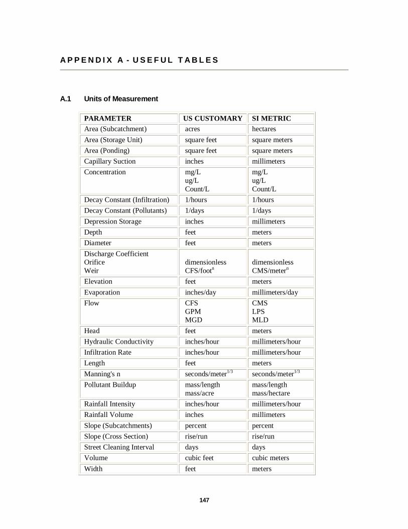
The manual also contains several appendixes: Appendix A - provides several useful tables of parameter values, including a table of units of
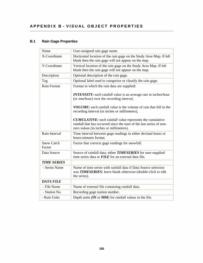
expression for all design and computed parameters. Appendix B - lists the editable properties of all visual objects that can be displayed on the study
area map and be selected for editing using point and click. Appendix C - describes the specialized editors available for setting the properties of non-visual
objects. Appendix D - provides instructions for running the command line version of SWMM and
includes a detailed description of the format of a project file. Appendix E - lists all of the error messages and their meaning that SWMM can produce.
5
(This page intentionally left blank.)
6
C H A P T E R 2 - Q U I C K S T A R T T U T O R I A L
This chapter provides a tutorial on how to use EPA SWMM. If you are not familiar with the elements that comprise a drainage system, and how these are represented in a SWMM model, you might want to review the material in Chapter 3 first.
2.1 Example Study Area
In this tutorial we will model the drainage system serving a 12-acre residential area. The system layout is shown in Figure 2-1 and consists of subcatchment areas3 S1 through S3, storm sewer conduits C1 through C4, and conduit junctions J1 through J4. The system discharges to a creek at the point labeled Out1. We will first go through the steps of creating the objects shown in this diagram on SWMM's study area map and setting the various properties of these objects. Then we will simulate the water quantity and quality response to a 3-inch, 6-hour rainfall event, as well as a continuous, multi-year rainfall record.
Figure 2-1. Example study area.
2.2 Project Setup
Our first task is to create a new SWMM project and make sure that certain default options are selected. Using these defaults will simplify the data entry tasks later on.
1. Launch EPA SWMM if it is not already running and select File >> New from the Main Menu bar to create a new project.
2. Select Project >> Defaults to open the Project Defaults dialog.
3 A subcatchment is an area of land containing a mix of pervious and impervious surfaces whose runoff drains to a common outlet point, which could be either a node of the drainage network or another subcatchment.
7
3. On the ID Labels page of the dialog, set the ID Prefixes as shown in Figure 2-2. This will make SWMM automatically label new objects with consecutive numbers following the designated prefix.
Figure 2-2. Default ID labeling for tutorial example.
4. On the Subcatchments page of the dialog set the following default values: Area 4 Width 400 % Slope 0.5 % Imperv. 50 N-Imperv. 0.01 N-Perv. 0.10 Dstore-Imperv. 0.05 Dstore-Perv 0.05 %Zero-Imperv. 25 Infil. Model <click to edit> - Method Green-Ampt - Suction Head 3.5 - Conductivity 0.5 - Initial Deficit 0.26
8
5. On the Nodes/Links page set the following default values:Node Invert 0 Node Max. Depth 4 Flow Units CFS Conduit Length 400 Conduit Geometry <click to edit>
6. Click OK to accept these choices and close the dialog. If you wanted to save these choices for all future new projects you could check the Save box at the bottom of the form before accepting it.
Next we will set some map display options so that ID labels and symbols will be displayed as we add objects to the study area map, and links will have direction arrows.
1. Select View >> Map Options to bring up the Map Options dialog (see Figure 2-3).
2. Select the Subcatchments page, set the Fill Style to Diagonal and the Symbol Size to 5.
3. Then select the Nodes page and set the Node Size to 5.
4. Select the Annotation page and check off the boxes that will display ID labels for Areas, Nodes, and Links. Leave the others un-checked.
5. Finally, select the Flow Arrows page, select the Filled arrow style, and set the arrow size to 7.
6. Click the OK button to accept these choices and close the dialog.
9
Figure 2-3. Map Options dialog.
Before placing objects on the map we should set its dimensions.
1. Select View >> Dimensions to bring up the Map Dimensions dialog.
2. You can leave the dimensions at their default values for this example.
Finally, look in the status bar at the bottom of the main window and check that the Auto-Length feature is off.
2.3 Drawing Objects
We are now ready to begin adding components to the Study Area Map4. We will start with the subcatchments.
1. Begin by clicking the button on the Object Toolbar. (If the toolbar is not visible then select View >> Toolbars >> Object). Notice how the mouse cursor changes shape to a pencil.
4 Drawing objects on the map is just one way of creating a project. For large projects it might be more convenient to first construct a SWMM project file external to the program. The project file is a text file that describes each object in a specified format as described in Appendix D of this manual. Data extracted from various sources, such as CAD drawings or GIS files, can be used to create the project file.
10
2. Move the mouse to the map location where one of the corners of subcatchment S1 lies and left-click the mouse.
3. Do the same for the next three corners and then right-click the mouse (or hit the Enter key) to close up the rectangle that represents subcatchment S1. You can press the Esc key if instead you wanted to cancel your partially drawn subcatchment and start over again. Don't worry if the shape or position of the object isn't quite right. We will go back later and show how to fix this.
4. Repeat this process for subcatchments S2 and S35.
Observe how sequential ID labels are generated automatically as we add objects to the map.
Next we will add in the junction nodes and the outfall node that comprise part of the drainage network.
1. To begin adding junctions, click the button on the Object Toolbar.
2. Move the mouse to the position of junction J1 and left-click it. Do the same for junctions J2 through J4.
3. To add the outfall node, click the button on the Object Toolbar, move the mouse to the outfall's location on the map, and left-click. Note how the outfall was automatically given the name Out1.
At this point your map should look something like that shown in Figure 2.4.
Figure 2-4. Subcatchments and nodes for example study area.
Now we will add the storm sewer conduits that connect our drainage system nodes to one another. (You must have created a link's end nodes as described previously before you can create the link.) We will begin with conduit C1, which connects junction J1 to J2.
1. Click the button on the Object Toolbar. The mouse cursor changes shape to a crosshair.
2. Click the mouse on junction J1. Note how the mouse cursor changes shape to a pencil.
5 If you right-click (or press Enter) after adding the first point of a subcatchment's outline, the subcatchment will be shown as just a single point.
11
3. Move the mouse over to junction J2 (note how an outline of the conduit is drawn as you move the mouse) and left-click to create the conduit. You could have cancelled the operation by either right clicking or by hitting the <Esc> key.
4. Repeat this procedure for conduits C2 through C4.
Although all of our conduits were drawn as straight lines, it is possible to draw a curved link by left-clicking at intermediate points where the direction of the link changes before clicking on the end node.
To complete the construction of our study area schematic we need to add a rain gage.
1. Click the Rain Gage button on the Object Toolbar.
2. Move the mouse over the Study Area Map to where the gage should be located and left-click the mouse.
At this point we have completed drawing the example study area. Your system should look like the one in Figure 2-1. If a rain gage, subcatchment or node is out of position you can move it by doing the following:
1. If the button is not already depressed, click it to place the map in Object Selection mode.
2. Click on the object to be moved.
3. Drag the object with the left mouse button held down to its new position.
To re-shape a subcatchment's outline:
1. With the map in Object Selection mode, click on the subcatchment's centroid (indicated by a solid square within the subcatchment) to select it.
2. Then click the button on the Map Toolbar to put the map into Vertex Selection mode.
3. Select a vertex point on the subcatchment outline by clicking on it (note how the selected vertex is indicated by a filled solid square).
4. Drag the vertex to its new position with the left mouse button held down.
5. If need be, vertices can be added or deleted from the outline by right-clicking the mouse and selecting the appropriate option from the popup menu that appears.
6. When finished, click the button to return to Object Selection mode.
This same procedure can also be used to re-shape a link.
2.4 Setting Object Properties
As visual objects are added to our project, SWMM assigns them a default set of properties. To change the value of a specific property for an object we must select the object into the Property Editor (see Figure 2-5). There are several different ways to do this. If the Editor is already visible,
12
then you can simply click on the object or select it from the Data page of the Browser Panel of the main window. If the Editor is not visible then you can make it appear by one of the following actions:
� double-click the object on the map,
� or right-click on the object and select Properties from the pop-up menu that appears,
� or select the object from the Data page of the Browser panel and then click the Browser’s button.
Figure 2-5. Property Editor window.
Whenever the Property Editor has the focus you can press the F1 key to obtain a more detailed description of the properties listed.
Two key properties of our subcatchments that need to be set are the rain gage that supplies rainfall data to the subcatchment and the node of the drainage system that receives runoff from the subcatchment. Since all of our subcatchments utilize the same rain gage, Gage1, we can use a shortcut method to set this property for all subcatchments at once:
1. From the main menu select Edit >>Select All.
2. Then select Edit >> Group Edit to make a Group Editor dialog appear (see Figure 2-6).
3. Select Subcatchment as the type of object to edit, Rain Gage as the property to edit, and type in Gage1 as the new value.
4. Click OK to change the rain gage of all subcatchments to Gage1. A confirmation dialog will appear noting that 3 subcatchments have changed. Select “No” when asked to continue editing.
13
Figure 2-6. Group Editor dialog.
Because the outlet nodes vary by subcatchment, we must set them individually as follows:
1. Double click on subcatchment S1 or select it from the Data Browser and click theBrowser's button to bring up the Property Editor.
2. Type J1 in the Outlet field and press Enter. Note how a dotted line is drawn between the subcatchment and the node.
3. Click on subcatchment S2 and enter J2 as its Outlet.
4. Click on subcatchment S3 and enter J3 as its Outlet.
We also wish to represent area S3 as being less developed than the others. Select S3 into the Property Editor and set its % Imperviousness to 25.
The junctions and outfall of our drainage system need to have invert elevations assigned to them. As we did with the subcatchments, select each junction individually into the Property Editor and set its Invert Elevation to the value shown below6.
Node Invert J1 96 J2 90 J3 93 J4 88 Out1 85
Only one of the conduits in our example system has a non-default property value. This is conduit C4, the outlet pipe, whose diameter should be 1.5 instead of 1 ft. To change its diameter:
6 An alternative way to move from one object of a given type to the next in order (or to the previous one) in the Property Editor is to hit the Page Down (or Page Up) key.
14
1. Select conduit C4 into the Property Editor (by either double-clicking anywhere on the conduit itself or by selecting it in the Data Browser and clicking the button).
2. Select the Shape field and click the ellipsis button (or press <Enter>).
3. In the Cross-Section Editor dialog that appears (see Figure 2-7), set the Max. Depth value to 1.5 and then click the OK button.
Figure 2-7. Cross-Section Editor dialog.
In order to provide a source of rainfall input to our project we need to set the rain gage’s properties. Select Gage1 into the Property Editor and set the following properties:
Rain Format INTENSITY Rain Interval 1:00 Data Source TIMESERIES Series Name TS1
As mentioned earlier, we want to simulate the response of our study area to a 3-inch, 6-hour design storm. A time series named TS1 will contain the hourly rainfall intensities that make up this storm. Thus we need to create a time series object and populate it with data. To do this:
1. From the Data Browser select the Time Series category of objects.
2. Click the button on the Browser to bring up the Time Series Editor dialog (see Figure 2-8)7.
3. Enter TS1 in the Time Series Name field.
7 The Time Series Editor can also be launched directly from the Rain Gage Property Editor by selecting the editor's Series Name field and double clicking on it.
15
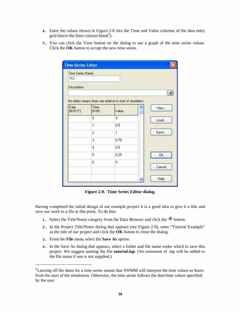
4. Enter the values shown in Figure 2-8 into the Time and Value columns of the data entry grid (leave the Date column blank8).
5. You can click the View button on the dialog to see a graph of the time series values. Click the OK button to accept the new time series.
Figure 2-8. Time Series Editor dialog.
Having completed the initial design of our example project it is a good idea to give it a title and save our work to a file at this point. To do this:
1. Select the Title/Notes category from the Data Browser and click the button.
2. In the Project Title/Notes dialog that appears (see Figure 2-9), enter “Tutorial Example” as the title of our project and click the OK button to close the dialog.
3. From the File menu select the Save As option.
4. In the Save As dialog that appears, select a folder and file name under which to save this project. We suggest naming the file tutorial.inp. (An extension of .inp will be added to the file name if one is not supplied.)
8 Leaving off the dates for a time series means that SWMM will interpret the time values as hours from the start of the simulation. Otherwise, the time series follows the date/time values specified by the user.
16
5. Click Save to save the project to file.
The project data are saved to the file in a readable text format. You can view what the file looks like by selecting Project >> Details from the main menu. To open our project at some later time, you would select the Open command from the File menu.
Figure 2-9. Title/Notes Editor.
2.5 Running a Simulation
Setting Simulation Options
Before analyzing the performance of our example drainage system we need to set some options that determine how the analysis will be carried out. To do this:
1. From the Data Browser, select the Options category and click the button.
2. On the General page of the Simulation Options dialog that appears (see Figure 2-10), select Kinematic Wave as the flow routing method. The flow units should already be set to CFS and the infiltration method to Green-Ampt. The Allow Ponding option should be unchecked.
3. On the Dates page of the dialog, set the End Analysis time to 12:00:00.
4. On the Time Steps page, set the Routing Time Step to 60 seconds.
5. Click OK to close the Simulation Options dialog.
17
Figure 2-10. Simulation Options dialog.
Running a Simulation
We are now ready to run the simulation. To do so, select Project >> Run Simulation (or click
the button). If there was a problem with the simulation, a Status Report will appear describing what errors occurred. Upon successfully completing a run, there are numerous ways in which to view the results of the simulation. We will illustrate just a few here.
Viewing the Status Report
The Status Report contains useful summary information about the results of a simulation run. To view the report, select Report >> Status. A portion of the report for the system just analyzed is shown in Figure 2-11. The full report indicates the following:
� The quality of the simulation is quite good, with negligible mass balance continuity errors for both runoff and routing (-0.23% and 0.03%, respectively, if all data were entered correctly).
18
-------
---------
---------
---------
� Of the 3 inches of rain that fell on the study area, 1.75 infiltrated into the ground and essentially the remainder became runoff.
� The Node Depth Summary table (not shown in Figure 2-11) indicates there was internal flooding in the system at node J29.
� The Conduit Flow Summary table (also not shown in Figure 2-11) shows that Conduit C2, just downstream of node J2, was surcharged and therefore appears to be slightly undersized.
EPA STORM WATER MANAGEMENT MODEL - VERSION 5.0 -----------------------------------------------
Figure 2-11. Portion of the Status Report for initial simulation run.
9 In SWMM, flooding will occur whenever the water surface at a node exceeds the maximum defined depth or if more flow volume enters a node than can be stored or released during a given time step. Normally such water will be lost from the system. The option also exists to have this water pond atop the node and be re-introduced into the drainage system when capacity exists to do so.
19
Viewing Results on the Map
Simulation results (as well as some design parameters, such as subcatchment area, node invert elevation, and link maximum depth) can be viewed in color-coded fashion on the study area map. To view a particular variable in this fashion:
1. Select the Map page of the Browser panel.
2. Select the variables to view for Subcatchments, Nodes, and Links from the dropdown combo boxes appearing in the Themes panel. In Figure 2-12, subcatchment runoff and link flow have been selected for viewing.
3. The color-coding used for a particular variable is displayed with a legend on the study area map. To toggle the display of a legend, select View >> Legends.
4. To move a legend to another location, drag it with the left mouse button held down.
5. To change the color-coding and the breakpoint values for different colors, select View >> Legends >> Modify and then the pertinent class of object (or if the legend is already visible, simply right-click on it). To view numerical values for the variables being displayed on the map, select Tools >> Map Display Options and then select the Annotation page of the Map Options dialog. Use the check boxes for Subcatchment Values, Node Values, and Link Values to specify what kind of annotation to add.
6. The Date / Time / Elapsed Time controls on the Map Browser can be used to move through the simulation results in time. Figure 2-12 depicts results at 5 hours and 45 minutes into the simulation.
7. You can use the controls in the Animator panel of the Map Browser (see Figure 2-12) to animate the map display through time. For example, pressing the button will run the animation forward in time.
Viewing a Time Series Plot
To generate a time series plot of a simulation result:
1. Select Report >> Graph >> Time Series or simply click on the Standard Toolbar.
2. A Time Series Plot dialog will appear. It is used to select the objects and variables to be plotted.
For our example, the Time Series Plot dialog can be used to graph the flow in conduits C1 and C2 as follows (refer to Figure 2-13):
1. Select Links as the Object Category.
2. Select Flow as the Variable to plot.
3. Click on conduit C1 (either on the map or in the Data Browser) and then click in the dialog to add it to the list of links plotted. Do the same for conduit C2.
4. Press OK to create the plot, which should look like the graph in Figure 2-14.
20
Figure 2-12. Example of viewing color-coded results on the Study Area Map.
21
Figure 2-13. Time Series Plot dialog.
Figure 2-14. Time series plot of results from initial simulation run.
22
After a plot is created you can:
� customize its appearance by selecting Report >> Customize or right clicking on the plot,
� copy it to the clipboard and paste it into another application by selecting Edit >> Copy
To or clicking on the Standard Toolbar
� print it by selecting File >> Print or File >> Print Preview (use File >> Page Setup first to set margins, orientation, etc.).
Viewing a Profile Plot
SWMM can generate profile plots showing how water surface depth varies across a path of connected nodes and links. Let's create such a plot for the conduits connecting junction J1 to the outfall Out1 of our example drainage system. To do this:
1.Select Report >> Graph >> Profile or simply click on the Standard Toolbar.
2.Either enter J1 in the Start Node field of the Profile Plot dialog that appears (see Figure 2
15) or select it on the map or from the Data Browser and click the button next to the field.
Figure 2-15. Profile Plot dialog.
3.Do the same for node Out1 in the End Node field of the dialog.
4. Click the Find Path button. An ordered list of the links forming a connected path between the specified Start and End nodes will be displayed in the Links in Profile box. You can edit the entries in this box if need be.
23
5. Click the OK button to create the plot, showing the water surface profile as it exists at the simulation time currently selected in the Map Browser (see Figure 2-16).
Figure 2-16. Example of a profile plot.
As you move through time using the Map Browser or with the Animator control, the water depth profile on the plot will be updated. Observe how node J2 becomes flooded between hours 2 and 3 of the storm event. A Profile Plot’s appearance can be customized and it can be copied or printed using the same procedures as for a Time Series Plot.
Running a Full Dynamic Wave Analysis
In the analysis just run we chose to use the Kinematic Wave method of routing flows through our drainage system. This is an efficient but simplified approach that cannot deal with such phenomena as backwater effects, pressurized flow, flow reversal, and non-dendritic layouts. SWMM also includes a Dynamic Wave routing procedure that can represent these conditions. This procedure, however, requires more computation time, due to the need for smaller time steps to maintain numerical stability.
Most of the effects mentioned above would not apply to our example. However we had one conduit, C2, which flowed full and caused its upstream junction to flood. It could be that this pipe is actually being pressurized and could therefore convey more flow than was computed using Kinematic Wave routing. We would now like to see what would happen if we apply Dynamic Wave routing instead.
24
To run the analysis with Dynamic Wave routing:
1. From the Data Browser, select the Options category and click the button.
2. On the General page of the Simulation Options dialog that appears, select Dynamic Wave as the flow routing method.
3. On the Dynamic Wave page of the dialog, use the settings shown in Figure 2-1710.
Figure 2-17. Dynamic Wave simulation options.
4. Click OK to close the form and select Project >> Run Simulation (or click the button) to re-run the analysis.
10 Normally when running a Dynamic Wave analysis, one would also want to reduce the routing time step (on the Time Steps page of the dialog). In this example, we will continue to use a 1minute time step.
25
If you look at the Status Report for this run, you will see that there is no longer any junction flooding and that the peak flow carried by conduit C2 has been increased from 3.44 cfs to 4.04 cfs.
2.6 Simulating Water Quality
In the next phase of this tutorial we will add water quality analysis to our example project. SWMM has the ability to analyze the buildup, washoff, transport and treatment of any number of water quality constituents. The steps needed to accomplish this are:
1. Identify the pollutants to be analyzed.
2. Define the categories of land uses that generate these pollutants.
3. Set the parameters of buildup and washoff functions that determine the quality of runoff from each land use.
4. Assign a mixture of land uses to each subcatchment area
5. Define pollutant removal functions for nodes within the drainage system that contain treatment facilities.
We will now apply each of these steps, with the exception of number 5, to our example project11.
We will define two runoff pollutants; total suspended solids (TSS), measured as mg/L, and total Lead, measured in ug/L. In addition, we will specify that the concentration of Lead in runoff is a fixed fraction (0.25) of the TSS concentration. To add these pollutants to our project:
1. Under the Quality category in the Data Browser, select the Pollutants sub-category beneath it.
2. Click the button to add a new pollutant to the project.
3. In the Pollutant Editor dialog that appears (see Figure 2-18), enter TSS for the pollutant name and leave the other data fields at their default settings.
4. Click the OK button to close the Editor.
5. Click the button on the Data Browser again to add our next pollutant.
6. In the Pollutant Editor, enter Lead for the pollutant name, select ug/L for the concentration units, enter TSS as the name of the Co-Pollutant, and enter 0.25 as the Co-Fraction value.
7. Click the OK button to close the Editor.
In SWMM, pollutants associated with runoff are generated by specific land uses assigned to subcatchments. In our example, we will define two categories of land uses: Residential and Undeveloped. To add these land uses to the project:
11 Aside from surface runoff, SWMM allows pollutants to be introduced into the nodes of a drainage system through user-defined time series of direct inflows, dry weather inflows, groundwater interflow, and rainfall dependent inflow/infiltration
26
1. Under the Quality category in the Data Browser, select the Land Uses sub-category and click the button.
2. In the Land Use Editor dialog that appears (see Figure 2-19), enter Residential in the Name field and then click the OK button.
3. Repeat steps 1 and 2 to create the Undeveloped land use category.
Figure 2-18. Pollutant Editor dialog. Figure 2-19. Land Use Editor dialog.
Next we need to define buildup and washoff functions for TSS in each of our land use categories. Functions for Lead are not needed since its runoff concentration was defined to be a fixed fraction of the TSS concentration. Normally, defining these functions requires site-specific calibration.
In this example we will assume that suspended solids in Residential areas builds up at a constant rate of 1 pound per acre per day until a limit of 50 lbs per acre is reached. For the Undeveloped area we will assume that buildup is only half as much. For the washoff function, we will assume a constant event mean concentration of 100 mg/L for Residential land and 50 mg/L for Undeveloped land. When runoff occurs, these concentrations will be maintained until the avaliable buildup is exhausted. To define these functions for the Residential land use:
1. Select the Residential land use category from the Data Browser and click the button.
2. In the Land Use Editor dialog, move to the Buildup page (see Figure 2-20).
3. Select TSS as the pollutant and POW (for Power function) as the function type.
27
4. Assign the function a maximum buildup of 50, a rate constant of 1.0, a power of 1 and select AREA as the normalizer.
5. Move to the Washoff page of the dialog and select TSS as the pollutant, EMC as the function type, and enter 100 for the coefficient. Fill the other fields with 0.
6. Click the OK button to accept your entries.
Now do the same for the Undeveloped land use category, except use a maximum buildup of 25, a buildup rate constant of 0.5, a buildup power of 1, and a washoff EMC of 50.
Figure 2-20. Defining a TSS buildup function for Residential land use.
The final step in our water quality example is to assign a mixture of land uses to each subcatchment area:
1. Select subcatchment S1 into the Property Editor.
2. Select the Land Uses property and click the ellipsis button (or press <Enter>).
3. In the Land Use Assignment dialog that appears, enter 75 for the % Residential and 25 for the % Undeveloped (see Figure 2-21). Then click the OK button to close the dialog.
4. Repeat the same three steps for subcatchment S2.
5. Repeat the same for subcatchment S3, except assign the land uses as 25% Residential and 75% Undeveloped.
28
Figure 2-21. Land Use Assignment dialog.
Before we simulate the runoff quantities of TSS and Lead from our study area, an initial buildup of TSS should be defined so it can be washed off during our single rainfall event. We can either specify the number of antecedent dry days prior to the simulation or directly specify the initial buildup mass on each subcatchment. We will use the former method:
1. From the Options category of the Data Browser, select the Dates sub-category and click the button.
2. In the Simulation Options dialog that appears, enter 5 into the Antecedent Dry Days field.
3. Leave the other simulation options the same as they were for the dynamic wave flow routing we just completed.
4. Click the OK button to close the dialog.
Now run the simulation by selecting Project >> Run Simulation or by clicking on the Standard Toolbar.
When the run is completed, view its Status Report. Note that two new sections have been added for Runoff Quality Continuity and Quality Routing Continuity. From the Runoff Quality Continuity table we see that there was an initial buildup of 47.5 lbs of TSS on the study area and an additional 1.9 lbs of buildup added during the dry periods of the simulation. Almost 48 lbs were washed off during the rainfall event. The quantity of Lead washed off is a fixed percentage (25% times 0.001 to convert from mg to ug) of the TSS as was specified.
If you plot the runoff concentration of TSS for subcatchment S1 and S3 together on the same time series graph, as in Figure 2-22, you will see the difference in concentrations resulting from the different mix of land uses in these two areas. You can also see that the duration over which pollutants are washed off is much shorter than the duration of the entire runoff hydrograph (i.e., 1 hour versus about 6 hours). This results from having exhausted the available buildup of TSS over this period of time.
29
Figure 2-22. TSS concentration of runoff from selected subcatchments.
2.7 Running a Continuous Simulation
As a final exercise in this tutorial we will demonstrate how to run a long-term continuous simulation using a historical rainfall record and how to perform a statistical frequency analysis on the results. The rainfall record will come from a file named sta310301.dat that was included with the example data sets provided with EPA SWMM. It contains several years of hourly rainfall beginning in January 1998. The data are stored in the National Climatic Data Center's DSI 3240 format, which SWMM can automatically recognize.
To run a continuous simulation with this rainfall record:
1. Select the rain gage Gage1 into the Property Editor.
2. Change the selection of Data Source to FILE.
3. Select the File Name data field and click the ellipsis button (or press the <Enter> key) to bring up a standard Windows File Selection dialog.
4. Navigate to the folder where the SWMM example files were stored, select the file named sta310301.dat, and click Open to select the file and close the dialog.
5. In the Station No. field of the Property Editor enter 310301.
6. Select the Options category in the Data Browser and click the button to bring up the Simulation Options form.
7. On the General page of the form, select Kinematic Wave as the Routing Method (this will help speed up the computations).
8. On the Date page of the form, set both the Start Analysis and Start Reporting dates to 01/01/1998, and set the End Analysis date to 01/01/2000.
30
9. On the Time Steps page of the form, set the Routing Time Step to 00:05:00.
10.Close the Simulation Options form by clicking the OK button and start the simulation by selecting Project >> Run Simulation (or by clicking on the Standard Toolbar).
After our continuous simulation is completed we can perform a statistical frequency analysis on any of the variables produced as output. For example, to determine the distribution of rainfall volumes within each storm event over the two-year period simulated:
1. Select Report >> Statistics or click the button on the Standard Toolbar.
2. In the Statistics Selection dialog that appears, enter the values shown in Figure 2-23.
3. Click the OK button to close the form.
Figure 2-23. Statistics Selection dialog.
The results of this request will be a Statistics Report form (see Figure 2-24) containing three tabbed pages: a Summary page, an Events page containing a rank-ordered listing of each event, and a Histogram page containing a plot of the occurrence frequency versus event magnitude.
31
Figure 2-24. Statistical Analysis report.
The summary page shows that there were a total of 213 rainfall events. The Events page shows that the largest rainfall event had a volume of 3.35 inches and occurred over a 24- hour period. There were no events that matched the 3-inch, 6-hour design storm event used in our previous single-event analysis that had produced some internal flooding. In fact, the status report for this continuous simulation indicates that there were no flooding or surcharge occurrences over the simulation period.
We have only touched the surface of SWMM's capabilities. Some additional features of the program that you will find useful include:
� utilizing additional types of drainage elements, such as storage units, flow dividers, pumps, and regulators, to model more complex types of systems
� using control rules to simulate real-time operation of pumps and regulators
� employing different types of externally-imposed inflows at drainage system nodes, such as direct time series inflows, dry weather inflows, and rainfall-derived infiltration/inflow
� modeling groundwater interflow between aquifers beneath subcatchment areas and drainage system nodes
� modeling snow fall accumulation and melting within subcatchments
� adding calibration data to a project so that simulated results can be compared with measured values
� utilizing a background street, site plan, or topo map to assist in laying out a system's drainage elements and to help relate simulated results to real-world locations.
You can find more information on these and other features in the remaining chapters of this manual.
32
C H A P T E R 3 - S W M M ‘ s C O N C E P T U A L M O D E L
This chapter discusses how SWMM models the objects and operational parameters that constitute a stormwater drainage system. Details about how this information is entered into the program are presented in later chapters. An overview is also given on the computational methods that SWMM uses to simulate the hydrology, hydraulics and water quality transport behavior of a drainage system.
3.1 Introduction
SWMM conceptualizes a drainage system as a series of water and material flows between several major environmental compartments. These compartments and the SWMM objects they contain include:
� The Atmosphere compartment, from which precipitation falls and pollutants aredeposited onto the land surface compartment. SWMM uses Rain Gage objects torepresent rainfall inputs to the system.
� The Land Surface compartment, which is represented through one or more Subcatchment objects. It receives precipitation from the Atmospheric compartment in the form of rain or snow; it sends outflow in the form of infiltration to the Groundwater compartment and also as surface runoff and pollutant loadings to the Transport compartment.
� The Groundwater compartment receives infiltration from the Land Surface compartment and transfers a portion of this inflow to the Transport compartment. This compartment is modeled using Aquifer objects.
� The Transport compartment contains a network of conveyance elements (channels, pipes, pumps, and regulators) and storage/treatment units that transport water to outfalls or to treatment facilities. Inflows to this compartment can come from surface runoff, groundwater interflow, sanitary dry weather flow, or from user-defined hydrographs. The components of the Transport compartment are modeled with Node and Link objects
Not all compartments need appear in a particular SWMM model. For example, one could model just the transport compartment, using pre-defined hydrographs as inputs.
3.2 Visual Objects
Figure 3-1 depicts how a collection of SWMM’s visual objects might be arranged together to represent a stormwater drainage system. These objects can be displayed on a map in the SWMM workspace. The following sections describe each of these objects.
33
Figure 3-1. Example of physical objects used to model a drainage system.
3.2.1 Rain Gages
Rain Gages supply precipitation data for one or more subcatchment areas in a study region. The rainfall data can be either a user-defined time series or come from an external file. Several different popular rainfall file formats currently in use are supported, as well as a standard user-defined format.
The principal input properties of rain gages include:
� rainfall data type (e.g., intensity, volume, or cumulative volume)
� recording time interval (e.g., hourly, 15-minute, etc.)
� source of rainfall data (input time series or external file)
� name of rainfall data source
3.2.2 Subcatchments
Subcatchments are hydrologic units of land whose topography and drainage system elements direct surface runoff to a single discharge point. The user is responsible for dividing a study area into an appropriate number of subcatchments, and for identifying the outlet point of each subcatchment. Discharge outlet points can be either nodes of the drainage system or other subcatchments.
Subcatchments can be divided into pervious and impervious subareas. Surface runoff can infiltrate into the upper soil zone of the pervious subarea, but not through the impervious subarea. Impervious areas are themselves divided into two subareas - one that contains depression storage and another that does not. Runoff flow from one subarea in a subcatchment can be routed to the other subarea, or both subareas can drain to the subcatchment outlet.
34
Infiltration of rainfall from the pervious area of a subcatchment into the unsaturated upper soil zone can be described using three different models:
� Horton infiltration
� Green-Ampt infiltration
� SCS Curve Number infiltration
To model the accumulation, re-distribution, and melting of precipitation that falls as snow on a subcatchment, it must be assigned a Snow Pack object. To model groundwater flow between an aquifer underneath the subcatchment and a node of the drainage system, the subcatchment must be assigned a set of Groundwater parameters. Pollutant buildup and washoff from subcatchments are associated with the Land Uses assigned to the subcatchment.
The other principal input parameters for subcatchments include:
� assigned rain gage
� outlet node or subcatchment
� assigned land uses
� tributary surface area
� imperviousness
� slope
� characteristic width of overland flow
� Manning's n for overland flow on both pervious and impervious areas
� depression storage in both pervious and impervious areas
� percent of impervious area with no depression storage.
3.2.3 Junction Nodes
Junctions are drainage system nodes where links join together. Physically they can represent the confluence of natural surface channels, manholes in a sewer system, or pipe connection fittings. External inflows can enter the system at junctions. Excess water at a junction can become partially pressurized while connecting conduits are surcharged and can either be lost from the system or be allowed to pond atop the junction and subsequently drain back into the junction.
The principal input parameters for a junction are:
� invert elevation
� height to ground surface
� ponded surface area when flooded (optional)
� external inflow data (optional).
35
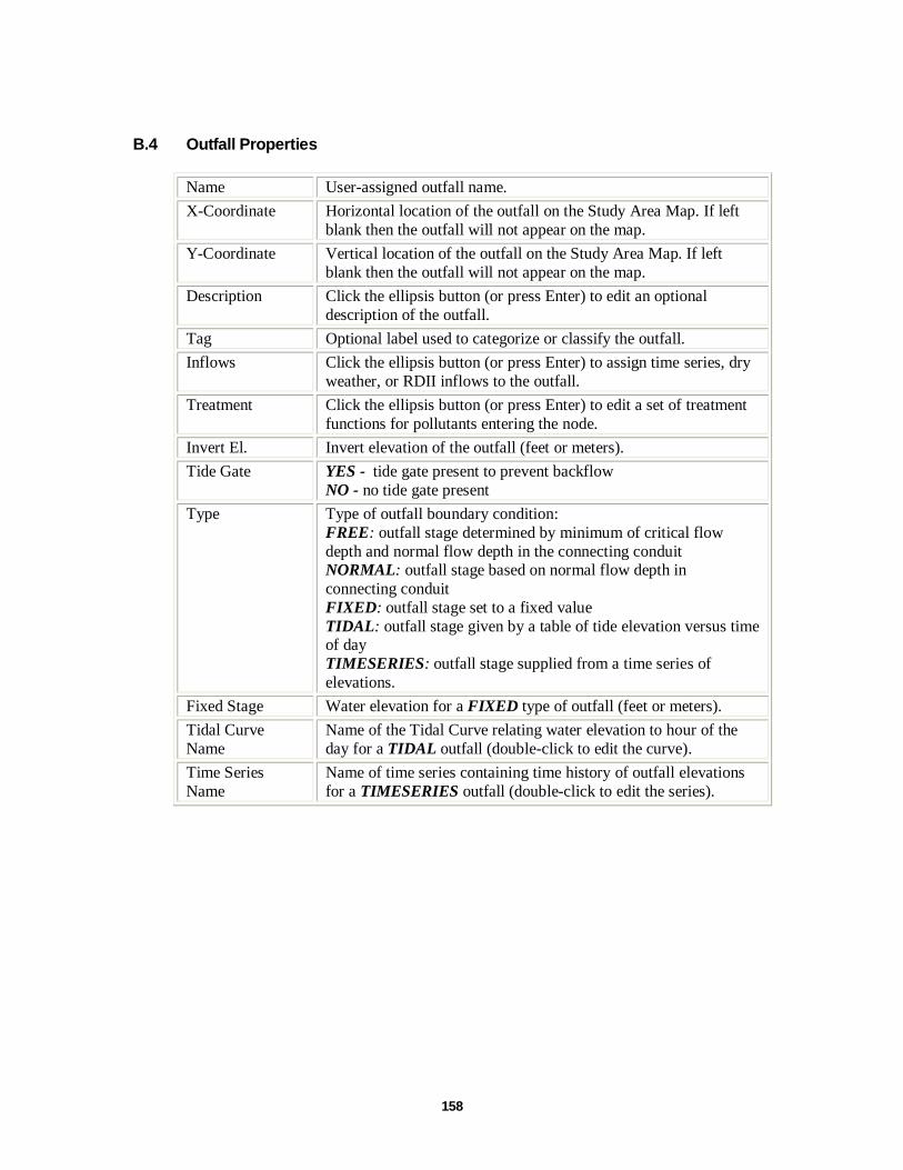
3.2.4 Outfall Nodes
Outfalls are terminal nodes of the drainage system used to define final downstream boundaries under Dynamic Wave flow routing. For other types of flow routing they behave as a junction. Only a single link can be connected to an outfall node.
The boundary conditions at an outfall can be described by any one of the following stage relationships:
� the critical or normal flow depth in the connecting conduit
� a fixed stage elevation
� a tidal stage described in a table of tide height versus hour of the day
� a user-defined time series of stage versus time.
The principal input parameters for outfalls include:
� invert elevation
� boundary condition type and stage description
� presence of a flap gate to prevent backflow through the outfall.
3.2.5 Flow Divider Nodes
Flow Dividers are drainage system nodes that divert inflows to a specific conduit in a prescribed manner. A flow divider can have no more than two conduit links on its discharge side. Flow dividers are only active under Kinematic Wave routing and are treated as simple junctions under Dynamic Wave routing.
There are four types of flow dividers, defined by the manner in which inflows are diverted:
Cutoff Divider: diverts all inflow above a defined cutoff value.Overflow Divider: diverts all inflow above the flow capacity of the non-diverted
conduit.Tabular Divider: uses a table that expresses diverted flow as a function of total
inflow.Weir Divider: uses a weir equation to compute diverted flow.
The flow diverted through a weir divider is computed by the following equation
) 5.1 Q = C ( fHdiv w w
where Qdiv = diverted flow, Cw = weir coefficient, Hw = weir height and f is computed as
Q − Qin minf = Q − Qmax min
where Qin is the inflow to the divider, Qmin is the flow at which diversion begins, and 5.1 = H C Qmax w w . The user-specified parameters for the weir divider are Qmin, Hw, and Cw.
36
The principal input parameters for a flow divider are:
� junction parameters (see above)
� name of the link receiving the diverted flow
� method used for computing the amount of diverted flow.
3.2.6 Storage Units
Storage Units are drainage system nodes that provide storage volume. Physically they could represent storage facilities as small as a catch basin or as large as a lake. The volumetric properties of a storage unit are described by a function or table of surface area versus height.
The principal input parameters for storage units include:
� invert elevation
� maximum depth
� depth-surface area data
� evaporation potential
� ponded surface area when flooded (optional)
� external inflow data (optional).
3.2.7 Conduits
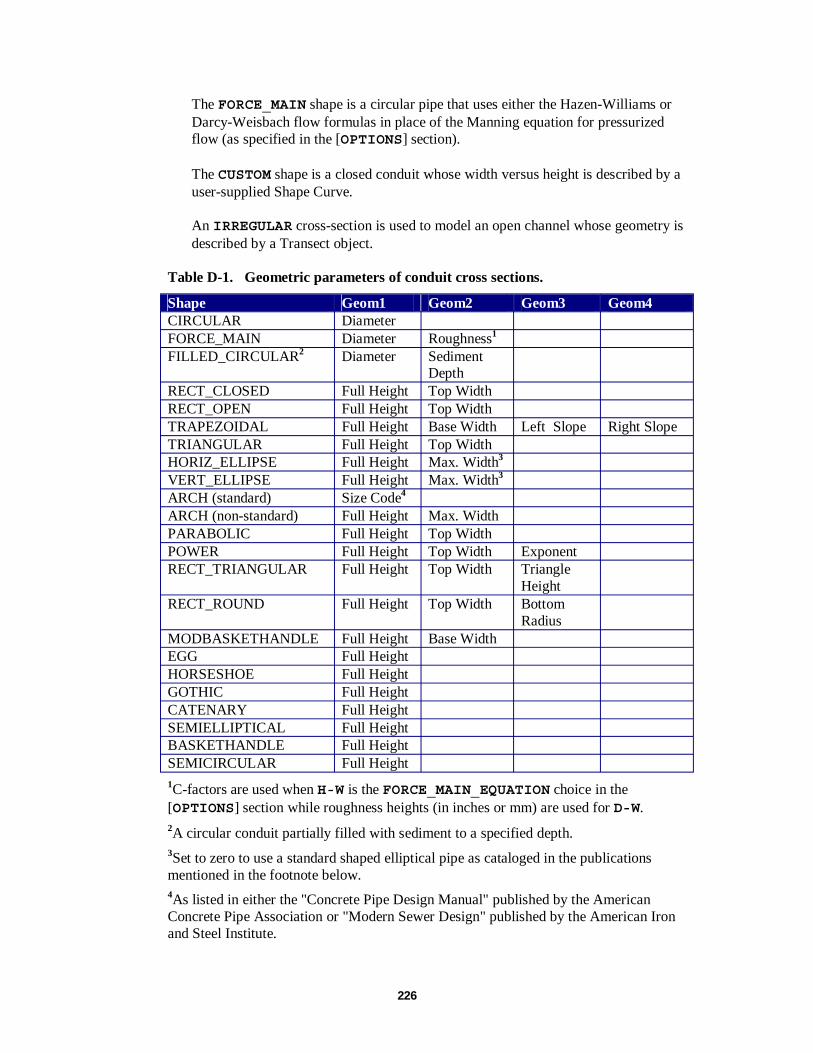
Conduits are pipes or channels that move water from one node to another in the conveyance system. Their cross-sectional shapes can be selected from a variety of standard open and closed geometries as listed in Table 3-1.
Most open channels can be represented with a rectangular, trapezoidal, or user-defined irregular cross-section shape. For the latter, a Transect object is used to define how depth varies with distance across the cross-section (see Section 3.3.5 below). The most common shapes for new drainage and sewer pipes are circular, elliptical, and arch pipes. They come in standard sizes that are published by the American Iron and Steel Institute in Modern Sewer Design and by the American Concrete Pipe Association in the Concrete Pipe Design Manual. The Filled Circular shape allows the bottom of a circular pipe to be filled with sediment and thus limit its flow capacity. The Custom Closed Shape allows any closed geometrical shape that is symmetrical about the center line to be defined by supplying a Shape Curve for the cross section (see Section 3.3.11 below).
37
Table 3-1. Available cross section shapes for conduits Name Parameters Shape Name Parameters Shape Circular Full Height Circular Force Full Height,
Main Roughness
Filled Full Height, Rectangular Full Height, Circular Filled Depth Closed Width
Rectangular – Full Height, Trapezoidal Full Height, Open Width Base Width,
Side Slopes
Triangular Full Height, Horizontal Full Height, Top Width Ellipse Max. Width
Vertical Full Height, Arch Full Height, Ellipse Max. Width Max. Width
Parabolic Full Height, Power Full Height, Top Width Top Width,
Exponent
Rectangular- Full Height, Rectangular- Full Height, Triangular Top Width, Round Top Width,
Triangle Bottom Height Radius
Modified Full Height, Egg Full Height Baskethandle Top Width
Horseshoe Full Height Gothic Full Height
Catenary Full Height Semi-Elliptical
Full Height
Baskethandle Full Height Semi-Circular Full Height
SWMM uses the Manning equation to express the relationship between flow rate (Q), cross-sectional area (A), hydraulic radius (R), and slope (S) in all conduits. For standard U.S. units,
1.49 2/3S 1/2Q = AR n
where n is the Manning roughness coefficient. The slope S is interpreted as either the conduit slope or the friction slope (i.e., head loss per unit length), depending on the flow routing method used.
For pipes with Circular Force Main cross-sections either the Hazen-Williams or Darcy-Weisbach formula is used in place of the Manning equation for fully pressurized flow. For U.S. units the Hazen-Williams formula is:
63 0 S 54 0 . .Q = R A C 1.318
where C is the Hazen-Williams C-factor which varies inversely with surface roughness and is supplied as one of the cross-section’s parameters. The Darcy-Weisbach formula is:
1/2S 1/2Q = 8g ARf
where g is the acceleration of gravity and f is the Darcy-Weisbach friction factor. For turbulent flow, the latter is determined from the height of the roughness elements on the walls of the pipe (supplied as an input parameter) and the flow’s Reynolds Number using the Colebrook-White equation. The choice of which equation to use is a user-supplied option.
A conduit does not have to be assigned a Force Main shape for it to pressurize. Any of the closed cross-section shapes can potentially pressurize and thus function as force mains that use the Manning equation to compute friction losses.
The principal input parameters for conduits are:
� names of the inlet and outlet nodes
� offset heights of the conduit above the inlet and outlet node inverts
� conduit length
� Manning's roughness
� cross-sectional geometry
� entrance/exit losses (optional)
� presence of a flap gate to prevent reverse flow (optional).
39
3.2.8 Pumps
Pumps are links used to lift water to higher elevations. A pump curve describes the relation between a pump's flow rate and conditions at its inlet and outlet nodes. Four different types of pump curves are supported:
Type1 An off-line pump with a wet well where flow increases incrementally with available wet well volume
Type2 An in-line pump where flow increases incrementally with inlet node depth.
Type3 An in-line pump where flow varies continuously with head difference between the inlet and outlet nodes.
Type4 A variable speed in-line pump where flow varies continuously with inlet node depth.
Ideal An "ideal" transfer pump whose flow rate equals the inflow rate at its inlet node. No curve is required. The pump must be the only outflow link from its inlet node. Used mainly for preliminary design.
The on/off status of pumps can be controlled dynamically by specifying startup and shutoff water depths at the inlet node or through user-defined Control Rules. Rules can also be used to simulate variable speed drives that modulate pump flow.
The principal input parameters for a pump include:
� names of its inlet and outlet nodes
� name of its pump curve
40
� initial on/off status
� startup and shutoff depths.
3.2.9 Flow Regulators
Flow Regulators are structures or devices used to control and divert flows within a conveyance system. They are typically used to:
� control releases from storage facilities
� prevent unacceptable surcharging
� divert flow to treatment facilities and interceptors
SWMM can model the following types of flow regulators: Orifices, Weirs, and Outlets.
Orifices
Orifices are used to model outlet and diversion structures in drainage systems, which are typically openings in the wall of a manhole, storage facility, or control gate. They are internally represented in SWMM as a link connecting two nodes. An orifice can have either a circular or rectangular shape, be located either at the bottom or along the side of the upstream node, and have a flap gate to prevent backflow.
Orifices can be used as storage unit outlets under all types of flow routing. If not attached to a storage unit node, they can only be used in drainage networks that are analyzed with Dynamic Wave flow routing.
The flow through a fully submerged orifice is computed as
Q = CA 2gh
where Q = flow rate, C = discharge coefficient, A = area of orifice opening, g = acceleration of gravity, and h = head difference across the orifice. The height of an orifice's opening can be controlled dynamically through user-defined Control Rules. This feature can be used to model gate openings and closings.
The principal input parameters for an orifice include:
� names of its inlet and outlet nodes
� configuration (bottom or side)
� shape (circular or rectangular)
� height above the inlet node invert
� discharge coefficient
� time to open or close.
41
Weirs
Weirs, like orifices, are used to model outlet and diversion structures in a drainage system. Weirs are typically located in a manhole, along the side of a channel, or within a storage unit. They are internally represented in SWMM as a link connecting two nodes, where the weir itself is placed at the upstream node. A flap gate can be included to prevent backflow.
Four varieties of weirs are available, each incorporating a different formula for computing flow across the weir as listed in Table 3-2.
Table 3-2. Available types of weirs.
Weir Type Cross Section Shape Flow Formula Transverse Rectangular 2/Lh C 3
w
Side flow Rectangular 3/Lh C 5 w
V-notch Triangular 2/Sh C 5 w
Trapezoidal Trapezoidal /52/3 ShCLh C wsw + 2
Cw = weir discharge coefficient, L = weir length, S = side slope of V-notch or trapezoidal weir, h = head difference across the weir, Cws = discharge coefficient through sides of trapezoidal weir.
Weirs can be used as storage unit outlets under all types of flow routing. If not attached to a storage unit, they can only be used in drainage networks that are analyzed with Dynamic Wave flow routing.
The height of the weir crest above the inlet node invert can be controlled dynamically through user-defined Control Rules. This feature can be used to model inflatable dams.
The principal input parameters for a weir include:
� names of its inlet and outlet nodes
� shape and geometry
� crest height above the inlet node invert
� discharge coefficient.
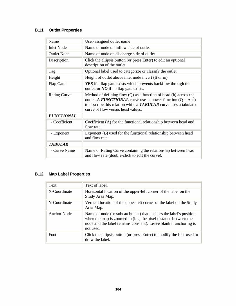
Outlets
Outlets are flow control devices that are typically used to control outflows from storage units. They are used to model special head-discharge relationships that cannot be characterized by pumps, orifices, or weirs. Outlets are internally represented in SWMM as a link connecting two nodes. An outlet can also have a flap gate that restricts flow to only one direction.
Outlets attached to storage units are active under all types of flow routing. If not attached to a storage unit, they can only be used in drainage networks analyzed with Dynamic Wave flow routing.
42
A user-defined rating curve determines an outlet's discharge flow as a function of the head difference across it. Control Rules can be used to dynamically adjust this flow when certain conditions exist.
The principal input parameters for an outlet include:
� names of its inlet and outlet nodes
� height above the inlet node invert
� function or table containing its head-discharge relationship.
3.2.10 Map Labels
Map Labels are optional text labels added to SWMM's Study Area Map to help identify particular objects or regions of the map. The labels can be drawn in any Windows font, freely edited and be dragged to any position on the map.
3.3 Non-Visual Objects
In addition to physical objects that can be displayed visually on a map, SWMM utilizes several classes of non-visual data objects to describe additional characteristics and processes within a study area.
3.3.1 Climatology
Temperature
Air temperature data are used when simulating snowfall and snowmelt processes during runoff calculations. If these processes are not being simulated then temperature data are not required. Air temperature data can be supplied to SWMM from one of the following sources:
� a user-defined time series of point values (values at intermediate times are interpolated)
� an external climate file containing daily minimum and maximum values (SWMM fits a sinusoidal curve through these values depending on the day of the year).
For user-defined time series, temperatures are in degrees F for US units and degrees C for metric units. The external climate file can also be used to supply evaporation and wind speed as well.
Evaporation
Evaporation can occur for standing water on subcatchment surfaces, for subsurface water in groundwater aquifers, and for water held in storage units. Evaporation rates can be stated as:
� a single constant value
� a set of monthly average values
� a user-defined time series of daily values
� daily values read from an external climate file.
43
If a climate file is used, then a set of monthly pan coefficients should also be supplied to convert the pan evaporation data to free water-surface values.
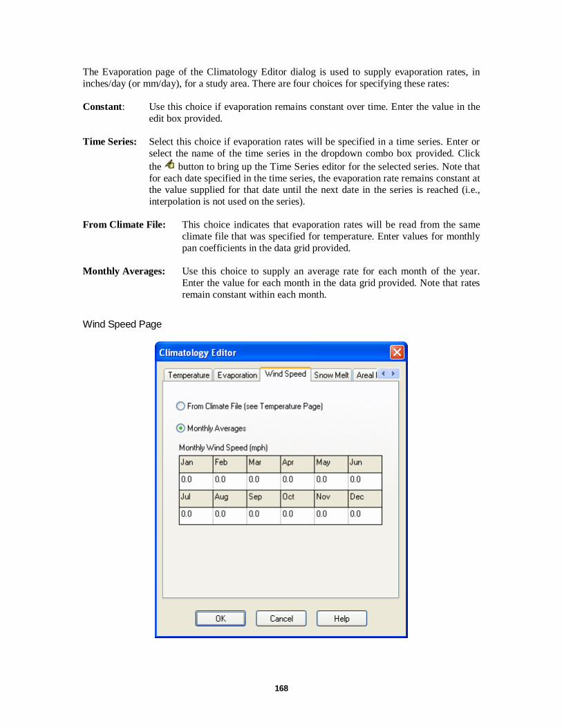
Wind Speed
Wind speed is an optional climatic variable that is only used for snowmelt calculations. SWMM can use either a set of monthly average speeds or wind speed data contained in the same climate file used for daily minimum/maximum temperatures.
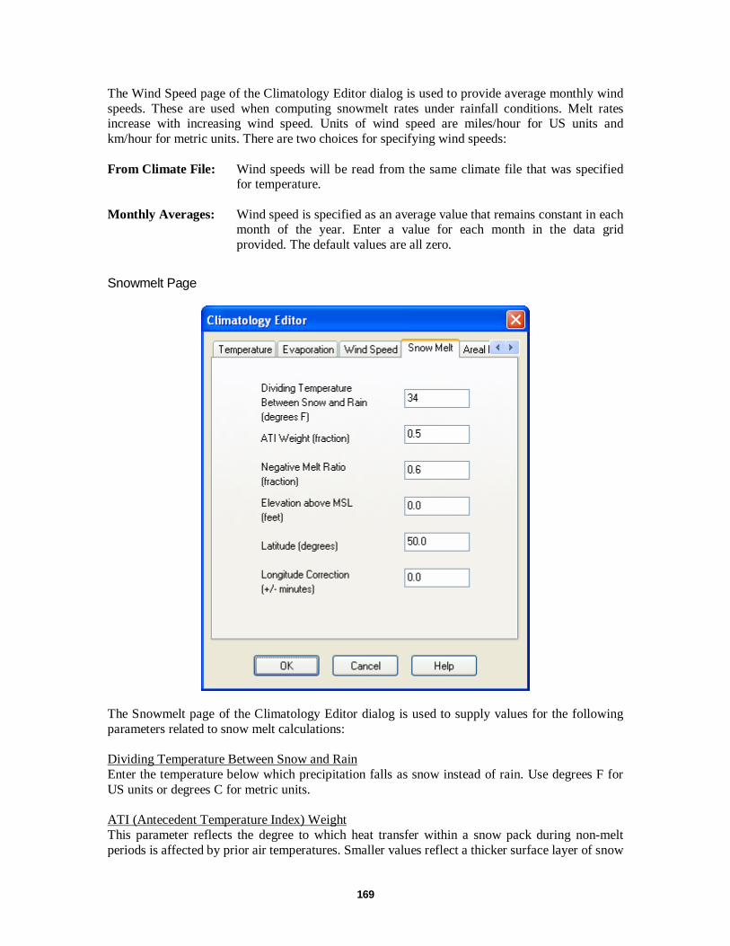
Snowmelt
Snowmelt parameters are climatic variables that apply across the entire study area when simulating snowfall and snowmelt. They include:
� the air temperature at which precipitation falls as snow
� heat exchange properties of the snow surface
� study area elevation, latitude, and longitude correction
Areal Depletion
Areal depletion refers to the tendency of accumulated snow to melt non-uniformly over the surface of a subcatchment. As the melting process proceeds, the area covered by snow gets reduced. This behavior is described by an Areal Depletion Curve that plots the fraction of total area that remains snow covered against the ratio of the actual snow depth to the depth at which there is 100% snow cover. A typical ADC for a natural area is shown in Figure 3-2. Two such curves can be supplied to SWMM, one for impervious areas and another for pervious areas.
Figure 3-2. Areal Depletion curve for a natural area.
3.3.2 Snow Packs
Snow Pack objects contain parameters that characterize the buildup, removal, and melting of snow over three types of sub-areas within a subcatchment:
� The Plowable snow pack area consists of a user-defined fraction of the total impervious area. It is meant to represent such areas as streets and parking lots where plowing and snow removal can be done.
44
� The Impervious snow pack area covers the remaining impervious area of a subcatchment.
� The Pervious snow pack area encompasses the entire pervious area of a subcatchment.
Each of these three areas is characterized by the following parameters:
� Minimum and maximum snow melt coefficients
� minimum air temperature for snow melt to occur
� snow depth above which 100% areal coverage occurs
� initial snow depth
� initial and maximum free water content in the pack.
In addition, a set of snow removal parameters can be assigned to the Plowable area. These parameters consist of the depth at which snow removal begins and the fractions of snow moved onto various other areas.
Subcatchments are assigned a snow pack object through their Snow Pack property. A single snow pack object can be applied to any number of subcatchments. Assigning a snow pack to a subcatchment simply establishes the melt parameters and initial snow conditions for that subcatchment. Internally, SWMM creates a "physical" snow pack for each subcatchment, which tracks snow accumulation and melting for that particular subcatchment based on its snow pack parameters, its amount of pervious and impervious area, and the precipitation history it sees.
3.3.3 Aquifers
Aquifers are sub-surface groundwater areas used to model the vertical movement of water infiltrating from the subcatchments that lie above them. They also permit the infiltration of groundwater into the drainage system, or exfiltration of surface water from the drainage system, depending on the hydraulic gradient that exists. The same aquifer object can be shared by several subcatchments. Aquifers are only required in models that need to explicitly account for the exchange of groundwater with the drainage system or to establish baseflow and recession curves in natural channels and non-urban systems.
Aquifers are represented using two zones – an un-saturated zone and a saturated zone. Their behavior is characterized using such parameters as soil porosity, hydraulic conductivity, evapotranspiration depth, bottom elevation, and loss rate to deep groundwater. In addition, the initial water table elevation and initial moisture content of the unsaturated zone must be supplied.
Aquifers are connected to subcatchments and to drainage system nodes as defined in a subcatchment's Groundwater Flow property. This property also contains parameters that govern the rate of groundwater flow between the aquifer's saturated zone and the drainage system node.
3.3.4 Unit Hydrographs
Unit Hydrographs (UHs) estimate rainfall-derived infiltration/inflow (RDII) into a sewer system. A UH set contains up to three such hydrographs, one for a short-term response, one for an intermediate-term response, and one for a long-term response. A UH group can have up to 12 UH sets, one for each month of the year. Each UH group is considered as a separate object by
45
SWMM, and is assigned its own unique name along with the name of the rain gage that supplies rainfall data to it.
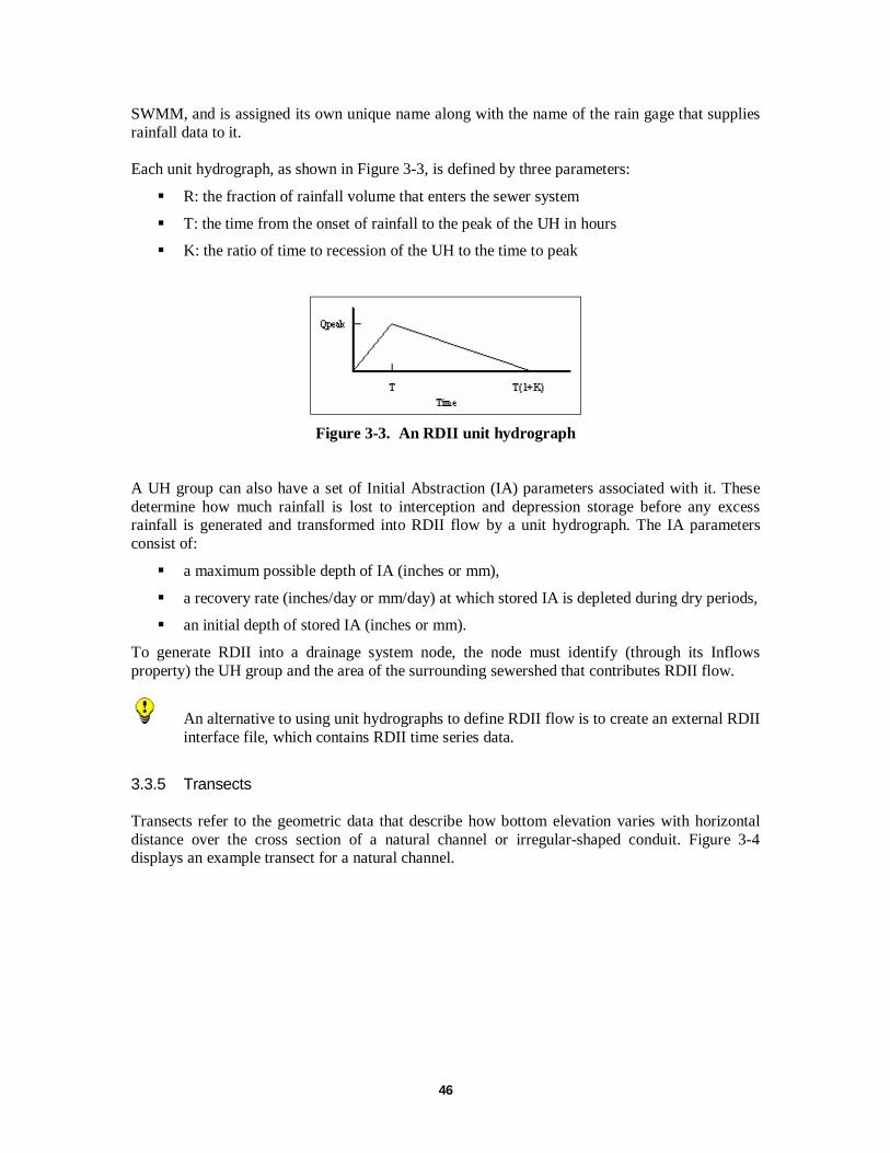
Each unit hydrograph, as shown in Figure 3-3, is defined by three parameters:
� R: the fraction of rainfall volume that enters the sewer system
� T: the time from the onset of rainfall to the peak of the UH in hours
� K: the ratio of time to recession of the UH to the time to peak
Figure 3-3. An RDII unit hydrograph
A UH group can also have a set of Initial Abstraction (IA) parameters associated with it. These determine how much rainfall is lost to interception and depression storage before any excess rainfall is generated and transformed into RDII flow by a unit hydrograph. The IA parameters consist of:
� a maximum possible depth of IA (inches or mm),
� a recovery rate (inches/day or mm/day) at which stored IA is depleted during dry periods,
� an initial depth of stored IA (inches or mm).
To generate RDII into a drainage system node, the node must identify (through its Inflows property) the UH group and the area of the surrounding sewershed that contributes RDII flow.
An alternative to using unit hydrographs to define RDII flow is to create an external RDII interface file, which contains RDII time series data.
3.3.5 Transects
Transects refer to the geometric data that describe how bottom elevation varies with horizontal distance over the cross section of a natural channel or irregular-shaped conduit. Figure 3-4 displays an example transect for a natural channel.
46
Figure 3-4. Example of a natural channel transect.
Each transect must be given a unique name. Conduits refer to that name to represent their shape. A special Transect Editor is available for editing the station-elevation data of a transect. SWMM internally converts these data into tables of area, top width, and hydraulic radius versus channel depth. In addition, as shown in the diagram above, each transect can have a left and right overbank section whose Manning's roughness can be different from that of the main channel. This feature can provide more realistic estimates of channel conveyance under high flow conditions.
3.3.6 External Inflows
In addition to inflows originating from subcatchment runoff and groundwater, drainage system nodes can receive three other types of external inflows:
� Direct Inflows - These are user-defined time series of inflows added directly into a node. They can be used to perform flow and water quality routing in the absence of any runoff computations (as in a study area where no subcatchments are defined).
� Dry Weather Inflows - These are continuous inflows that typically reflect the contribution from sanitary sewage in sewer systems or base flows in pipes and stream channels. They are represented by an average inflow rate that can be periodically adjusted on a monthly, daily, and hourly basis by applying Time Pattern multipliers to this average value.
� Rainfall-Dependent Infiltration/Inflow (RDII) - These are stormwater flows that enter sanitary or combined sewers due to "inflow" from direct connections of downspouts, sump pumps, foundation drains, etc. as well as "infiltration" of subsurface water through cracked pipes, leaky joints, poor manhole connections, etc. RDII can be computed for a given rainfall record based on set of triangular unit hydrographs (UH) that determine a short-term, intermediate-term, and long-term inflow response for each time period of rainfall. Any number of UH sets can be supplied for different sewershed areas and different months of the year. RDII flows can also be specified in an external RDII interface file.
Direct, Dry Weather, and RDII inflows are properties associated with each type of drainage system node (junctions, outfalls, flow dividers, and storage units) and can be specified when
47
nodes are edited. It is also possible to make the outflows generated from an upstream drainage system be the inflows to a downstream system by using interface files. See Section 11.7 for further details.
3.3.7 Control Rules
Control Rules determine how pumps and regulators in the drainage system will be adjusted over the course of a simulation. Some examples of these rules are:
Simple time-based pump control:
RULE R1 IF SIMULATION TIME > 8 THEN PUMP 12 STATUS = ON ELSE PUMP 12 STATUS = OFF
Multiple-condition orifice gate control:
RULE R2A IF NODE 23 DEPTH > 12 AND LINK 165 FLOW > 100 THEN ORIFICE R55 SETTING = 0.5
RULE R2B IF NODE 23 DEPTH > 12 AND LINK 165 FLOW > 200 THEN ORIFICE R55 SETTING = 1.0
RULE R2C IF NODE 23 DEPTH <= 12 OR LINK 165 FLOW <= 100 THEN ORIFICE R55 SETTING = 0
Pump station operation:
RULE R3A IF NODE N1 DEPTH > 5 THEN PUMP N1A STATUS = ON
RULE R3B IF NODE N1 DEPTH > 7 THEN PUMP N1B STATUS = ON
RULE R3C IF NODE N1 DEPTH <= 3 THEN PUMP N1A STATUS = OFF AND PUMP N1B STATUS = OFF
48
Modulated weir height control:
RULE R4 IF NODE N2 DEPTH >= 0 THEN WEIR W25 SETTING = CURVE C25
Appendix C.3 describes the control rule format in more detail and the special Editor used to edit them.
3.3.8 Pollutants
SWMM can simulate the generation, inflow and transport of any number of user-defined pollutants. Required information for each pollutant includes:
� pollutant name
� concentration units (i.e., milligrams/liter, micrograms/liter, or counts/liter)
� concentration in rainfall
� concentration in groundwater
� concentration in direct infiltration/inflow
� first-order decay coefficient.
Co-pollutants can also be defined in SWMM. For example, pollutant X can have a co-pollutant Y, meaning that the runoff concentration of X will have some fixed fraction of the runoff concentration of Y added to it.
Pollutant buildup and washoff from subcatchment areas are determined by the land uses assigned to those areas. Input loadings of pollutants to the drainage system can also originate from external time series inflows as well as from dry weather inflows.
3.3.9 Land Uses
Land Uses are categories of development activities or land surface characteristics assigned to subcatchments. Examples of land use activities are residential, commercial, industrial, and undeveloped. Land surface characteristics might include rooftops, lawns, paved roads, undisturbed soils, etc. Land uses are used solely to account for spatial variation in pollutant buildup and washoff rates within subcatchments.
The SWMM user has many options for defining land uses and assigning them to subcatchment areas. One approach is to assign a mix of land uses for each subcatchment, which results in all land uses within the subcatchment having the same pervious and impervious characteristics. Another approach is to create subcatchments that have a single land use classification along with a distinct set of pervious and impervious characteristics that reflects the classification.
49
The following processes can be defined for each land use category:
� pollutant buildup
� pollutant washoff
� street cleaning.
Pollutant Buildup
Pollutant buildup that accumulates within a land use category is described (or “normalized”) by either a mass per unit of subcatchment area or per unit of curb length. Mass is expressed in pounds for US units and kilograms for metric units. The amount of buildup is a function of the number of preceding dry weather days and can be computed using one of the following functions:
Power Function: Pollutant buildup (B) accumulates proportionally to time (t) raised to some power, until a maximum limit is achieved,
( 1B = t C, C Min C3 )2
where C1 = maximum buildup possible (mass per unit of area or curb length), C2 = buildup rate constant, and C3 = time exponent.
Exponential Function: Buildup follows an exponential growth curve that approaches a maximum limit asymptotically,
− t C )2B = C1 (1− e
where C1 = maximum buildup possible (mass per unit of area or curb length) and C2 = buildup rate constant (1/days).
Saturation Function: Buildup begins at a linear rate that continuously declines with time until a saturation value is reached,
t C 1B = C2 + t
where C1 = maximum buildup possible (mass per unit area or curb length) and C2 = half-saturation constant (days to reach half of the maximum buildup).
Pollutant Washoff
Pollutant washoff from a given land use category occurs during wet weather periods and can be described in one of the following ways:
Exponential Washoff: The washoff load (W) in units of mass per hour is proportional to the product of runoff raised to some power and to the amount of buildup remaining,
W = q C C2 B1
50
where C1 = washoff coefficient, C2 = washoff exponent, q = runoff rate per unit area (inches/hour or mm/hour), and B = pollutant buildup in mass (lbs or kg) per unit area or curb length. Washoff mass units are the same as used to express the pollutant's concentration (milligrams, micrograms, or counts).
Rating Curve Washoff: The rate of washoff W in mass per second is proportional to the runoff rate raised to some power,
2W = Q C C 1
where C1 = washoff coefficient, C2 = washoff exponent, and Q = runoff rate in user-defined flow units.
Event Mean Concentration: This is a special case of Rating Curve Washoff where the exponent is 1.0 and the coefficient C1 represents the washoff pollutant concentration in mass per liter (Note: the conversion between user-defined flow units used for runoff and liters is handled internally by SWMM).
Note that in each case buildup is continuously depleted as washoff proceeds, and washoff ceases when there is no more buildup available.
Washoff loads for a given pollutant and land use category can be reduced by a fixed percentage by specifying a BMP Removal Efficiency that reflects the effectiveness of any BMP controls associated with the land use. It is also possible to use the Event Mean Concentration option by itself, without having to model any pollutant buildup at all.
Street Sweeping
Street sweeping can be used on each land use category to periodically reduce the accumulated buildup of specific pollutants. The parameters that describe street sweeping include:
� days between sweeping
� days since the last sweeping at the start of the simulation
� the fraction of buildup of all pollutants that is available for removal by sweeping
� the fraction of available buildup for each pollutant removed by sweeping
Note that these parameters can be different for each land use, and the last parameter can vary also with pollutant.
3.3.10 Treatment
Removal of pollutants from the flow streams entering any drainage system node is modeled by assigning a set of treatment functions to the node. A treatment function can be any well-formed mathematical expression involving:
� the pollutant concentration of the mixture of all flow streams entering the node (use the pollutant name to represent a concentration)
� the removals of other pollutants (use R_ prefixed to the pollutant name to represent removal)
51
� any of the following process variables: - FLOW for flow rate into node (in user-defined flow units) - DEPTH for water depth above node invert (ft or m)
2- AREA for node surface area (ft2 or m ) - DT for routing time step (sec) - HRT for hydraulic residence time (hours)
The result of the treatment function can be either a concentration (denoted by the letter C) or a fractional removal (denoted by R). For example, a first-order decay expression for BOD exiting from a storage node might be expressed as:
C = BOD * exp(-0.05*HRT)
or the removal of some trace pollutant that is proportional to the removal of total suspended solids (TSS) could be expressed as:
R = 0.75 * R_TSS
3.3.11 Curves
Curve objects are used to describe a functional relationship between two quantities. The following types of curves are available in SWMM:
� Storage - describes how the surface area of a Storage Unit node varies with water depth.
� Shape - describes how the width of a customized cross-sectional shape varies with height for a Conduit link.
� Diversion - relates diverted outflow to total inflow for a Flow Divider node.
� Tidal - describes how the stage at an Outfall node changes by hour of the day.
� Pump - relates flow through a Pump link to the depth or volume at the upstream node or to the head delivered by the pump.
� Rating - relates flow through an Outlet link to the head difference across the outlet.
� Control - determines how the control setting of a pump or flow regulator varies as a function of some control variable (such as water level at a particular node) as specified in a Modulated Control rule.
Each curve must be given a unique name and can be assigned any number of data pairs.
3.3.12 Time Series
Time Series objects are used to describe how certain object properties vary with time. Time series can be used to describe:
� temperature data
� evaporation data
� rainfall data
� water stage at outfall nodes
52
� external inflow hydrographs at drainage system nodes
� external inflow pollutographs at drainage system nodes
� control settings for pumps and flow regulators..
Each time series must be given a unique name and can be assigned any number of time-value data pairs. Time can be specified either as hours from the start of a simulation or as an absolute date and time-of-day.
For rainfall time series, it is only necessary to enter periods with non-zero rainfall amounts. SWMM interprets the rainfall value as a constant value lasting over the recording interval specified for the rain gage that utilizes the time series. For all other types of time series, SWMM uses interpolation to estimate values at times that fall in between the recorded values.
For times that fall outside the range of the time series, SWMM will use a value of 0 for rainfall and external inflow time series, and either the first or last series value for temperature, evaporation, and water stage time series.
3.3.13 Time Patterns
Time Patterns allow external Dry Weather Flow (DWF) to vary in a periodic fashion. They consist of a set of adjustment factors applied as multipliers to a baseline DWF flow rate or pollutant concentration. The different types of time patterns include:
Monthly - one multiplier for each month of the year
Daily - one multiplier for each day of the week
Hourly - one multiplier for each hour from 12 AM to 11 PM
Weekend - hourly multipliers for weekend days
Each Time Pattern must have a unique name and there is no limit on the number of patterns that can be created. Each dry weather inflow (either flow or quality) can have up to four patterns associated with it, one for each type listed above.
3.4 Computational Methods
SWMM is a physically based, discrete-time simulation model. It employs principles of conservation of mass, energy, and momentum wherever appropriate. This section briefly describes the methods SWMM uses to model stormwater runoff quantity and quality through the following physical processes:
The conceptual view of surface runoff used by SWMM is illustrated in Figure 3-5 below. Each subcatchment surface is treated as a nonlinear reservoir. Inflow comes from precipitation and any designated upstream subcatchments. There are several outflows, including infiltration, evaporation, and surface runoff. The capacity of this "reservoir" is the maximum depression storage, which is the maximum surface storage provided by ponding, surface wetting, and interception. Surface runoff per unit area, Q, occurs only when the depth of water in the "reservoir" exceeds the maximum depression storage, dp, in which case the outflow is given by Manning's equation. Depth of water over the subcatchment (d in feet) is continuously updated with time (t in seconds) by solving numerically a water balance equation over the subcatchment.
Figure 3-5. Conceptual view of surface runoff.
3.4.2 Infiltration
Infiltration is the process of rainfall penetrating the ground surface into the unsaturated soil zone of pervious subcatchments areas. SWMM offers three choices for modeling infiltration:
Horton's Equation This method is based on empirical observations showing that infiltration decreases exponentially from an initial maximum rate to some minimum rate over the course of a long rainfall event. Input parameters required by this method include the maximum and minimum infiltration rates, a decay coefficient that describes how fast the rate decreases over time, and a time it takes a fully saturated soil to completely dry.
Green-Ampt Method This method for modeling infiltration assumes that a sharp wetting front exists in the soil column, separating soil with some initial moisture content below from saturated soil above. The input parameters required are the initial moisture deficit of the soil, the soil's hydraulic conductivity, and the suction head at the wetting front.
Curve Number Method This approach is adopted from the NRCS (SCS) Curve Number method for estimating runoff. It assumes that the total infiltration capacity of a soil can be found from the soil's tabulated Curve Number. During a rain event this capacity is depleted as a function of cumulative rainfall and
54
remaining capacity. The input parameters for this method are the curve number, the soil's hydraulic conductivity (used to estimate a minimum separation time for distinct rain events), and a time it takes a fully saturated soil to completely dry.
3.4.3 Groundwater
Figure 3-6 is a definitional sketch of the two-zone groundwater model that is used in SWMM. The upper zone is unsaturated with a variable moisture content of θ. The lower zone is fully saturated and therefore its moisture content is fixed at the soil porosity φ. The fluxes shown in the figure, expressed as volume per unit area per unit time, consist of the following:
Figure 3-6. Two-zone groundwater model.
fI infiltration from the surface
fEU evapotranspiration from the upper zone which is a fixed fraction of the un-used surface evaporation
fU percolation from the upper to lower zone which depends on the upper zone moisture content θ and depth dU
fEL evapotranspiration from the lower zone, which is a function of the depth of the upper zone dU
fL percolation from the lower zone to deep groundwater which depends on the lower zone depth dL
fG lateral groundwater interflow to the drainage system, which depends on the lower zone depth dL as well as the depth in the receiving channel or node.
After computing the water fluxes that exist during a given time step, a mass balance is written for the change in water volume stored in each zone so that a new water table depth and unsaturated zone moisture content can be computed for the next time step.
3.4.4 Snowmelt
The snowmelt routine in SWMM is a part of the runoff modeling process. It updates the state of the snow packs associated with each subcatchment by accounting for snow accumulation, snow
55
redistribution by areal depletion and removal operations, and snow melt via heat budget accounting. Any snowmelt coming off the pack is treated as an additional rainfall input onto the subcatchment.
At each runoff time step the following computations are made:
1.Air temperature and melt coefficients are updated according to the calendar date.
2.Any precipitation that falls as snow is added to the snow pack.
3. Any excess snow depth on the plowable area of the pack is redistributed according to the removal parameters established for the pack.
4. Areal coverages of snow on the impervious and pervious areas of the pack are reduced according to the Areal Depletion Curves defined for the study area.
5.The amount of snow in the pack that melts to liquid water is found using:
a. a heat budget equation for periods with rainfall, where melt rate increases with increasing air temperature, wind speed, and rainfall intensity
b. a degree-day equation for periods with no rainfall, where melt rate equals the product of a melt coefficient and the difference between the air temperature and the pack's base melt temperature.
6. If no melting occurs, the pack temperature is adjusted up or down based on the product of the difference between current and past air temperatures and an adjusted melt coefficient. If melting occurs, the temperature of the pack is increased by the equivalent heat content of the melted snow, up to the base melt temperature. Any remaining melt liquid beyond this is available to runoff from the pack.
7. The available snowmelt is then reduced by the amount of free water holding capacity remaining in the pack. The remaining melt is treated the same as an additional rainfall input onto the subcatchment.
3.4.5 Flow Routing
Flow routing within a conduit link in SWMM is governed by the conservation of mass and momentum equations for gradually varied, unsteady flow (i.e., the Saint Venant flow equations). The SWMM user has a choice on the level of sophistication used to solve these equations:
� Steady Flow Routing
� Kinematic Wave Routing
� Dynamic Wave Routing
Steady Flow Routing
Steady Flow routing represents the simplest type of routing possible (actually no routing) by assuming that within each computational time step flow is uniform and steady. Thus it simply translates inflow hydrographs at the upstream end of the conduit to the downstream end, with no delay or change in shape. The normal flow equation is used to relate flow rate to flow area (or depth).
56
This type of routing cannot account for channel storage, backwater effects, entrance/exit losses, flow reversal or pressurized flow. It can only be used with dendritic conveyance networks, where each node has only a single outflow link (unless the node is a divider in which case two outflow links are required). This form of routing is insensitive to the time step employed and is really only appropriate for preliminary analysis using long-term continuous simulations.
Kinematic Wave Routing
This routing method solves the continuity equation along with a simplified form of the momentum equation in each conduit. The latter requires that the slope of the water surface equal the slope of the conduit.
The maximum flow that can be conveyed through a conduit is the full normal flow value. Any flow in excess of this entering the inlet node is either lost from the system or can pond atop the inlet node and be re-introduced into the conduit as capacity becomes available.
Kinematic wave routing allows flow and area to vary both spatially and temporally within a conduit. This can result in attenuated and delayed outflow hydrographs as inflow is routed through the channel. However this form of routing cannot account for backwater effects, entrance/exit losses, flow reversal, or pressurized flow, and is also restricted to dendritic network layouts. It can usually maintain numerical stability with moderately large time steps, on the order of 5 to 15 minutes. If the aforementioned effects are not expected to be significant then this alternative can be an accurate and efficient routing method, especially for long-term simulations.
Dynamic Wave Routing
Dynamic Wave routing solves the complete one-dimensional Saint Venant flow equations and therefore produces the most theoretically accurate results. These equations consist of the continuity and momentum equations for conduits and a volume continuity equation at nodes.
With this form of routing it is possible to represent pressurized flow when a closed conduit becomes full, such that flows can exceed the full normal flow value. Flooding occurs when the water depth at a node exceeds the maximum available depth, and the excess flow is either lost from the system or can pond atop the node and re-enter the drainage system.
Dynamic wave routing can account for channel storage, backwater, entrance/exit losses, flow reversal, and pressurized flow. Because it couples together the solution for both water levels at nodes and flow in conduits it can be applied to any general network layout, even those containing multiple downstream diversions and loops. It is the method of choice for systems subjected to significant backwater effects due to downstream flow restrictions and with flow regulation via weirs and orifices. This generality comes at a price of having to use much smaller time steps, on the order of a minute or less (SWMM will automatically reduce the user-defined maximum time step as needed to maintain numerical stability).
Each of these routing methods employs the Manning equation to relate flow rate to flow depth and bed (or friction) slope. The one exception is for circular Force Main shapes, where the Hazen-Williams equation is used instead.
57
3.4.6 Surface Ponding
Normally in flow routing, when the flow into a junction exceeds the capacity of the system to transport it further downstream, the excess volume overflows the system and is lost. An option exists to have instead the excess volume be stored atop the junction, in a ponded fashion, and be reintroduced into the system as capacity permits. Under Steady and Kinematic Wave flow routing, the ponded water is stored simply as an excess volume. For Dynamic Wave routing, which is influenced by the water depths maintained at nodes, the excess volume is assumed to pond over the node with a constant surface area. This amount of surface area is an input parameter supplied for the junction.
Alternatively, the user may wish to represent the surface overflow system explicitly. In open channel systems this can include road overflows at bridges or culvert crossings as well as additional floodplain storage areas. In closed conduit systems, surface overflows may be conveyed down streets, alleys, or other surface routes to the next available stormwater inlet or open channel. Overflows may also be impounded in surface depressions such as parking lots, back yards or other areas.
3.4.7 Water Quality Routing
Water quality routing within conduit links assumes that the conduit behaves as a continuously stirred tank reactor (CSTR). Although a plug flow reactor assumption might be more realistic, the differences will be small if the travel time through the conduit is on the same order as the routing time step. The concentration of a constituent exiting the conduit at the end of a time step is found by integrating the conservation of mass equation, using average values for quantities that might change over the time step such as flow rate and conduit volume.
Water quality modeling within storage unit nodes follows the same approach used for conduits. For other types of nodes that have no volume, the quality of water exiting the node is simply the mixture concentration of all water entering the node.
58
C H A P T E R 4 - S W M M ’ S M A I N W I N D O W
This chapter discusses the essential features of SWMM’s workspace. It describes the main menu bar, the tool and status bars, and the three windows used most often – the Study Area Map, the Browser, and the Property Editor. It also shows how to set program preferences.
4.1 Overview
The EPA SWMM main window is pictured below. It consists of the following user interface elements: a Main Menu, several Toolbars, a Status Bar, the Study Area Map window, a Browser panel, and a Property Editor window. A description of each of these elements is provided in the sections that follow.
59
4.2 Main Menu
The Main Menu located across the top of the EPA SWMM main window contains a collection of menus used to control the program. These include:
� File Menu
� Edit Menu
� View Menu
� Project Menu
� Report Menu
� Tools Menu
� Window Menu
� Help Menu
File Menu
The File Menu contains commands for opening and saving data files and for printing:
Command Description New Creates a new SWMM project Open Opens an existing project Reopen Reopens a recently used project Save Saves the current project Save As Saves the current project under a different name Export Exports study area map to a file in a variety of formats;
Exports current results to a Hot Start file Combine Combines two Routing Interface files together Page Setup Sets page margins and orientation for printing Print Preview Previews a printout of the currently active view (map, report,
graph, or table) Print Prints the current view Exit Exits EPA SWMM
60
Edit Menu
The Edit Menu contains commands for editing and copying:
Command Description Copy To Copies the currently active view (map, report, graph or table)
to the clipboard or to a file Select Object Enables the user to select an object on the map Select Vertex Enables the user to select the vertex of a subcatchment or link Select Region Enables the user to delineate a region on the map for selecting
multiple objects Select All Selects all objects when the map is the active window or all
cells of a table when a tabular report is the active window Find Object Locates a specific object by name on the map Find Text Locates specific text in a Status Report Group Edit Edits a property for the group of objects that fall within the
outlined region of the map Group Delete Deletes a group of objects that fall within the outlined region
of the map
View Menu
The View Menu contains commands for viewing the Study Area Map:
Command Description Dimensions Sets reference coordinates and distance units for the study
area map Backdrop Allows a backdrop image to be added, positioned, and
viewed Pan Pans across the map Zoom In Zooms in on the map Zoom Out Zooms out on the map Full Extent Redraws the map at full extent Query Highlights objects on the map that meet specific criteria Overview Toggles the display of the Overview Map Objects Toggles display of classes of objects on the map Legends Controls display of the map legends Toolbars Toggles display of tool bars
61
Project Menu
The Project menu contains commands related to the current project being analyzed:
Command Description Summary Lists the number of each type of object in the project Details Shows a detailed listing of all project data Defaults Edits a project’s default properties Calibration Data Registers files containing calibration data with the project Run Simulation Runs a simulation
Report Menu
The Report menu contains commands used to report analysis results in different formats:
Command Description Status Displays a status report for the most recent simulation run Graph Displays simulation results in graphical form Table Displays simulation results in tabular form Statistics Displays a statistical analysis of simulation results Customize Customizes the display style of the currently active graph
Tools Menu
The Tools menu contains commands used to set program preferences and display options for the study area map:
Command Description Program Preferences Map Display Options Configure Tools
Sets program preferences, such as font size, confirm deletions, number of decimal places displayed, etc. Sets appearance options for the Map, such as object size, annotation, flow direction arrows, and back-ground color Adds, deletes, or modifies add-in tools
62
Window Menu
The Window Menu contains commands for arranging and selecting windows within the SWMM workspace:
Command Description Cascade
Tile
Close All Window List
Arranges windows in cascaded style, with the study area map filling the entire display area Minimizes the study area map and tiles the remaining windows vertically in the display area Closes all open windows except for the study area map Lists all open windows; the currently selected window has the focus and is denoted with a check mark
Help Menu
The Help Menu contains commands for getting help in using EPA SWMM:
Command Description Help Topics Displays the Help system's Table of Contents How Do I Displays a list of topics covering the most common
operations Measurement Units Shows measurement units for all of SWMM’s parameters Error Messages Lists the meaning of all error messages Tutorial Presents a short tutorial introducing the user to EPA
SWMM About Lists information about the version of EPA SWMM being
used
4.3 Toolbars
Toolbars provide shortcuts to commonly used operations. There are three such toolbars:
� Standard Toolbar
� Map Toolbar
� Object Toolbar
All toolbars can be docked underneath the Main Menu bar, docked on the right side of the Browser Panel or dragged to any location on the EPA SWMM workspace. When undocked, they can also be re-sized.
Toolbars can be made visible or invisible by selecting View >> Toolbars from the Main Menu.
63
Standard Toolbar
The Standard Toolbar contains buttons for the following commonly used commands:
Creates a new project (File >> New)
Opens an existing project (File >> Open)
Saves the current project (File >> Save)
Prints the currently active window (File >> Print)
Copies selection to the clipboard or to a file (Edit >> Copy To)
Finds a specific object on the Study Area Map (Edit >> Find Object) or specific text in the Status Report (Edit >> Find Text)
Runs a simulation (Project >> Run Simulation)
Makes a visual query of the study area map (View >> Query)
Creates a new profile plot of simulation results (Report >> Graph >> Profile)
Creates a new time series plot of simulation results (Report >> Graph >>Time Series)
Creates a new scatter plot of simulation results (Report >> Graph >> Scatter)
Creates a new table of simulation results (Report >> Table)
Performs a statistical analysis of simulation results (Report >> Statistics)
Modifies display options for the currently active view (Tools >> Map Display Options or Report >> Customize)
Arranges windows in cascaded style, with the study area map filling theentire display area (Window >> Cascade)
Map Toolbar
The Map Toolbar contains the following buttons for viewing the study area map:
Selects an object on the map (Edit >> Select Object)
Selects link or subcatchment vertex points (Edit >> Select Vertex)
Selects a region on the map (Edit >> Select Region)
Pans across the map (View >> Pan)
Zooms in on the map (View >> Zoom In)
Zooms out on the map (View >> Zoom Out)
Draws map at full extent (View >> Full Extent)
64
Object Toolbar
The Object Toolbar contains buttons for adding objects to the study area map:
Adds a rain gage to the map
Adds a subcatchment to the map
Adds a junction node to the map
Adds an outfall node to the map
Adds a flow divider node to the map
Adds a storage unit node to the map
Adds a conduit link to the map
Adds a pump link to the map
Adds an orifice link to the map
Adds a weir link to the map
Adds an outlet link to the map
Adds a label to the map
4.4 Status Bar
The Status Bar appears at the bottom of SWMM's Main Window and is divided into five sections:
Auto-Length Indicates whether the automatic computation of conduit lengths and subcatchment areas is turned on or off.
Flow Units Displays the current flow units that are in effect.
Run Status A faucet icon shows:
� no running water if simulation results are not available,
� running water when simulation results are available,
� a broken faucet when simulation results are available but may be invalid because project data have been modified.
Zoom Level Displays the current zoom level for the map (100% is full-scale).
XY Location Displays the map coordinates of the current position of the mouse pointer
65
4.5 Study Area Map
The Study Area Map (shown below) provides a planar schematic diagram of the objects comprising a drainage system. Its pertinent features are as follows:
� The location of objects and the distances between them do not necessarily have toconform to their actual physical scale.
� Selected properties of these objects, such as water quality at nodes or flow velocity in links, can be displayed by using different colors. The color-coding is described in a Legend, which can be edited.
� New objects can be directly added to the map and existing objects can be selected for editing, deleting, and repositioning.
� A backdrop drawing (such as a street or topographic map) can be placed behind the network map for reference.
� The map can be zoomed to any scale and panned from one position to another.
� Nodes and links can be drawn at different sizes, flow direction arrows added, and object symbols, ID labels and numerical property values displayed.
� The map can be printed, copied onto the Windows clipboard, or exported as a DXF file or Windows metafile.
4.6 Data Browser
The Data Browser panel (shown below) appears when the Data tab on the left panel of the SWMM workspace is selected. It provides access to all of the data objects in a project. The vertical sizes of the list boxes in the browser can be adjusted by using the splitter bar located just below the upper list box. The width of the Data Browser panel can be adjusted by using the splitter bar located along its right edge.
66
The upper list box displays the various categories of data objects available to a SWMM project. The lower list box lists the name of each individual object of the currently selected data category.
The buttons between the two list boxes of the Data Browser are used as follows:
adds a new object deletes the selected object edits the selected object moves the selected object up one position moves the selected object down one position
sorts the objects in ascending order
Selections made in the Data Browser are coordinated with objects highlighted on the Study Area Map, and vice versa. For example, selecting a conduit in the Data Browser will cause that conduit to be highlighted on the map, while selecting it on the map will cause it to become the selected object in the Data Browser.
4.7 Map Browser
The Map Browser panel (shown below) appears when the Map tab on the left panel of the SWMM workspace is selected. It controls the mapping themes and time periods viewed on the Study Area Map. The width of the Map Browser panel can be adjusted by using the splitter bar located along its right edge.
The Map Browser consists of the following three panels that control what results are displayed on the map:
The Themes panel selects a set of variables to view in color-coded fashion on the Map.
The Time Period panel selects which time period of the simulation results are viewed on the Map.
The Animator panel controls the animated display of the Study Area Map and all Profile Plots over time.
The width of the Map Browser panel can be adjusted by using the splitter bar located along its right edge.
67
The Themes panel of the Map Browser is used to select a thematic variable to view in color-coded fashion on the Study Area Map.
Subcatchments - selects the theme to display for the subcatchment areas shown on the Map.
Nodes - selects the theme to display for the drainage system nodes shown on the Map.
Links - selects the theme to display for the drainage system links shown on the Map.
The Time Period panel of the Map Browser allows is used to select a time period in which to view computed results in thematic fashion on the Study Area Map.
Date - selects the day for which simulation results will be viewed.
Time of Day - selects the hour of the current day for which simulation results will be viewed.
Elapsed Time - selects the elapsed time from the start of the simulation for which results will be viewed.
The Animator panel of the Map Browser contains controls for animating the Study Area Map and all Profile Plots through time i.e., updating map color-coding and hydraulic grade line profile depths as the simulation time clock is automatically moved forward or back. The meaning of the control buttons are as follows:
Returns to the starting period. Starts animating backwards in time Stops the animation Starts animating forwards in time
The slider bar is used to adjust the animation speed.
68
4.8 Property Editor
The Property Editor (shown to the right) is used to edit the properties of data objects that can appear on the Study Area Map. It is invoked when one of these objects is selected (either on the Study Area Map or in the Data Browser) and double-clicked or when the Data Browser's Edit button is clicked.
Key features of the Proeprty Editor include:
� The Editor is a grid with two columns - one for the property's name and the other for its value.
� The columns can be re-sized by re-sizing the header at the top of the Editor with the mouse.
� A hint area is displayed at the bottom of the Editor with an expanded description of the property being edited. The size of this area can be adjusted by dragging the splitter bar located just above it.
� The Editor window can be moved and re-sized via the normal Windows operations.
� Depending on the property, the value field can be one of the following:
� a text box in which you enter a value
� a dropdown combo box from which you select a value from a list of choices
� a dropdown combo box in which you can enter a value or select from a list of choices
� an ellipsis button which you click to bring up a specialized editor.
� The property field in the Editor that currently has the focus will be highlighted with a white background.
� Both the mouse and the Up and Down arrow keys on the keyboard can be used to move between property fields.
� To begin editing the property with the focus, either begin typing a value or hit the Enter key.
� To have the program accept edits made in a property field, either press the Enter key or move to another property. To cancel the edits, press the Esc key.
� The Property Editor can be hidden by clicking the button in the upper right corner of its title bar.
69
4.9 Setting Program Preferences
Program preferences allow one to customize certain program features. To set program preferences, select Program Preferences from the Tools menu. A Preferences dialog form will appear containing two tabbed pages – one for General Preferences and one for Number Formats.
70
General Preferences
The following preferences can be set on the General Preferences page of the Preferences dialog:
Preference Description
Bold Fonts Check to use bold fonts in all windows
Large Fonts Check to use large size fonts in all windows
Blinking Map Highlighter Check to make the selected object on the study area map blink on and off
Flyover Map Labeling Check to display the ID label and current theme value in a hint-style box whenever the mouse is placed over an object on the study area map
Confirm Deletions Check to display a confirmation dialog box before deleting any object
Automatic Backup File Check to save a backup copy of a newly opened project to disk named with a .bak extension
Report Elapsed Time by Check to use elapsed time (rather than date/time) as Default the default for time series graphs and tables.
Prompt to Save Results If left unchecked then simulation results are automatically saved to disk when the current project is closed. Otherwise the user will be asked if results should be saved.
Clear File List Check to clear the list of most recently used files that appears when File >> Reopen is selected from the Main Menu
Temporary Directory Name of the directory (folder) where EPA SWMM writes its temporary files
The Temporary Directory must be a file directory (folder) where the user has write privileges and must have sufficient space to temporarily store files which can easily grow to several tens of megabytes for larger study areas and simulation runs. The original default is the folder where Windows writes its temporary files.
Number Format Preferences
The Number Formats page of the Preferences dialog controls the number of decimal places displayed when simulation results are reported. Use the dropdown list boxes to select a specific Subcatchment, Node or Link parameter, and then use the edit boxes next to them to select the number of decimal places to use when displaying computed results for the parameter. Note that the number of decimal places displayed for any particular input design parameter, such as slope, diameter, length, etc. is whatever the user enters.
71
(This page intentionally left blank.)
72
C H A P T E R 5 - W O R K I N G W I T H P R O J E C T S
Project files contain all of the information used to model a study area. They are usually named with a .INP extension. This section describes how to create, open, and save EPA SWMM projects as well as setting their default properties.
5.1 Creating a New Project
To create a new project:
1. Select File >> New from the Main Menu or click on the Standard Toolbar.
2. You will be prompted to save the existing project (if changes were made to it) before the new project is created.
3. A new, unnamed project is created with all options set to their default values.
A new project is automatically created whenever EPA SWMM first begins.
If you are going to use a backdrop image with automatic area and length calculation, then it is recommended that you set the map dimensions immediately after creating the new project (see Setting the Map's Dimensions).
5.2 Opening an Existing Project
To open an existing project stored on disk:
1. Either select File >> Open from the Main Menu or click on the Standard Toolbar.
2. You will be prompted to save the current project (if changes were made to it).
3. Select the file to open from the Open File dialog form that will appear.
4. Click Open to open the selected file.
To open a project that was worked on recently:
1. Select File >> Reopen from the Main Menu.
2. Select a file from the list of recently used files to open.
5.3 Saving a Project
To save a project under its current name either select File >> Save from the Main Menu or click on the Standard Toolbar.
73
To save a project using a different name:
1. Select File >> Save As from the Main Menu.
2. A standard File Save dialog form will appear from which you can select the folder and name that the project should be saved under.
5.4 Setting Project Defaults
Each project has a set of default values that are used unless overridden by the SWMM user. These values fall into three categories:
� Default ID labels (labels used to identify nodes and links when they are first created)
2. A Project Defaults dialog will appear with three pages, one for each category listed above.
3. Check the box in the lower left of the dialog form if you want to save your choices for use in all new future projects as well.
4. Click OK to accept your choice of defaults.
The specific items for each category of defaults will be discussed next.
Default ID Labels
The ID Labels page of the Project Defaults dialog form is used to determine how SWMM will assign default ID labels for the visual project components when they are first created. For each type of object you can enter a label prefix in the corresponding entry field or leave the field blank if an object's default name will simply be a number. In the last field you can enter an increment to be used when adding a numerical suffix to the default label. As an example, if C were used as a prefix for Conduits along with an increment of 5, then as conduits are created they receive default names of C5, C10, C15 and so on. An object’s default name can be changed by using the Property Editor for visual objects or the object-specific editor for non-visual objects.
74
Default Subcatchment Properties
The Subcatchment page of the Project Defaults dialog sets default property values for newly created subcatchments. These properties include:
� Subcatchment Area
� Characteristic Width
� Slope
� % Impervious
� Impervious Area Roughness
� Pervious Area Roughness
� Impervious Area Depression Storage
� Pervious Area Depression Storage
� % of Impervious Area with No Depression Storage
� Infiltration Method
The default properties of a subcatchment can be modified later by using the Property Editor.
75
Default Node/Link Properties
The Nodes/Links page of the Project Defaults dialog sets default property values for newly created nodes and links. These properties include:
� Node Invert Elevation
� Node Maximum Depth
� Node Ponded Area
� Conduit Length
� Conduit Shape and Size
� Conduit Roughness
� Flow Units
� Routing Method
� Force Main Equation
These default properties can be modified later by using the Property Editor or the Simulation Options dialog.
The choice of flow units determines whether US or metric units are used for all other quantities. Default values are not automatically adjusted when the unit system is changed from US to metric (or vice versa).
5.5 Calibration Data
SWMM can compare the results of a simulation with measured field data in its Time Series Plots, which are discussed in section 9.4. Before SWMM can use such calibration data they must be entered into a specially formatted text file and registered with the project.
Calibration Files
Calibration Files contain measurements of a single parameter at one or more locations that can be compared with simulated values in Time Series Plots. Separate files can be used for each of the following parameters:
� Subcatchment Runoff
� Subcatchment Pollutant Washoff
� Groundwater Flow
� Groundwater Elevation
� Snow Pack Depth
� Node Depth
� Node Lateral Inflow
� Node Flooding
76
� Node Water Quality
� Link Flow Rate
The format of the file is described in Section 11.5.
Registering Calibration Data
To register calibration data residing in a Calibration File:
1. Select Project >> Calibration Data from the Main Menu.
2. In the Calibration Data dialog form shown below, click in the box next to the parameter (e.g., node depth, link flow, etc.) whose calibration data will be registered.
3. Either type in the name of a Calibration File for this parameter or click the Browse button to search for it.
4. Click the Edit button if you want to open the Calibration File in Windows NotePad for editing.
5. Repeat steps 2 - 4 for any other parameters that have calibration data.
6. Click OK to accept your selections.
77
5.6 Viewing All Project Data
A listing of all project data (with the exception of map coordinates) can be viewed in a non-editable window, formatted for input to SWMM's computational engine. This can be useful for checking data consistency and to make sure that no key components are missing. To view such a listing, select Project >> Details from the Main Menu. The format of the data in this listing is the same as that used when the file is saved to disk. It is described in detail in Appendix D.2.
78
C H A P T E R 6 - W O R K I N G W I T H O B J E C T S
SWMM uses various types of objects to model a drainage area and its conveyance system. This section describes how these objects can be created, selected, edited, deleted, and repositioned.
6.1 Types of Objects
SWMM contains both physical objects that can appear on its Study Area Map, and non-physical objects that encompass design, loading, and operational information. These objects, which are listed in the Data Browser and were described in Chapter 3, consist of the following:
Project Title/Notes Links Simulation Options Transects Climatology Controls Rain Gages Pollutants Subcatchments Land Uses Aquifers Curves Snow Packs Time Series Unit Hydrographs Time Patterns Nodes Map Labels
6.2 Adding Objects
Visual objects are those that can appear on the Study Area Map and include Rain Gages, Subcatchments, Nodes, Links, and Map Labels. With the exception of Map Labels, there are two ways to add these objects into a project:
� selecting the object’s icon from the Object Toolbar and then clicking on the map,
� selecting the object’s category in the Data Browser and clicking the Browser’s button.
The first method makes the object appear on the map and is therefore recommended. With the second method, the object will not appear on the map until X,Y coordinates are entered manually by editing the object’s properties. What follows are more specific instructions for adding each type of object to a project.
Adding a Rain Gage
To add a Rain Gage using the Object Toolbar:
1. Click on the toolbar.
2. Move the mouse to the desired location on the map and click.
79
To add a Rain Gage using the Data Browser:
1. Select Rain Gages from the list of categories.
2. Click the button.
3. Enter the rain gage's X and Y coordinates in the Property Editor if you want it to appear on the study area map.
Adding a Subcatchment
To add a Subcatchment using the Object Toolbar:
1. Click on the toolbar.
2. Use the mouse to draw a polygon outline of the subcatchment on the map:
3. left-click at each vertex
4. right-click to close the polygon
5. press the <Esc> key if you wish to cancel the action.
To add a Subcatchment using the Data Browser:
1. Select Subcatchments from the list of object categories.
2. Click the button.
3. Enter the X and Y coordinates of the subcatchment's centroid in the Property Editor if you want it to appear on the study area map.
Adding a Node
To add a Node using the Object Toolbar:
1. Click the button for the type of node to add (if its not already depressed):for a junction for an outfallfor a flow dividerfor a storage unit.
2. Move the mouse to the desired location on the map and click.
To add a Node using the Data Browser:
1. Select the type of node (Junction, Outfall, Flow Divider, or Storage Unit from the categories list of the Data Browser.
2. Click the button.
3. Enter the node's X and Y coordinates in the Property Editor if you want it to appear on the study area map.
80
Adding a Link
To add a Link using the Object Toolbar:
1. Click the button corresponding to the type of link to add (if its not already depressed): for a Conduit for a Pump for an Orifice for a Weir for an Outlet.
2. On the study area map, click the mouse on the link's inlet (upstream) node.
3. Move the mouse in the direction of the link's outlet (downstream) node, clicking at all intermediate points needed to define the link alignment.
4. Click the mouse a final time over the link's outlet (downstream) node.
Pressing the right mouse button or the <Esc> key while drawing a link will cancel the operation.
To add a Link using the Data Browser:
1. Select the type of link to add from the categories listed in the Data Browser.
2. Click the button.
3. Enter the names of the inlet and outlet nodes of the link in the Property Editor.
Adding a Map Label
To add a text label to the Study Area Map:
1. Click the Text button on the Object Toolbar.
2. Click the mouse on the map where the top left corner of the label should appear.
3. Enter the text for the label.
4. Press the Enter key to accept the label or <Esc> to cancel.
Adding a Non-visual Object
To add an object belonging to a class that is not displayable on the Study Area Map (which includes Climatology, Aquifers, Snow Packs, Unit Hydrographs, Transects, Control Rules, Pollutants, Land Uses, Curves, Time Series, and Time Patterns):
1. Select the object's category from the list in the Data Browser.
2. Click the button.
3. Edit the object's properties in the special editor dialog form that appears (see Appendix C for descriptions of these editors).
81
6.3 Selecting and Moving Objects
To select an object on the map:
pointing up to the left). To switch to this mode, either click the Select Object button on the Map Toolbar or choose Edit >> Select Object from the Main Menu.
1. Make sure that the map is in Selection mode (the mouse cursor has the shape of an arrow
2. Click the mouse over the desired object on the map.
To select an object using the Data Browser:
1. Select the object’s category from the upper list in the Browser.
2. Select the object from the lower list in the Browser.
Rain gages, subcatchments, and nodes can be moved to another location on the Study Area Map. To move an object to another location:
1. Select the object on the map.
2. With the left mouse button held down over the object, drag it to its new location.
3. Release the mouse button.
The following alternative method can also be used:
1. Select the object to be moved from the Data Browser (it must either be a rain gage, subcatchment, node, or map label).
2. With the left mouse button held down, drag the item from the Items list box of the Data Browser to its new location on the map.
3. Release the mouse button.
Note that the second method can be used to place objects on the map that were imported from a project file that had no coordinate information included in it.
6.4 Editing Objects
To edit an object appearing on the Study Area Map:
1. Select the object on the map.
2. If the Property Editor is not visible either: � double click on the object � or right-click on the object and select Properties from the pop-up menu that appears � or click on in the Data Browser.
3. Edit the object’s properties in the Property Editor.
Appendix B lists the properties associated with each of SWMM’s visual objects.
82
To edit an object listed in the Data Browser:
1. Select the object in the Data Browser.
2. Either: � click on in the Data Browser,� or double-click the item in the Objects list,� or press the Enter key.
Depending on the class of object selected, a special property editor will appear in which the object’s properties can be modified. Appendix C describes all of the special property editors used with SWMM’s non-visual objects.
The unit system in which object properties are expressed depends on the choice of units for flow rate. Using a flow rate expressed in cubic feet, gallons or acre-feet implies that US units will be used for all quantities. Using a flow rate expressed in liters or cubic meters means that SI metric units will be used. Flow units are selected either from the project’s default Node/Link properties (see Section 5.4) or from its General Simulation Options (see Section 8.1). The units used for all properties are listed in Appendix A.1.
6.5 Converting an Object
It is possible to convert a node or link from one type to another without having to first delete the object and add a new one in its place. An example would be converting a Junction node into an Outfall node, or converting an Orifice link into a Weir link. To convert a node or link to another type:
1. Right-click the object on the map.
2. Select Convert To from the popup menu that appears.
3. Select the new type of node or link to convert to from the sub-menu that appears.
4. Edit the object to provide any data that was not included with the previous type of object.
Only data that is common to both types of objects will be preserved after an object is converted to a different type. For nodes this includes its name, position, description, tag, external inflows, treatment functions, and invert elevation. For links it includes just its name, end nodes, description, and tag.
6.6 Copying and Pasting Objects
The properties of an object displayed on the Study Area Map can be copied and pasted into another object from the same category.
To copy the properties of an object to SWMM's internal clipboard:
1. Right-click the object on the map.
2. Select Copy from the pop-up menu that appears.
83
To paste copied properties into an object:
1. Right-click the object on the map.
2. Select Paste from the pop-up menu that appears.
Only data that can be shared between objects of the same type can be copied and pasted. Properties not copied include the object's name, coordinates, end nodes (for links), Tag property and any descriptive comment associated with the object. For Map Labels, only font properties are copied and pasted.
6.7 Shaping and Reversing Links
Links can be drawn as polylines containing any number of straight-line segments that define the alignment or curvature of the link. Once a link has been drawn on the map, interior points that define these line segments can be added, deleted, and moved. To edit the interior points of a link:
1. Select the link to edit on the map and put the map in Vertex Selection mode either by clicking on the Map Toolbar, selecting Edit >> Select Vertex from the Main Menu, or right clicking on the link and selecting Vertices from the popup menu.
2. The mouse pointer will change shape to an arrow tip, and any existing vertex points on the link will be displayed as small open squares. The currently selected vertex will be displayed as a filled square. To select a particular vertex, click the mouse over it.
3. To add a new vertex to the link, right-click the mouse and select Add Vertex from the popup menu (or simply press the Insert key on the keyboard).
4. To delete the currently selected vertex, right-click the mouse and select Delete Vertex from the popup menu (or simply press the Delete key on the keyboard).
5. To move a vertex to another location, drag it to its new position with the left mouse button held down.
While in Vertex Selection mode you can begin editing the vertices for another link by simply clicking on the link. To leave Vertex Selection mode, right-click on the map and select Quit Editing from the popup menu, or simply select one of the other buttons on the Map Toolbar.
A link can also have its direction reversed (i.e., its end nodes switched) by right clicking on it and selecting Reverse from the pop-up menu that appears. Normally, links should be oriented so that the upstream end is at a higher elevation than the downstream end.
6.8 Shaping a Subcatchment
Subcatchments are drawn on the Study Area Map as closed polygons. To edit or add vertices to the polygon, follow the same procedures used for links. If the subcatchment is originally drawn or is edited to have two or less vertices, then only its centroid symbol will be displayed on the Study Area Map.
84
6.9 Deleting an Object
To delete an object:
1. Select the object on the map or from the Data Browser.
2. Either click the button on the Data Browser or press the <Delete> key on the keyboard, or right-click the object on the map and select Delete from the pop-up menu that appears.
You can require that all deletions be confirmed before they take effect. See the General Preferences page of the Program Preferences dialog box described in Section 4.9.
6.10 Editing or Deleting a Group of Objects
A group of objects located within an irregular region of the Study Area Map can have a common property edited or be deleted all together. To select such a group of objects:
1. Choose Edit >> Select Region from the Main Menu or click on the Map Toolbar.
2. Draw a polygon around the region of interest on the map by clicking the left mouse button at each successive vertex of the polygon.
3. Close the polygon by clicking the right button or by pressing the <Enter> key; cancel the selection by pressing the <Esc> key.
To select all objects in the project, whether in view or not, select Edit >> Select All from the Main Menu.
Once a group of objects has been selected, you can edit a common property shared among them:
1. Select Edit >> Group Edit from the Main Menu.
2. Use the Group Editor dialog that appears to select a property and specify its new value.
The Group Editor dialog, shown below, is used to modify a property for a selected group of objects. To use the dialog:
85
1. Select a class of object (Subcatchments, Infiltration, Junctions, or Conduits) to edit.
2. Check the "with Tag equal to" box if you want to add a filter that will limit the objects selected for editing to those with a specific Tag value. (For Infiltration, the Tag will be that of the subcatchment to which the infiltration parameters belong.)
3. Enter a Tag value to filter on if you have selected that option.
4. Select the property to edit.
5. Select whether to replace, multiply, or add to the existing value of the property. Note that for some non-numerical properties the only available choice is to replace the value.
6. In the lower-right edit box, enter the value that should replace, multiply, or be added to the existing value for all selected objects. Some properties will have an ellipsis button displayed in the edit box which should be clicked to bring up a specialized editor for the property.
7. Click OK to execute the group edit.
To delete the objects located within a selected area of the map, select Edit >> Group Delete from the Main Menu. Then select the categories of objects you wish to delete from the dialog box that appears. As an option, you can specify that only objects within the selected area that have a specific Tag property should be deleted. Keep in mind that deleting a node will also delete any links connected to the node.
86
C H A P T E R 7 - W O R K I N G W I T H T H E M A P
EPA SWMM can display a map of the study area being modeled. This section describes how you can manipulate this map to enhance your visualization of the system.
7.1 Selecting a Map Theme
A map theme displays object properties in color-coded fashion on the Study Area Map. The dropdown list boxes on the Map Browser are used for selecting a theme to display for Subcatchments, Nodes and Links.
Methods for changing the color-coding associated with a theme are discussed in Section 7.9 below.
7.2 Setting the Map’s Dimensions
The physical dimensions of the map can be defined so that map coordinates can be properly scaled to the computer’s video display. To set the map's dimensions:
1. Select View >> Dimensions from the Main Menu.
2. Enter coordinates for the lower-left and upper-right corners of the map into the Map Dimensions dialog (see below) that appears or click the Auto-Size button to automatically set the dimensions based on the coordinates of the objects currently included in the map.
3. Select the distance units to use for these coordinates.
87
4. If the Auto-Length option is in effect, check the “Re-compute all lengths and areas” box if you would like SWMM to re-calculate all conduit lengths and subcatchment areas under the new set of map dimensions.
5. Click the OK button to resize the map.
If you are going to use a backdrop image with the automatic distance and area calculation feature, then it is recommended that you set the map dimensions immediately after creating a new project. Map distance units can be different from conduit length units. The latter (feet or meters) depend on whether flow rates are expressed in US or metric units. SWMM will automatically convert units if necessary.
7.3 Utilizing a Backdrop Image
SWMM can display a backdrop image behind the Study Area Map. The backdrop image might be a street map, utility map, topographic map, site development plan, or any other relevant picture or drawing. For example, using a street map would simplify the process of adding sewer lines to the project since one could essentially digitize the drainage system's nodes and links directly on top of it.
88
The backdrop image must be a Windows metafile, bitmap, or JPEG image created outside of SWMM. Once imported, its features cannot be edited, although its scale and viewing area will change as the map window is zoomed and panned. For this reason metafiles work better than bitmaps or JPEGs since they will not loose resolution when re-scaled. Most CAD and GIS programs have the ability to save their drawings and maps as metafiles.
Selecting View >> Backdrop from the Main Menu will display a sub-menu with the following commands:
� Load (loads a backdrop image file into the project)
� Unload (unloads the backdrop image from the project)
� Align (aligns the drainage system schematic with the backdrop)
� Resize (resizes the map dimensions of the backdrop)
� Watermark (toggles the backdrop image appearance between normal and lightened)
To load a backdrop image, select View >> Backdrop >> Load from the Main Menu. A Backdrop Image Selector dialog form will be displayed. The entries on this form are as follows:
Backdrop Image File
Enter the name of the file that contains the image. You can click the button to bring up a standard Windows file selection dialog from which you can search for the image file.
World Coordinates File
If a “world” file exists for the image, enter its name here, or click the button to search for it. A world file contains geo-referencing information for the image and can be created from the software that produced the image file or by using a text editor. It contains six lines with the following information:
Line 1: real world width of a pixel in the horizontal direction.
Line 2: X rotation parameter (not used).
Line 3: Y rotation parameter (not used).
Line 4: negative of the real world height of a pixel in the vertical direction.
89
Line 5: real world X coordinate of the upper left corner of the image.
Line 6: real world Y coordinate of the upper left corner of the image.
If no world file is specified, then the backdrop will be scaled to fit into the center of the map display window.
Scale Map to Backdrop Image
This option is only available when a world file has been specified. Selecting it forces the dimensions of the Study Area Map to coincide with those of the backdrop image. In addition, all existing objects on the map will have their coordinates adjusted so that they appear within the new map dimensions yet maintain their relative positions to one another. Selecting this option may then require that the backdrop be re-aligned so that its position relative to the drainage area objects is correct. How to do this is described below.
The backdrop image can be re-positioned relative to the drainage system by selecting View >> Backdrop >> Align. This allows the backdrop image to be moved across the drainage system (by moving the mouse with the left button held down) until one decides that it lines up properly.
The backdrop image can also be resized by selecting View >> Backdrop >> Resize. In this case the following Backdrop Dimensions dialog will appear.
The dialog lets you manually enter the X,Y coordinates of the backdrop’s lower left and upper right corners. The Study Area Map’s dimensions are also displayed for reference. While the dialog is visible you can view map coordinates by moving the mouse over the map window and noting the X,Y values displayed in SWMM’s Status Panel (at the bottom of the main window).
90
Selecting the Resize Backdrop Image Only button will resize only the backdrop, and not the Study Area Map, according to the coordinates specified. Selecting the Scale Backdrop Image to Map button will position the backdrop image in the center of the Study Area Map and have it resized to fill the display window without changing its aspect ratio. The map's lower left and upper right coordinates will be placed in the data entry fields for the backdrop coordinates, and these fields will become disabled. Selecting Scale Map to Backdrop Image makes the dimensions of the map coincide with the dimensions being set for the backdrop image. Note that this option will change the coordinates of all objects currently on the map so that their positions relative to one another remain unchanged. Selecting this option may then require that the backdrop be re-aligned so that its position relative to the drainage area objects is correct.
Exercise caution when selecting the Scale Map to Backdrop Image option in either the Backdrop Image Selector dialog or the Backdrop Dimensions dialog as it will modify the coordinates of all existing objects currently on the Study Area Map. You might want to save your project before carrying out this step in case the results are not what you expected.
The name of the backdrop image file and its map dimensions are saved along with the rest of a project’s data whenever the project is saved to file.
For best results in using a backdrop image:
� Use a metafile, not a bitmap.
� If the image is loaded before any objects are added to the project then scale the map to it.
7.4 Zooming the Map
To Zoom In on the Study Area Map:
1. Select View >> Zoom In from the Main Menu or click on the Map Toolbar.
2. To zoom in 100% (i.e., 2X), move the mouse to the center of the zoom area and click the left button.
3. To perform a custom zoom, move the mouse to the upper left corner of the zoom area and with the left button pressed down, draw a rectangular outline around the zoom area. Then release the left button.
To Zoom Out on the Study Area Map:
1. Select View >> Zoom Out from the Main Menu or click on the Map Toolbar.
2. The map will be returned to the view in effect at the previous zoom level.
91
7.5 Panning the Map
To pan across the Study Area Map window:
1. Select View >> Pan from the Main Menu or click on the Map Toolbar.
2. With the left button held down over any point on the map, drag the mouse in the direction you wish to pan in.
3. Release the mouse button to complete the pan.
To pan using the Overview Map (which is described in Section 7.10 below):
1. If not already visible, bring up the Overview Map by selecting View >> Overview Map from the Main Menu.
2. If the Study Area Map has been zoomed in, an outline of the current viewing area will appear on the Overview Map. Position the mouse within this outline on the Overview Map.
3. With the left button held down, drag the outline to a new position.
4. Release the mouse button and the Study Area Map will be panned to an area corresponding to the outline on the Overview Map.
7.6 Viewing at Full Extent
To view the Study Area Map at full extent, either:
� select View >> Full Extent from the Main Menu, or
� press on the Map Toolbar.
7.7 Finding an Object
To find an object on the Study Area Map whose name is known:
1. Select View >> Find Object from the Main Menu or click on the Standard Toolbar.
2. In the Map Finder dialog that appears, select thetype of object to find and enter its name.
3. Click the Go button.
If the object exists, it will be highlighted on the map and in the Data Browser. If the map is currently zoomed in and the object falls outside the current map boundaries, the map will be panned so that the object comes into view.
User-assigned object names in SWMM are not case sensitive. E.g., NODE123 is equivalent to Node123.
92
After an object is found, the Map Finder dialog will also list:
� the outlet connections for a subcatchment
� the connecting links for a node
� the connecting nodes for a link.
7.8 Submitting a Map Query
A Map Query identifies objects on the study area map that meet a specific criterion (e.g., nodes which flood, links with velocity below 2 ft/sec, etc.). To submit a map query:
1. Select a time period in which to query the map from the Map Browser.
2. Select View >> Query or click on the Map Toolbar.
3. Fill in the following information in the Query dialog that appears: � Select whether to search for Subcatchments, Nodes or Links. � Select a parameter to query. � Select the appropriate operator: Above, Below, or Equals. � Enter a value to compare against.
4. Click the Go button. The number of objects that meet the criterion will be displayed in the Query dialog and each such object will be highlighted on the Study Area Map.
5. As a new time period is selected in the Browser, the query results are automatically updated.
93
6. You can submit another query using the dialog box or close it by clicking the button in the upper right corner.
After the Query box is closed the map will revert back to its original display.
7.9 Using the Map Legends
Map Legends associate a color with a range of values for the current theme being viewed. Separate legends exist for Subcatchments, Nodes, and Links. A Date/Time Legend is also available for displaying the date and clock time of the simulation period being viewed on the map.
To display or hide a map legend:
1. Select View >> Legends from the Main Menu or right-click on the map and select Legends from the pop-up menu that appears
2.Click on the type of legend whose display should be toggled on or off.
A visible legend can also be hidden by double clicking on it.
To move a legend to another location press the left mouse button over the legend, drag the legend to its new location with the button held down, and then release the button.
To edit a legend, either select View >> Legends >> Modify from the Main Menu or right-click on the legend if it is visible. Then use the Legend Editor dialog that appears to modify the legend's colors and intervals.
The Legend Editor is used to set numerical ranges to which different colors are assigned for viewing a particular parameter on the network map. It works as follows:
� Numerical values, in increasing order, are entered in the edit boxes to define the ranges. Not all four boxes need to have values.
94
� To change a color, click on its color band in the Editor and then select a new color from the Color Dialog that will appear.
� Click the Auto-Scale button to automatically assign ranges based on the minimum and maximum values attained by the parameter in question at the current time period.
� The Color Ramp button is used to select from a list of built-in color schemes.
� The Reverse Colors button reverses the ordering of the current set of colors (the color in the lowest range becomes that of the highest range and so on).
� Check Framed if you want a frame drawn around the legend.
7.10 Using the Overview Map
The Overview Map, as pictured below, allows one to see where in terms of the overall system the main Study Area Map is currently focused. This zoom area is depicted by the rectangular outline displayed on the Overview Map. As you drag this rectangle to another position the view within the main map will be redrawn accordingly. The Overview Map can be toggled on and off by selecting View >> Overview Map from the Main Menu. The Overview Map window can also be dragged to any position as well as be re-sized.
7.11 Setting Map Display Options
The Map Options dialog (shown below) is used to change the appearance of the Study Area Map. There are several ways to invoke it:
� select Tools >> Map Display Options from the Main Menu or,
95
� click the Options button on the Standard Toolbar when the Study Area Map window has the focus or,
� right-click on any empty portion of the map and select Options from the popup menu that appears.
The dialog contains a separate page, selected from the panel on the left side of the form, for each of the following display option categories:
� Subcatchments (controls fill style, symbol size, and outline thickness of subcatchment areas)
� Nodes (controls size of nodes and making size be proportional to value)
� Links (controls thickness of links and making thickness be proportional to value)
� Labels (turns display of map labels on/off)
� Annotation (displays or hides node/link ID labels and parameter values)
� Symbols (turns display of storage unit, pump, and regulator symbols on/off)
� Flow Arrows (selects visibility and style of flow direction arrows)
� Background (changes color of map's background).
Subcatchment Options
The Subcatchments page of the Map Options dialog controls how subcatchment areas are displayed on the study area map.
96
Option Description Fill Style Selects style used to fill interior of subcatchment area Symbol Size Sets the size of the symbol (in pixels) placed at the centroid of a
subcatchment area Outline Thickness Sets the thickness of the line used to draw a subcatchment's
boundary; set to zero if no boundary should be displayed Display Link to If checked then a dashed line is drawn between the subcatchment Outlet centroid and the subcatchment's outlet node (or outlet
subcatchment)
Node Options
The Nodes page of the Map Options dialog controls how nodes are displayed on the study area map.
Option Description Node Size Selects node diameter in pixels Proportional to Select if node size should increase as the viewed parameter Value increases in value Display Border Select if a border should be drawn around each node
(recommended for light-colored backgrounds)
Link Options
The Links page of the Map Options dialog controls how links are displayed on the map.
Option Description Link Size Sets thickness of links displayed on map (in pixels) Proportional to Select if link thickness should increase as the viewed parameter Value increases in value Display Border Check if a black border should be drawn around each link
Label Options
The Labels page of the Map Options dialog controls how user-created map labels are displayed on the study area map.
Option Description Use Transparent Check to display label with a transparent background (otherwise Text an opaque background is used) At Zoom Of Selects minimum zoom at which labels should be displayed;
labels will be hidden at zooms smaller than this
97
Annotation Options
The Annotation page of the Map Options dialog form determines what kind of annotation is provided alongside of the objects on the study area map.
Option Description Rain Gage IDs Subcatch IDs Node IDs Link IDs Subcatch Values Node Values Link Values Use Transparent Text
Font Size At Zoom Of
Check to display rain gage ID names Check to display subcatchment ID names Check to display node ID names Check to display link ID names Check to display value of current subcatchment variable Check to display value of current node variable Check to display value of current link variable Check to display text with a transparent background (otherwise an opaque background is used) Adjusts the size of the font used to display annotation
Selects minimum zoom at which annotation should be displayed; all annotation will be hidden at zooms smaller than this
Symbol Options
The Symbols page of the Map Options dialog determines which types of objects are represented with special symbols on the map.
Option Description Display Node Symbols If checked then special node symbols will be used Display Link Symbols If checked then special link symbols will be used At Zoom Of Selects minimum zoom at which symbols should be
displayed; symbols will be hidden at zooms smaller than this
Flow Arrow Options
The Flow Arrows page of the Map Options dialog controls how flow-direction arrows are displayed on the map.
Option Description Arrow Style Selects style (shape) of arrow to display (select None to hide
arrows) Arrow Size Sets arrow size At Zoom Of Selects minimum zoom at which arrows should be displayed;
arrows will be hidden at zooms smaller than this
98
Flow direction arrows will only be displayed after a successful simulation has been made and a computed parameter has been selected for viewing. Otherwise the direction arrow will point from the user-designated start node to end node.
Background Options
The Background page of the Map Options dialog offers a selection of colors used to paint the map’s background with.
7.12 Exporting the Map
The full extent view of the study area map can be saved to file using either:
� Autodesk's DXF (Drawing Exchange Format) format,
� the Windows enhanced metafile (EMF) format,
� EPA SWMM's own ASCII text (.map) format.
The DXF format is readable by many Computer Aided Design (CAD) programs. Metafiles can be inserted into word processing documents and loaded into drawing programs for re-scaling and editing. Both formats are vector-based and will not lose resolution when they are displayed at different scales.
To export the map to a DXF, metafile, or text file:
1. Select File >> Export >> Map.
2. In the Map Export dialog that appears select the format that you want the map saved in.
99
If you select DXF format, you have a choice of how nodes will be represented in the DXF file. They can be drawn as filled circles, as open circles, or as filled squares. Not all DXF readers can recognize the format used in the DXF file to draw a filled circle. Also note that map annotation, such as node and link ID labels will not be exported, but map label objects will be.
After choosing a format, click OK and enter a name for the file in the Save As dialog that appears.
100
C H A P T E R 8 - R U N N I N G A S I M U L A T I O N
After a study area has been suitably described, its runoff response, flow routing and water quality behavior can be simulated. This section describes how to specify options to be used in the analysis, how to run the simulation and how to troubleshoot common problems that might occur.
8.1 Setting Simulation Options
SWMM has a number of options that control how the simulation of a stormwater drainage system is carried out. To set these options:
1. Select the Options category from the Data Browser and then click the button.
2. A Simulation Options dialog will appear where you can make selections for the following categories of options:
101
� General Options
� Date Options
� Time Step Options
� Dynamic Wave Routing Options
� Interface File Options
When finished with the dialog, click the OK button to accept your choices or the Cancel button to cancel them.
The following sections discuss each category of options.
General Options
The General page of the Simulation Options dialog sets values for the following options:
Flow Units Six choices of flow units are available. Selecting a US flow unit means that all other quantities will be expressed in US units, while choosing a metric flow unit will force all quantities to be expressed in metric units (see Appendix A.1). Units on previously entered data are not automatically adjusted if the unit system is changed.
Infiltration Model This option controls how infiltration of rainfall into the upper soil zone of subcatchments is modeled. The choices are: � Horton � Green-Ampt � Curve Number
Changing this option will require re-entering values for the infiltration parameters in each subcatchment.
Routing Method This option determines which method is used to route flows through the conveyance system. The choices are: � None � Steady Flow � Kinematic Wave � Dynamic Wave
Choose “None” to simulate runoff only.
Allow Ponding Checking this option will allow excess water to collect atop nodes and be re-introduced into the system as conditions permit. In order for ponding to actually occur at a particular node, a nonzero value for its Ponded Area attribute must be used.
Report Control Actions Check this option if you want the simulation’s Status Report to list all control actions taken by the Control Rules associated with a project. This option should only be used for short-term simulation.
102
Report Input Summary Check this option if you want the simulation's Status Report to list a summary of the project's input data.
Skip Steady State Periods Checking this option will make the simulation use the most recently computed conveyance system flows during a steady state period instead of computing a new flow routing solution. A time step is considered to be in steady state if there has been no significant change in external inflows, storage volumes, and either node water depths (for dynamic wave routing) or conduit flows (for other forms of routing).
Ignore Rainfall/Runoff Check this option to ignore all rainfall data and runoff computations. Only user-specified direct inflow time series and dry weather inflows will be considered.
Date Options
The Dates page of the Simulation Options dialog determines the starting and ending dates/times of a simulation.
Start Analysis On Enter the date (month/day/year) and time of day when the simulation begins.
Start Reporting On Enter the date and time of day when reporting of simulation results is to begin. This must be on or after the simulation starting date and time.
End Analysis On Enter the date and time when the simulation is to end.
Start Sweeping On Enter the day of the year (month/day) when street sweeping operations begin. The default is January 1.
End Sweeping On Enter the day of the year (month/day) when street sweeping operations end. The default is December 31.
Antecedent Dry Days Enter the number of days with no rainfall prior to the start of the simulation. This value is used to compute an initial buildup of pollutant load on the surface of subcatchments.
If rainfall or climate data are read from external files, then the simulation dates should be set to coincide with the dates recorded in these files.
103
Time Step Options
The Time Steps page of the Simulation Options dialog establishes the length of the time steps used for runoff computation, routing computation and results reporting. Time steps are specified in days and hours:minutes:seconds except for flow routing which is entered as decimal seconds.
Reporting Time Step Enter the time interval for reporting of computed results.
Runoff - Wet Weather Time Step Enter the time step length used to compute runoff from subcatchments during periods of rainfall or when ponded water still remains on the surface.
Runoff - Dry Weather Time Step Enter the time step length used for runoff computations (consisting essentially of pollutant buildup) during periods when there is no rainfall and no ponded water. This must be greater or equal to the Wet Weather time step.
Routing Time Step Enter the time step length in decimal seconds used for routing flows and water quality constituents through the conveyance system. Note that Dynamic Wave routing requires a much smaller time step than the other methods of flow routing.
Dynamic Wave Options
The Dynamic Wave page of the Simulation Options dialog sets several parameters that control how the dynamic wave flow routing computations are made. These parameters have no effect for the other flow routing methods.
Inertial Terms Indicates how the inertial terms in the St. Venant momentum equation will be handled.
� KEEP maintains these terms at their full value under all conditions.
� DAMPEN reduces the terms as flow comes closer to being critical and ignores them when flow is supercritical.
� IGNORE drops the terms altogether from the momentum equation, producing what is essentially a Diffusion Wave solution.
Define Supercritical Flow By Selects the basis used to determine when supercritical flow occurs in a conduit. The choices are:
� water surface slope only (i.e., water surface slope > conduit slope)
� Froude number only (i.e., Froude number > 1.0)
� both water surface slope and Froude number.
The first two choices were used in earlier versions of SWMM while the third choice, which checks for either condition, is now the recommended one.
104
Force Main Equation Selects which equation will be used to compute friction losses during pressurized flow for conduits that have been assigned a Circular Force Main cross-section. The choices are either the Hazen-Williams equation or the Darcy-Weisbach equation.
Use Variable Time Step Check the box if an internally computed variable time step should be used at each routing time period and select an adjustment (or safety) factor to apply to this time step. The variable time step is computed so as to satisfy the Courant condition within each conduit and yet prevent an excessive change in water depth at each node. A typical adjustment factor would be 75% to provide some margin of conservatism. The computed variable time step will not be less than 0.5 seconds nor be greater than the fixed time step specified on the Time Steps page of the dialog. If the latter was set lower than 0.5 seconds then the variable time step option is ignored.
Time Step for Conduit Lengthening This is a time step, in seconds, used to artificially lengthen conduits so that they meet the Courant stability criterion under full-flow conditions (i.e., the travel time of a wave will not be smaller than the specified conduit lengthening time step). As this value is decreased, fewer conduits will require lengthening. A value of 0 means that no conduits will be lengthened. The ratio of the artificial length to the original length for each conduit is listed in the Conduit Flow Summary Table that appears in the simulation’s Status Report (see Section 9.1).
Minimum Surface Area This is a minimum surface area used at nodes when computing changes in water depth. If 0 is entered, then the default value of 12.566 ft2 (1.167 m2) is used. This is the area of a 4-ft diameter manhole. The value entered should be in square feet for US units or square meters for SI units.
File Options
The Interface Files page of the Simulation Options dialog is used to specify which interface files will be used or saved during the simulation. (Interface files are described in Chapter 11.) The page contains a list box with three buttons underneath it. The list box lists the currently selected files, while the buttons are used as follows:
105
Add adds a new interface file specification to the list.
Edit edits the properties of the currently selected interface file.
Delete deletes the currently selected interface from the project (but not from your hard drive).
When the Add or Edit buttons are clicked, an Interface File Selector dialog appears where you can specify the type of interface file, whether it should be used or saved, and its name. The entries on this dialog are as follows:
106
File Type Select the type of interface file to be specified.
Use / Save Buttons Select whether the named interface file will be used to supply input to a simulation run or whether simulation results will be saved to it.
File Name
Enter the name of the interface file or click the Browse button to select from a standard Windows file selection dialog box.
8.2 Starting a Simulation
To start a simulation either select Project >> Run Simulation from the Main Menu or click on the Standard Toolbar. A Run Status window will appear which displays the progress of the simulation.
To stop a run before its normal termination, click the Stop button on the Run Status window or press the <Esc> key. Simulation results up until the time when the run was stopped will be available for viewing. To minimize the SWMM program while a simulation is running, click the Minimize button on the Run Status window.
If the analysis runs successfully the icon will appear in the Run Status section of the Status Bar at the bottom of SWMM’s main window. Any error or warning messages will appear in a Status Report window. If you modify the project after a successful run has been made, the faucet icon changes to a broken faucet indicating that the current computed results no longer apply to the modified project.
107
8.3 Troubleshooting Results
When a run ends prematurely, the Run Status dialog will indicate the run was unsuccessful and direct the user to the Status Report for details. The Status Report will include an error statement, code, and description of the problem (e.g., ERROR 138: Node TG040 has initial depth greater than maximum depth). Consult Appendix E for a description of SWMM’s error messages. Even if a run completes successfully, one should check to insure that the results are reasonable. The following are the most common reasons for a run to end prematurely or to contain questionable results.
Unknown ID Error Message
This message typically appears when an object references another object that was never defined. An example would be a subcatchment whose outlet was designated as N29, but no such subcatchment or node with that name exists. Similar situations can exist for incorrect references made to Curves, Time Series, Time Patterns, Aquifers, Snow Packs, Transects, Pollutants, and Land Uses.
File Errors
File errors can occur when:
� a file cannot be located on the user's computer
� a file being used has the wrong format
� a file being written cannot be opened because the user does not have write privileges for the directory (folder) where the file is to be stored.
SWMM needs to have write privileges for a directory (folder) where temporary files are stored during a run. The original default is the directory where Windows writes its temporary files. If this directory does not exist or the user does not have write privileges to it, then a new directory must be assigned by using the Program Preferences dialog, which is discussed in Section 4.9.
Drainage System Layout Errors
A valid drainage system layout must obey the following conditions:
� An outfall node can have only one conduit link connected to it.
� A flow divider node must have exactly two outflow links.
� Under Kinematic Wave routing, a junction node can only have one outflow link and a regulator link cannot be the outflow link of a non-storage node.
� Under Dynamic Wave routing there must be at least one outfall node in the network.
An error message will be generated if any of these conditions are violated.
Excessive Continuity Errors
When a run completes successfully, the mass continuity errors for runoff, flow routing, and pollutant routing will be displayed in the Run Status window. These errors represent the percent difference between initial storage + total inflow and final storage + total outflow for the entire drainage system. If they exceed some reasonable level, such as 10 percent, then the validity of the
108
analysis results must be questioned. The most common reasons for an excessive continuity error are computational time steps that are too long or conduits that are too short.
In addition to the system continuity error, the Status Report produced by a run (see Section 9.1) will list those nodes of the drainage network that have the largest flow continuity errors. If the error for a node is excessive, then one should first consider if the node in question is of importance to the purpose of the simulation. If it is, then further study is warranted to determine how the error might be reduced.
Unstable Flow Routing Results
Due to the explicit nature of the numerical methods used for Dynamic Wave routing (and to a lesser extent, Kinematic Wave routing), the flows in some links or water depths at some nodes may fluctuate or oscillate significantly at certain periods of time as a result of numerical instabilities in the solution method. SWMM does not automatically identify when such conditions exist, so it is up to the user to verify the numerical stability of the model and to determine if the simulation results are valid for the modeling objectives. Time series plots at key locations in the network can help identify such situations as can a scatter plot between a link’s flow and the corresponding water depth at its upstream node (see Section 9.4, Viewing Results with a Graph).
Numerical instabilities can occur over short durations and may not be apparent when time series are plotted with a long time interval. When detecting such instabilities, it is recommended that a reporting time step of 1 minute or less be used, at least for an initial screening of results.
At the bottom of the run’s Status Report is a listing of the links having the five highest values of a Flow Instability Index (FII). This index counts the number of times that the flow value in a link is higher (or lower) than the flow in both the previous and subsequent time periods. The index is normalized with respect to the expected number of such ‘turns’ that would occur for a purely random series of values and can range from 0 to 150.
As an example of how the Flow Instability Index can be used, consider the figure shown below. The solid line plots the flow hydrograph for the link identified as having the highest FII value (100) in a dynamic wave flow routing run that used a fixed time step of 30 seconds. The dashed line shows the hydrograph that results when a variable time step was used instead, which is now completely stable.
109
800
600 Fl
ow (c
fs)
400
200
0 0 2 4 6 8 10 12
Time (hours)
Fi i(
i l i)
xed T me Step FII = 100)
Var ab e T me Step (FII = 0
Flow time series plots for the links having the highest FII’s should be inspected to insure that flow routing results are acceptably stable.
Numerical instabilities under Dynamic Wave flow routing can be reduced by:
� reducing the routing time step
� utilizing the variable time step option with a smaller time step factor
� selecting to ignore the inertial terms of the momentum equation
� selecting the option to lengthen short conduits.
110
C H A P T E R 9 - V I E W I N G R E S U L T S
This chapter describes the different ways in which the results of a simulation can be viewed. These include a status report, various map views, graphs, tables, and a statistical frequency report.
9.1 Viewing a Status Report
A Status Report is available for viewing after each simulation. It contains:
� a list of any error conditions encountered during the run
� a summary listing of the project’s input data (if asked for in the Simulation Options)
� a summary of the data read from each rainfall file used in the simulation
� a description of each control rule action taken during the simulation (if asked for in the Simulation Options)
� the system-wide mass continuity errors for: o runoff quantity and quality o groundwater flow o conveyance system flow and water quality
� a Subcatchment Runoff Summary table that lists the following for each subcatchment: o total precipitation (in or mm) o total run-on from other subcatchments (in or mm) o total evaporation (in or mm) o total infiltration (in or mm) o total runoff (in or mm) o runoff coefficient (ratio of total runoff to total precipitation)
� a Node Depth Summary table that lists the following for each conveyance system node: o average water depth (ft or m) o maximum water depth (ft or m) o maximum hydraulic head (HGL) elevation (ft or m) o the elapsed time at which the maximum water depth occurred o maximum volume of ponded water expressed as either acre-inches or as hectare-mm o total minutes flooded (for either ponded or non-ponded conditions)
� a Node Flow Summary table that lists the following for each conveyance system node: o maximum lateral inflow (flow units) o maximum total inflow (lateral + upstream links) (flow units) o the elapsed time at which the maximum total inflow occurred o maximum flooding rate that occurs under non-ponding conditions (flow units) o the elapsed time at which the maximum flooding occurred
� a Storage Volume Summary table that lists the following for each conveyance system storage facility:
3o average volume of water in the facility (thousands of ft3 or m ) o average volume of storage utilized as a percent of total capacity
3o maximum volume of water in the facility (thousands of ft3 or m )
111
o maximum volume of storage utilized as a percent of total capacity o the elapsed time until when the maximum water volume occurred o maximum outflow rate from the facility (flow units)
� a Conduit Flow Summary table that lists the following for each conduit: o the maximum flow (flow units) o the elapsed time until when the maximum flow occurred o the maximum flow velocity (ft/sec or m/sec) o the ratio of the equivalent length of the conduit used in the simulation to its original
length o the ratio of the maximum flow to the conduit’s design flow (i.e., full normal flow) o the total minutes that the conduit was surcharged (either flowed full or had flow
greater than the full normal flow)
� a Flow Classification Summary table (for dynamic wave routing only) that lists the following for each conduit: o the fraction of the time that the conduit was in each of the following flow categories: o dry on both ends o dry on the upstream end o dry on the downstream end o subcritical flow o supercritical flow o critical flow at the upstream end o critical flow at the downstream end o the average Froude number of the flow o the average change in flow over all time steps (expressed in flow units)
� the names of the five nodes with the highest individual flow continuity errrors
� the names of the five nodes or conduits that most often determined the size of the time step used for flow routing (only when the Variable Time Step option is used)
� the names of the five links with the highest Flow Instability Index values
� information on the range of routing time steps taken and the percentage of these that were considered steady state.
To view the Status Report, select Report >> Status from the Main Menu.
To copy selected text from the Status Report to a file or to the Windows Clipboard, first select the text to copy with the mouse and then choose Edit >> Copy To from the Main Menu (or press the
button on the Standard Toolbar). If the entire report is to be copied then it is not necessary to first select text with the mouse.
To locate an object that is listed in one of the Status Report's tables, first select the object's name with the mouse and choose Edit >> Find Object from the Main Menu (or press the button on the Standard Toolbar and select Find Object from the dropdown menu). Then in the Map Finder dialog that appears, select the type of object to look for (Subcatchment, Node or Link) and press the Go button (the object's name will have already been entered in the form). The object will appear highlighted in both the Data Browser and on the Study Area Map.
112
9.2 Variables That Can Be Viewed
Computed results for the following variables are available for viewing on the map and can be plotted, tabulated, and statistically analyzed:
Subcatchment Variables Link Variables ▪ rainfall rate (in/hr or mm/hr) ▪ flow rate (flow units) ▪ snow depth (inches or millimeters) ▪ average water depth (ft or m) ▪ losses (infiltration + evaporation in ▪ flow velocity (ft/sec or m/sec)
in/hr or mm/hr) ▪ Froude number (dimensionless) ▪ runoff flow (flow units) ▪ capacity (ratio of depth to full depth) ▪ groundwater flow into the drainage ▪ concentration of each pollutant
network (flow units) (mass/liter) ▪ groundwater elevation (ft or m) ▪ washoff concentration of each
pollutant (mass/liter)
Node Variables System-Wide Variables ▪ water depth (ft or m above the node ▪
invert elevation) ▪ hydraulic head (ft or m, absolute
elevation per vertical datum) ▪ water volume held in storage
3(including ponded water, ft3 or m ) ▪ lateral inflow (runoff + all other
external inflows, in flow units) ▪ total inflow (lateral inflow +
upstream inflows, in flow units)
▪ ▪
▪ ▪ ▪ ▪ ▪
▪ surface flooding (flow lost from the ▪ system when the node’s inflow ▪ exceeds its available storage and ▪outflow capacity, flow units)
▪ ▪ concentration of each pollutant after any treatment applied at the node
▪(mass/liter)
9.3 Viewing Results on the Map
air temperature (degrees F or C)total rainfall (in/hr or mm/hr)total snow depth (inches ormillimeters)average losses (in/hr or mm/hr)total runoff flow (flow units)total dry weather inflow (flow units)total groundwater inflow (flow units)total I&I inflow (flow units)total direct inflow (flow units)total external inflow (flow units)total surface flooding (flow units)total outflow from outfalls (flowunits)total nodal storage volume ( ft3 orm3)
There are several ways to view the values of certain input parameters and simulation results directly on the Study Area Map:
� For the current settings on the Map Browser, the subcatchments, nodes and links of the map will be colored according to their respective Map Legends. The map's color coding will be updated as a new time period is selected in the Map Browser.
113
� When the Flyover Map Labeling program preference is selected (see Section 4.9), moving the mouse over any map object will display its ID name and the value of its current theme parameter in a hint-style box.
� ID names and parameter values can be displayed next to all subcatchments, nodes and/or links by selecting the appropriate options on the Annotation page of the Map Options dialog (see Section 7.11).
� Subcatchments, nodes or links meeting a specific criterion can be identified by submitting a Map Query (see Section 7.8).
� You can animate the display of results on the network map either forward or backward in time by using the controls on the Animator panel of the Map Browser (see Section 4.7).
� The map can be printed, copied to the Windows clipboard, or saved as a DXF file or Windows metafile (see Section 7.12).
9.4 Viewing Results with a Graph
Analysis results can be viewed using several different types of graphs. Graphs can be printed, copied to the Windows clipboard, or saved to a text file or to a Windows metafile. The following types of graphs can be created from available simulation results:
You can zoom in or out of any graph by holding down the <Shift> key while drawing a zoom rectangle with the mouse's left button held down. Drawing the rectangle from left to right zooms in, drawing it from right to left zooms out. The plot can also be panned in any direction by holding down the <Ctrl> key and moving the mouse across the plot with the left button held down
An opened graph will normally be redrawn when a new simulation is run. To prevent the
graph by clicking theautomatic updating of a graph once a new set of results is computed you can lock the current
icon in the upper left corner of the graph. To unlock the graph, click the icon again.
Time Series Plots
A Time Series Plot graphs the value of a particular variable at up to six locations against time. When only a single location is plotted, and that location has calibration data registered for the plotted variable, then the calibration data will be plotted along with the simulated results (see Section 5.5 for instructions on how to register calibration data with a project).
To create a Time Series Plot:
1. Select Report >> Graph >> Time Series from the Main Menu or click on the Standard Toolbar.
2. A Time Series Plot dialog will appear. Use it to describe what objects and quantities should be plotted.
115
The Time Series Plot dialog describes the objects and variable to be graphed in a time series plot. Time series for certain system-wide variables, such as total rainfall, total runoff, total flooding, etc., can also be plotted. Use the dialog as follows:
1. Select a Start Date and End Date for the plot (the default is the entire simulation period).
2. Choose whether to show time as Elapsed Time or as Date/Time values.
3. Choose an Object Category (Subcatchment, Node, Link, or System) for plotting.
4. If the object category is not System, identify the objects to plot by:
a. selecting the object either on the Study Area Map or in the Data Browser
b. clicking the button on the dialog to add it to the plot,
c. repeating these steps for any additional objects of the same category.
5. Select a simulated variable to be plotted. The available choices depend on the category of object selected.
6. Click the OK button to create the plot.
A maximum of 6 objects can be selected for a single plot. Objects already selected can be deleted,
moved up in the order or moved down in the order by clicking the , , and buttons, respectively.
116
Profile Plots
A Profile Plot displays the variation in simulated water depth with distance over a connected path of drainage system links and nodes at a particular point in time. Once the plot has been created it will be automatically updated as a new time period is selected using the Map Browser.
To create a Profile Plot:
1. Select Report >> Graph >> Profile from the main menu or press on the Standard Toolbar
2. A Profile Plot dialog will appear (see below). Use it to identify the path along which the profile plot is to be drawn.
The Profile Plot dialog is used to specify a path of connected conveyance system links along which a water depth profile versus distance should be drawn. To define a path using the dialog:
1. Enter the ID of the upstream node of the first link in the path in the Start Node edit field
(or click on the node on the Study Area Map and then on the button next to the edit field).
2. Enter the ID of the downstream node of the last link in the path in the End Node edit field
(or click the node on the map and then click the button next to the edit field).
3. Click the Find Path button to have the program automatically identify the path of links between the start and end nodes. These will be listed in the Links in Profile box.
4. You can insert a new link into the Links in Profile list by selecting the new link either on
the Study Area Map or in the Data Browser and then clicking the button underneath the Links in Profile list box.
117
, ,5. Entries in the Links in Profile list can be deleted or rearranged by using the
and buttons underneath the list box.
6. Click the OK button to view the profile plot.
To save the current set of links listed in the dialog for future use:
1. Click the Save Current Profile button.
2. Supply a name for the profile when prompted.
To use a previously saved profile:
1. Click the Use Saved Profile button.
2. Select the profile to use from the Profile Selection dialog that appears.
Profile plots can also be created before any simulation results are available, to help visualize and
button
verify the vertical layout of a drainage system. Plots created in this manner will contain a refresh
in the upper left corner that can be used to redraw the plot after edits are made to any elevation data appearing in the plot.
Scatter Plots
A Scatter Plot displays the relationship between a pair of variables, such as flow rate in a pipe versus water depth at a node. To create a Scatter Plot:
1. Select Report >> Graph >> Scatter from the main menu or press on the Standard Toolbar
2. Specify what time interval and what pair of objects and their variables to plot using the Scatter Plot dialog that appears.
The Scatter Plot dialog is used to select the objects and variables to be graphed against one another in a scatter plot. Use the dialog as follows:
1. Select a Start Date and End Date for the plot (the default is the entire simulation period).
2. Select the following choices for the X-variable (the quantity plotted along the horizontal axis):
a. Object Category (Subcatchment, Node or Link)
b. Object ID ( ject either on the Study Area Map or in
the Data Browser and then click the
enter a value or click on the ob
button on the dialog)
c. Variable to plot (choices depend on the category of object selected).
3. Do the same for the Y-variable (the quantity plotted along the vertical axis).
4. Click the OK button to create the plot.
118
9.5 Customizing a Graph’s Appearance
To customize the appearance of a graph:
1. Make the graph the active window (click on its title bar).
2. Select Report >> Customize from the Main Menu, or click on the Standard Toolbar, or right-click on the graph.
3. Use the Graph Options dialog that appears to customize the appearance of a Time Series or Scatter Plot, or use the Profile Plot Options dialog for a Profile Plot.
Graph Options Dialog
The Graph Options dialog is used to customize the appearance of a time series plot or a scatter plot. To use the dialog:
1. Select from among the five tabbed pages that cover the following categories of options: General, Horizontal Axis, Vertical Axis, Legend, and Series.
2. Check the Default box if you wish to use the current settings as defaults for all new graphs as well.
3. Select OK to accept your selections.
119
Graph Options - General
The following options can be set on the General page of the Graph Options dialog box:
Panel Color Color of the panel that contains the graph Background Color Color of graph's plotting area View in 3D Check if graph should be drawn in 3D 3D Effect Percent Degree to which 3D effect is drawn Main Title Text of graph's main title Font Click to set the font used for the main title
120
Graph Options - Axes
The Horizontal Axis and Vertical Axis pages of the Graph Options dialog box adjust the way that the axes are drawn on a graph.
Minimum
Maximum
Increment Auto Scale
Gridlines Axis Title Font
Sets minimum axis value (minimum data value is shown inparentheses). Can be left blank.Sets maximum axis value (maximum data value is shown inparentheses). Can be left blank.Sets increment between axis labels. Can be left blank.If checked then Minimum, Maximum, and Increment settingsare ignored.Toggles the display of grid lines on and off.Text of axis title.Click to select a font for the axis title.
Graph Options - Legend
The Legend page of the Graph Options dialog box controls how the legend is displayed on the graph.
Position Selects where to place the legend.Color Selects color to use for legend background.Symbol Width Selects width to use (in pixels) to draw the symbol portion of the
legend.Framed Places a frame around the legend.Visible Makes the legend visible.
Graph Options - Series
The Series page of the Graph Options dialog box controls how individual data series (or curves) are displayed on a graph. To use this page:
1. Select a data series to work with from the Series combo box.
2. Edit the title used to identify this series in the legend.
3. Click the Font button to change the font used for the legend. (Other legend properties are selected on the Legend page of the dialog.)
4. Select a property of the data series you would like to modify (not all properties are available for some types of graphs). The choices are: � Lines � Markers � Patterns � Labels
121
Profile Plot Options Dialog
The Profile Plot Options dialog is used to customize the appearance of a Profile Plot. The dialog contains three pages:
Colors: � selects the color to use for the plot window panel, the plot background, a conduit’s
interior, and the depth of filled water.
Axes: � edits the main and axis titles, including their fonts � selects to display horizontal and vertical axis grid lines.
Node Labels: � selects to display node ID labels either along the plot’s top axis, directly on the plot
above the node’s crown height, or both. � selects the length of arrow to draw between the node label and the node’s crown on
the plot (use 0 for no arrows). � selects the font size of the node ID labels.
Check the Default box if you want these options to apply to all new profile plots when they are first created.
122
9.6 Viewing Results with a Table
Time series results for selected variables and objects can also be viewed in a tabular format. There are two types of formats available:
� Table by Object - tabulates the time series of several variables for a single object (e.g., flow and water depth for a conduit).
� Table by Variable - tabulates the time series of a single variable for several objects of the same type (e.g., runoff for a group of subcatchments).
To create a tabular report:
1.Select Report >> Table from the Main Menu or click on the Standard Toolbar.
2. Choose the table format (either By Object or By Variable) from the sub-menu that appears.
3. Fill in the Table by Object or Table by Variable dialogs to specify what information the table should contain.
123
The Table by Object dialog is used when creating a time series table of several variables for a single object. Use the dialog as follows:
1. Select a Start Date and End Date for the table (the default is the entire simulation period).
2. Choose whether to show time as Elapsed Time or as Date/Time values.
3. Choose an Object Category (Subcatchment, Node, Link, or System).
4. Identify a specific object in the category by clicking the object either on the Study Area
Map or in the Data Browser and then clicking the button on the dialog. Only a single object can be selected for this type of table.
5. Check off the variables to be tabulated for the selected object. The available choices depend on the category of object selected.
6. Click the OK button to create the table.
The Table by Variable dialog is used when creating a time series table of a single variable for one or more objects. Use the dialog as follows:
1. Select a Start Date and End Date for the table (the default is the entire simulation period).
2. Choose whether to show time as Elapsed Time or as Date/Time values.
3. Choose an Object Category (Subcatchment, Node or Link).
4. Select a simulated variable to be tabulated. The available choices depend on the category of object selected.
5. Identify one or more objects in the category by successively clicking the object either on
the Study Area Map or in the Data Browser and then clicking the button on the dialog.
124
6. Click the OK button to create the table.
A maximum of 6 objects can be selected for a single table. Objects already selected can be
deleted, moved up in the order or moved down in the order by clicking the , , and buttons, respectively.
9.7 Viewing a Statistics Report
A Statistics Report can be generated from the time series of simulation results. For a given object and variable this report will do the following:
� segregate the simulation period into a sequence of non-overlapping events, either by day, month, or by flow (or volume) above some minimum threshold value,
� compute a statistical value that characterizes each event, such as the mean, maximum, or total sum of the variable over the event's time period,
� compute summary statistics for the entire set of event values (mean, standard deviation and skewness),
� perform a frequency analysis on the set of event values.
The frequency analysis of event values will determine the frequency at which a particular event value has occurred and will also estimate a return period for each event value. Statistical analyses of this nature are most suitable for long-term continuous simulation runs.
125
To generate a Statistics Report:
1. Select Report >> Statistics from the Main Menu or click on the Standard Toolbar.
2. Fill in the Statistics Selection dialog that appears, specifying the object, variable, and event definition to be analyzed.
The Statistics Selection dialog is used to define the type of statistical analysis to be made on a computed simulation result. It contains the following data fields:
Object Category Select the category of object to analyze (Subcatchment, Node, Link or System).
Object Name Enter the ID name of the object to analyze. Instead of typing in an ID name, you can select the
object on the Study Area Map or in the Data Browser and then click the button to select it into the Object Name field.
Variable Analyzed Enter the name of the variable to be analyzed. The available choices depend on the object category selected (e.g., rainfall, losses, or runoff for subcatchments; depth, inflow, or flooding for nodes; depth, flow, velocity, or capacity for links; water quality for all categories).
126
Event Time Period Select the length of the time period that defines an event. The choices are daily, monthly, or event-dependent. In the latter case, the event period depends on the number of consecutive reporting periods where simulation results are above the threshold values defined below.
Statistic Choose an event statistic to be analyzed. The available choices depend on the choice of variable to be analyzed and include such quantities as mean value, peak value, event total, event duration, and inter-event time (i.e., the time interval between the midpoints of successive events). For water quality variables the choices include mean concentration, peak concentration, mean loading, peak loading, and event total load.
Event Thresholds These define minimum values that must be exceeded for an event to occur:
� The Analysis Variable threshold specifies the minimum value of the variable being analyzed that must be exceeded for a time period to be included in an event.
� The Event Volume threshold specifies a minimum flow volume (or rainfall volume) that must be exceeded for a result to be counted as part of an event.
� Separation Time sets the minimum number of hours that must occur between the end of one event and the start of the next event. Events with fewer hours are combined together. This value applies only to event-dependent time periods (not to daily or monthly event periods).
If a particular type of threshold does not apply, then leave the field blank.
After the choices made on the Statistics Selection dialog form are processed, the resulting Statistics Report consists of four tabbed pages that contain:
� a table of event summary statistics
� a table of rank-ordered event periods, including their date, duration, and magnitude
� a histogram plot of the chosen event statistic
� an exceedance frequency plot of the event values.
127
The exceedance frequencies included in the Statistics Report are computed with respect to the number of events that occur, not the total number of reporting periods.
128
C H A P T E R 1 0 - P R I N T I N G A N D C O P Y I N G
This chapter describes how to print, copy to the Windows clipboard, or copy to file the contents of the currently active window in the SWMM workspace. This can include the study area map, a graph, a table, or a report.
10.1 Selecting a Printer
To select a printer from among your installed Windows printers and set its properties:
1. Select File >> Page Setup from the Main Menu.
2. Click the Printer button on the Page Setup dialog that appears (see Figure 10-1).
3. Select a printer from the choices available in the combo box in the Print Setup dialog that appears.
4. Click the Properties button to select the appropriate printer properties (which vary with choice of printer).
5. Click OK on each dialog to accept your selections.
Figure 10-1. The Margins page of the Page Setup dialog.
129
10.2 Setting the Page Format
To format the printed page:
1. Select File >> Page Setup from the main menu.
2. Use the Margins page of the Page Setup dialog form that appears (Figure 10-1) to:
3. Select a printer.
4. Select the paper orientation (Portrait or Landscape).
5. Set left, right, top, and bottom margins.
6. Use the Headers/Footers page of the dialog box (Figure 10-2) to:
7. Supply the text for a header that will appear on each page.
8. Indicate whether the header should be printed or not and how its text should be aligned.
9. Supply the text for a footer that will appear on each page.
10. Indicate whether the footer should be printed or not and how its text should be aligned.
11. Indicate whether pages should be numbered.
12. Click OK to accept your choices.
Figure 10-2. The Headers/Footers page of the Page Setup dialog.
130
10.3 Print Preview
To preview a printout, select File >> Print Preview from the Main Menu. A Preview form will appear which shows how each page being printed will appear. While in preview mode, the left mouse button will re-center and zoom in on the image and the right mouse button will re-center and zoom out.
10.4 Printing the Current View
To print the contents of the current window being viewed in the SWMM workspace, either select File >> Print from the Main Menu or click on the Standard Toolbar. The following views can be printed:
� Study Area Map (at the current zoom level)
� Status Report.
� Graphs (Time Series, Profile, and Scatter plots)
� Tabular Reports
� Statistical Reports.
10.5 Copying to the Clipboard or to a File
SWMM can copy the text and graphics of the current window being viewed to the Windows clipboard or to a file. Views that can be copied in this fashion include the Study Area Map, graphs, tables, and reports. To copy the current view to the clipboard or to file:
1. If the current view is a table, select the cells of the table to copy by dragging the mouse over them or copy the entire table by selecting Edit >> Select All from the Main Menu.
2. Select Edit >> Copy To from the Main Menu or click the button on the Standard Toolbar.
3. Select choices from the Copy dialog (see Figure 10-3) that appears and click the OK button.
4. If copying to file, enter the name of the file in the Save As dialog that appears and click OK.
Use the Copy dialog as follows to define how you want your data copied and to where:
1. Select a destination for the material being copied (Clipboard or File)
2. Select a format to copy in:
� Bitmap (graphics only)
� Metafile (graphics only)
� Data (text, selected cells in a table, or data used to construct a graph)
3. Click OK to accept your selections or Cancel to cancel the copy request.
131
Figure 10-3. Example of the Copy dialog.
132
C H A P T E R 1 1 - F I L E S U S E D B Y S W M M
This section describes the various files that SWMM can utilize. They include: the project file, the report and output files, rainfall files, the climate file, calibration data files, time series files, and interface files. The only file required to run SWMM is the project file; the others are optional.
11.1 Project Files
A SWMM project file is a plain text file that contains all of the data used to describe a study area and the options used to analyze it. The file is organized into sections, where each section generally corresponds to a particular category of object used by SWMM. The contents of the file can be viewed from within SWMM while it is open by selecting Project >> Details from the Main Menu. An existing project file can be opened by selecting File >> Open from the Main Menu and be saved by selecting File >> Save (or File >> Save As).
Normally a SWMM user would not edit the project file directly, since SWMM's graphical user interface can add, delete, or modify a project's data and control settings. However, for large projects where data currently reside in other electronic formats, such as CAD or GIS files, it may be more expeditious to extract data from these sources and save it to a formatted project file before running SWMM. The format of the project file is described in detail in Appendix D of this manual.
After a project file is saved to disk, a settings file will automatically be saved with it. This file has the same name as the project file except that its extension is .ini (e.g., if the project file were named project1.inp then its settings file would have the name project1.ini). It contains various settings used by SWMM’s graphical user interface, such as map display options, legend colors and intervals, object default values, and calibration file information. Users should not edit this file. A SWMM project will still load and run even if the settings file is missing.
11.2 Report and Output Files
The report file is a plain text file created after every SWMM run that contains a status report on the results of a run. It can be viewed by selecting Report >> Status from the main menu. If the run was unsuccessful it will contain a list of error messages. For a successful run it will contain:
� the mass continuity errors for runoff quantity and quality as well as for flow and water quality routing,
� summary results tables for all drainage system nodes and links, and
� frequency distributions of time step size and iterations required when Dynamic Wave routing analyses are performed.
The output file is a binary file that contains the numerical results from a successful SWMM run. This file is used by SWMM’s user interface to interactively create time series plots and tables, profile plots, and statistical analyses of a simulation's results.
133
Whenever a successfully run project is closed (either by opening or creating a new project or by exiting SWMM), the user is asked if the current results should be saved. If the answer is yes, then the report and output files are saved with the same name as the project file, but with extensions of .rpt and .out, respectively. The next time that the project is opened, the results from these files will automatically be available for viewing.
If a project's data were modified before a successful run was made, then when the project is closed the user is asked if the updated project should be saved or not. If the answer is no, then results of the most recent run will not be saved either.
11.3 Rainfall Files
SWMM’s rain gage objects can utilize rainfall data stored in external rainfall files. The program currently recognizes the following formats for storing such data:
� DSI-3240 and related formats which record hourly rainfall at U.S. National Weather Service (NWS) and Federal Aviation Agency stations, available online from the National Climatic Data Center (NCDC) at www.ncdc.noaa.gov/oa/ncdc.html.
� DSI-3260 and related formats which record fifteen minute rainfall at NWS stations, also available online from NCDC.
� HLY03 and HLY21 formats for hourly rainfall at Canadian stations, available online from Environment Canada at www.climate.weatheroffice.ec.gc.ca.
� FIF21 format for fifteen minute rainfall at Canadian stations, also available online from Environment Canada.
� a standard user-prepared format where each line of the file contains the station ID, year, month, day, hour, minute, and non-zero precipitation reading, all separated by one or more spaces.
An excerpt from a sample user-prepared Rainfall file is as follows:
When a rain gage is designated as receiving its rainfall data from a file, the user must supply the name of the file and the name of the recording station referenced in the file. For the standard user-prepared format, the rainfall type (e.g., intensity or volume), recording time interval, and depth units must also be supplied as rain gage properties. For the other file types these properties are defined by their respective file format and are automatically recognized by SWMM.
11.4 Climate Files
SWMM can use an external climate file that contains daily air temperature, evaporation, and wind speed data. The program currently recognizes the following formats:
134
� A DSI-3200 or DSI-3210 file available from the National Climatic Data Center at www.ncdc.noaa.gov/oa/ncdc.html.
� Canadian climate files available from Environment Canada atwww.climate.weatheroffice.ec.gc.ca.
� A user-prepared climate file where each line contains a recording station name, the year, month, day, maximum temperature, minimum temperature, and optionally, evaporation rate, and wind speed. If no data are available for any of these items on a given date, then an asterisk should be entered as its value.
When a climate file has days with missing values, SWMM will use the value from the most recent previous day with a recorded value.
For a user-prepared climate file, the data must be in the same units as the project being analyzed. For US units, temperature is in degrees F, evaporation is in inches/day, and wind speed is in miles/hour. For metric units, temperature is in degrees C, evaporation is in mm/day, and wind speed is in km/hour.
11.5 Calibration Files
Calibration files contain measurements of variables at one or more locations that can be compared with simulated values in Time Series Plots. Separate files can be used for each of the following:
� Subcatchment Runoff
� Subcatchment Groundwater Flow
� Subcatchment Groundwater Elevation
� Subcatchment Snow Pack Depth
� Subcatchment Pollutant Washoff
� Node Depth
� Node Lateral Inflow
� Node Flooding
� Node Water Quality
� Link Flow
Calibration files are registered to a project by selecting Project >> Calibration Data from the main menu (see Section 5.5).
The format of the file is as follows:
1.The name of the first object with calibration data is entered on a single line.
2.Subsequent lines contain the following recorded measurements for the object:
� measurement date (month/day/year, e.g., 6/21/2004) or number of whole days since the start of the simulation
� measurement time (hours:minutes) on the measurement date or relative to the number of elapsed days
135
� measurement value (for pollutants, a value is required for each pollutant).
3. Follow the same sequence for any additional objects.
An excerpt from an example calibration file is shown below. It contains flow values for two conduits: 1030 and 1602. Note that a semicolon can be used to begin a comment. In this example, elapsed time rather than the actual measurement date was used.
;Flows for Selected Conduits;Conduit Days Time Flow;----------------------------- 1030
Time series files are external text files that contain data for SWMM's time series objects. Examples of time series data include rainfall, evaporation, inflows to nodes of the drainage system, and water stage at outfall boundary nodes. Normally these data are entered and edited through SWMM's Time Series Editor. However there is an option to import data from an external file into the editor. Creating and editing this file can be done outside of SWMM, using text editors or spreadsheet programs.
The format of a time series file consists of two lines of descriptive text followed by the actual time series data, with one time series value per line. Typically, the first text line identifies the time series and the second line includes a detailed description of the time series. Time series values can either be in date / time / value format or in time / value format, where each entry is separated by one or more spaces or tab characters. For the date / time / value format, dates are entered as month/day/year (e.g., 7/21/2004) and times as 24-hour military time (e.g., 8:30 pm is 20:30). After the first date, additional dates need only be entered whenever a new day occurs. For the time / value format, time can either be decimal hours or military time since the start of a simulation (e.g., 2 days, 4 hours and 20 minutes can be entered as either 52.333 or 52:20). An example of a time series file is shown below:
136
EPASWMM Time Series Data<optional description goes here> 07/01/2003 00:00 0.00000
When preparing rainfall time series files, it is only necessary to enter periods with nonzero rainfall amounts. SWMM interprets the rainfall value as a constant value lasting over the recording interval specified for the rain gage which utilizes the time series. For all other types of time series, SWMM uses interpolation to estimate values at times that fall in between the recorded values.
11.7 Interface Files
SWMM can use several different kinds of interface files that contain either externally imposed inputs (e.g., rainfall or infiltration/inflow hydrographs) or the results of previously run analyses (e.g., runoff or routing results). These files can help speed up simulations, simplify comparisons of different loading scenarios, and allow large study areas to be broken up into smaller areas that can be analyzed individually. The different types of interface files that are currently available include:
� rainfall interface file
� runoff interface file
� hot start file
� RDII interface file
� routing interface files
Consult Section 8.1, Setting Simulation Options, for instructions on how to specify interface files for use as input and/or output in a simulation.
Rainfall and Runoff Files
The rainfall and runoff interface files are binary files created internally by SWMM that can be saved and reused from one analysis to the next.
The rainfall interface file collates a series of separate rain gage files into a single rainfall data file. Normally a temporary file of this type is created for every SWMM analysis that uses external rainfall data files and is then deleted after the analysis is completed. However, if the same rainfall data are being used with many different analyses, requesting SWMM to save the rainfall interface file after the first run and then reusing this file in subsequent runs can save computation time.
137
The rainfall interface file should not be confused with a rainfall data file. The latter is an external text file that provides rainfall time series data for a single rain gage. The former is a binary file created internally by SWMM that processes all of the rainfall data files used by a project.
The runoff interface file can be used to save the runoff results generated from a simulation run. If runoff is not affected in future runs, the user can request that SWMM use this interface file to supply runoff results without having to repeat the runoff calculations again.
Hot Start Files
Hot start files are binary files created by SWMM that contain hydraulic and water quality variables for the drainage system at the end of a run. These data consist of the water depth and concentration of each pollutant at each node of the system as well as the flow rate and concentration of each pollutant in each link. The hot start file saved after a run can be used to define the initial conditions for a subsequent run.
Hot start files can be used to avoid the initial numerical instabilities that sometimes occur under Dynamic Wave routing. For this purpose they are typically generated by imposing a constant set of base flows (for a natural channel network) or set of dry weather sanitary flows (for a sewer network) over some startup period of time. The resulting hot start file from this run is then used to initialize a subsequent run where the inflows of real interest are imposed.
It is also possible to both use and save a hot start file in a single run, starting off the run with one file and saving the ending results either to the same or to another file. The resulting file can then serve as the initial conditions for a subsequent run if need be. This technique can be used to divide up extremely long continuous simulations into more manageable pieces.
RDII Files
The RDII interface file is a text file that contains a time series of rainfall-derived infiltration/inflow flows for a specified set of drainage system nodes. This file can be generated from a previous SWMM run when Unit Hydrographs and nodal RDII inflow data have been defined for the project, or it can be created outside of SWMM using some other source of RDII data (e.g., through measurements or output from a different computer program). The format of the file is the same as that of the routing interface file discussed below, where Flow is the only variable contained in the file.
Routing Files
A routing interface file stores a time series of flows and pollutant concentrations that are discharged from the outfall nodes of drainage system model. This file can serve as the source of inflow to another drainage system model that is connected at the outfalls of the first system. A Combine utility is available on the File menu that will combine pairs of routing interface files into a single interface file. This allows very large systems to be broken into smaller sub-systems that can be analyzed separately and linked together through the routing interface file. Figure 11-1 below illustrates this concept.
138
Figure 11-1. Example of using the Combine utility to merge Routing files together.
A single SWMM run can utilize an outflows routing file to save results generated at a system's outfalls, an inflows routing file to supply hydrograph and pollutograph inflows at selected nodes, or both.
RDII / Routing File Format
RDII interface files and routing interface files have the same text format:
1. the first line contains the keyword "SWMM5" (without the quotes)
2. a line of text that describes the file (can be blank)
3. the time step used for all inflow records (integer seconds)
4. the number of variables stored in the file, where the first variable must always be flow rate
5. the name and units of each variable (one per line), where flow rate is the first variable listed and is always named FLOW
6. the number of nodes with recorded inflow data
7. the name of each node (one per line)
8. a line of text that provides column headings for the data to follow (can be blank)
9. for each node at each time step, a line with:
� the name of the node
� the date (year, month, and day separated by spaces)
� the time of day (hours, minutes, and seconds separated by spaces)
� the flow rate followed by the concentration of each quality constituent
139
Time periods with no values at any node can be skipped. An excerpt from an RDII / routing interface file is shown below.
C H A P T E R 1 2 - U S I N G A D D - I N T O O L S
SWMM 5 has the ability to launch external applications from its graphical user interface that can extend its capabilities. This section describes how such tools can be registered and share data with SWMM 5.
12.1 What Are Add-In Tools
Add-in tools are third party applications that users can add to the Tools menu of the main SWMM menu bar and be launched while SWMM is still running. SWMM can interact with these applications to a limited degree by exchanging data through its pre-defined files (see Chapter 11) or through the Windows clipboard. Add-in tools can provide additional modeling capabilities to what SWMM already offers. Some examples of useful add-ins might include:
� a tool that performs a statistical analysis of long-term rainfall data prior to adding it to a SWMM rain gage,
� an external spreadsheet program that would facilitate the editing of a SWMM data set,
� a unit hydrograph estimator program that would derive the R-T-K parameters for a set of RDII unit hydrographs which could then be copied and pasted directly into SWMM’s Unit Hydrograph Editor,
� a post-processor program that uses SWMM’s hydraulic results to compute suspended solids removal through a storage unit,
� a third-party dynamic flow routing program used as a substitute for SWMM’s own internal procedure.
Figure 12-1 shows what the Tools menu might look like after several add-in tools have been registered with it. The Configure Tools option is used to add, delete, or modify add-in tools. The options below this are the individual tools that have been made available (by this particular user) and can be launched by selecting them from the menu.
Figure 12-1. SWMM’s Tools menu.
141
12.2 Configuring Add-In Tools
To configure one’s personal collection of add-in tools, select Configure Tools from the Tools menu. This will bring up the Tool Options dialog as shown in Figure 12-2. The dialog lists the currently available tools and has command buttons for adding a new tool and for deleting or editing an existing tool. The up and down arrow buttons are used to change the order in which the registered tools are listed on the Tools menu.
Figure 12-2. The Tools Options dialog.
Whenever the Add or Edit button is clicked on this dialog a Tool Properties dialog will appear as shown in Figure 12-3. This dialog is used to describe the properties of the new tool being added or the existing tool being edited.
142
Figure 12-3. The Tool Properties dialog.
The data entry fields of the Tool Properties dialog consist of the following:
Tool Name
This is the name to be used for the tool when it is displayed in the Tools Menu.
Program
Enter the full path name to the program that will be launched when the tool is selected. You can
click the button to bring up a standard Windows file selection dialog from which you can search for the tool’s executable file name.
Working Directory
This field contains the name of the directory that will be used as the working directory when the
tool is launched. You can click the button to bring up a standard directory selection dialog from which you can search for the desired directory. You can also enter the macro symbol $PROJDIR to utilize the current SWMM project’s directory or $SWMMDIR to use the directory where the SWMM 5 executable resides. Either of these macros can also be inserted into the Working Directory field by selecting its name in the list of macros provided on the dialog and
then clicking the button. This field can be left blank, in which case the system’s current directory will be used.
143
Parameters
This field contains the list of command line arguments that the tool’s executable program expects to see when it is launched. Multiple parameters can be entered as long as they are separated by spaces. A number of special macro symbols have been pre-defined, as listed in the Macros list box of the dialog, to simplify the process of listing the command line parameters. When one of these macro symbols is inserted into the list of parameters, it will be expanded to its true value when the tool is launched. A specific macro symbol can either be typed into the Parameters field or be selected from the Macros list (by clicking on it) and then added to the parameter list by
clicking the button. The available macro symbols and their meanings are defined in Table 12-1 below.
As an example of how the macro expansion works, consider the entries in the Tool Properties dialog shown in Figure 12-3. This Spreadsheet Editor tool wants to launch Microsoft Excel and pass it the name of the SWMM input data file to be opened by Excel. SWMM will issue the following command line to do this
where the string $INPFILE is replaced by the name of a temporary file that SWMM creates internally which will contain the current project’s data.
Table 12-1. Macros Used as Command Line Parameters for External Tools
MACRO SYMBOL EXPANDS TO
$PROJDIR The directory where the current SWMM project file resides.
$SWMMDIR The directory where the SWMM 5 executable is installed.
$INPFILE The name of a temporary file containing the current project’s data that is created just before the tool is launched.
$RPTFILE The name of a temporary file that is created just before the tool is launched and can be displayed after the tool closes by using the Report >> Status command from the main SWMM menu.
$OUTFILE The name of a temporary file to which the tool can write simulation results in the same format used by SWMM 5, which can then be displayed after the tool closes in the same fashion as if a SWMM run were made.
$RIFFILE The name of the Runoff Interface File, as specified in the Interface Files page of the Simulation Options dialog, to which runoff simulation results were saved from a previous SWMM run (see Sections 8.1 and 11.7).
144
Disable SWMM while executing
Check this option if SWMM should be minimized and disabled while the tool is executing. Normally you will need to employ this option if the tool produces a modified input file or output file, such as when the $INPFILE or $OUTFILE macros are used as command line parameters. When this option is enabled, SWMM’s main window will be minimized and will not respond to user input until the tool is terminated.
Update SWMM after closing
Check this option if SWMM should be updated after the tool finishes executing. This option can only be selected if the option to disable SWMM while the tool is executing was first selected. Updating can occur in two ways. If the $INPFILE macro was used as a command line parameter for the tool and the corresponding temporary input file produced by SWMM was updated by the tool, then the current project’s data will be replaced with the data contained in the updated temporary input file. If the $OUTFILE macro was used as a command line parameter, and its corresponding file is found to contain a valid set of output results after the tool closes, then the contents of this file will be used to display simulation results within the SWMM workspace.
Generally speaking, the suppliers of third-party tools will provide instructions on what settings should be used in the Tool Properties dialog to properly register their tool with SWMM.
145
(This page intentionally left blank.)
146
A P P E N D I X A - U S E F U L T A B L E S
A.1 Units of Measurement
PARAMETER US CUSTOMARY SI METRIC Area (Subcatchment) acres hectares Area (Storage Unit) square feet square meters Area (Ponding) square feet square meters Capillary Suction inches millimeters Concentration mg/L mg/L
K = saturated hydraulic conductivity, in/hr Ψ = suction head, in. φ = porosity, fraction FC = field capacity, fraction WP= wilting point, fraction
Source: Rawls, W.J. et al., (1983). J. Hyd. Engr., 109:1316.
148
A.3 NRCS Hydrologic Soil Group Definitions
Group Meaning
A Low runoff potential. Soils having high infiltration rates even when thoroughly wetted and consisting chiefly of deep, well to excessively drained sands or gravels.
B Soils having moderate infiltration rates when thoroughly wetted and consisting chiefly of moderately deep to deep, moderately well to well-drained soils with moderately fine to moderately coarse textures. E.g., shallow loess, sandy loam.
C Soils having slow infiltration rates when thoroughly wetted and consisting chiefly of soils with a layer that impedes downward movement of water, or soils with moderately fine to fine textures. E.g., clay loams, shallow sandy loam.
D High runoff potential. Soils having very slow infiltration rates when thoroughly wetted and consisting chiefly of clay soils with a high swelling potential, soils with a permanent high water table, soils with a clay-pan or clay layer at or near the surface, and shallow soils over nearly impervious material.
Saturated Hydraulic
Conductivity (in/hr) ≥ 0.45
0.30 - 0.15
0.15 - 0.05
0.05 - 0.00
149
A.4 SCS Curve Numbers1
Land Use Description Cultivated land
Without conservation treatment With conservation treatment
Pasture or range land Poor condition Good condition
Meadow Good condition
Wood or forest land Thin stand, poor cover, no mulch Good cover2
Open spaces, lawns, parks, golf courses, cemeteries, etc.
Good condition: grass cover on 75% or more of the area Fair condition: grass cover on 50-75% of the area
Commercial and business areas (85% impervious) Industrial districts (72% impervious) Residential3
Average lot size (% Impervious4) 1/8 ac or less (65) 1/4 ac (38) 1/3 ac (30) 1/2 ac (25) 1 ac (20)
Paved parking lots, roofs, driveways, etc. 5
Streets and roads Paved with curbs and storm sewers5
Gravel Dirt
Hydrologic Soil Group A B C D
72 62
81 71
88 78
91 81
68 39
79 61
86 74
89 80
30 58 71 78
45 25
66 55
77 70
83 77
39
49
61
69
74
79
80
84 89 92 94 95
81 88 91 93
77 61 57 54 51
85 75 72 70 68
90 83 81 80 79
92 87 86 85 84
98 98 98 98
98 76 72
98 85 82
98 89 87
98 91 89
1. Antecedent moisture condition II; Source: SCS Urban Hydrology for Small Watersheds, 2nd Ed., (TR-55), June 1986.
2. Good cover is protected from grazing and litter and brush cover soil. 3. Curve numbers are computed assuming that the runoff from the house and driveway
is directed toward the street with a minimum of roof water directed to lawns where additional infiltration could occur.
4. The remaining pervious areas (lawn) are considered to be in good pasture condition for these curve numbers.
5. In some warmer climates of the country a curve number of 95 may be used.
Source: ASCE (1982). Gravity Sanitary Sewer Design and Construction, ASCE Manual of Practice No. 60, New York, NY.
A.9 Water Quality Characteristics of Urban Runoff
Constituent TSS (mg/L) BOD (mg/L) COD (mg/L) Total P (mg/L) Soluble P (mg/L) TKN (mg/L) NO2/NO3-N (mg/L) Total Cu (ug/L) Total Pb (ug/L) Total Zn (ug/L)
Source: U.S. Environmental Protection Agency. (1983). Results of the Nationwide Urban Runoff Program (NURP), Vol. 1, NTIS PB 84-185552), Water Planning Division, Washington, DC.
153
(This page intentionally left blank.)
154
A P P E N D I X B - V I S U A L O B J E C T P R O P E R T I E S
B.1 Rain Gage Properties
Name User-assigned rain gage name. X-Coordinate Horizontal location of the rain gage on the Study Area Map. If left
blank then the rain gage will not appear on the map. Y-Coordinate Vertical location of the rain gage on the Study Area Map. If left
blank then the rain gage will not appear on the map. Description Optional description of the rain gage. Tag Optional label used to categorize or classify the rain gage. Rain Format Format in which the rain data are supplied:
INTENSITY: each rainfall value is an average rate in inches/hour (or mm/hour) over the recording interval,
VOLUME: each rainfall value is the volume of rain that fell in the recording interval (in inches or millimeters),
CUMULATIVE: each rainfall value represents the cumulative rainfall that has occurred since the start of the last series of nonzero values (in inches or millimeters).
Rain Interval Time interval between gage readings in either decimal hours or hours:minutes format.
Snow Catch Factor that corrects gage readings for snowfall. Factor Data Source Source of rainfall data; either TIMESERIES for user-supplied
time series data or FILE for an external data file. TIME SERIES - Series Name Name of time series with rainfall data if Data Source selection
was TIMESERIES; leave blank otherwise (double-click to edit the series).
DATA FILE - File Name Name of external file containing rainfall data. - Station No. Recording gage station number. - Rain Units Depth units (IN or MM) for rainfall values in the file.
155
B.2 Subcatchment Properties
( )
( ).
( )
( ().
( ().
Name User-assigned subcatchment name. X-Coordinate Horizontal location of the subcatchment's centroid on the Study
Area Map. If left blank then the subcatchment will not appear on the map.
Y-Coordinate Vertical location of the subcatchment's centroid on the Study Area Map. If left blank then the subcatchment will not appear on the map.
Description Click the ellipsis button or press Enter to edit an optional description of the subcatchment.
Tag Optional label used to categorize or classify the subcatchment. Rain Gage Name of the rain gage associated with the subcatchment. Outlet Name of the node or subcatchment which receives the
subcatchment's runoff. Area Area of the subcatchment acres or hectaresWidth Characteristic width of the overland flow path for sheet flow
runoff feet or meters . An initial estimate of the characteristic width is given by the subcatchment area divided by the average maximum overland flow length. The maximum overland flow length is the length of the flow path from the inlet to the furthest drainage point of the subcatchment. Maximum lengths from several different possible flow paths should be averaged. These paths should reflect slow flow, such as over pervious surfaces, more than rapid flow over pavement, for example. Adjustments should be made to the width parameter to produce good fits to measured runoff hydrographs.
% Slope Average percent slope of the subcatchment. % Imperv Percent of land area which is impervious. N-Imperv Manning's n for overland flow over the impervious portion of the
subcatchment (see Section A.6 for typical values). N-Perv Manning's n for overland flow over the pervious portion of the
subcatchment (see Section A.6 for typical values). Dstore-Imperv Depth of depression storage on the impervious portion of the
subcatchment inches or millimeters) see Section A.5 for typical values
Dstore-Perv Depth of depression storage on the pervious portion of the subcatchment inches or millimeters) see Section A.5 for typical values
% Zero-Imperv Percent of the impervious area with no depression storage. Subarea Routing Choice of internal routing of runoff between pervious and
impervious areas: IMPERV: runoff from pervious area flows to impervious area, PERV: runoff from impervious area flows to pervious area, OUTLET: runoff from both areas flows directly to outlet.
156
( )
( )
)
( )
( )
Percent Routed Percent of runoff routed between subareas.
Infiltration Click the ellipsis button or press Enter to edit infiltration parameters for the subcatchment.
Groundwater Click the ellipsis button or press Enter to edit groundwater flow parameters for the subcatchment.
Snow Pack Name of snow pack parameter set (if any assigned to the subcatchment.
Initial Buildup Click the ellipsis button or press Enter to specify initial quantities of pollutant buildup over the subcatchment.
Land Uses Click the ellipsis button or press Enter to assign land uses to the subcatchment.
Curb Length Total length of curbs in the subcatchment (any length units). Used only when pollutant buildup is normalized to curb length.
B.3 Junction Properties
jj
j ( )
j ( )
j ( )
j ( ). )
).
j )
j
Name User-assigned junction name. X-Coordinate Horizontal location of the unction on the Study Area Map. If left
blank then the unction will not appear on the map. Y-Coordinate Vertical location of the junction on the Study Area Map. If left
blank then the unction will not appear on the map. Description Click the ellipsis button or press Enter to edit an optional
description of the junction. Tag Optional label used to categorize or classify the unction. Inflows Click the ellipsis button or press Enter to assign time series, dry
weather, or RDII inflows to the unction. Treatment Click the ellipsis button or press Enter to edit a set of treatment
functions for pollutants entering the node. Invert El. Invert elevation of the unction feet or metersMax. Depth Maximum depth of junction (i.e., from ground surface to invert
(feet or meters). Initial Depth Depth of water at the junction at the start of the simulation (feet or
metersSurcharge Depth Additional depth of water beyond the maximum depth that is
allowed before the unction floods (feet or meters . This parameter can be used to simulate bolted manhole covers or force main connections.
Ponded Area Area occupied by ponded water atop the unction after flooding occurs (sq. feet or sq. meters). If the Allow Ponding Simulation Option is turned on, a non-zero value of this parameter will allow ponded water to be stored and subsequently returned to the conveyance system when capacity exists.
157
B.4 Outfall Properties
( )
( )
( )
).
NO -
:
:
: :
:
).
( ).
).
Name User-assigned outfall name. X-Coordinate Horizontal location of the outfall on the Study Area Map. If left
blank then the outfall will not appear on the map. Y-Coordinate Vertical location of the outfall on the Study Area Map. If left
blank then the outfall will not appear on the map. Description Click the ellipsis button or press Enter to edit an optional
description of the outfall. Tag Optional label used to categorize or classify the outfall. Inflows Click the ellipsis button or press Enter to assign time series, dry
weather, or RDII inflows to the outfall. Treatment Click the ellipsis button or press Enter to edit a set of treatment
functions for pollutants entering the node. Invert El. Invert elevation of the outfall (feet or metersTide Gate YES - tide gate present to prevent backflow
no tide gate present Type Type of outfall boundary condition:
FREE outfall stage determined by minimum of critical flow depth and normal flow depth in the connecting conduit NORMAL outfall stage based on normal flow depth in connecting conduit FIXED outfall stage set to a fixed value TIDAL outfall stage given by a table of tide elevation versus time of day TIMESERIES outfall stage supplied from a time series of elevations.
Fixed Stage Water elevation for a FIXED type of outfall (feet or metersTidal Curve Name
Name of the Tidal Curve relating water elevation to hour of the day for a TIDAL outfall double-click to edit the curve
Time Series Name
Name of time series containing time history of outfall elevations for a TIMESERIES outfall (double-click to edit the series
158
B.5 Flow Divider Properties
( )
( )
( )
( ). ( )
().
j )
j ( ) .
( ), (
), (
), WEIR ( ).
(
).)
Name User-assigned divider name. X-Coordinate Horizontal location of the divider on the Study Area Map. If left
blank then the divider will not appear on the map. Y-Coordinate Vertical location of the divider on the Study Area Map. If left
blank then the divider will not appear on the map. Description Click the ellipsis button or press Enter to edit an optional
description of the divider. Tag Optional label used to categorize or classify the divider. Inflows Click the ellipsis button or press Enter to assign time series, dry
weather, or RDII inflows to the divider. Treatment Click the ellipsis button or press Enter to edit a set of treatment
functions for pollutants entering the node. Invert El. Invert elevation of the divider feet or metersMax. Depth Maximum depth of divider i.e., from ground surface to invert
(feet or meters). Initial Depth Depth of water at the divider at the start of the simulation feet or
metersSurcharge Depth Additional depth of water beyond the maximum depth that is
allowed before the unction floods (feet or meters . This parameter can be used to simulate bolted manhole covers.
Ponded Area Area occupied by ponded water atop the unction after flooding occurs sq. feet or sq. meters . See description for Junctions
Diverted Link Name of link which receives the diverted flow. Type Type of flow divider. Choices are:
CUTOFF diverts all inflow above a defined cutoff valueOVERFLOW diverts all inflow above the flow capacity of the non-diverted linkTABULAR uses a Diversion Curve to express diverted flow as a function of the total inflow
uses a weir equation to compute diverted flowCUTOFF DIVIDER - Cutoff Flow Cutoff flow value used for a CUTOFF divider flow units). TABULAR DIVIDER - Curve Name Name of Diversion Curve used with a TABULAR divider
(double-click to edit the curve). WEIR DIVIDER - Min. Flow Minimum flow at which diversion begins for a WEIR divider
(flow units - Max. Depth Vertical height of WEIR opening (feet or meters - Coefficient Product of WEIR's discharge coefficient and its length. Weir
coefficients are typically in the range of 2.65 to 3.10 per foot, for flows in CFS.
159
B.6 Storage Unit Properties
( )
( )
( )
). ( ).
).
() .
) )
(
Name User-assigned storage unit name. X-Coordinate Horizontal location of the storage unit on the Study Area Map. If
left blank then the storage unit will not appear on the map. Y-Coordinate Vertical location of the storage unit on the Study Area Map. If left
blank then the storage unit will not appear on the map. Description Click the ellipsis button or press Enter to edit an optional
description of the storage unit. Tag Optional label used to categorize or classify the storage unit. Inflows Click the ellipsis button or press Enter to assign time series, dry
weather, or RDII inflows to the storage unit. Treatment Click the ellipsis button or press Enter to edit a set of treatment
functions for pollutants entering the storage unit. Invert El. Elevation of the bottom of the storage unit (feet or metersMax. Depth Maximum depth of the storage unit feet or metersInitial Depth Initial depth of water in the storage unit at the start of the
simulation (feet or metersPonded Area Surface area occupied by ponded water atop the storage unit once
the water depth exceeds the maximum depth sq. feet or sq. meters . See description for Junctions
Evap. Factor The fraction of the potential evaporation from the storage unit’s water surface that is actually realized.
FUNCTIONAL ( Surface Area = A*(Depth ^B + C - Coeff. A-value in the functional relationship between surface area and
storage depth. - Exponent B-value in the functional relationship between surface area and
storage depth. - Constant C-value in the functional relationship between surface area and
storage depth. TABULAR - Curve Name Name of the Storage Curve containing the relationship between
surface area and storage depth double-click to edit the curve).
160
B.7 Conduit Properties
().
). ( )
( )
( ).
).
( ).
). ( ).
(
NO
Name User-assigned conduit name. Inlet Node Name of node on the inlet end of the conduit which is normally
the end at higher elevationOutlet Node Name of node on the outlet end of the conduit (which is normally
the end at lower elevationDescription Click the ellipsis button or press Enter to edit an optional
description of the conduit. Tag Optional label used to categorize or classify the conduit. Shape Click the ellipsis button or press Enter to edit the geometric
properties of the conduit's cross section. Length Conduit length feet or metersRoughness Manning's roughness coefficient (see Section A.7 for closed
conduit values or Section A.8 for open channel valuesInlet Offset Height of the conduit invert above the node invert at the upstream
end of the conduit feet or metersOutlet Offset Height of the conduit invert above the node invert at the
downstream end of the conduit (feet or metersInitial Flow Initial flow in the conduit flow unitsMaximum Flow Maximum flow allowed in the conduit under dynamic wave
routing flow units) – use 0 or leave blank if not applicable. Entry Loss Coeff. Head loss coefficient associated with energy losses at the entrance
of the conduit. Exit Loss Coeff. Coefficient associated with energy losses at the exit of the
conduit. Avg. Loss Coeff. Coefficient associated with energy losses along the length of the
conduit. Flap Gate YES if a flap gate exists that prevents backflow through the
conduit, or if no flap gate exists.
161
B.8 Pump Properties
( )
((ON or )
( ). ( ).
Name User-assigned pump name. Inlet Node Name of node on the inlet side of the pump. Outlet Node Name of node on the outlet side of the pump. Description Click the ellipsis button or press Enter to edit an optional
description of the pump. Tag Optional label used to categorize or classify the pump. Pump Curve Name of the Pump Curve which contains the pump's operating
data double-click to edit the curve). Use * for an Ideal pump. Initial Status Status of the pump OFF at the start of the simulation. Startup Depth Depth at inlet node when pump turns on feet or metersShutoff Depth Depth at inlet node when pump shuts off feet or meters
B.9 Orifice Properties
( )
( or ). or _ ).
( ).
( ) (
). ( )
NO / ( )
/j
Name User-assigned orifice name. Inlet Node Name of node on the inlet side of the orifice. Outlet Node Name of node on the outlet side of the orifice. Description Click the ellipsis button or press Enter to edit an optional
description of the orifice. Tag Optional label used to categorize or classify the orifice. Type Type of orifice SIDE BOTTOMShape Orifice shape (CIRCULAR RECT CLOSEDHeight Height of orifice opening when fully open feet or meters
Corresponds to the diameter of a circular orifice or the height of a rectangular orifice.
Width Width of rectangular orifice when fully opened feet or metersCrest Height Height of bottom of orifice above invert of inlet node feet or
metersDischarge Coeff. Discharge coefficient unitless . A typical value is 0.65. Flap Gate YES if a flap gate exists which prevents backflow through the
orifice, or if no flap gate exists. Time to OpenClose
The time it takes to open a closed or close an open gated orifice in decimal hours. Use 0 or leave blank if timed openings closings do not apply. Use Control Rules to ad ust gate position.
162
B.10 Weir Properties
( )
, ,
) )
( ) or
().
( ( )
( ) ( )
(NO
or
Name User-assigned weir name. Inlet Node Name of node on inlet side of weir. Outlet Node Name of node on outlet side of weir. Description Click the ellipsis button or press Enter to edit an optional
description of the weir. Tag Optional label used to categorize or classify the weir. Type Weir type: TRANSVERSE SIDEFLOW V-NOTCH, or
TRAPEZOIDAL Height Vertical height of weir opening (feet or metersLength Horizontal length of weir opening (feet or metersSide Slope Slope width-to-height of side walls for a V-NOTCH
TRAPEZOIDAL weir. Crest Height Height of bottom of weir opening from invert of inlet node feet
or metersDischarge Coeff. Discharge coefficient for flow through the central portion of the
weir for flow in CFS when using US units or CMS when using SI units). Typical values are: 3.33 US 1.84 SI for sharp crested transverse weirs, 2.5 - 3.3 US 1.38 - 1.83 SI for broad crested rectangular weirs, 2.4 - 2.8 US 1.35 - 1.55 SI for V-notch triangular) weirs
Flap Gate YES if the weir has a flap gate that prevents backflow, if it does not.
End Coeff. Discharge coefficient for flow through the triangular ends of a TRAPEZOIDAL weir. See the recommended values for V-notch weirs listed above.
End Contractions Number of end contractions for a TRANSVERSETRAPEZOIDAL weir whose length is shorter than the channel it is placed in. Values will be either 0, 1, or 2 depending on if no ends, one end, or both ends are beveled in from the side walls.
163
B.11 Outlet Properties
( )
( )
NO (Q) (h)
B)
)
(B)
( ).
Name User-assigned outlet name Inlet Node Name of node on inflow side of outlet Outlet Node Name of node on discharge side of outlet Description Click the ellipsis button or press Enter to edit an optional
description of the outlet. Tag Optional label used to categorize or classify the outlet Height Height of outlet above inlet node invert ft or mFlap Gate YES if a flap gate exists which prevents backflow through the
outlet, or if no flap gate exists. Rating Curve Method of defining flow as a function of head across the
outlet. A FUNCTIONAL curve uses a power function (Q = Ahto describe this relation while a TABULAR curve uses a tabulated curve of flow versus head values.
FUNCTIONAL - Coefficient Coefficient (A for the functional relationship between head and
flow rate. - Exponent Exponent used for the functional relationship between head
and flow rate. TABULAR - Curve Name Name of Rating Curve containing the relationship between head
and flow rate double-click to edit the curve
B.12 Map Label Properties
( ) (
)
( )
Text Text of label. X-Coordinate Horizontal location of the upper-left corner of the label on the
Study Area Map. Y-Coordinate Vertical location of the upper-left corner of the label on the Study
Area Map. Anchor Node Name of node or subcatchment that anchors the label's position
when the map is zoomed in i.e., the pixel distance between the node and the label remains constant . Leave blank if anchoring is not used.
Font Click the ellipsis button or press Enter to modify the font used to draw the label.
164
A P P E N D I X C - S P E C I A L I Z E D P R O P E R T Y E D I T O R S
C.1 Aquifer Editor
The Aquifer Editor is invoked whenever a new aquifer object is created or an existing aquifer object is selected for editing. It contains the following data fields:
Name User-assigned aquifer name.
Porosity Volume of voids / total soil volume (volumetric fraction).
Wilting Point Soil moisture content at which plants cannot survive (volumetric fraction).
Field Capacity Soil moisture content after all free water has drained off (volumetric fraction).
Conductivity Soil's saturated hydraulic conductivity (in/hr or mm/hr).
Conductivity Slope Average slope of conductivity versus soil moisture content curve (in/hr or mm/hr).
Tension Slope Average slope of soil tension versus soil moisture content curve (inches or mm).
Upper Evaporation Fraction Fraction of total evaporation available for evapotranspiration in the upper unsaturated zone.
Lower Evaporation Depth Maximum depth into the lower saturated zone over which evapotranspiration can occur (ft or m).
Lower Groundwater Loss Rate Rate of percolation from saturated zone to deep groundwater (in/hr or mm/hr).
Bottom Elevation Elevation of the bottom of the aquifer (ft or m).
165
Water Table Elevation Elevation of the water table in the aquifer at the start of the simulation (ft or m).
Unsaturated Zone Moisture Moisture content of the unsaturated upper zone of the aquifer at the start of the simulation (volumetric fraction) (cannot exceed soil porosity).
C.2 Climatology Editor
The Climatology Editor is used to enter values for various climate-related variables required by certain SWMM simulations. The dialog is divided into five tabbed pages, where each page provides a separate editor for a specific category of climate data.
Temperature Page
166
The Temperature page of the Climatology Editor dialog is used to specify the source of temperature data used for snowmelt computations. There are three choices available:
No Data: Select this choice if snowmelt is not being simulated.
Time Series: Select this choice if the variation in temperature over the simulation period will be described by one of the project's time series. Also enter (or select) the name of the time series. Click the button to make the Time Series Editor appear for the selected time series.
External Climate File: Select this choice if min/max daily temperatures will be read from an external
climate file. Also enter the name of the file (or click the button to search for the file). If you want to start reading the climate file at a particular date in time that is different than the start date of the simulation (as specified in the Simulation Options), check off the “Start Reading File at” box and enter a starting date (month/day/year) in the date entry field next to it.
Evaporation Page
167
The Evaporation page of the Climatology Editor dialog is used to supply evaporation rates, in inches/day (or mm/day), for a study area. There are four choices for specifying these rates:
Constant: Use this choice if evaporation remains constant over time. Enter the value in the edit box provided.
Time Series: Select this choice if evaporation rates will be specified in a time series. Enter or select the name of the time series in the dropdown combo box provided. Click the button to bring up the Time Series editor for the selected series. Note that for each date specified in the time series, the evaporation rate remains constant at the value supplied for that date until the next date in the series is reached (i.e., interpolation is not used on the series).
From Climate File: This choice indicates that evaporation rates will be read from the same climate file that was specified for temperature. Enter values for monthly pan coefficients in the data grid provided.
Monthly Averages: Use this choice to supply an average rate for each month of the year. Enter the value for each month in the data grid provided. Note that rates remain constant within each month.
Wind Speed Page
168
The Wind Speed page of the Climatology Editor dialog is used to provide average monthly wind speeds. These are used when computing snowmelt rates under rainfall conditions. Melt rates increase with increasing wind speed. Units of wind speed are miles/hour for US units and km/hour for metric units. There are two choices for specifying wind speeds:
From Climate File: Wind speeds will be read from the same climate file that was specified for temperature.
Monthly Averages: Wind speed is specified as an average value that remains constant in each month of the year. Enter a value for each month in the data grid provided. The default values are all zero.
Snowmelt Page
The Snowmelt page of the Climatology Editor dialog is used to supply values for the following parameters related to snow melt calculations:
Dividing Temperature Between Snow and Rain Enter the temperature below which precipitation falls as snow instead of rain. Use degrees F for US units or degrees C for metric units.
ATI (Antecedent Temperature Index) Weight This parameter reflects the degree to which heat transfer within a snow pack during non-melt periods is affected by prior air temperatures. Smaller values reflect a thicker surface layer of snow
169
which results in reduced rates of heat transfer. Values must be between 0 and 1, and the default is 0.5.
Negative Melt Ratio This is the ratio of the heat transfer coefficient of a snow pack during non-melt conditions to the coefficient during melt conditions. It must be a number between 0 and 1. The default value is 0.6.
Elevation Above MSL Enter the average elevation above mean sea level for the study area, in feet or meters. This value is used to provide a more accurate estimate of atmospheric pressure. The default is 0.0, which results in a pressure of 29.9 inches Hg. The effect of wind on snow melt rates during rainfall periods is greater at higher pressures, which occur at lower elevations.
Latitude Enter the latitude of the study area in degrees North. This number is used when computing the hours of sunrise and sunset, which in turn are used to extend min/max daily temperatures into continuous values. The default is 50 degrees North.
Longitude Correction This is a correction, in minutes of time, between true solar time and the standard clock time. It depends on a location's longitude (θ) and the standard meridian of its time zone (SM) through the expression 4(θ-SM). This correction is used to adjust the hours of sunrise and sunset when extending daily min/max temperatures into continuous values. The default value is 0.
Areal Depletion Page
The Areal Depletion page of the Climatology Editor Dialog is used to specify points on the Areal Depletion Curves for both impervious and pervious surfaces within a project's study area. These curves define the relation between the area that remains snow covered and snow pack depth. Each curve is defined by 10 equal increments of relative depth ratio between 0 and 0.9. (Relative depth ratio is the ratio of an area's current snow depth to the depth at which there is 100% areal coverage).
Enter values in the data grid provided for the fraction of each area that remains snow covered at each specified relative depth ratio. Valid numbers must be between 0 and 1, and be increasing with increasing depth ratio.
Clicking the Natural Area button fills the grid with values that are typical of natural areas. Clicking the No Depletion button will fill the grid with all 1's, indicating that no areal depletion occurs. This is the default for new projects.
170
C.3 Control Rules Editor
171
The Control Rules Editor is invoked whenever a new control rule is created or an existing rule is selected for editing. The editor contains a memo field where the entire collection of control rules is displayed and can be edited.
Control Rule Format
Each control rule is a series of statements of the form:
RULE ruleID
IF condition_1 AND condition_2 OR condition_3 AND condition_4 Etc.
THEN action_1AND action_2Etc.
ELSE action_3AND action_4Etc.
PRIORITY value
where keywords are shown in boldface and ruleID is an ID label assigned to the rule, condition_n is a Condition Clause, action_n is an Action Clause, and value is a priority value (e.g., a number from 1 to 5). The formats used for Condition and Action clauses are discussed below.
Only the RULE, IF and THEN portions of a rule are required; the ELSE and PRIORITY portions are optional.
Blank lines between clauses are permitted and any text to the right of a semicolon is considered a comment.
When mixing AND and OR clauses, the OR operator has higher precedence than AND, i.e., IF A or B and C is equivalent to IF (A or B) and C.If the interpretation was meant to be IF A or (B and C)then this can be expressed using two rules as in IF A THEN ...IF B and C THEN ...
The PRIORITY value is used to determine which rule applies when two or more rules require that conflicting actions be taken on a link. A rule without a priority value always has a lower
172
priority than one with a value. For two rules with the same priority value, the rule that appears first is given the higher priority.
Condition Clauses
A Condition Clause of a control rule has the following format:
object id attribute relation value
where: object = a category of object id = the object's ID label attribute = an attribute or property of the object relation = a relational operator (=, <>, <, <=, >, >=) value = an attribute value
Some examples of condition clauses are:
NODE N23 DEPTH > 10PUMP P45 STATUS = OFF SIMULATION CLOCKTIME = 22:45:00
The objects and attributes that can appear in a condition clause are as follows:
Object Attributes Value
NODE DEPTH numerical value HEAD numerical value INFLOW numerical value
LINK FLOW numerical value DEPTH numerical value
PUMP STATUS ON or OFF FLOW numerical value
ORIFICE SETTING fraction open WEIR
SIMULATION TIME elapsed time in decimal hours or hr:min:sec DATE month/day/year CLOCKTIME time of day in hr:min:sec
173
Action Clauses
An Action Clause of a control rule can have one of the following formats:
PUMP id STATUS = ON/OFFPUMP/ORIFICE/WEIR/OUTLET id SETTING = value
where the meaning of SETTING depends on the object being controlled:
� for Pumps it is a multiplier applied to the flow computed from the pump curve,
� for Orifices it is the fractional amount that the orifice is fully open,
� for Weirs it is the fractional amount of the original freeboard that exists (i.e., weir control is accomplished by moving the crest height up or down),
� for Outlets it is a multiplier applied to the flow computed from the outlet's rating curve.
Some examples of action clauses are: PUMP P67 STATUS = OFF
ORIFICE O212 SETTING = 0.5
Modulated Controls
Modulated controls are control rules that provide for a continuous degree of control applied to a pump or flow regulator as determined by the value of some controller variable, such as water depth at a node, or by time. The functional relation between the control setting and the controller variable is specified by using a Control Curve. Some examples of modulated control rules are:
RULE MC2 IF SIMULATION TIME > 0 THEN PUMP P12 SETTING = TIMESERIES TS101
Note how a modified form of the action clause is used to specify the name of the control curve or time series that defines the degree of control. Also, by convention the controller variable used in a Control Curve will always be the object and attribute named in the last condition clause of the rule. As an example, in rule MC1 above Curve C25 would define how the fractional setting at Weir W25 varied with the water depth at Node N2.
174
C.4 Cross-Section Editor
The Cross-Section Editor dialog is used to specify the shape and dimensions of a conduit's cross-section.
When a shape is selected from the dropdown combo box an appropriate set of edit fields appears for describing the dimensions of that shape. Length dimensions are in units of feet for US units and meters for SI units. Slope values represent ratios of horizontal to vertical distance. The Barrels field specifies how many identical parallel conduits exist between its end nodes.
If an Irregular shaped section is chosen, a drop-down edit box will appear where you can enter or select the name of a Transect object that describes the cross-section's geometry. Clicking the Edit button next to the edit box will bring up the Transect Editor which allows you to edit the transect's data.
C.5 Curve Editor
The Curve Editor dialog is invoked whenever a new curve object is created or an existing curve object is selected for editing. The editor adapts itself to the category of curve being edited (Storage, Tidal, Diversion, Pump, or Rating). To use the Curve Editor:
175
� Enter values for the following data entry fields:
Name Name of the curve.
Type (Pump Curves Only). Choice of pump curve type as described in Section 3.2
Description Optional comment or description of what the curve represents. Click the button to launch a multi-line comment editor if more than one line is needed.
Data Grid The curve's X,Y data.
� Click the View button to see a graphical plot of the curve drawn in a separate window.
� If additional rows are needed in the Data Grid, simply press the Enter key when in the last row.
� Right-clicking over the Data Grid will make a popup Edit menu appear. It contains commands to cut, copy, insert, and paste selected cells in the grid as well as options to insert or delete a row.
You can also click the Load button to load in a curve that was previously saved to file or click the Save button to save the current curve's data to a file.
176
C.6 Groundwater Flow Editor
The Groundwater Flow Editor dialog is invoked when the Groundwater property of a subcatchment is being edited. It is used to link a subcatchment to both an aquifer and to a node of the drainage system that exchanges groundwater with the aquifer. It also specifies coefficients that determine the rate of groundwater flow between the aquifer and the node. These coefficients (A1, A2, B1, B2, and A3) appear in the following equation that computes groundwater flow as a function of groundwater and surface water heads:
B1 ( B2Qgw = H A1 ( gw − E ) − H A2 − E ) + A3H Hsw gw sw
where: Qgw = groundwater flow (cfs per acre or cms per hectare) Hgw = elevation of groundwater table (ft or m) Hsw = elevation of surface water at receiving node (ft or m) E = threshold groundwater elevation or node invert elevation (ft or m).
The properties listed in the editor are as follows:
Aquifer Name Name of aquifer object that supplies groundwater. Leave this field blank if you want the subcatchment not to generate any groundwater flow.
177
Receiving Node Name of node that receives groundwater from the aquifer.
Surface Elevation Elevation of ground surface for the subcatchment that lies above the aquifer in feet or meters.
Groundwater Flow Coefficient Value of A1 in the groundwater flow formula.
Groundwater Flow Exponent Value of B1 in the groundwater flow formula.
Surface Water Flow Coefficient Value of A2 in the groundwater flow formula.
Surface Water Flow Exponent Value of B2 in the groundwater flow formula.
Surface-GW Interaction Coefficient Value of A3 in the groundwater flow formula.
Fixed Surface Water Depth Fixed depth of surface water at the receiving node (feet or meters) (set to zero if surface water depth will vary as computed by flow routing).
Threshold Groundwater Elevation Aquifer water table elevation which must be reached before any ground water flow occurs (feet or meters). Leave blank to use the receiving node's invert elevation.
The values of the flow coefficients must be in units that are consistent with the groundwater flow units of cfs/acre for US units or cms/ha for metric units.
If groundwater flow is simply proportional to the difference in groundwater and surface water heads, then set the Groundwater and Surface Water Flow Exponents (B1 and B2) to 1.0, set the Groundwater Flow Coefficient (A1) to the proportionality factor, set the Surface Water Flow Coefficient (A2) to the same value as A1, and set the Interaction Coefficient (A3) to zero.
C.7 Infiltration Editor
The Infiltration Editor dialog is used to specify values for the parameters that describe the rate at which rainfall infiltrates into the upper soil zone in a subcatchment's pervious area. It is invoked when editing the Infiltration property of a subcatchment. The infiltration parameters depend on which infiltration model was selected for the project: Horton, Green-Ampt, or Curve Number. The choice of infiltration model can be made either by editing the project's Simulation Options (see Section 8.1) or by changing the project's Default Properties (see Section 5.4).
178
Horton Infiltration Parameters
The following data fields appear in the Infiltration Editor for Horton infiltration:
Max. Infil. Rate Maximum infiltration rate on the Horton curve (in/hr or mm/hr). Representative values are as follows:
1. DRY soils (with little or no vegetation):
� Sandy soils: 5 in/hr
� Loam soils: 3 in/hr
� Clay soils: 1 in/hr
2. DRY soils (with dense vegetation):
� Multiply values in A. by 2
3. MOIST soils:
� Soils which have drained but not dried out (i.e., field capacity):Divide values from A and B by 3.
� Soils close to saturation:Choose value close to min. infiltration rate.
� Soils which have partially dried out:Divide values from A and B by 1.5 - 2.5.
Min. Infil. Rate Minimum infiltration rate on the Horton curve (in/hr or mm/hr). Equivalent to the soil’s saturated hydraulic conductivity. See the Soil Characteristics Table in Section A.2 for typical values.
179
Decay Const.Infiltration rate decay constant for the Horton curve (1/hours). Typical values range between 2and 7.
Drying Time Time in days for a fully saturated soil to dry completely. Typical values range from 2 to 14 days.
Max. Infil. Vol. Maximum infiltration volume possible (inches or mm, 0 if not applicable). It can be estimated as the difference between a soil's porosity and its wilting point times the depth of the infiltration zone.
Green-Ampt Infiltration Parameters
The following data fields appear in the Infiltration Editor for Green-Ampt infiltration:
Suction Head Average value of soil capillary suction along the wetting front (inches or mm).
Conductivity Soil saturated hydraulic conductivity (in/hr or mm/hr).
Initial Deficit Fraction of soil volume that is initially dry (i.e., difference between soil porosity and initial moisture content). For a completely drained soil, it is the difference between the soil's porosity and its field capacity.
Typical values for all of these parameters can be found in the Soil Characteristics Table in Section A.2.
Curve Number Infiltration Parameters
The following data fields appear in the Infiltration Editor for Curve Number infiltration:
Curve Number This is the SCS curve number which is tabulated in the publication SCS Urban Hydrology for Small Watersheds, 2nd Ed., (TR-55), June 1986. Consult the Curve Number Table (Section A.4) for a listing of values by soil group, and the accompanying Soil Group Table (Section A.3) for the definitions of the various groups.
Conductivity The soil's saturated hydraulic conductivity (in/hr or mm/hr). Typical ranges are shown in both the Soil Group Table (Section A.3) and in the Soil Characteristics Table (Section A.2). This is used to estimate the minimum number of dry hours that must occur before a new storm is considered to begin using the equation: dry hours = 4.5 / (conductivity, in/hr)1/2.
Drying Time The number of days it takes a fully saturated soil to dry. Typical values range between 2 and 14 days.
180
C.8 Inflows Editor
The Inflows Editor dialog is used to assign Direct, Dry Weather, and RDII inflow into a node of the drainage system. It is invoked whenever the Inflows property of a Node object is selected in the Property Editor. The dialog consists of three tabbed pages that provide a special editor for each type of inflow.
Direct Inflows Page
The Direct page on the Inflows Editor dialog is used to specify the time history of direct external flow and water quality entering a node of the drainage system. These inflows are represented by both a constant and time varying component as follows:
Inflow at time t = (baseline value) + (scale factor)* (time series value at time t)
The dialog consists of the following input fields:
Constituent Selects the constituent (FLOW or one of the project's specified pollutants) whose direct inflow will be described.
181
Baseline Specifies the value of the constant baseline component of the constituent's inflow. For FLOW, the units are the project's flow units. For pollutants, the units are the pollutant's concentration units if inflow is a concentration, or can be any mass flow units if the inflow is a mass flow (see Conversion Factor below). If left blank then no baseline inflow is assumed.
Time Series Specifies the name of the time series that contains inflow data for the selected constituent. If left blank then no direct inflow will occur for the selected constituent at the node in question. You can click the button to bring up the Time Series Editor dialog for the selected time series.
Scale Factor A multiplier used to adjust the values of the constituent's inflow time series. The baseline value is not adjusted by this factor. The scale factor can have several uses, such as allowing one to easily change the magnitude of an inflow hydrograph while keeping its shape the same, without having to re-edit the entries in the hydrograph's time series. Or it can allow a group of nodes sharing the same time series to have their inflows behave in a time-synchronized fashion while letting their individual magnitudes be different. If left blank the scale factor defaults to 1.0.
Inflow Type For pollutants, selects the type of inflow data contained in the time series as being either a concentration (mass/volume) or mass flow rate (mass/time). This field does not appear for FLOW inflow.
Conversion Factor A numerical factor used to convert the units of pollutant mass flow rate in the time series data into concentration mass units per second. For example, if the time series data were in pounds per day and the pollutant concentration defined in the project was mg/L, then the conversion factor value would be (453,590 mg/lb) / (86400 sec/day) = 5.25 (mg/sec) per (lb/day).
More than one constituent can be edited while the dialog is active by simply selecting another choice for the Constituent property. However, if the Cancel button is clicked then any changes made to all constituents will be ignored.
If a pollutant is assigned a direct inflow in terms of concentration, then one must also assign a direct inflow to flow, otherwise no pollutant inflow will occur. If pollutant inflow is defined in terms of mass, then a flow inflow time series is not required.
Dry Weather Inflows Page
The Dry Weather page of the Inflows Editor dialog is used to specify a continuous source of dry weather flow entering a node of the drainage system. The dialog consists of the following input fields:
182
Constituent Selects the constituent (FLOW or one of the project's specified pollutants) whose dry weather inflow will be specified.
Average Value Specifies the average (or baseline) value of the dry weather inflow of the constituent in the relevant units (flow units for flow, concentration units for pollutants). Leave blank if there is no dry weather flow for the selected constituent.
Time Patterns Specifies the names of the time patterns to be used to allow the dry weather flow to vary in a periodic fashion by month of the year, by day of the week, and by time of day (for both weekdays and weekends). One can either type in a name or select a previously defined pattern from the dropdown list of each combo box. Up to four different types of patterns can be assigned. You can click the button next to each Time Pattern field to edit the respective pattern.
More than one constituent can be edited while the dialog is active by simply selecting another choice for the Constituent property. However, if the Cancel button is clicked then any changes made to all constituents will be ignored.
183
RDII Inflow Page
The RDII page of the Inflows Editor dialog is used to specify RDII (rainfall-dependent infiltration/inflow) for the node in question. The editor contains the following two input fields:
Unit Hydrograph Group Enter (or select from the dropdown list) the name of the Unit Hydrograph group that applies to the node in question. The unit hydrographs in the group are used in combination with the group's assigned rain gage to develop a time series of RDII inflows per unit area over the period of the simulation. Leave this field blank to indicate that the node receives no RDII inflow. Clicking the
button will launch the Unit Hydrograph Editor for the UH group specified.
Sewershed Area Enter the area (in acres or hectares) of the sewershed that contributes RDII to the node in question. Note this area will typically be only a small, localized portion of the subcatchment area that contributes surface runoff to the node.
C.9 Initial Buildup Editor
The Initial Buildup Editor is invoked from the Property Editor when editing the Initial Buildup property of a subcatchment. It specifies the amount of pollutant buildup existing over the subcatchment at the start of the simulation. The editor consists of a data entry grid with two
184
columns. The first column lists the name of each pollutant in the project and the second column contains edit boxes for entering the initial buildup values. If no buildup value is supplied for a pollutant, it is assumed to be 0. The units for buildup are either pounds per acre when US units are in use or kilograms per hectare when SI metric units are in use.
If a non-zero value is specified for the initial buildup of a pollutant, it will override any initial buildup computed from the Antecedent Dry Days parameter specified on the Dates page of the Simulation Options dialog.
C.10 Land Use Editor
The Land Use Editor dialog is used to define a category of land use for the study area and to define its pollutant buildup and washoff characteristics. The dialog contains three tabbed pages of land use properties:
� General Page (provides land use name and street sweeping parameters)
� Buildup Page (defines rate at which pollutant buildup occurs)
� Washoff Page (defines rate at which pollutant washoff occurs)
General Page
The General page of the Land Use Editor dialog describes the following properties of a particular land use category:
185
Land Use Name The name assigned to the land use.
Description An optional comment or description of the land use (click the ellipsis button or press Enter to edit).
Street Sweeping Interval Days between street sweeping within the land use.
Street Sweeping Availability Fraction of the buildup of all pollutants that is available for removal by sweeping.
Last Swept Number of days since last swept at the start of the simulation.
If street sweeping does not apply to the land use, then the last three properties can be left blank.
Buildup Page
The Buildup page of the Land Use Editor dialog describes the properties associated with pollutant buildup over the land during dry weather periods. These consist of:
186
Pollutant Select the pollutant whose buildup properties are being edited.
Function The type of buildup function to use for the pollutant. The choices are NONE for no buildup, POW for power function buildup, EXP for exponential function buildup and SAT for saturation function buildup. See the discussion of Pollutant Buildup in Section 3.3.9 for explanations of these different functions. Select NONE if no buildup occurs.
Max. Buildup The maximum buildup that can occur, expressed as lbs (or kg) of the pollutant per unit of the normalizer variable (see below). This is the same as the C1 coefficient used in the buildup formulas discussed in Section 3.3.9.
Rate Constant The time constant that governs the rate of pollutant buildup. This is the C2 coefficient in the Power and Exponential buildup formulas discussed in Section 3.3.9. For Power buildup its units are mass / days raised to a power, while for Exponential buildup its units are 1/days.
Power/Sat. Constant The exponent C3 used in the Power buildup formula, or the half-saturation constant C2 used in the Saturation buildup formula discussed in Section 3.3.9. For the latter case, its units are days.
187
Normalizer The variable to which buildup is normalized on a per unit basis. The choices are either land area (in acres or hectares) or curb length. Any units of measure can be used for curb length, as long as they remain the same for all subcatchments in the project.
When there are multiple pollutants, the user must select each pollutant separately from the Pollutant dropdown list and specify its pertinent buildup properties.
Washoff Page
The Washoff page of the Land Use Editor dialog describes the properties associated with pollutant washoff over the land use during wet weather events. These consist of:
Pollutant The name of the pollutant whose washoff properties are being edited.
Function The choice of washoff function to use for the pollutant. The choices are:
� NONE no washoff
� EXP exponential washoff
� RC rating curve washoff
� EMC event-mean concentration washoff.
188
The formula for each of these functions is discussed in Section 3.3.9 under the Pollutant Washoff topic.
Coefficient This is the value of C1 in the exponential and rating curve formulas, or the event-mean concentration.
Exponent The exponent used in the exponential and rating curve washoff formulas.
Cleaning Efficiency The street cleaning removal efficiency (percent) for the pollutant. It represents the fraction of the amount that is available for removal on the land use as a whole (set on the General page of the editor) which is actually removed.
BMP Efficiency Removal efficiency (percent) associated with any Best Management Practice that might have been implemented. The washoff load computed at each time step is simply reduced by this amount.
As with the Buildup page, each pollutant must be selected in turn from the Pollutant dropdown list and have its pertinent washoff properties defined.
C.11 Land Use Assignment Editor
The Land Use Assignment editor is invoked from the Property Editor when editing the Land Uses property of a subcatchment. Its purpose is to assign land uses to the subcatchment for water quality simulations. The percent of land area in the subcatchment covered by each land use is entered next to its respective land use category. If the land use is not present its field can be left blank. The percentages entered do not necessarily have to add up to 100.
189
C.12 Pollutant Editor
The Pollutant Editor is invoked when a new pollutant object is created or an existing pollutant is selected for editing. It contains the following fields:
Name The name assigned to the pollutant.
Units The concentration units (mg/L, ug/L, or #/L (counts/L)) in which the pollutant concentration is expressed.
Rain Concentration Concentration of the pollutant in rain water (concentration units).
GW Concentration Concentration of the pollutant in ground water (concentration units).
I&I Concentration Concentration of the pollutant in any Infiltration/Inflow (concentration units)
Decay Coefficient First-order decay coefficient of the pollutant (1/days).
190
Snow Only YES if pollutant buildup occurs only when snowfall occurs, NO otherwise (default is NO).
Co-Pollutant Name of another pollutant whose runoff concentration contributes to the runoff concentration of the current pollutant.
Co-Fraction Fraction of the co-pollutant's runoff concentration that contributes to the runoff concentration of the current pollutant.
An example of a co-pollutant relationship would be where the runoff concentration of a particular heavy metal is some fixed fraction of the runoff concentration of suspended solids. In this case suspended solids would be declared as the co-pollutant for the heavy metal.
C13. Snow Pack Editor
The Snow Pack Editor is invoked when a new snow pack object is created or an existing snow pack is selected for editing. The editor contains a data entry field for the snow pack’s name and two tabbed pages, one for snow pack parameters and one for snow removal parameters.
Snow Pack Parameters Page
The Parameters page of the Snow Pack Editor dialog provides snow melt parameters and initial conditions for snow that accumulates over three different types of areas: the impervious area that is plowable (i.e., subject to snow removal), the remaining impervious area, and the entire pervious area. The page contains a data entry grid which has a column for each type of area and a row for each of the following parameters:
Min. Melt Coefficient The degree-day snow melt coefficient that occurs on December 21. Units are either in/hr-deg F or mm/hr-deg C.
Max. Melt Coefficient The degree-day snow melt coefficient that occurs on June 21. Units are either in/hr-deg F or mm/hr-deg C. For a short term simulation of less than a week or so it is acceptable to use a single value for both the minimum and maximum melt coefficients.
The minimum and maximum snow melt coefficients are used to estimate a melt coefficient that varies by day of the year. The latter is used in the following degree-day equation to compute the melt rate for any particular day:
Melt Rate = (Melt Coefficient) * (Air Temperature – Base Temperature).
Base Temperature Temperature at which snow begins to melt (degrees F or C).
191
Fraction Free Water Capacity The volume of a snow pack's pore space which must fill with melted snow before liquid runoff from the pack begins, expressed as a fraction of snow pack depth.
Initial Snow Depth Depth of snow at the start of the simulation (water equivalent depth in inches or millimeters).
Initial Free Water Depth of melted water held within the pack at the start of the simulation (inches or mm). This number should be at or below the product of the initial snow depth and the fraction free water capacity.
Depth at 100% Cover The depth of snow beyond which the entire area remains completely covered and is not subject to any areal depletion effect (inches or mm).
Fraction of Impervious Area That is Plowable The fraction of impervious area that is plowable and therefore is not subject to areal depletion.
192
Snow Removal Parameters Page
The Snow Removal page of the Snow Pack Editor describes how snow removal occurs within the Plowable area of a snow pack. The following parameters govern this process:
Depth at which snow removal begins (in or mm)No removal occurs at depths below this and the fractions specified below are applied to the snowdepths in excess of this number.
Fraction transferred out of the watershed The fraction of excess snow depth that is removed from the system (and does not become runoff).
Fraction transferred to the impervious area The fraction of excess snow depth that is added to snow accumulation on the pack's impervious area.
Fraction transferred to the pervious area The fraction of excess snow depth that is added to snow accumulation on the pack's pervious area.
193
Fraction converted to immediate melt The fraction of excess snow depth that becomes liquid water which runs onto any subcatchment associated with the snow pack.
Fraction moved to another subcatchment The fraction of excess snow depth which is added to the snow accumulation on some other subcatchment. The name of the subcatchment must also be provided.
C.14 Time Pattern Editor
The Time Pattern Editor is invoked when a new time pattern object is created or an existing time pattern is selected for editing. The editor contains that following data entry fields:
Name Enter the name assigned to the time pattern.
Type Select the type of time pattern being specified.
Description You can provide an optional comment or description for the time pattern. If more than one line is needed, click the button to launch a multi-line comment editor.
194
Multipliers Enter a value for each multiplier. The number and meaning of the multipliers changes with the type of time pattern selected:
� MONTHLY One multiplier for each month of the year.
� DAILY One multiplier for each day of the week.
� HOURLY One multiplier for each hour from 12 midnight to 11 PM.
� WEEKEND Same as for HOURLY except applied to weekend days.
In order to maintain an average dry weather flow or pollutant concentration at its specified value (as entered on the Inflows Editor), the multipliers for a pattern should average to 1.0.
C.15 Time Series Editor
The Time Series Editor is invoked whenever a new time series object is created or an existing time series is selected for editing. To use the Time Series Editor:
195
1.Enter values for the following data entry fields:
Name Name of the time series.
Description Optional comment or description of what the time series represents. Click the button to launch a multi-line comment editor if more than one line is needed.
Date Column Optional date (in month/day/year format) of the time series values (only needed at points in time where a new date occurs).
Time Column If dates are used, enter the military time of day for each time series value (as hours:minutes or decimal hours). If dates are not used, enter time as hours since the start of the simulation.
Value Column The time series’ numerical values.
2. Click the View button to see a graphical plot of the time series data drawn in a separate window.
3. If more rows in the data entry grid are needed as the series extends out in time, simply press the Enter key when in the last row to append a new row to the grid.
4. Right-clicking over the Data Grid will make a popup Edit menu appear. It contains commands to cut, copy, insert, and paste selected cells in the grid as well as options to insert or delete a row.
Note that there are two methods for describing the occurrence time of time series data:
� as calendar date/time of day (which requires that at least one date, at the start of the series, be entered in the Date column)
� as elapsed hours since the start of the simulation (where the Date column remains empty).
You can also click the Load button to load in a time series that was previously saved to file or click the Save button to save the current time series' data to a file.
C.16 Title/Notes Editor
The Title/Notes editor is invoked when a project’s Title/Notes data category is selected for editing. As shown below, the editor contains a multi-line edit field where a description of a project can be entered. It also contains a check box used to indicate whether or not the first line of notes should be used as a header for printing.
196
C.17 Transect Editor
The Transect Editor is invoked when a new transect object is created or an existing transect is selected for editing. It contains the following data entry fields:
197
Name The name assigned to the transect.
Description An optional comment or description of the transect.
Station/Elevation Data Grid Values of distance from the left side of the channel along with the corresponding elevation of the channel bottom as one moves across the channel from left to right, looking in the downstream direction. Up to 1500 data values can be entered.
Roughness Values of Manning's roughness for the left overbank, right overbank, and main channel portion of the transect. The overbank roughness values can be zero if no overbank exists.
Bank Stations The distance values appearing in the Station/Elevation grid that mark the end of the left overbank and the start of the right overbank. Use 0 to denote the absence of an overbank.
Modifiers The Stations modifier is a factor by which the distance between each station will be multiplied when the transect data is processed by SWMM. Use a value of 0 if no such factor is needed. The Elevations modifier is a constant value that will be added to each elevation value.
Right-clicking over the Data Grid will make a popup Edit menu appear. It contains commands to cut, copy, insert, and paste selected cells in the grid as well as options to insert or delete a row.
Clicking the View button will bring up a window that illustrates the shape of the transect cross section.
C.18 Treatment Editor
The Treatment Editor is invoked whenever the Treatment property of a node is selected from the Property Editor. It displays a list of the project's pollutants with an edit box next to each as shown below. Enter a valid treatment expression in the box next to each pollutant which receives treatment. Refer to the Treatment topic in Section 3.3 to learn what constitutes a valid treatment expression.
198
C.19 Unit Hydrograph Editor
The Unit Hydrograph Editor is invoked whenever a new unit hydrograph object is created or an existing one is selected for editing. It is used to specify the shape parameters and rain gage for a group of triangular unit hydrographs. These hydrographs are used to compute rainfall-derived infiltration/inflow (RDII) flow at selected nodes of the drainage system. A UH group can contain up to 12 sets of unit hydrographs (one for each month of the year), and each set can consist of up to 3 individual hydrographs (for short-term, intermediate-term, and long-term responses, respectively) as well as parameters that describe any initial abstraction losses. The editor contains the following data entry fields:
Name of UH Group Enter the name assigned to the UH Group.
Rain Gage Type in (or select from the dropdown list) the name of the rain gage that supplies rainfall data to the unit hydrographs in the group.
Month Select a month from the list box for which hydrograph parameters will be defined. Select ALL MONTHS to specify a default set of hydrographs that apply to all months of the year. Then select specific months that need to have special hydrographs defined.
199
R-T-K Parameters Grid Use this data grid to provide the R-T-K shape parameters for each set of unit hydrographs in selected months of the year. The first row is used to specify parameters for a short-term response hydrograph (i.e., small value of T), the second for a medium-term response hydrograph, and the third for a long-term response hydrograph (largest value of T). It is not required that all three hydrographs be defined. The shape parameters for each UH consist of:
R: the fraction of rainfall volume that enters the sewer system
T: the time from the onset of rainfall to the peak of the UH in hours
K: the ratio of time to recession of the UH to the time to peak
Initial Abstraction Parameters Grid This data grid contains parameters that define how rainfall will be reduced by any available initial abstraction (i.e., interception and depression storage) before it is processed through the unit hydrographs defined for a specific month of the year. These parameters consist of:
� the maximum depth of initial abstraction available (in rain depth units)
� the rate at which any utilized initial abstraction is made available again (in rain depth units per day)
� the amount of initial abstraction that has already been utilized at the start of thesimulation (in rain depth units).
200
If a grid cell is left empty its corresponding parameter value is assumed to be 0.
Right-clicking over the R-T-K data grid will make a popup Edit menu appear. It contains commands to cut, copy, and paste text to or from selected cells in the grid.
201
(This page intentionally left blank.)
202
A P P E N D I X D - C O M M A N D L I N E S W M M
D.1 General Instructions
EPA SWMM can also be run as a console application from the command line within a DOS window. In this case the study area data are placed into a text file and results are written to a text file. The command line for running SWMM in this fashion is:
swmm5 inpfile rptfile outfile
where inpfile is the name of the input file, rptfile is the name of the output report file, and outfile is the name of an optional binary output file that stores results in a special binary format. If the latter file is not needed then just the input and report file names should be supplied. As written, the above command assumes that you are working in the directory in which EPA SWMM was installed or that this directory has been added to the PATH variable in your user profile (or the autoexec.bat file in older versions of Windows). Otherwise full pathnames for the executable swmm5.exe and the files on the command line must be used.
D.2 Input File Format
The input file for command line SWMM has the same format as the project file used by the Windows version of the program. Figure D-1 illustrates an example SWMM5 input file. It is organized in sections, where each section begins with a keyword enclosed in brackets. The various keywords are listed below.
[RAINGAGES] rain gage information [HYDROGRAPHS] unit hydrograph data used to construct RDII inflows [EVAPORATION] evaporation data [TEMPERATURE] air temperature and snow melt data
[JUNCTIONS] junction node information [OUTFALLS] outfall node information [DIVIDERS] flow divider node information
203
[STORAGE] storage node information
[CONDUITS] conduit link information [PUMPS] pump link information [ORIFICES] orifice link information [WEIRS] weir link information [OUTLETS] outlet link information [XSECTIONS] conduit, orifice, and weir cross-section geometry [TRANSECTS] transect geometry for conduits with irregular cross-sections [LOSSES] conduit entrance/exit losses and flap valves [CONTROLS] rules that control pump and regulator operation
[POLLUTANTS] pollutant information [LANDUSES] land use categories [COVERAGES] assignment of land uses to subcatchments [BUILDUP] buildup functions for pollutants and land uses [WASHOFF] washoff functions for pollutants and land uses [TREATMENT] pollutant removal functions at conveyance system nodes
[INFLOWS] external hydrograph/pollutograph inflow at nodes [DWF] baseline dry weather sanitary inflow at nodes [PATTERNS] periodic variation in dry weather inflow [RDII] rainfall-derived I/I information at nodes [LOADINGS] initial pollutant loads on subcatchments
[CURVES] x-y tabular data referenced in other sections[TIMESERIES] time series data referenced in other sections
The sections can appear in any arbitrary order in the input file, and not all sections must be present. Each section can contain one or more lines of data. Blank lines may appear anywhere in the file. A semicolon (;) can be used to indicate that what follows on the line is a comment, not data. Data items can appear in any column of a line. Observe how in Figure D-1 these features were used to create a tabular appearance for the data, complete with column headings.
Section keywords can appear in mixed lower and upper case, and only the first four characters (plus the open bracket) are used to distinguish one keyword from another (e.g., [DIVIDERS] and [Divi] are equivalent). An option is available in the [OPTIONS] section to choose flow units from among cubic feet per second (CFS), gallons per minute (GPM), million gallons per day (MGD), cubic meters per second (CMS), liters per second, (LPS), or million liters per day (MLD). If cubic feet or gallons are chosen for flow units, then US units are used for all other quantities. If cubic meters or liters are chosen, then metric units apply to all other quantities. The default flow units are CFS.
A detailed description of the data in each section of the input file will now be given. When listing the format of a line of data, mandatory keywords are shown in boldface while optional items appear in parentheses. A list of keywords separated by a slash (YES/NO) means that only one of the words should appear in the data line.
[TIMESERIES] ;Rainfall time series SERIES1 0:0 0.1 0:15 1.0 0:30 0.5 SERIES1 0:45 0.1 1:00 0.0 2:00 0.0
[REPORT] INPUT YES SUBCATCHMENTS ALL NODES ALL LINKS C4 C5
Figure D-1. Example SWMM project file (continued from previous page).
206
Section: [TITLE]
Purpose: Attaches a descriptive title to the problem being analyzed.
Format: Any number of lines may be entered. The first line will be used as a page header in the output report.
Section:
Purpose:
Format:
[OPTIONS]
Provides values for various analysis options.
Remarks: FLOW_UNITS makes a choice of flow units. Selecting a US flow unit means that all other quantities will be expressed in US units, while choosing a metric flow unit will force all quantities to be expressed in metric units. The default is CFS.
INFILTRATION selects a model for computing infiltration of rainfall into the upper soil zone of subcatchments. The default model is HORTON.
FLOW_ROUTING determines which method is used to route flows through the drainage system. STEADY refers to sequential steady state routing (i.e. hydrograph translation), KINWAVE to kinematic wave routing, DYNWAVE to dynamic wave routing, and NONE is used to simulate runoff only. The default routing method is KINWAVE.
FORCE_MAIN_EQUATION establishes whether the Hazen-Williams (H-W) or the Darcy-Weisbach (D-W) equation will be used to compute friction losses for pressurized flow in conduits that have been assigned a Circular Force Main cross-section shape. The default is H-W.
IGNORE_RAINFALL is set to YES if all rainfall data and runoff calculations should be ignored. In this case SWMM only performs flow and pollutant routing based on user-supplied direct and dry weather inflows. The default is NO.
ALLOW_PONDING determines whether excess water is allowed to collect atop nodes and be re-introduced into the system as conditions permit. The default is NO ponding. In order for ponding to actually occur at a particular node, a non-zero value for its Ponded Area attribute must be used.
SKIP_STEADY_STATE should be set to YES if flow routing computations should be skipped during steady state periods of a simulation during which the last set of computed flows will be used. A time step is considered to be in steady state if there has been no significant change in external inflows, storage volumes, and either node water depths (for dynamic wave routing) or conduit flows (for other forms of routing). The default for this option is NO.
START_DATE is the date when the simulation begins. If not supplied, a date of 1/1/2002 is used.
START_TIME is the time of day on the starting date when the simulation begins. The default is 12 midnight (0:00:00).
END_DATE is the date when the simulation is to end. The default is the start date.
END_TIME is the time of day on the ending date when the simulation will end. The default is 24:00:00.
REPORT_START_DATE is the date when reporting of results is to begin. The default is the simulation start date.
REPORT_START_TIME is the time of day on the report starting date when reporting is to begin. The default is the simulation start time of day.
SWEEP_START is the day of the year (month/day) when street sweeping operations begin. The default is 1/1.
SWEEP_END is the day of the year (month/day) when street sweeping operations end. The default is 12/31.
208
DRY_DAYS is the number of days with no rainfall prior to the start of the simulation. The default is 0.
REPORT_STEP is the time interval for reporting of computed results. The default is 0:15:00.
WET_STEP is the time step length used to compute runoff from subcatchments during periods of rainfall or when ponded water still remains on the surface. The default is 0:05:00.
DRY_STEP is the time step length used for runoff computations (consisting essentially of pollutant buildup) during periods when there is no rainfall and no ponded water. The default is 1:00:00.
ROUTING_STEP is the time step length in seconds used for routing flows and water quality constituents through the conveyance system. The default is 600 sec (5 minutes) which should be reduced if using dynamic wave routing. Fractional values (e.g., 2.5) are permissible as are values entered in hours:minutes:seconds format.
LENGTHENING_STEP is a time step, in seconds, used to lengthen conduits under dynamic wave routing, so that they meet the Courant stability criterion under full-flow conditions (i.e., the travel time of a wave will not be smaller than the specified conduit lengthening time step). As this value is decreased, fewer conduits will require lengthening. A value of 0 (the default) means that no conduits will be lengthened.
VARIABLE_STEP is a safety factor applied to a variable time step computed for each time period under dynamic wave flow routing. The variable time step is computed so as to satisfy the Courant stability criterion for each conduit, to prevent an excessive change in water depth at each node, and yet not exceed the ROUTING_STEP value. If the safety factor is 0 (the default), then no variable time step is used.
INERTIAL_DAMPING indicates how the inertial terms in the Saint Venant momentum equation will be handled under dynamic wave flow routing. Choosing NONE maintains these terms at their full value under all conditions. Selecting PARTIAL will reduce the terms as flow comes closer to being critical (and ignores them when flow is supercritical). Choosing FULL will drop the terms altogether.
NORMAL_FLOW_LIMITED specifies which condition is checked to determine if flow in a conduit is supercritical and should thus be limited to the normal flow. Use SLOPE to check if the water surface slope is greater than the conduit slope, FROUDE to check if the Froude number is greater than 1.0, or BOTH to check both conditions. The default is BOTH.
MIN_SURFAREA is a minimum surface area used at nodes when computing changes in water depth under dynamic wave routing. If 0 is entered, then the default value of 12.566 ft2 (i.e., the area of a 4-ft diameter manhole) is used.
209
TEMPDIR provides the name of a file directory (or folder) where SWMM writes its temporary files. If the directory name contains spaces then it should be placed within double quotes. If no directory is specified, then the temporary files are written to the root directory of the current drive.
Section: [REPORT]
Purpose: Describes the contents of the report file that is produced.
Formats: INPUT YES / NO CONTINUITY YES / NO FLOWSTATS YES / NO CONTROLS YES / NO SUBCATCHMENTS ALL / NONE / <list of subcatchment names> NODES ALL / NONE / <list of node names> LINKS ALL / NONE / <list of link names>
Remarks: INPUT specifies whether or not a summary of the input data should be provided in the output report. The default is NO.
CONTINUITY specifies whether continuity checks should be reported or not. The default is YES.
FLOWSTATS specifies whether summary flow statistics should be reported or not. The default is YES.
CONTROLS specifies whether all control actions taken during a simulation should be listed or not. The default is NO.
SUBCATCHMENTS gives a list of subcatchments whose results are to be reported. The default is NONE.
NODES gives a list of nodes whose results are to be reported. The default is NONE.
LINKS gives a list of links whose results are to be reported. The default is NONE.
The SUBCATCHMENTS, NODES, and LINKS lines can be repeated multiple times.
210
Section: [FILES]
Purpose: Identifies optional interface files used or saved by a run.
Formats: USE / SAVE RAINFALL Fname USE / SAVE RUNOFF Fname USE / SAVE HOTSTART Fname USE / SAVE RDII Fname USE INFLOWS Fname SAVE OUTFLOWS Fname
Remarks: Fname name of interface file.
Refer to Section 11.7 for a description of interface files. Rainfall, Runoff, and RDII files can either be used or saved in a run, but not both. A run can both use and save a Hotstart file (with different names).
Section: [RAINGAGES]
Purpose: Identifies each rain gage that provides rainfall data for the study area.
Formats: Name Form Intvl SCF TIMESERIES Tseries Name Form Intvl SCF FILE Fname Sta Units
Remarks: Name name assigned to rain gage. Form form of recorded rainfall, either INTENSITY, VOLUME or
CUMULATIVE. Intvl time interval between gage readings in decimal hours or hours:minutes
format (e.g., 0:15 for 15-minute readings). SCF snow catch deficiency correction factor (use 1.0 for no adjustment). Tseries name of time series in [TIMESERIES] section with rainfall data. Fname name of external file with rainfall data. Rainfall files are discussed in
Section 11.3. Sta name of recording station used in the rain file. Units rain depth units used in the rain file, either IN (inches) or MM
(millimeters).
211
Section: [EVAPORATION]
Purpose: Specifies how daily evaporation rates vary with time for the study area.
Remarks: evap constant evaporation rate (in/day or mm/day). evap1 evaporation rate in January (in/day or mm/day). … evap12 evaporation rate in December (in/day or mm/day). Tseries name of time series in [TIMESERIES] section with evaporation data. pan1 pan coefficient for January. … pan12 pan coefficient for December.
Use only one of the above formats. If no [EVAPORATION] section appears, then evaporation is assumed to be 0.
FILE indicates that evaporation data will be read from the same external climate file used for air temperatures (see below).
212
Section: [TEMPERATURE]
Purpose: Specifies daily air temperatures, monthly wind speed, and various snow melt parameters for the study area . Required only when snow melt is being modeled or when evaporation rates are read from an external climate file.
Remarks: Tseries name of time series in [TIMESERIES] section with temperature data. Fname name of external Climate file with temperature data. Start date to begin reading from the file in month/day/year format (default is
the beginning of the file).s1 average wind speed in January (mph or km/hr). … s12 average wind speed in December (mph or km/hr). Stemp air temperature at which precipitation falls as snow (deg F or C). ATIwt antecedent temperature index weight (default is 0.5).RNM negative melt ratio (default is 0.6).Elev average elevation of study area above mean sea level (ft or m) (default is
0). Lat latitude of the study area in degrees North (default is 50). DTLong correction, in minutes of time, between true solar time and the standard
clock time (default is 0). f.0 fraction of area covered by snow when ratio of snow depth to depth at
100% cover is 0. … f.9 fraction of area covered by snow when ratio of snow depth to depth at
100% cover is 0.9.
Use the TIMESERIES line to read air temperature from a time series or the FILE line to read it from an external Climate file. Climate files are discussed in Section 11.4. If neither format is used, then air temperature remains constant at 70 degrees F.
Wind speed can be specified either by monthly average values or by the same Climate file used for air temperature. If neither option appears, then wind speed is assumed to be 0.
Separate Areal Depletion Curves (ADC) can be defined for impervious and pervious sub-areas. The ADC parameters will default to 1.0 (meaning no depletion) if no data are supplied for a particular type of sub-area.
213
Section: [SUBCATCHMENTS]
Purpose: Identifies each subcatchment within the study area. Subcatchments are land area units which generate runoff from rainfall.
Format: Name Rgage OutID Area %Imperv Width Slope Clength (Spack)
Remarks: Name name assigned to subcatchment. Rgage name of rain gage in [RAINGAGES] section assigned to subcatchment. OutID name of node or subcatchment that receives runoff from subcatchment. Area area of subcatchment (acres or hectares). %Imperv percent imperviousness of subcatchment. Width characteristic width of subcatchment (ft or meters). Slope subcatchment slope (percent). Clength total curb length (any length units). Spack name of snow pack object (from [SNOWPACKS] section) that
characterizes snow accumulation and melting over the subcatchment.
Section: [SUBAREAS]
Purpose: Supplies information about pervious and impervious areas for each subcatchment. Each subcatchment can consist of a pervious sub-area, an impervious sub-area with depression storage, and an impervious sub-area without depression storage.
Remarks: Subcat subcatchment name. Nimp Manning's n for overland flow over the impervious sub-area. Nperv Manning's n for overland flow over the pervious sub-area. Simp depression storage for impervious sub-area (inches or mm). Sperv depression storage for pervious sub-area (inches or mm). %Zero percent of impervious area with no depression storage. RouteTo Use IMPERVIOUS if pervious area runoff runs onto impervious area,
PERVIOUS if impervious runoff runs onto pervious area, or OUTLET if both areas drain to the subcatchment's outlet (default = OUTLET).
%Rted Percent of runoff routed from one type of area to another (default = 100).
214
Section: [INFILTRATION]
Purpose: Supplies infiltration parameters for each subcatchment. Rainfall lost to infiltration only occurs over the pervious sub-area of a subcatchment.
For Horton Infiltration: MaxRate Maximum infiltration rate on Horton curve (in/hr or mm/hr). MinRate Minimum infiltration rate on Horton curve (in/hr or mm/hr). Decay Decay rate constant of Horton curve (1/hr). DryTime Time it takes for fully saturated soil to dry (days). MaxInf Maximum infiltration volume possible (0 if not applicable) (in or mm).
For Green-Ampt Infiltration: Suction Soil capillary suction (in or mm). Conduct Soil saturated hydraulic conductivity (in/hr or mm/hr). InitDef Initial soil moisture deficit (volume of voids / total volume).
For Curve-Number Infiltration: CurveNo SCS Curve Number. Conduct Soil saturated hydraulic conductivity (in/hr or mm/hr). DryTime Time it takes for fully saturated soil to dry (days).
215
Section: [AQUIFERS]
Purpose: Supplies parameters for each unconfined groundwater aquifer in the study area. Aquifers consist of two zones – a lower saturated zone and an upper unsaturated zone.
Formats: Name Por WP FC K Ks Ps UEF LED GWR BE WTE UMC
Remarks: Name name assigned to aquifer. Por soil porosity (volumetric fraction). WP soil wilting point (volumetric fraction). FC soil field capacity (volumetric fraction). K saturated hydraulic conductivity (in/hr or mm/hr). Ks slope of hydraulic conductivity versus moisture content curve (in/hr or
mm/hr. Ps slope of soil tension versus moisture content curve (inches or mm). UEF fraction of total evaporation available for evapotranspiration in the upper
unsaturated zone. LED maximum depth into the lower saturated zone over which evapotranspiration
can occur (ft or m). GWR rate of percolation from saturated zone to deep groundwater when water table
is at ground surface (in/hr or mm/hr). BE elevation of the bottom of the aquifer (ft or m). WTE water table elevation at start of simulation (ft or m). UMC unsaturated zone moisture content at start of simulation (volumetric fraction).
216
Section: [GROUNDWATER]
Purpose: Supplies parameters that determine the rate of groundwater flow between the aquifer underneath a subcatchment and a node of the conveyance system.
Remarks: Subcat subcatchment name. Aquifer name of groundwater aquifer underneath the subcatchment. Node name of node in conveyance system exchanging groundwater with
aquifer. SurfEl surface elevation of subcatchment (ft or m). A1 groundwater flow coefficient (see below). B1 groundwater flow exponent (see below). A2 surface water flow coefficient (see below). B2 surface water flow exponent (see below). A3 surface water – groundwater interaction coefficient (see below). TW fixed depth of surface water at receiving node (ft or m) (set to zero if
surface water depth will vary as computed by flow routing). E groundwater elevation which must be reached before any flow occurs
(feet or meters). Leave blank to use the receiving node's invert elevation.
The flow coefficients are used in the following equation that determines a groundwater flow rate based on groundwater and surface water elevations:
where:Qgw = groundwater flow (cfs per acre or cms per hectare), Hgw = computed elevation of groundwater table (ft or m),Hsw = computed elevation of surface water at receiving node (ft or m) if TW is 0 or
TW + E otherwise.
217
Section: [SNOWPACKS]
Purpose: Specifies parameters that govern how snowfall accumulates and melts on the plowable, impervious and pervious surfaces of subcatchments.
Formats: Name PLOWABLE Cmin Cmax Tbase FWF SD0 FW0 SNN0 Name IMPERVIOUS Cmin Cmax Tbase FWF SD0 FW0 SD100
Name PERVIOUS Cmin Cmax Tbase FWF SD0 FW0 SD100 Name REMOVAL Dplow Fout Fimp Fperv Fimelt (Fsub Scatch)
Remarks: Name name assigned to snowpack parameter set . Cmin minimum melt coefficient (in/hr-deg F or mm/hr-deg C). Cmax maximum melt coefficient (in/hr-deg F or mm/hr-deg C). Tbase snow melt base temperature (deg F or deg C). FWF ratio of free water holding capacity to snow depth (fraction). SD0 initial snow depth (in or mm water equivalent). FW0 initial free water in pack (in or mm). SNN0 fraction of impervious area that can be plowed. SD100 snow depth above which there is 100% cover (in or mm water
equivalent). SDplow depth of snow on plowable areas at which redistribution through plowing
occurs (in or mm). Fout fraction of excess snow on plowable area transferred out of watershed. Fimp fraction of excess snow on plowable area transferred to impervious area
by plowing. Fperv fraction of excess snow on plowable area transferred to pervious area by
plowing. Fimelt fraction of excess snow on plowable area converted into immediate melt. Fsub fraction of excess snow on plowable area transferred to pervious area in
another subcatchment. Scatch name of subcatchment receiving the Fsubcatch fraction of transferred
snow.
Use one set of PLOWABLE, IMPERVIOUS, and PERVIOUS lines for each snow pack parameter set created. Snow pack parameter sets are associated with specific subcatchments in the [SUBCATCHMENTS] section. Multiple subcatchments can share the same set of snow pack parameters.
The PLOWABLE line contains parameters for the impervious area of a subcatchment that is subject to snow removal by plowing but not to areal depletion. This area is the fraction SNN0 of the total impervious area. The IMPERVIOUS line contains parameter values for the remaining impervious area and the PERVIOUS line does the same for the entire pervious area. Both of the latter two areas are subject to areal depletion.
The REMOVAL line describes how snow removed from the plowable area is transferred onto other areas. The various transfer fractions should either sum to 1.0 or be all 0.0 to indicate that no plowing is done (or the line can simply be omitted).
218
Section: [JUNCTIONS]
Purpose: Identifies each junction node of the drainage system. Junctions are points in space where channels and pipes connect together. For sewer systems they can be either connection fittings or manholes.
Format: Name Elev (Ymax Y0 Ysur Apond)
Remarks: Name name assigned to junction node. Elev elevation of junction invert (ft or m). Ymax depth from ground to invert elevation (ft or m) (default is 0). Y0 water depth at start of simulation (ft or m) (default is 0). Ysur maximum additional head above ground elevation that manhole junction
can sustain under surcharge conditions (ft or m) (default is 0). Apond area subjected to surface ponding once water depth exceeds Ymax +
Ysur (ft2 or m2) (default is 0).
Section: [OUTFALLS]
Purpose: Identifies each outfall node (i.e., final downstream boundary) of the drainage system and the corresponding water stage elevation. Only one link can be incident on an outfall node.
Formats: Name Elev FREE Gate Name Elev NORMAL Gate Name Elev FIXED Stage Gate Name Elev TIDAL Tcurve Gate Name Elev TIMESERIES Tseries Gate
Remarks: Name name assigned to outfall node. Elev invert elevation (ft or m). Stage elevation of fixed stage outfall (ft or m). Tcurve name of curve in [CURVES] section containing tidal height (i.e., outfall
stage) v. hour of day over a complete tidal cycle. Tseries name of time series in [TIMESERIES] section that describes how outfall
stage varies with time. Gate YES or NO depending on whether a flap gate is present that prevents
reverse flow.
219
Section: [DIVIDERS]
Purpose: Identifies each flow divider node of the drainage system. Flow dividers are junctions with exactly two outflow conduits where the total outflow is divided between the two in a prescribed manner.
Formats: Name Elev DivLink OVERFLOW (Ymax Y0 Ysur Apond) Name Elev DivLink CUTOFF Qmin (Ymax Y0 Ysur Apond) Name Elev DivLink TABULAR Dcurve (Ymax Y0 Ysur Apond) Name Elev DivLink WEIR Qmin Ht Cd (Ymax Y0 Ysur Apond)
Remarks: Name name assigned to divider node. Elev invert elevation (ft or m). DivLink name of link to which flow is diverted. Qmin flow at which diversion begins for either a CUTOFF or WEIR divider
(flow units). Dcurve name of curve for TABULAR divider that relates diverted flow to total
flow. Ht height of WEIR divider (ft or m). Cd discharge coefficient for WEIR divider. Ymax depth from ground to invert elevation (ft or m) (default is 0). Y0 water depth at start of simulation (ft or m) (default is 0). Ysur maximum additional head above ground elevation that node can sustain
under surcharge conditions (ft or m) (default is 0). Apond area subjected to surface ponding once water depth exceeds Ymax +
Ysur (ft2 or m2) (default is 0).
220
Section: [STORAGE]
Purpose: Identifies each storage node of the drainage system. Storage nodes can have any shape as specified by a surface area versus water depth relation.
Format: Name Elev Ymax Y0 TABULAR Acurve (Apond Fevap) Name Elev Ymax Y0 FUNCTIONAL A1 A2 A0 (Apond Fevap)
Remarks: Name name assigned to storage node. Elev invert elevation (ft or m). Ymax maximum water depth possible (ft or m). Y0 water depth at start of simulation (ft or m). Acurve name of curve in [CURVES] section with surface area (ft2 or m2) as a
function of depth (ft or m) for TABULAR geometry. A1 coefficient of FUNCTIONAL relation between surface area and depth. A2 exponenet of FUNCTIONAL relation between surface area and depth. A0 constant of FUNCTIONAL relation between surface area and depth. Apond surface area subjected to ponding once water depth exceeds Ymax (ft2 or
m2) (default is 0). Fevap fraction of potential evaporation from surface realized (default is 0).
A1, A2, and A0 are used in the following expression that relates surface area (ft2 or m2) to water depth (ft or m) for a storage unit with FUNCTIONAL geometry:
Area = A0 + A1 x DepthA2
221
Section: [CONDUITS]
Purpose: Identifies each conduit link of the drainage system. Conduits are pipes or channels that convey water from one node to another.
Format: Name Node1 Node2 Length N Z1 Z2 (Q0)
Remarks: Name name assigned to conduit link. Node1 name of upstream node. Node2 name of downstream node. Length conduit length (ft or m). N value of n (i.e., roughness parameter) in Manning’s equation. Z1 offset height of upstream end of conduit invert above the invert elevation
of its upstream node (ft or m). Z2 offset height of downstream end of conduit invert above the invert
elevation of its downstream node (ft or m). Q0 flow in conduit at start of simulation (flow units) (default is 0).
The figure below illustrates the meaning of the Z1 and Z2 parameters.
Z1 Z2
222
Section: [PUMPS]
Purpose: Identifies each pump link of the drainage system.
Format: Name Node1 Node2 Pcurve (Status Startup Shutoff)
Remarks: Name name assigned to pump link. Node1 name of node on inlet side of pump. Node2 name of node on outlet side of pump. Pcurve name of pump curve listed in the [CURVES] section of the input. Status status at start of simulation (either ON or OFF; default is ON). Startup depth at inlet node when pump turns on (ft or m) (default is 0). Shutoff depth at inlet node when pump shuts off (ft or m) (default is 0).
See Section 3.2 for a description of the different types of pumps available.
Section: [ORIFICES]
Purpose: Identifies each orifice link of the drainage system. An orifice link serves to limit the flow exiting a node and is often used to model flow diversions.
Format: Name Node1 Node2 Type Height Cd (Flap Orate)
Remarks: Name name assigned to orifice link. Node1 name of node on inlet end of orifice. Node2 name of node on outlet end of orifice. Type orientation of orifice: either SIDE or BOTTOM. Height height of a Side orifice’s bottom from invert of inlet node (ft or m)
(overridden to 0 for a Bottom orifice). Cd discharge coefficient (unitless). Flap YES if flap gate present to prevent reverse flow, NO if not (default is NO). Orate time in decimal hours to open a fully closed orifice (or close a fully open
one). Use 0 if the orifice can open/close instantaneously.
The geometry of an orifice’s opening must be described in the [XSECTIONS] section. The only allowable shapes are CIRCULAR and RECT_CLOSED (closed rectangular).
Height
Orifice Manhole Structure
223
Section: [WEIRS]
Purpose: Identifies each weir link of the drainage system. Weirs are used to model flow diversions.
Format: Name Node1 Node2 Type Height Cd (Flap EC Cd2)
Remarks: Name name assigned to weir link. Node1 name of node on inlet side of wier. Node2 name of node on outlet side of weir. Type TRANSVERSE, SIDEFLOW, V-NOTCH, or TRAPEZOIDAL. Height height of weir crest above invert of inlet node (ft or m). Cd weir discharge coefficient (for CFS if using US flow units or CMS if
using metric flow units). Flap YES if flap gate present to prevent reverse flow, NO if not (default is NO). EC number of end contractions for TRANSVERSE or TRAPEZOIDAL weir
(default is 0). Cd2 discharge coefficient for triangular ends of a TRAPEZOIDAL weir (for
CFS if using US flow units or CMS if using metric flow units) (default is value of Cd).
The geometry of a weir’s opening is described in the [XSECTIONS] section. The following shapes must be used with each type of weir:
Weir Type TransverseSideflowV-NotchTrapezoidal
Cross-Section Shape RECT_OPEN
RECT_OPEN TRIANGULAR
TRAPEZOIDAL
224
Section: [OUTLETS]
Purpose: Identifies each outlet flow control device of the drainage system. These devices are used to model outflows from storage units or flow diversions that have a user-defined relation between flow rate and water depth.
Format: Name Node1 Node2 Height TABULAR Qcurve (Flap) Name Node1 Node2 Height FUNCTIONAL C1 C2 (Flap)
Remarks: Name name assigned to outlet link. Node1 name of node on inlet end of link. Node2 name of node on outflow end of link. Height minimum water depth at inlet node for outflow to occur (ft or m). Qcurve name of rating curve listed in [CURVES] section that describes outflow
rate (flow units) as a function of head (ft or m) across the outlet for a TABULAR outlet.
C1, C2 coefficient and exponent, respectively, of power function that relates
outflow (Q) to head across the link (H) for a FUNCTIONAL outlet (i.e., Q = C1(H)C2 ).
Flap YES if flap gate present to prevent reverse flow, NO if not (default is NO).
Section: [XSECTIONS]
Purpose: Provides cross-section geometric data for conduit and regulator links of the drainage system.
Formats: Link Shape Geom1 Geom2 Geom3 Geom4 ( Barrels ) Link CUSTOM Geom1 Curve ( Barrels ) Link IRREGULAR Tsect
Remarks: Link name of the conduit, orifice, or weir. Shape cross-section shape (see Table D-1 below for available shapes). Geom1 full height of the cross-section (ft or m). Geom2, Geom3, Geom4 auxiliary parameters (width, side slopes, etc.) as listed in Table D-1. Barrels number of barrels (i.e., number of parallel pipes of equal size, slope, and
roughness) associated with a conduit (default is 1). Curve name of a Shape Curve in the [CURVES] section that defines how width
varies with depth. Tsect name of an entry in the [TRANSECTS] section that describes the cross-
section geometry of an irregular channel.
225
The FORCE_MAIN shape is a circular pipe that uses either the Hazen-Williams or Darcy-Weisbach flow formulas in place of the Manning equation for pressurized flow (as specified in the [OPTIONS] section).
The CUSTOM shape is a closed conduit whose width versus height is described by a user-supplied Shape Curve.
An IRREGULAR cross-section is used to model an open channel whose geometry is described by a Transect object.
Table D-1. Geometric parameters of conduit cross sections.
RECT_CLOSED Full Height Top Width RECT_OPEN Full Height Top Width TRAPEZOIDAL Full Height Base Width Left Slope Right Slope TRIANGULAR Full Height Top Width HORIZ_ELLIPSE Full Height Max. Width3
VERT_ELLIPSE Full Height Max. Width3
ARCH (standard) Size Code4
ARCH (non-standard) Full Height Max. Width PARABOLIC Full Height Top Width POWER Full Height Top Width Exponent RECT_TRIANGULAR Full Height Top Width Triangle
Height RECT_ROUND Full Height Top Width Bottom
Radius MODBASKETHANDLE Full Height Base Width EGG Full Height HORSESHOE Full Height GOTHIC Full Height CATENARY Full Height SEMIELLIPTICAL Full Height BASKETHANDLE Full Height SEMICIRCULAR Full Height 1C-factors are used when H-W is the FORCE_MAIN_EQUATION choice in the [OPTIONS] section while roughness heights (in inches or mm) are used for D-W. 2A circular conduit partially filled with sediment to a specified depth. 3Set to zero to use a standard shaped elliptical pipe as cataloged in the publications mentioned in the footnote below. 4As listed in either the "Concrete Pipe Design Manual" published by the American Concrete Pipe Association or "Modern Sewer Design" published by the American Iron and Steel Institute.
226
Section: [LOSSES]
Purpose: Specifies minor head loss coefficients and flap gates for conduits.
Formats: Conduit Kentry Kexit Kavg (Flap)
Remarks: Conduit name of conduit. Kentry entrance minor head loss coefficient. Kexit exit minor head loss coefficient. Kavg average minor head loss coefficient across length of conduit. Flap YES if conduit has a flap valve that prevents back flow, NO otherwise.
(Default is NO). Minor losses are only computed for the Dynamic Wave flow routing option (see [OPTIONS] section). They are computed as Kv2/2g where K = minor loss coefficient, v = velocity, and g = acceleration of gravity. Entrance losses are based on the velocity at the entrance of the conduit, exit losses on the exit velocity, and average losses on the average velocity.
Only enter data for conduits that actually have minor losses or flap valves.
227
Section: [TRANSECTS]
Purpose: Describes the cross-section geometry of natural channels or conduits with irregular shapes following the HEC-2 data format.
Formats: NC Nleft Nright Nchanl X1 Name Nsta Xleft Xright 0 0 0 Wfactor Eoffset GR Elev Station ... Elev Station
Remarks: Nleft Manning’s n of right overbank portion of channel (use 0 if no change from previous NC line).
Nright Manning’s n of right overbank portion of channel (use 0 if no change from previous NC line.
Nchanl Manning’s n of main channel portion of channel (use 0 if no change from previous NC line.
Name name assigned to transect. Nsta number of stations across cross-section at which elevation data is
supplied. Xleft station position which ends the left overbank portion of the channel (ft or
m). Xright station position which begins the right overbank portion of the channel
(ft or m). Wfactor factor by which distances between stations should be multiplied to
increase (or decrease) the width of the channel (enter 0 if not applicable). Eoffset amount added (or subtracted) from the elevation of each station (ft or m). Elev elevation of the channel bottom at a cross-section station relative to some
fixed reference (ft or m). Station distance of a cross-section station from some fixed reference (ft or m).
Transect geometry is described as shown below, assuming that one is looking in a downstream direction:
The first line in this section must always be a NC line. After that, the NC line is only needed when a transect has different N values than the previous one.
The Manning’s n values on the NC line will supersede any roughness value entered for the conduit which uses the irregular cross-section.
228
There should be one X1 line for each transect. Any number of GR lines may follow, and each GR line can have any number of Elevation-Station data pairs. (In HEC-2 the GR line is limited to 5 stations.)
The station that defines the left overbank boundary on the X1 line must correspond to one of the station entries on the GR lines that follow. The same holds true for the right overbank boundary. If there is no match, a warning will be issued and the program will assume that no overbank area exists.
Section: [CONTROLS]
Purpose: Determines how pumps and regulators will be adjusted based on simulation time or conditions at specific nodes and links.
Formats: Each control rule is a series of statements of the form: RULE ruleIDIF condition_1AND condition_2OR condition_3AND condition_4Etc. THEN action_1 AND action_2Etc. ELSE action_3AND action_4Etc. PRIORITY value
Remarks: RuleID condition_n action_nvalue
an ID label assigned to the rule.a condition clause.
an action clause. a priority value (e.g., a number from 1 to 5).
A condition clause of a Control Rule has the following format:
Object Name Attribute Relation Value
where Object is a category of object, Name is the object’s assigned ID name, Attribute is the name of an attribute or property of the object, Relation is a relational operator (=, <>, <, <=, >, >=), and Value is an attribute value.
Some examples of condition clauses are: NODE N23 DEPTH > 10PUMP P45 STATUS = OFFSIMULATION TIME = 12:45:00
229
The objects and attributes that can appear in a condition clause are as follows:
Object Attributes Value NODE DEPTH
HEAD INFLOW
numerical value numerical value numerical value
LINK FLOW DEPTH
numerical value numerical value
PUMP STATUS FLOW
ON or OFF numerical value
ORIFICE SETTING fraction open WEIR SETTING fraction open SIMULATION TIME elapsed time in
decimal hours or hr:min:sec
SIMULATION DATE CLOCKTIME
month-day-year time of day in hr:min:sec
An action clause of a Control Rule can have one of the following formats:
PUMP id STATUS = ON/OFFPUMP/ORIFICE/WEIR/OUTLET id SETTING = value
where the meaning of SETTING depends on the object being controlled: ▪ for Pumps it is a multiplier applied to the flow computed from the pump curve, ▪ for Orifices it is the fractional amount that the orifice is fully open, ▪ for Weirs it is the fractional amount of the original freeboard that exists (i.e., weir
control is accomplished by moving the crest height up or down), ▪ for Outlets it is a multiplier applied to the flow computed from the outlet's rating
curve.
Modulated controls are control rules that provide for a continuous degree of control applied to a pump or flow regulator as determined by the value of some controller variable, such as water depth at a node, or by time. The functional relation between the control setting and the controller variable is specified by using a control curve, or for time-based controls, a time series. To model these types of controls, the value entry on the right-hand side of the action clause is replaced by the keyword CURVE or TIMESERIES and followed by the id name of the respective control curve or time series. By convention, the controller variable used in a control curve will always be the object and attribute named in the last condition clause of the rule.
Some examples of action clauses are: PUMP P67 STATUS = OFFORIFICE O212 SETTING = 0.5 WEIR W25 SETTING = CURVE C25
230
Only the RULE, IF and THEN portions of a rule are required; the other portions are optional. When mixing AND and OR clauses, the OR operator has higher precedence than AND, i.e.,
IF A or B and Cis equivalent to
IF (A or B) and C. If the interpretation was meant to be
IF A or (B and C)then this can be expressed using two rules as in
IF A THEN ...IF B and C THEN ...
The PRIORITY value is used to determine which rule applies when two or more rules require that conflicting actions be taken on a link. A rule without a priority value always has a lower priority than one with a value. For two rules with the same priority value, the rule that appears first is given the higher priority.
Examples: ; Simple time-based pump control
RULE R1IF SIMULATION TIME > 8 THEN PUMP 12 STATUS = ONELSE PUMP 12 STATUS = OFF
; Multi-condition orifice gate control
RULE R2A IF NODE 23 DEPTH > 12AND LINK 165 FLOW > 100THEN ORIFICE R55 SETTING = 0.5
RULE R2B IF NODE 23 DEPTH > 12AND LINK 165 FLOW > 200THEN ORIFICE R55 SETTING = 1.0
RULE R2C IF NODE 23 DEPTH <= 12OR LINK 165 FLOW <= 100THEN ORIFICE R55 SETTING = 0
231
; Pump station operation
RULE R3A IF NODE N1 DEPTH > 5 THEN PUMP N1A STATUS = ON
RULE R3B IF NODE N1 DEPTH > 7 THEN PUMP N1B STATUS = ON
RULE R3C IF NODE N1 DEPTH <= 3THEN PUMP N1A STATUS = OFF AND PUMP N1B STATUS = OFF
Section: [POLLUTANTS]
Purpose: Identifies the pollutants being analyzed.
Format: Name Units Crain Cgw Cii Kdecay (Sflag CoPoll CoFract)
Remarks: Name name assigned to pollutant. Units concentration units (MG/L for milligrams per liter, UG/L for micrograms
per liter, or #/L for direct count per liter). Crain concentration of pollutant in rainfall (concentration units). Cgw concentration of pollutant in groundwater (concentration units). Cii concentration of pollutant in inflow/infiltration (concentration units). Kdecay first-order decay coefficient (1/days). Sflag YES if pollutant buildup occurs only when snowfall occurs, NO
otherwise (default is NO). CoPoll name of co-pollutant (default is no co-pollutant). CoFract fraction of co-pollutant concentration (default is 0).
FLOW is a reserved word and cannot be used to name a pollutant.
If pollutant buildup is not restricted to times of snowfall and there is no co-pollutant, then the last three parameters can be omitted.
When pollutant X has a co-pollutant Y, it means that fraction CoFract of pollutant Y’s runoff concentration is added to pollutant X’s runoff concentration when wash off from a subcatchment is computed.
232
Section: [LANDUSES]
Purpose: Identifies the various categories of land uses within the drainage area. Each subcatchment area can be assigned a different mix of land uses. Each land use can be subjected to a different street sweeping schedule.
Format: Name (SweepInterval Availability LastSweep)
Remarks: Name land use name. SweepInterval days between street sweeping. Availability fraction of pollutant buildup available for removal by street
sweeping. LastSweep days since last sweeping at start of the simulation.
Section: [COVERAGES]
Purpose: Specifies the percentage of a subcatchment’s area that is covered by each category of land use.
Remarks: Subcat subcatchment name. Landuse land use name. Percentpercent of subcatchment area.
More than one pair of land use - percentage values can be entered per line. If more than one line is needed, then the subcatchment name must still be entered first on the succeeding lines.
If a land use does not pertain to a subcatchment, then it does not have to be entered.
If no land uses are associated with a subcatchment then no contaminants will appear in the runoff from the subcatchment.
233
Section: [BUILDUP]
Purpose: Specifies the rate at which pollutants build up over different land uses between rain events.
Remarks: Landuse land use name. Pollutant pollutant name. FuncType buildup function type: ( POW / EXP / SAT ). C1,C2,C3 buildup function parameters (see Table D-2). PerUnit AREA if buildup is per unit area, CURBLENGTH if per length of curb.
Buildup is measured in pounds (kilograms) per unit of area (or curb length) for pollutants whose concentration units are either mg/L or ug/L. If the concentration units are counts/L, then the buildup is expressed as counts per unit of area (or curb length).
Table D-2. Available pollutant buildup functions (t is antecedent dry days).
Name Function Equation
POW Power Min (C1, C2*tC3)
EXP Exponential C1*(1 – exp(-C2*t))
SAT Saturation C1*t / (C3 + t)
234
Section: [WASHOFF]
Purpose: Specifies the rate at which pollutants are washed off from different land uses during rain events.
Remarks: Landuse land use name. Pollutant pollutant name. FuncType washoff function type: EXP / RC / EMC. C1, C2 washoff function coefficients(see Table D-3). SweepEffic street sweeping removal efficiency (percent) . BMPEffic BMP removal efficiency (percent).
Table D-3. Pollutant wash off functions.
Name Function Equation Units
EXP Exponential C1 (runoff)C2 (buildup) Mass/hour
RC Rating Curve C1 (runoff)C2 Mass/sec
EMC Event Mean Concentration
C1 Mass/Liter
Each washoff function expresses its results in different units.
For the Exponential function the runoff variable is expressed in catchment depth per unit of time (inches per hour or millimeters per hour), while for the Rating Curve function it is in whatever flow units were specified in the [OPTIONS] section of the input file (e.g., CFS, CMS, etc.). The buildup parameter in the Exponential function is the current buildup over the subcatchment’s land use area in mass units. The units of C1 in the Exponential function are (in/hr) -C2 per hour (or (mm/hr) -C2 per hour). For the Rating Curve function, the units of C1 depend on the flow units employed. For the EMC (event mean concentration) function, C1 is always in concentration units.
235
Section: [TREATMENT]
Purpose: Specifies the degree of treatment received by pollutants at specific nodes of the drainage system.
Format: Node Pollut Result = Func
Remarks: Node Name of node where treatment occurs. Pollut Name of pollutant receiving treatment. Result Result computed by treatment function. Choices are:
C – function computes effluent concentration R – function computes fractional removal.
Func mathematical function expressing treatment result in terms of pollutant concentrations, pollutant removals, and other standard variables (see below).
Treatment functions can be any well-formed mathematical expression involving: ▪ inlet pollutant concentrations (use the pollutant name to represent a
concentration) ▪ removal of other pollutants (use R_ prepended to the pollutant name to represent
removal) ▪ process variables which include:
FLOW for flow rate into node (user’s flow units)DEPTH for water depth above node invert (ft or m)AREA for node surface area (ft2 or m2) DT for routing time step (seconds)HRT for hydraulic residence time (hours)
Examples: ; 1-st order decay of BOD Node23 BOD C = BOD * exp(-0.05*HRT)
; lead removal is 20% of TSS removal Node23 Lead R = 0.2 * R_TSS
236
Section: [DWF]
Purpose: Specifies dry weather flow and its quality entering the drainage system at specific nodes.
Format: Node Item Value (Pat1 Pat2 Pat3 Pat4)
Remarks: Node name of node where dry weather flow enters. Item keyword FLOW for flow or pollutant name for quality constituent. Value average baseline value for corresponding Item (flow or concentration
units). Pat1, Pat2, etc. names of up to four time patterns appearing in the [PATTERNS] section.
The actual dry weather input will equal the product of the baseline value and any adjustment factors supplied by the specified patterns. (If not supplied, an adjustment factor defaults to 1.0.)
Section: [PATTERNS]
Purpose: Specifies time pattern of dry weather flow or quality in the form of adjustment factors applied as multipliers to baseline values.
Format: Name MONTHLY Factor1 Factor2 ... Factor12 Name DAILY Factor1 Factor2 ... Factor7 Name HOURLY Factor1 Factor2 ... Factor24 Name WEEKEND Factor1 Factor2 ... Factor24
Remarks: Name name used to identify the pattern. Factor1, Factor2, etc. multiplier values.
The MONTHLY format is used to set monthly pattern factors for dry weather flow constituents.
The DAILY format is used to set dry weather pattern factors for each day of the week, where Sunday is day 1.
The HOURLY format is used to set dry weather factors for each hour of the of the day starting from midnight. If these factors are different for weekend days than for weekday days then the WEEKEND format can be used to specify hourly adjustment factors just for weekends.
237
More than one line can be used to enter a pattern’s factors by repeating the pattern’s name (but not the pattern type) at the beginning of each additional line.
The pattern factors are applied as multipliers to any baseline dry weather flows or quality concentrations supplied in the [DWF] section.
Purpose: Specifies external hydrographs and pollutographs that enter the drainage system at specific nodes.
Formats: Node FLOW FlowSeries Node Pollut PollSeries Format (ConvFactor)
Remarks: Node name of node where external inflow enters. FlowSeries name of time series in [TIMESERIES] section describing how
external inflows vary with time. Pollut name of pollutant. PollSeries name of time series describing how external pollutant loading varies
with time. Format CONCEN if pollutant inflow is described as a concentration, MASS if
it is described as a mass flow rate. ConvFactor the factor that converts the inflow’s mass flow rate units into the
project’s mass units per second, where the project’s mass units are those specified for the pollutant in the [POLLUTANTS] section (see example below).
If an external inflow of a pollutant concentration is specified for a node, then there must also be an external inflow of FLOW provided for the same node.
Remarks: Subcat name of a subcatchment. Pollut name of a pollutant. InitBuildup initial buildup of pollutant (lbs/acre or kg/hectare).
More than one pair of pollutant - buildup values can be entered per line. If more than one line is needed, then the subcatchment name must still be entered first on the succeeding lines.
If an initial buildup is not specified for a pollutant, then its initial buildup is computed by applying the DRY_DAYS option (specified in the [OPTIONS] section) to the pollutant’s buildup function for each land use in the subcatchment.
Section: [RDII]
Purpose: Specifies the parameters that describe rainfall-derived infiltration/inflow entering the drainage system at specific nodes.
Format: Node UHgroup SewerArea
Remarks: Node name of a node. UHgroup name of an RDII unit hydrograph group specified in the
[HYDROGRAPHS] section. SewerArea area of the sewershed which contributes RDII to the node (acres or
hectares).
239
Section: [HYDROGRAPHS]
Purpose: Specifies the shapes of the triangular unit hydrographs that determine the amount of rainfall-derived infiltration/inflow (RDII) entering the drainage system.
Formats: Name Raingage Name Month R1 T1 K1 R2 T2 K2 R3 T3 K3
Remarks: Name name assigned to a unit hydrograph (UH) group. Raingage name of rain gage used by UH group. Month month of the year (e.g., JAN, FEB, etc. or ALL for all months). R1,R2,R3 response ratios for the short-term, intermediate-term, and long-term
UH responses, respectively. T1,T2,T3 time to peak (hours) for the short-term, intermediate-term, and long-
term UH responses, respectively. K1,K2,K3 recession limb ratios for short-term, intermediate-term, and long-
term UH responses, respectively.
For each group of unit hydrographs, use one line to specify its rain gage followed by one or more lines containing UH shape parameters for months with RDII flow. Months not listed are assumed to have no RDII.
The response ratios (R) are the fraction of a unit of rainfall depth that becomes RDII. The sum of the ratios for the three UH’s do not have to equal 1.0.
The recession limb ratios (K) are the ratio of the duration of the UH recession limb to the time to peak (T) making the UH time base T*(1+K) hours. The area under each UH is 1 inch (or mm).
Examples: ;All UH sets in this group have the same shapes except those in July UH101 RG1 UH101 ALL 0.033 1.0 2.0 0.033 3.0 2.0 0.033 10.0 2.0 UH101 JUL 0.033 0.5 2.0 0.011 2.0 2.0 0.0 5.0 2.0
240
Section: [CURVES]
Purpose: Describes a relationship between two variables in tabular format.
Format: Name Type X-value Y-value ...
Remarks: Name name assigned to table Type STORAGE / SHAPE / DIVERSION / TIDAL / PUMP1 /
PUMP2 / PUMP3 / PUMP4 / RATING / CONTROL X-value an x (independent variable) value Y-value the y (dependent variable) value corresponding to x
Multiple pairs of x-y values can appear on a line. If more than one line is needed, repeat the curve's name (but not the type) on subsequent lines. The x-values must be entered in increasing order.
Choices for curve type have the following meanings (flows are expressed in the user’s choice of flow units set in the [OPTIONS] section):
STORAGE (surface area in ft2 (m2) v. depth in ft (m) for a storage unit node)
SHAPE (width v. depth for a custom closed cross-section, both normalized with respect to full depth)
DIVERSION (diverted outflow v. total inflow for a flow divider node)
TIDAL (water surface elevation in ft (m) v. hour of the day for an outfall node)
PUMP1 (pump outflow v. increment of inlet node volume in ft3 (m3))
PUMP2 (pump outflow v. increment of inlet node depth in ft (m))
PUMP3 (pump outflow v. head difference between outlet and inlet nodes in ft (m))
PUMP4 (pump outflow v. continuous depth in ft (m))
RATING (outlet flow v. head in ft (m))
CONTROL (control setting v. controller variable)
See Section 3.2 for illustrations of the different types of pump curves.
Purpose: Describes how a quantity varies over time.
Formats: Name ( Date ) Hour Value ... Name Time Value ...
Remarks: Name name assigned to time series. Date date in Month/Day/Year format (e.g., June 15, 2001 would be
6/15/2001). Hour 24-hour military time (e.g., 8:40 pm would be 20:40) relative to the last
date specified (or to midnight of the starting date of the simulation if no previous date was specified).
Time hours since the start of the simulation, expressed as a decimal number or as hours:minutes.
Value value corresponding to given date and time.
Multiple date-time-value or time-value entries can appear on a line. If more than one line is needed, the table's name must be repeated as the first entry on subsequent lines.
Note that there are two methods for describing the occurrence time of time series data: ▪ as calendar date/time of day (which requires that at least one date, at the start of
the series, be entered) ▪ as elapsed hours since the start of the simulation.
For the first method, dates need only be entered at points in time when a new day occurs.
Examples: ;Rainfall time series with dates specified TS1 6-15-2001 7:00 0.1 8:00 0.2 9:00 0.05 10:00 0 TS1 6-21-2001 4:00 0.2 5:00 0 14:00 0.1 15:00 0
;Inflow hydrograph - time relative to start of simulation;(hours can be expressed as decimal hours or hr:min)HY1 0 0 1.25 100 2:30 150 3.0 120 4.5 0 HY1 32:10 0 34.0 57 35.33 85 48.67 24 50 0
242
D3. Map Data Section
SWMM’s graphical user interface (GUI) can display a schematic map of the drainage area being analyzed. This map displays subcatchments as polygons, nodes as circles, links as polylines, and rain gages as bitmap symbols. In addition it can display text labels and a backdrop image, such as a street map. The GUI has tools for drawing, editing, moving, and displaying these map elements. The map’s coordinate data are stored in the format described below. Normally these data are simply appended to the SWMM input file by the GUI so users do not have to concern themselves with it. However it is sometimes more convenient to import map data from some other source, such as a CAD or GIS file, rather than drawing a map from scratch using the GUI. In this case the data can be added to the SWMM project file using any text editor or spreadsheet program. SWMM does not provide any automated facility for converting coordinate data from other file formats into the SWMM map data format.
SWMM's map data are organized into the following seven sections:
[MAP] X,Y coordinates of the map’s bounding rectangle [POLYGONS] X,Y coordinates for each vertex of subcatchment polygons [COORDINATES] X,Y coordinates for nodes [VERTICES] X,Y coordinates for each interior vertex of polyline links [LABELS] X,Y coordinates and text of labels [SYMBOLS] X,Y coordinates for rain gages [BACKDROP] X,Y coordinates of the bounding rectangle and file name of the backdrop
image.
Figure D-2 displays a sample map and Figure D-3 the data that describes it. Note that only one link, 3, has interior vertices which give it a curved shape. Also observe that this map’s coordinate system has no units, so that the positions of its objects may not necessarily coincide to their real-world locations.
1 2
3
N1
N2
N3
N4
G1
S1 S2
Figure D-2. Example study area map.
243
[MAP] DIMENSIONS 0.00 0.00 10000.00 10000.00 UNITS None
A detailed description of each map data section will now be given. Remember that map data are only used as a visualization aid for SWMM’s GUI and they play no role in any of the runoff or routing computations. Map data are not needed for running the command line version of SWMM.
244
Section: [MAP]
Purpose: Provides dimensions and distance units for the map.
Remarks: X1 lower-left X coordinate of full map extent Y1 lower-left Y coordinate of full map extent X2 upper-right X coordinate of full map extent Y2 upper-right Y coordinate of full map extent
Section: [COORDINATES]
Purpose: Assigns X,Y coordinates to drainage system nodes.
Format: Node Xcoord Ycoord
Remarks: Node name of node. Xcoord horizontal coordinate relative to origin in lower left of map. Ycoord vertical coordinate relative to origin in lower left of map.
Section: [VERTICES]
Purpose: Assigns X,Y coordinates to interior vertex points of curved drainage system links.
Format: Link Xcoord Ycoord
Remarks: Link name of link. Xcoord horizontal coordinate of vertex relative to origin in lower left of map. Ycoord vertical coordinate of vertex relative to origin in lower left of map.
Include a separate line for each interior vertex of the link, ordered from the inlet node to the outlet node.
Straight-line links have no interior vertices and therefore are not listed in this section.
245
Section: [POLYGONS]
Purpose: Assigns X,Y coordinates to vertex points of polygons that define a subcatchment boundary.
Format: Subcat Xcoord Ycoord
Remarks: Subcat name of subcatchment. Xcoord horizontal coordinate of vertex relative to origin in lower left of map. Ycoord vertical coordinate of vertex relative to origin in lower left of map.
Include a separate line for each vertex of the subcatchment polygon, ordered in a consistent clockwise or counter-clockwise sequence.
Section: [SYMBOLS]
Purpose: Assigns X,Y coordinates to rain gage symbols.
Format: Gage Xcoord Ycoord
Remarks: Gage name of rain gage. Xcoord horizontal coordinate relative to origin in lower left of map. Ycoord vertical coordinate relative to origin in lower left of map.
246
Section: [LABELS]
Purpose: Assigns X,Y coordinates to user-defined map labels.
Format: Xcoord Ycoord Label (Anchor Font Size Bold Italic)
Remarks: Xcoord horizontal coordinate relative to origin in lower left of map. Ycoord vertical coordinate relative to origin in lower left of map. Label text of label surrounded by double quotes. Anchor name of node or subcatchment that anchors the label on zoom-ins (use an
empty pair of double quotes if there is no anchor). Font name of label’s font (surround by double quotes if the font name includes
spaces). Size font size in points. Bold YES for bold font, NO otherwise. Italic YES for italic font, NO otherwise.
Use of the anchor node feature will prevent the label from moving outside the viewing area when the map is zoomed in on.
If no font information is provided then a default font is used to draw the label.
Section: [BACKDROP]
Purpose: Specifies file name and coordinates of map’s backdrop image.
Formats: FILE Fname DIMENSIONS X1 Y1 X2 Y2
Remarks: Fname name of file containing backdrop image X1 lower-left X coordinate of backdrop image Y1 lower-left Y coordinate of backdrop image X2 upper-right X coordinate of backdrop image Y2 upper-right Y coordinate of backdrop image
247
(This page intentionally left blank.)
248
A P P E N D I X E - E R R O R M E S S A G E S
ERROR 101:
ERROR 103:
ERROR 105:
ERROR 107:
ERROR 108:
ERROR 109:
ERROR 111:
ERROR 113:
ERROR 114:
ERROR 115:
ERROR 117:
ERROR 119:
ERROR 121:
memory allocation error. There is not enough physical memory in the computer to analyze the study area.
cannot solve KW equations for Link xxx. The internal solver for Kinematic Wave routing failed to converge for the specified link at some stage of the simulation.
cannot open ODE solver. The system could not open its Ordinary Differential Equation solver.
cannot compute a valid time step. A valid time step for runoff or flow routing calculations (i.e., a number greater than 0) could not be computed at some stage of the simulation.
ambiguous outlet ID name for Subcatchment xxx. The name of the element identified as the outlet of a subcatchment belongs to both a node and a subcatchment in the project's data base.
invalid parameter values for Aquifer xxx. The properties entered for an aquifer object were either invalid numbers or were inconsistent with one another (e.g., the soil field capacity was higher than the porosity).
invalid length for Conduit xxx. Conduits cannot have zero or negative lengths.
invalid roughness for Conduit xxx. Conduits cannot have zero or negative roughness values.
invalid number of barrels for Conduit xxx. Conduits must consist of one or more barrels.
adverse slope for Conduit xxx. Under Steady or Kinematic Wave routing, all conduits must have positive slopes. This can usually be corrected by reversing the inlet and outlet nodes of the conduit (i.e., right click on the conduit and select Reverse from the popup menu that appears). Adverse slopes are permitted under Dynamic Wave routing.
no cross section defined for Link xxx. Cross section geometry was never defined for the specified link.
invalid cross section for Link xxx. Either an invalid shape or invalid set of dimensions was specified for a link's cross section.
missing or invalid pump curve assigned to Pump xxx. Either no pump curve or an invalid type of curve was specified for a pump.
249
ERROR 131:
ERROR 133:
ERROR 134:
ERROR 135:
ERROR 136:
ERROR 137:
ERROR 138:
ERROR 139:
ERROR 141:
ERROR 143:
ERROR 145:
ERROR 151:
the following links form cyclic loops in the drainage system. The Steady and Kinematic Wave flow routing methods cannot be applied to systems where a cyclic loop exists (i.e., a directed path along a set of links that begins and ends at the same node). Most often the cyclic nature of the loop can be eliminated by reversing the direction of one of its links (i.e., switching the inlet and outlet nodes of the link). The names of the links that form the loop will be listed following this message.
Node xxx has more than one outlet link. Under Steady and Kinematic Wave flow routing, a junction node can have only a single outlet link.
Node xxx has more than one DUMMY outlet link. Only a single conduit with a DUMMY cross-section can be directed out of a node.
Divider xxx does not have two outlet links. Flow divider nodes must have two outlet links connected to them.
Divider xxx has invalid diversion link. The link specified as being the one carrying the diverted flow from a flow divider node was defined with a different inlet node.
Weir Divider xxx has invalid parameters. The parameters of a Weir-type divider node either are non-positive numbers or are inconsistent (i.e., the value of the discharge coefficient times the weir height raised to the 3/2 power must be greater than the minimum flow parameter).
Node xxx has initial depth greater than maximum depth. Self-explanatory.
Regulator xxx is the outlet of a non-storage node. Under Steady or Kinematic Wave flow routing, orifices, weirs, and outlet links can only be used as outflow links from storage nodes.
Outfall xxx has more than 1 inlet link or an outlet link. An outfall node is only permitted to have one link attached to it.
Regulator xxx has invalid cross-section shape. An orifice must have either a CIRCULAR or RECT_CLOSED shape, while a weir must have either a RECT_OPEN, TRAPEZOIDAL, or TRIANGULAR shape.
Drainage system has no acceptable outlet nodes. Under Dynamic Wave flow routing, there must be at least one node designated as an outfall.
a Unit Hydrograph in set xxx has invalid time base. The time base of a Unit hydrograph must be greater than 0.
250
ERROR 153:
ERROR 155:
ERROR 161:
ERROR 171:
ERROR 173:
ERROR 191:
ERROR 193:
ERROR 195:
ERROR 200:
ERROR 201:
ERROR 203:
ERROR 205:
ERROR 207:
ERROR 209:
a Unit Hydrograph in set xxx has invalid response ratios. The response ratios for a set of Unit Hydrographs (the short-, medium-, and long-term response hydrographs) must be between 0 and 1.0 and cannot add up to a value greater than 1.0
invalid sewer area for RDII at Node xxx. The sewer area contributing RDII inflow to a node cannot be a negative number.
cyclic dependency in treatment functions at Node xxx. An example would be where the removal of pollutant 1 is defined as a function of the removal of pollutant 2 while the removal of pollutant 2 is defined as a function of the removal of pollutant 1.
Curve xxx has its data out of sequence. The X-values of a curve object must be entered in increasing order.
Time Series xxx has its data out of sequence. The time (or date/time) values of a time series must be entered in sequential order.
simulation start date comes after ending date. Self-explanatory.
report start date comes after ending date. Self-explanatory.
reporting time step is less than routing time step. Self-explanatory.
one or more errors in input file. This message appears when one or more input file parsing errors (the 200-series errors) occur.
too many characters in input line. A line in the input file cannot exceed 1024 characters.
too few items at line n of input file. Not enough data items were supplied on a line of the input file.
invalid keyword at line n of input file. An unrecognized keyword was encountered when parsing a line of the input file.
duplicate ID name at line n of input file. An ID name used for an object was already assigned to an object of the same category.
undefined object xxx at line n of input file. A reference was made to an object that was never defined. An example would be if node 123 were designated as the outlet point of a subcatchment, yet no such node was ever defined in the study area.
251
ERROR 211:
ERROR 213:
ERROR 217:
ERROR 219:
ERROR 221:
ERROR 223:
ERROR 225:
ERROR 227:
ERROR 229:
ERROR 231:
ERROR 233:
ERROR 301:
ERROR 303:
invalid number xxx at line n of input file. Either a non-numeric character was encountered where a numerical value was expected or an invalid number (e.g., a negative value) was supplied.
invalid date/time xxx at line n of input file. An invalid format for a date or time was encountered. Dates must be entered as month/day/year and times as either decimal hours or as hour:minute:second.
control rule clause out of sequence at line n of input file. Errors of this nature can occur when the format for writing control rules is notfollowed correctly (see Section C.3).
data provided for unidentified transect at line n of input file.A GR line with Station-Elevation data was encountered in the [TRANSECTS] section of the input file after an NC line but before any X1 line that contains the transect’s ID name.
transect station out of sequence at line n of input file. The station distances specified for the transect of an irregular cross section must be in increasing numerical order starting from the left bank.
Transect xxx has too few stations. A transect for an irregular cross section must have at least 2 stations defined for it.
Transect xxx has too many stations. A transect cannot have more than 1500 stations defined for it.
Transect xxx has no Manning's N.No Manning’s N was specified for a transect (i.e., there was no NC line in the[TRANSECTS] section of the input file.
Transect xxx has invalid overbank locations. The distance values specified for either the left or right overbank locations of a transect do not match any of the distances listed for the transect's stations.
Transect xxx has no depth. All of the stations for a transect were assigned the same elevation.
invalid treatment function expression at line n of input file. A treatment function supplied for a pollutant at a specific node is either not a correctly formed mathematical expression or refers to unknown pollutants, process variables, or math functions.
files share same names. The input, report, and binary output files specified on the command line cannot have the same names.
cannot open input file. The input file either does not exist or cannot be opened (e.g., it might be in use by another program).
252
ERROR 305:
ERROR 307:
ERROR 309:
ERROR 311:
ERROR 313:
ERROR 315:
ERROR 317:
ERROR 319:
ERROR 321:
ERROR 323:
ERROR 325:
ERROR 327:
cannot open report file. The report file cannot be opened (e.g., it might reside in a directory to which the user does not have write privileges).
cannot open binary results file. The binary output file cannot be opened (e.g., it might reside in a directory to which the user does not have write privileges).
error writing to binary results file. There was an error in trying to write results to the binary output file (e.g., the disk might be full or the file size exceeds the limit imposed by the operating system).
error reading from binary results file. The command line version of SWMM could not read results saved to the binary output file when writing results to the report file.
cannot open scratch rainfall interface file. SWMM could not open the temporary file it uses to collate data together from external rainfall files.
cannot open rainfall interface file xxx. SWMM could not open the specified rainfall interface file, possibly because it does not exist or because the user does not have write privileges to its directory.
cannot open rainfall data file xxx. An external rainfall data file could not be opened, most likely because it does not exist.
invalid format for rainfall interface file. SWMM was trying to read data from a designated rainfall interface file with the wrong format (i.e., it may have been created for some other project or actually be some other type of file).
no data in rainfall interface file for gage xxx. This message occurs when a project wants to use a previously saved rainfall interface file, but cannot find any data for one of its rain gages in the interface file.
cannot open runoff interface file xxx. A runoff interface file could not be opened, possibly because it does not exist or because the user does not have write privileges to its directory.
incompatible data found in runoff interface file. SWMM was trying to read data from a designated runoff interface file with the wrong format (i.e., it may have been created for some other project or actually be some other type of file).
attempting to read beyond end of runoff interface file. This error can occur when a previously saved runoff interface file is being used in a simulation with a longer duration than the one that created the interface file.
253
ERROR 329:
ERROR 331:
ERROR 333:
ERROR 335:
ERROR 336:
ERROR 337:
ERROR 338:
ERROR 339:
ERROR 341:
ERROR 343:
ERROR 345:
ERROR 351:
error in reading from runoff interface file. A format error was encountered while trying to read data from a previously saved runoff interface file.
cannot open hotstart interface file xxx. A hotstart interface file could not be opened, possibly because it does not exist or because the user does not have write privileges to its directory.
incompatible data found in hotstart interface file. SWMM was trying to read data from a designated hotstart interface file with the wrong format (i.e., it may have been created for some other project or actually be some other type of file).
error in reading from hotstart interface file. A format error was encountered while trying to read data from a previously saved hotstart interface file.
no climate file specified for evaporation and/or wind speed. This error occurs when the user specifies that evaporation or wind speed data will be read from an external climate file, but no name is supplied for the file.
cannot open climate file xxx. An external climate data file could not be opened, most likely because it does not exist.
error in reading from climate file xxx. SWMM was trying to read data from an external climate file with the wrong format.
attempt to read beyond end of climate file xxx. The specified external climate does not include data for the period of time being simulated.
cannot open scratch RDII interface file. SWMM could not open the temporary file it uses to store RDII flow data.
cannot open RDII interface file xxx. An RDII interface file could not be opened, possibly because it does not exist or because the user does not have write privileges to its directory.
invalid format for RDII interface file. SWMM was trying to read data from a designated RDII interface file with the wrong format (i.e., it may have been created for some other project or actually be some other type of file).
cannot open routing interface file xxx. A routing interface file could not be opened, possibly because it does not exist or because the user does not have write privileges to its directory.
254
ERROR 353: invalid format for routing interface file xxx. SWMM was trying to read data from a designated routing interface file with the wrong format (i.e., it may have been created for some other project or actually be some other type of file).
ERROR 355: mismatched names in routing interface file xxx. The names of pollutants found in a designated routing interface file do not match the names used in the current project.
ERROR 357: inflows and outflows interface files have same name. In cases where a run uses one routing interface file to provide inflows for a set of locations and another to save outflow results, the two files cannot both have the same name.