Strategic entry and market leadership in a two–player real options game Mark B. Shackleton * Andrianos E. Tsekrekos † Rafa l Wojakowski ‡ February 1, 2002 Abstract We analyse the entry decisions of competing firms in a two–player stochastic real option game, when rivals can exert different but corre- lated uncertain profitabilities from operating. In the presence of entry costs, decision thresholds exhibit hysteresis, the range of which is de- creasing in the correlation between competing firms. The expected time of each firm being active in the market and the probability of both rivals entering in finite time are explicitly calculated. The former (latter) is found to decrease (increase) with the volatility of relative firm profitabilities implying that market leadership is shorter–lived the more uncertain the industry environment. In an application of the model to the aircraft industry, we find that Boeing’s optimal response to Airbus’ launch of the A3XX super carrier is to accommodate entry and supplement its current product line, as opposed to the riskier al- ternative of committing to the development of a corresponding super jumbo. * Department of Accounting & Finance, Lancaster University. † Corresponding author, Department of Accounting & Finance, Lancaster University, LA1 4YX, United Kingdom. Phone: +44 1524 593151. Fax: +44 1524 847321. e-mail: [email protected]. ‡ Department of Accounting & Finance, Lancaster University. 1
Transcript
Strategic entry and market leadership in a
two–player real options game
Mark B. Shackleton∗ Andrianos E. Tsekrekos†
RafaÃl Wojakowski‡
February 1, 2002
Abstract
We analyse the entry decisions of competing firms in a two–playerstochastic real option game, when rivals can exert different but corre-lated uncertain profitabilities from operating. In the presence of entrycosts, decision thresholds exhibit hysteresis, the range of which is de-creasing in the correlation between competing firms. The expectedtime of each firm being active in the market and the probability ofboth rivals entering in finite time are explicitly calculated. The former(latter) is found to decrease (increase) with the volatility of relativefirm profitabilities implying that market leadership is shorter–livedthe more uncertain the industry environment. In an application of themodel to the aircraft industry, we find that Boeing’s optimal responseto Airbus’ launch of the A3XX super carrier is to accommodate entryand supplement its current product line, as opposed to the riskier al-ternative of committing to the development of a corresponding superjumbo.
∗Department of Accounting & Finance, Lancaster University.†Corresponding author, Department of Accounting & Finance, Lancaster University,
‡Department of Accounting & Finance, Lancaster University.
1
1 Introduction
When a firm has the opportunity to invest under conditions of uncertainty
and irreversibility (partial or complete) there is an option value of delay.
By analogy to financial options, it might be optimal to delay exercising the
option, (proceeding with the investment), even when it would be profitable
to do so now, due to the hope of gaining a higher payoff in the future as
uncertainty is resolved.
This insight, first applied to the analysis of natural resource extraction by
Brennan and Schwartz [2], improves upon traditional investment appraisal
approaches (decision trees or NPV-based criteria) by allowing the value of de-
lay and the importance of flexibility to be incorporated into the assessment.1
Subsequently, a substantial number of papers have explored this idea. Among
others, McDonald and Siegel [15], [16] and Dixit [3] price option values as-
sociated with entry and exit from a productive capacity while Pindyck [20]
values the operating flexibility that arises from capacity utilisation. Paddock,
Siegel and Smith [19] concentrate on valuing offshore petroleum leases and
Pindyck [21] values projects where different sources of cost uncertainty are
involved. Majd and Pindyck [14] value projects with a substantial time–to–
build element while Dixit and Pindyck [4] provide a survey of the literature
as a whole.
However, real investment opportunities, unlike financial options, are rarely
held by a single firm in isolation. Most investment projects (in one form
or another) are open to competing firms in the same industry or line of
business, subject of course to the core competencies of each firm. In some
extreme cases, competing firms will be equally capable of undertaking the
same project or investing in a new market. In such cases, the timing of the
investment becomes a key strategic consideration which has to be optimised
by taking into account the competitor’s optimal responses.
In this paper we aim to elucidate the factors driving strategic entry deci-
sions by competing firms. We do so by considering optimal entry strategies in
a two–firm, infinite–horizon stochastic game. In a market that can only ac-
1The reconciliation of traditional investment appraisal techniques and real option val-uation paradigms is an area of active research. For some recent results, see Teisberg [26]and Kasanen and Trigeorgis [12].
2
commodate one active firm, the idle rival has the option to claim the market
by sinking an unrecoverable investment cost. Its optimal exercise decision
has to incorporate the possibility that in the future, the rival firm could re-
claim the market again by exercising a corresponding entry option, if optimal
to do so.
What complicates the problem is that we allow competing firms to have
different operating capabilities. Namely the operating profitabilities that
the rival firms can exert from operating the market are assumed to follow
different (but possibly correlated) diffusion processes. Each firm’s optimal
entry strategy, by incorporating its rival’s optimal response, will ultimately
depend on the parameters of both diffusions. To our knowledge, the task of
solving a two–state–variable strategic game has not be undertaken before in
the real options literature. We are able to do so by, first transforming the
game into an one–agent optimisation problem and secondly, by exploiting
the homogeneity of the setting, to reduce its dimensionality.
We find that the presence of fixed entry costs produces hysteresis in the
entry decisions of competing firms in the spirit of Dixit [3].2 In our setting
this means that if the conditions that urged one firm to exercise and claim
the market from its active rival completely reverse, we should not expect
to see an immediate corresponding exercise strategy from the other firm.
Market conditions have to change further until the rival firm finds it optimal
to exercise its entry option. This hysteresis effect is found to be positively
related to investment entry costs and uncertainty, but negatively related to
the correlation of rival firms operations. As fixed costs are eliminated from
the model, hysteresis disappears, and optimal exercise strategies of are shown
to collapse to a simple, yet intuitive, current yield or profitability criterion.
We also calculate explicitly the expected and median time that each firm
will spend as active in the market, as well as the probability that both com-
peting firms will become active within a finite time horizon and we explore
their dependence on uncertainty and investment costs. Interestingly, higher
volatility in the market is shown to imply lower expected active times for each
competing firm. The probability that both rivals will become active in a finite
horizon strictly increases with volatility, implying that the more uncertain
2Hysteresis is defined as the delay in an effect reversing itself when the underlying causeis reversed.
3
the market environment, the more short–lived is market leadership. Highly
volatile industries (e.g. biochemical, pharmaceutical) seem to conform to
the model’s predictions. Using market data, we then apply the model to the
aircraft manufacturing industry. Our interest in this market originates from
the fact that it is mainly a two–firm industry, with long periods of market
domination by one of the rivals, large irreversible investment decisions, high
profitability uncertainty and direct strategic competition. Moreover, this in-
dustry is currently undergoing major changes after the decision of one firm
to capture the market segment for the very large aircrafts by making a huge
investment. Our application in section 5 assesses the optimal rival reaction.
Turning to the relation of the paper to some recent literature on the
theme, optimal real option exercise policies under duopolistic strategic com-
petition has been the focus of work by Smets [23], Grenadier [7] and Lam-
brecht and Perraudin [13]. Unlike their work, we allow each competing firm’s
decision to be subject to a firm–specific stochastic variable, as well as its com-
petitor’s, thus making the game two–dimensional and more difficult to tackle.
Like Lambrecht and Perraudin [13] who deal with the biochemical industry,
our model can be applied in a real business market. Finally, our paper also
draws from the seminal papers by McDonald and Siegel [16] and Dixit [3],
both of which are in a single–firm context.
The rest of the paper is organised as follows: Section 2 describes the basic
two–firm stochastic game and extensively presents the concepts that allow
it to be transformed to an one–agent, one–variable optimisation problem
much easier to tackle. Section 3 solves the problem in order to determine the
equilibrium optimal strategies of rivals, while section 4 presents probability
calculations and examines the sensitivity of the results to key model param-
eters. Section 5 applies the model to the aircraft manufacturing industry
while the last section concludes.
2 The model
2.1 The basic setting
We study a market which is only big enough for one firm (a natural monopoly)
and two competing firms, i and j, that can potentially monopolise it sequen-
4
tially. Each firm has its own production technology and thus can command
a different operating profitability from being the active firm in the market.
Let Sit, Sjt stand for the net operating profitability flow that each firm can
command in the market at time t, and assume that
dSit
Sit
= (µi − δi) dt + σidZit
dSjt
Sjt
= (µj − δj) dt + σjdZjt (1)
where µi,j, δi,j and σi,j > 0 are constants. The future operating profitabil-
ity of each firm is uncertain and exposed to exogenous shocks, specified as
the increments of standard Brownian motions dZit, dZjt. These shocks can
either be firm–specific (e.g. an improvement in enterpreneurial skills, a cost–
reducing innovation in one firm’s production technology) or industry–wide
(e.g. an unexpected shift in market demand or a change in customers’ tastes
etc.). To reflect the possibility of common and firm–specific economic factors
driving the profitability of competing firms, we allow Si, Sj to be exposed to
correlated Brownian motions, i.e. dZitdZjt = ρdt where ρ is the increment
correlation coefficient, assumed constant. Firms i, j, if idle, can enter the
market by investing a fixed cost of Ki, Kj respectively.
In the absence of any considerations like severe entry barriers, we should
expect competition to drive the most “efficient” of the two rivals to dominate
and operate the market. We do not address operating efficiency of competing
firms per se here, but we assume that the net operating profitabilities defined
in (1) essentially represent the ability of each firm to operate the market
efficiently. Thus if, for example, firm i is currently idle but Si is higher than
Sj, we would expect the underlying economic forces to shift the market from
j to i once the latter decides to commit resources, at least in the long–run.
In our simple economy, this shift can occur instantaneously.
Because of the uncertainty in future operating profitabilities in (1), no
matter which firm is in the market currently, both firms have a chance of
being the market “monopolist” for some non–overlapping period of time in
the future, depending on their operating parameters, namely (µ, δ, σ,K).
The major aims of this paper are: (a) to quantify these periods of time, as
well as the probability of becoming active, for each rival firm as a function
of its parameters, and (b) to study the entry decisions of rivals in this simple
5
two–player game and define optimal strategies.
2.2 Solution technique
In the presence of uncertainty (Equation (1)) and sunk costs (Ki, Kj), it
has been stressed in the real options literature that there is an option value
of delay. Each firm in our model, when idle, has the option to sink an
investment cost and claim the market from its rival. The exercise strategy
of a firm would specify the optimal stopping time for sinking this investment
cost and claim the benefits from operating. What complicates the problem
is that one firm’s exercise strategy should take into account that its rival
can claim the market back by subsequently exercising its own entry option.
In our two–player game, firms’ exercise strategies have to be simultaneously
determined as part of an optimal equilibrium behaviour.
However, our problem of finding equilibria in our two–firm game can be
converted to a much simpler one, thanks to a result in Slade [22]. Slade [22]
specifies the conditions under which a general N–player game where agents
act strategically is observationally identical to a central planner’s optimi-
sation problem. Her intuition is as follows: As in a perfectly competitive
industry with a large (possibly infinite) number of agents, each pursuing
selfish objectives, the market behaves as if an agent was maximising an ob-
jective function (social welfare), an N–player game with strategic agents can
be transformed into a “fictitious” objective function, whose maxima are Nash
equilibria of the game.3,4
In our context, assume the existence of a fictitious central planner who,
at any point in time, can instantaneously delegate the market to the most
profitable of the two firms. Obviously, the central planner will want firm i
(firm j) to be active in the market when Si is high (low) and/or Sj is low
(high). However, every time the planner decides to change the active firm
in the market, switching costs Ki→j ≡ Kj or Kj→i ≡ Ki (depending on
the direction of the “switch”) are incurred. The central planner is risk neu-
3Slade strengthens her argument by showing that Nash equilibria of the game that arenot maxima of the function are generically unstable.
4See also Baldursson [1], who applies Slade’s [22] result in his study of irreversibleinvestment under uncertainty in oligopoly.
6
tral and wishes to maximise her expected present value of profits from the
market, net of switching costs. By specifying the rules for optimal switch-
ing between firms, our planner essentially defines the exercise strategies of
competing firms. The planner’s optimisation problem is one of stochastic dy-
namic programming and we will develop the solution using the option pricing
analogy.
Without loss of generality, let firm j be currently the active firm in the
market and define Fj→i (Si, Sj) as the planner’s option to cease firm j op-
erating, and to activate firm i in the market. Over the range of states
=j ≡ {Si, Sj : j active} the asset of the switching opportunity must be will-
ingly held. The return of this asset comprises of (a) the expected capital
gain,E[dFj→i(Si,Sj)]
dt, as the value of Fj→i (Si, Sj) changes with Si, Sj plus (b)
a dividend, Sj, the flow of operating profit from firm j which is currently
active. The total return must then equal the normal return, i.e.
E [dFj→i (Si, Sj)] + Sjdt = rFj→i (Si, Sj) dt
where r is the riskless interest rate, assumed constant
By applying Ito’s lemma to calculate the expectation and in the light of
(1), this asset equilibrium condition becomes a second–order partial differ-
ential equation that Fj→i (Si, Sj) must satisfy
1
2
(σ2
i S2i
∂2Fj→i (Si, Sj)
∂S2i
+ 2ρσiσjSiSj∂2Fj→i (Si, Sj)
∂Si∂Sj
+ σ2j S
2j
Fj→i (Si, Sj)
∂S2j
)
+(r− δi)Si∂Fj→i (Si, Sj)
∂Si
+ (r− δj)Sj∂Fj→i (Si, Sj)
∂Sj
− rFj→i (Si, Sj) + Sj = 0
(2)
Correspondingly, over the range of states =i where it is optimal for firm i
to be active in the market, the planner’s option to exchange firm i with firm
j in the market, Fi→j (Si, Sj), will satisfy
1
2
(σ2
i S2i
∂2Fi→j (Si, Sj)
∂S2i
+ 2ρσiσjSiSj∂2Fi→j (Si, Sj)
∂Si∂Sj
+ σ2j S
2j
Fi→j (Si, Sj)
∂S2j
)
+(r− δi)Si∂Fi→j (Si, Sj)
∂Si
+ (r− δj)Sj∂Fi→j (Si, Sj)
∂Sj
− rFi→j (Si, Sj) + Si = 0
(3)
7
2.3 Reducing the problem’s dimensionality
Identifying the boundaries between regions =i, =j essentially determines the
optimal switching policy for our central planner. However, the theory of
partial differential equations has little to say about such “free boundary”
problems in general. Fortunately, in the present setting, the natural homo-
geneity of the problem allows us to reduce it to one dimension. The intuition,
which is due to McDonald and Siegel [16], is that in the current setting, our
central planner is not concerned about the absolute magnitudes of Si, Sj.
For determining the optimal switching policy, the planner only needs to be
concerned about some measure of the relative magnitudes of the two firms’
profitabilities. A properly defined measure will allow reduction of the dimen-
sionality of the problem.
Letting P ≡ Si
Sjstand for the relative net operating profitability of com-
peting firms and in the region =j, write
Fj→i (Si, Sj) = Sjfj→i
(Si
Sj
)= Sjfj→i (P ) (4)
where fj→i is now the function to be determined. It is easy to see that a
relationship like (4) can be sustained: if Si, Sj both double in value, the
boundary that determines optimal =j → =i switching will not change, thus
the switching option Fj→i should be homogenous of degree 1 in (Si, Sj).
Apply successive differentiation to (4) and substitution into (2) we get
Boundary condition (9) says that with firm i active, as P gets extremely
high (Si ↑ and/or Sj ↓), the switching option fi→j will be worthless and the
planner will be receiving Si perpetually (see footnote 5). The solution of (8)
subject to (9) is of the form
fi→j(P ) = BP b +P
δi
(10)
with B constant and b as in footnote 6.
Finally, for future reference in the paper and before proceeding to the
solution of the planner’s problem, one can show that the relative profitability
variable P will follow
dPt
Pt
=
(ξ +
1
2ν2
)dt + νdW̃t (11)
where ν as before, ξ ≡ µi−µj + δj − δi− 12
(σ2
i − σ2j
)and a standard Wiener
process
W̃t =1
ν(σiZit − σjZjt)
5Note that Sj has been factored out of Fj→i in the definition of fj→i in (4), thus theright–hand side of boundary condition (6) should be read as Sj
δj.
6The characteristic quadratic function 12ν2x(x−1)+(δj−δi)x−δj = 0 has roots a > 1
and b < 0 given by
a, b =12− δj − δi
ν2±
√(δj − δi
ν2− 1
2
)2
+2δj
ν2
9
3 Solving for the optimal switching policy
Once the planner problem is reduced to one dimension, optimal policies can
be determined. These optimal switching policies, j → i and i → j, are
determined in the form of two time independent values of the state variable
P , one an upper P and one a lower threshold P , such that
=i ={Si, Sj : P ≥ P
}If j active, switch to i
=j = {Si, Sj : P ≤ P} If i active, switch to j
P > 1 > P (12)
Of course the values of P , P have to be determined endogenously through op-
timality conditions that apply at the thresholds. The separation of switching
thresholds in (12) is similar to the entry/exit model of Dixit [3]. To under-
stand this in our setting, suppose firm j is currently active and P = 1 (both
firms equally profitable). Our central planner would seem indifferent to which
firm operates the market and could decide to activate firm i and cease j from
operating. However, since the switching decision entails a fixed cost (Kj→i
in this case), our planner will optimally delay this decision until P = P > 1
is reached, i.e. until the option fj→i is sufficiently “in–the–money”. In other
words, firm i does not find it optimal to commit the investment cost until its
profitability is sufficiently higher than j’s, so that a substantial active time
period can be expected. Correspondingly, when i is active, the planner will
optimally wait until P gets sufficiently below unity, so as to be optimal to
sink Ki→j and delegate the market to firm j. This separation of thresholds
for optimal j → i and i → j exchange is the manifestation of hysteresis (see
Dixit [3]).
10
3.1 Hysteresis solution in four equations
The optimal policy is determined by two value–matching
APa+
1
δj
+ Kj→i = BPb+
P
δi
(13)
AP a +1
δj
−Ki→j = BP b +P
δi
and two high–order contact or smooth–pasting conditions7
AaPa
= BbPb+
P
δi
(14)
AaP a = BbP b +P
δi
that apply at the optimal boundaries, P ,P , which we want to determine.
Equation (13) states what happens when the optimal boundaries are
reached. When P gets sufficiently high (at the optimal level P to be de-
termined, where Si À Sj), our central planner exercises the (call) option
to activate firm i (APa) by ceasing firm j and incurring the switching cost
(Kj→i). In return, she gets an active firm i and the (put) option to reactivate
firm j (BPb) if profitability conditions change in the future. At P (Si ¿ Sj)
this put option is exercised, and firm’s i value and the switching cost Ki→j
are exchanged for the value of firm j and the (call) option on firm i. Equation
(14) states that for P ,P to be the optimal switching policy thresholds, not
only the values in (13) but also their first derivatives must meet smoothly.
The intuition is that if a kink arose at P ,P , perturbations in the supposedly
optimal policy would make the planner better off and thus the thresholds
would not be optimal.8
Equations (13)–(14) constitute a system that uniquely determines A, B,
P and P , thus completing the solution. The equations are non–linear in P
7See Dumas [5] for a rigorous treatment of these conditions and Merton [17, p.171,n.60] for a discussion in the option pricing problem. Dumas and Luciano [6] also discussthese in another two sided transaction cost control problem.
8Note that the smooth–pasting conditions have been made homogenous by multiplyingthrough with P , P .
11
and P and thus can only be evaluated numerically. In the next subsection
we show that this system can be reduced to one, easily evaluated equation
that determines the whole system and can summarise the optimal policy in
one parameter.
3.2 Hysteresis solution in one equation
For reducing the system, it will be convenient to set
X =1
δj
+ Kj→i
X =1
δj
−Ki→j
as the costs associated with the upper and lower switching thresholds and
write the system (13)–(14) in matrix form with(A,B, X, X
)as a function
of(P , P
)
APa+ X = BP
b+ P
δi
AP a + X = BP b + Pδi
AaPa
= BbPb+ P
δi
AaP a = BbP b + Pδi
⇐⇒
1 0 Pa −P
b
0 1 P a −P b
0 0 aPa −bP
b
0 0 aP a −bP b
X
X
A
B
=
1
δi
P
P
P
P
Inverting the matrix to recover the vector(A,B, X,X
), the matrix product is
most easily evaluated as a function of the fraction γ ≡ P
P(a time independent
ratio of the lower to the upper switching thresholds)
X
X
A
B
=
P
abδi(γb − γa)
ab(γb − γa)− bγb + aγa − (a− b)γ
ab(γb+1 − γa+1) + bγa+1 − aγb+1 + (a− b)γa+b
bδai (γb−γ)
Pa
aδai (γa−γ)
Pb
(15)
Define the variable π ≡ X
X(the ratio of switching costs). This variable can
be expressed as a function of γ by dividing the first two lines of the matrices
the effect of uncertainty on the optimal thresholds is not symmetric. For any
level of correlation, it can be shown that
dγ
dσ< 0 ⇔ dP
dσ< 0 <
dP
dσ
the upper threshold is more sensitive to volatility than the lower threshold.
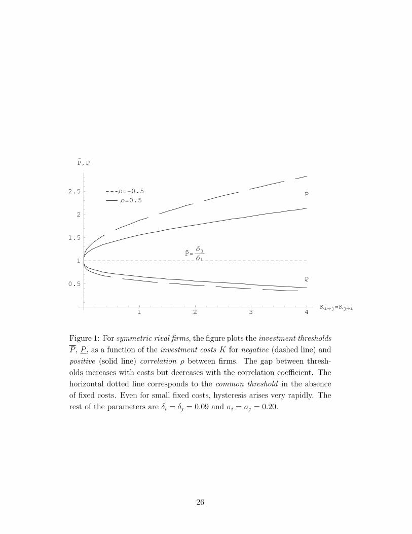
Figure 2 plots the exercise thresholds as a function of volatility for sym-
metric rival firms (δi = δj, σi = σj, Kj→i = Ki→j). The more volatile the
profitabilities of competing firms, the higher the distance between the optimal
exercise thresholds(P, P
). The correlation of changes in rival’s profitabilities
also has an effect which is also apparent in figure 2. P (P ) is monotonically
decreasing (increasing) in ρ. For ρ = 1, the relative profitability of rivals P
is deterministic (ν = 0) and the active firm in the market will be determined
by the initial “yield” criterion in (18) for all time (see also figure 3).
4.2 Calculating the probability of being the active rival
Once one of the two competing firms becomes active in our model, it knows
that it will operate the market only until its rival finds it optimal to claim
the market back. This might well be a finite period of time. What the active
firm would like to know is how long this period of time will be, at least in
expectation. Moreover, for fixed time horizons, what is the probability that
a firm will be active in the market by time t?
To answer these questions, assume that firm j is currently active and the
relative profitability variable is at P0 ∈(P, P
). Define the stopping time Tj
Tj = inf{t ≥ 0 : Pt ≥ P
}
as the first time that P reaches P starting from P0. Since the future evolution
of P is unknown, time Tj is essentially a random variable measuring the time
firm j will be active. Using equation (1.11) in Harrison [9] and an application
of a simple change in variables, the cumulative distribution function of the
first passage time Tj can be written as:
Pr [Tj ≤ t] = Φ
− ln
(PP0
)+ ξt
ν√
t
+
(P
P0
) 2ξ
ν2
Φ
− ln
(PP0
)− ξt
ν√
t
(19)
15
where ξ, ν as in (11) and Φ (.) is the standard normal cumulative distribution
function. To provide a measure of the average time firm j will be active,
one might consider the expected value of Tj. Unfortunately, for the case in
which ξ < 0, the expectation is undefined. Essentially, if the volatility of
the relative profitability measure P is large enough, P may never be reached
and the expectation is infinite, i.e. firm j may remain active for ever. To
overcome this limitation, we choose to measure the average active time of
firm j by the median of Tj. The median active time for firm j, Mj, that
divides the probability in two is the solution to the non–linear equation:
Φ
− ln
(PP0
)+ θMj
ν√
Mj
+
(P
P0
) 2θν2
Φ
− ln
(PP0
)− θMj
ν√
Mj
=
1
2(20)
Figure 4 shows that the median active time of the incumbent firm j increases
with the rival’s investment cost. Notice however the effect of the volatility of
the relative profitability, ν. The median active time Mj decreases with the
volatility of the relative profitability of rivals, ν, i.e. the more volatile the
industry’s profitability, the less the period of time the incumbent firm can
maintain its monopolistic position.
This might seem counterintuitive when viewed in conjecture with the fact
that by definition dνdσi
= dνdσj
> 0, and dPdσi
= dPdσj
< 0 < dPdσi
= dPdσj
, the zone of
hysteresis increases with rivals’ volatilities. The intuition is that an increase
in volatility has a two opposing effects. First, as σi, σj increase, the zone of
hysteresis becomes wider (see figure 2), making it less likely that a change
in the active firm will occur. On the other hand, such an increase makes
the relative profitability process P in (11) more volatile (since ν increases),
increasing the probability that more extreme values of P will be realised
ceteris paribus. It is this second effect that dominates, implying that the more
volatile the market environments, the more short–lived market leadership by
a firm will be.
Once it loses the market to its rival, an incumbent firm would like to
be able to calculate the probability of regaining the market back. In other
words, firm j, if initially active, would like to know what is the probability
that by time T , the relative profitability measure reaches P after having
16
reached P before. Towards that end, define
mPt ≡ max
u∈[0,t]Pu
as the running maximum of the relative profitability process P up to time
t. With P0 ∈(P , P
), we are interested in calculating Pr
[Pt ≤ P ,mP
t ≥ P],
the probability that firm j becomes active again after a finite period of firm
i operating the market. It can be shown that
Pr[Pt ≤ P ,mP
t ≥ P]
= exp
[2θ
ν4ln
(P
P0
)]Φ
ln
(P
P
)− ln(
PP0
)− θt
ν2√
t
(21)
(see for example Musiela and Rutkowski [18, Corollary B.3.1]). Obviously,
this probability increases the further in time we look. For symmetric firms,
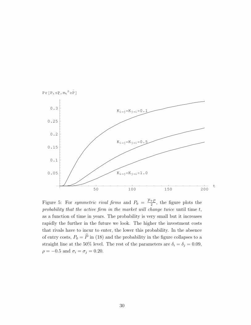
it decreases with the investment entry costs (figure 5) but it increases with
the volatility of firms’ relative profitability ν (figure 6). In figure 5, notice
that as Kj→i = Ki→j → 0, the probability in (21) converges to a straight line
at 50%10, since in this case the thresholds collapse to the unique value P̂ in
(18). Moreover, in figure 6, an increase in ν has again the dual effect discussed
above. The ratio of entry thresholds, γ ≡ P
P, decreases, thus enhancing the
gap between P and P . Moreover, since the volatility of P increases, it is
more probable that more extreme values will be realised. The second effect
dominates to bring the probability in equation (21) up.
5 Aircraft industry application
In this section we apply the model’s main results to an industry that conforms
very closely to our setting: the aircraft manufacturing industry which has
long been dominated by two major competing firms, Boeing Co. and Airbus
Industrie. Stonier and Triantis [25] characterise the industry as a direct
duopoly, report profitability and order volume uncertainty, large irreversible
investments (an average of $5-$10 billion development costs per aircraft type),
10This is true because the initial value of the relative profitability variable is set atP0 = P+P
2 as in all figures.
17
highly differentiated product lines and intense competition where strategic
issues are of great importance.11
On June 23, 2000, the Airbus Industrie’s supervisory board authorised
the launching of the A3XX project, which has been under consideration since
1990. This $13-billion project ($6.125 billion in present value terms, see table
1) entails the construction of the biggest passenger carrier aircraft (550 to
990 passengers), which should guarantee market leadership for the Airbus
consortium in the Very Large Aircraft (hereafter VLA) market segment.12
For the last 30 years, the VLA market had been dominated by the flagship
of the Boeing fleet, the 747-400, until 2000 when Airbus made an enormous
irreversible investment in order to capture the market.
The economics of the A3XX project have been extensively reported and
reviewed by the popular press in the last 3 years (Kane and Esty [11] report a
long list of articles, analysts’ reports and anecdotal evidence concerning the
characteristics and the main uncertainties of the project). However, what
has been an issue of increased speculation, is what would be the possible
reactions of Boeing Co. in the fear of losing its monopolistic position in the
VLA market.
Two likely responses have received much attention in the industry: one
is for Boeing to develop a stretched, 520–seat version of the 747 (the 747X).
The second is to commit to the construction of its own super jumbo jet to
compete head on with the A3XX. In what follows we simulate the model
numerically in an effort to assess the two alternatives.
We estimate the model inputs using the monthly returns of the two com-
panies, from July 2000 (the announcement of the A3XX project) until Jan-
uary 2002. Market data are drawn from Datastream, while some estimates
from Kane and Esty [11] are also used. We estimate Airbus’ equity volatility
at σj = 0.16 and its systematic risk at βj = 0.84, which implies a required
rate of return of approximately µj = 11%.13 The correlation of returns of
11For more on the aircraft manufacturing industry, see the excellent case study by Kaneand Esty [11]. Interested readers can also refer to Hallerstrom and Melgaard [8], Jordan[10] and Stonier [24].
12The VLA market refers to aircrafts with the capacity of seating more than 400 pas-sengers or carrying more than 80 tons of freight.
13The risk–fre rate and the risk premium are assumed at 6%.
18
the two firms is ρ = 0.34 in our sample period.
For Boeing, we use two set of input parameters, representing the two
alternative strategic actions. In the “safer” alternative, the stretch version
of the 747, the investment cost will be substantially lower. Analysts estimate
it at $4 billion (see Dresdner Kleinwort Benson Research report [?]). Since
this alternative will not increase the riskiness of the firm substantially, we
use the historically estimated β = 0.98 for Boeing, which implies µi = 11.9%.
The volatility of Boeing’s returns is σi = 0.15 in our sample. For the “risky”
alternative of building a super jumbo, we use a volatility of 0.30 and a
required return of 13% (an implied beta of 1.17). We do not see any reason
why the investment cost of this alternative should be different from that of
Airbus thus the same investment cost is used. Table 2 summarises the inputs
of our numerical example.
Using the inputs of table 2, the optimal thresholds for Boeing entry in
the VLA are P = 1.78 and P = 2.61 for the “stretch” and “super jumbo”
alternatives respectively. Boeing’s expected operating profitability in the
VLA market should exceed more than twice that of Airbus, for the building
of a corresponding super jumbo to be optimal. This seems very unlikely
even under the most optimistic scenarios concerning the demand in the VLA
market. Since it takes a substantial period of time to construct such an
aircraft14, and with Airbus already locking in key customers with delivery
orders, Boeing can at best expect to share the market with Airbus if a similar
super jumbo is launched.
To further assess the relative attractiveness of the two alternatives, we
estimate the probability that Airbus will maintain leadership of the VLA
market segment under the two proposed reactions of Boeing using equation
(19). Figure 7 shows that the “stretch” alternative decreases the probability
of Airbus’ leadership sharply. Both rivals have a 50% probability of being the
market leader after T = 11.18 years under this alternative. This increases to
T = 18.76 years under the more risky alternative of building a super jumbo
jet.
The above seem to imply that among the two mutually–exclusive alter-
natives considered, Boeing might be better off waiting to build the 520–seat
14Delivery of the first A3XX from Airbus is expected to be in 2006.
19
version of 747 instead of waiting for the riskier super jumbo. Of course the
input parameters used in our model could be questioned. Moreover, some
of the assumptions in the model might seem inappropriate. For example,
Stonier [24] reports that profitability in the aircraft manufacturing industry
exhibits cyclicality, in sheer contrast with our assumption in (1). However,
if the focus is on empirical applications, the discussion above can highlight
that, at a minimum, the model’s intuition could carry over to real business
industries, probably at the expense of analytic tractability.
6 Conclusions
When firms are directly competing for the same market but can exert differ-
ent and uncertain future profits from operations, investment timing becomes
a strategic decision variable which can be optimised conjecturing the rival’s
optimal response. We solve a stochastic real option game under the assump-
tion that only one firm can be active at any point in time, but its idle rival
has the option to reclaim the market whenever optimal to do so. This is only
possible because the homogeneity of the problem in the two state variables
allows reduction of its dimensionality to one.
In the absence of fixed entry costs, optimal entry strategies are shown
to conform to a simple criterion: invest if your opportunity cost of remain-
ing idle exceeds your rival’s operating yield, i.e. the firm with the highest
current yield (opportunity cost) operates the market. When fixed costs are
introduced, the optimal rival investment thresholds are shown to be sepa-
rated in the two state variable space, producing a hysteresis range, and the
active firm in the market is history–dependent. Optimal entry strategies are
then determined by a simple, easily invertable, non–linear equation which
uniquely describes the hysteresis system.
The range of hysteresis in entry thresholds is increasing in the investment
costs but decreasing in the correlation between rivals. The effect of volatility
however is dual : on one hand, volatility widens the gap of hysteresis driving
the optimal entry times of rivals further apart. On the other hand though,
the higher the volatility, the more probable big changes in the firms’ prof-
itabilities will be realised in a shorter period of time. It is this second effect
20
that dominates, thus making more volatile markets proner to more fierce
competition and more changes in market leadership.
21
A Appendix
A.1 Derivation of ODE in (5)
Successive differentiation of (4) yields
∂Fj→i(Si, Sj)
∂Si
= f ′j→i(P )
∂Fj→i(Si, Sj)
∂Sj
= fj→i(P )− Pf ′j→i(P )
∂2Fj→i(Si, Sj)
∂S2i
=1
Sj
f ′′j→i(P )
∂2Fj→i(Si, Sj)
∂S2j
=1
Sj
P 2f ′′j→i(P )
∂2Fj→i(Si, Sj)
∂Si∂Sj
= − 1
Sj
Pf ′′j→i(P )
Substituting the above in equation (2) and simplifying yields
1
2
[σ2
i S2i
1
Sj
− 2ρσiσjSiSj1
Sj
P + σ2j S
2j
1
Sj
P 2
]f ′′j→i(P ) + (r − δi) Sif
′j→i(P )
+(r − δj)Sj
(fj→i(P )− Pf ′j→i(P )
)− rSjfj→i(P ) + Sj = 0
Divide through with Sj and collect terms to get equation (5) in the text.
22
References
[1] F. M. Baldursson. Irreversible investment under uncertainty in oligopoly.
Journal of Economic Dynamics and Control, 22(4):627–644, 1998.
[2] M. J. Brennan and E. S. Schwartz. Evaluating natural resource invest-
ments. Journal of Business, 58(2):135–157, 1985.
[3] A. K. Dixit. Entry and exit decisions under uncertainty. Journal of
Political Economy, 97(3):620–638, 1989.
[4] A. K. Dixit and R. S. Pindyck. Investment under Uncertainty. Princeton
University Press, New Jersey, 1994.
[5] B. Dumas. Super contact and related optimality conditions. Journal of
Economic Dynamics and Control, 15(4):675–685, 1991.
[6] B. Dumas and E. Luciano. An exact solution to a dynamic portfolio
choice problem under transaction costs. Journal of Finance, 46(2):577–
595, 1991.
[7] S. R. Grenadier. The strategic exercise of options: Development cas-
cades and overbuilding in Real Estate markets. Journal of Finance,
51(5):1653–1679, 1997.
[8] N. Hallerstrom and J. Melgaard. Going round in cycles. Airfinance
Journal, 239(March):49–52, 1998.
[9] M. J. Harrison. Brownian Motion and Stochastic Flow Systems. Robert
E. Krieger Publishing Company, 1985.
[10] W. S. Jordan. New aircraft orders: Still a leading indicator of airline