63
STREAM FLOW Guest Lecture By: M. Tugrul Yilmaz [email protected] Hydrosphere (EOS 656) April 06, 2010 Image courtesy of National Geographic
| Date post: | 18-Aug-2018 |
| Category: |
Documents |
| Upload: | trinhtuyen |
| View: | 213 times |
| Download: | 0 times |

STREAM FLOW
Guest Lecture
By: M. Tugrul [email protected]
Hydrosphere (EOS 656)
April 06, 2010
Image courtesy of National Geographic

2Image courtesy of USGS, http://ga.water.usgs.gov/edu/watercycle.html
Stream flow is a body of water that is flowing on Earth’s surface.
It is, arguably, the most important component of hydrological cycle that effects us directly (socially, economically, politically).
3
economically, politically).
It is a major source for our drinking water and agricultural needs, a habitat for living organisms, a source for electricity production, and sometimes the disaster itself.

4
Streamflow is a residual of the other water cycle elements; hence its accurate indirect estimation (through other parameters) is still a challenge.
Image courtesy of MIT, ocw.mit.edu/OcwWeb/Civil-and-Environmental-Engineering/1-72Fall-2005/LectureNotes/

1- Basic TermsRiparian Zones are the ecosystems at the interface between land and rivers.
Watershed is a piece of land that all the water that falls on the ground drains into a river.
Tributaries are small streams or rivers that flow into larger rivers.
5
rivers that flow into larger rivers.
Image courtesy of www.anra.gov.au/topics/vegeta tion/pubs/biodiversity/bio_assess_conservation.html
Image courtesy of http://techalive.mtu.edu/meec /module01/Watershed.html

Infiltration Rate: The capacity of soil to suck the available water at the surface (or at lower layers). It is inversely related with the saturation of soil.
Overland Flow: Can happen in two ways:
1) When the rainfall intensity exceed the infiltration rate of
Hortonian Overland Flow
6
exceed the infiltration rate of soil (also called HortonianOverland Flow).
2) When the groundwater table rises up to the surface (also called Saturation Overland Flow).
Image courtesy of http://www.flickr.com/photos/15157983@N00/211869881

Gaining Stream
Loosing Stream
7
Dry Stream Bed
Image courtesy of http://www.salemstate.edu/
~lhanson/gls100/gls100_hydro.htm

How is Streamflow born?
8
Image courtesy of MIT, ocw.mit.edu/OcwWeb/Civil-and-Environmental-Engineering/1-72Fall-2005/LectureNotes/

2- Measuring/estimating Stream flow
9

Measuring Discharge
Weirs are structures that have known area – discharge relationship (depending on some other empirical parameters).
Advantage: Water head is the only necessary measurement needed to estimate the discharge.
10
Q = C*L*HQ is the discharge (flow rate over the weir)C is the effective coefficient of dischargeL is the length of the weir crestH is the head measured above the weir crest

V-notch
weir
Rectangular
weir
11
Image courtesy of http://www.lmnoeng.com/Weirs/RectangularWeir.htm
Cipoletti
weir
Other types include triangular and circular. Among them rectangular weir is the most
common type whereas V-notch type gives more sensitivity to the discharge.

12
Image courtesy of http://tiee.ecoed.net/vol/v1/data_sets/hubbard/fig1stream.jpg

13

Estimating Discharge, Q = V *A
14
Q = V * AQ=discharge (m3/sec) V=Velocity(m/sec)A=Area(m2)
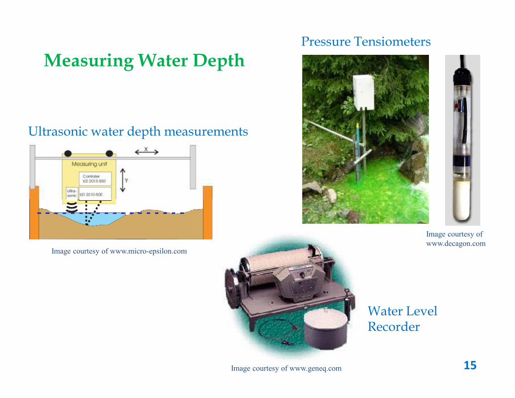
Measuring Water DepthPressure Tensiometers
Ultrasonic water depth measurements
15
Image courtesy of www.micro-epsilon.com
Image courtesy of www.geneq.com
Water Level Recorder
Image courtesy of
www.decagon.com

Rating curves
16
Image courtesy of http://www.utdallas.edu/~brikowi/Teaching/Field_Methods/sanders-1998_fig3-22.jpg

Q = V * A
Velocity profile along the river (both horizontally and vertically) is not uniform!!!
Measuring Velocity
17
vertically) is not uniform!!!
An average value is needed. Two options:
1) Measure the velocity of the river both horizontally and vertically for predetermined locations (and take an average value).
2) Using open channel (Manning Equations)
Image courtesy of USGS, http://ga.water.usgs.gov/edu/streamflow2.html

Stream width
0ft0ft0ft0ft 10ft10ft10ft10ft
1ft 1ft 1ft 1ft .... 9ft9ft9ft9ft3ft3ft3ft3ft . . . . 5ft5ft5ft5ft . . . . 7ft 7ft 7ft 7ft . . . . River bank
River bank
Place where a measurement is made
Water level
1ft1ft1ft1ft
Stream depth
Place where a measurement is made
2ft2ft2ft2ft
3ft3ft3ft3ft
Q = A* Vw
Q = discharge (ft3/sec)A = surface are (ft2)Vwwater velocity (ft/sec)Qtotal = Q1 + Q2 ….Qn
19
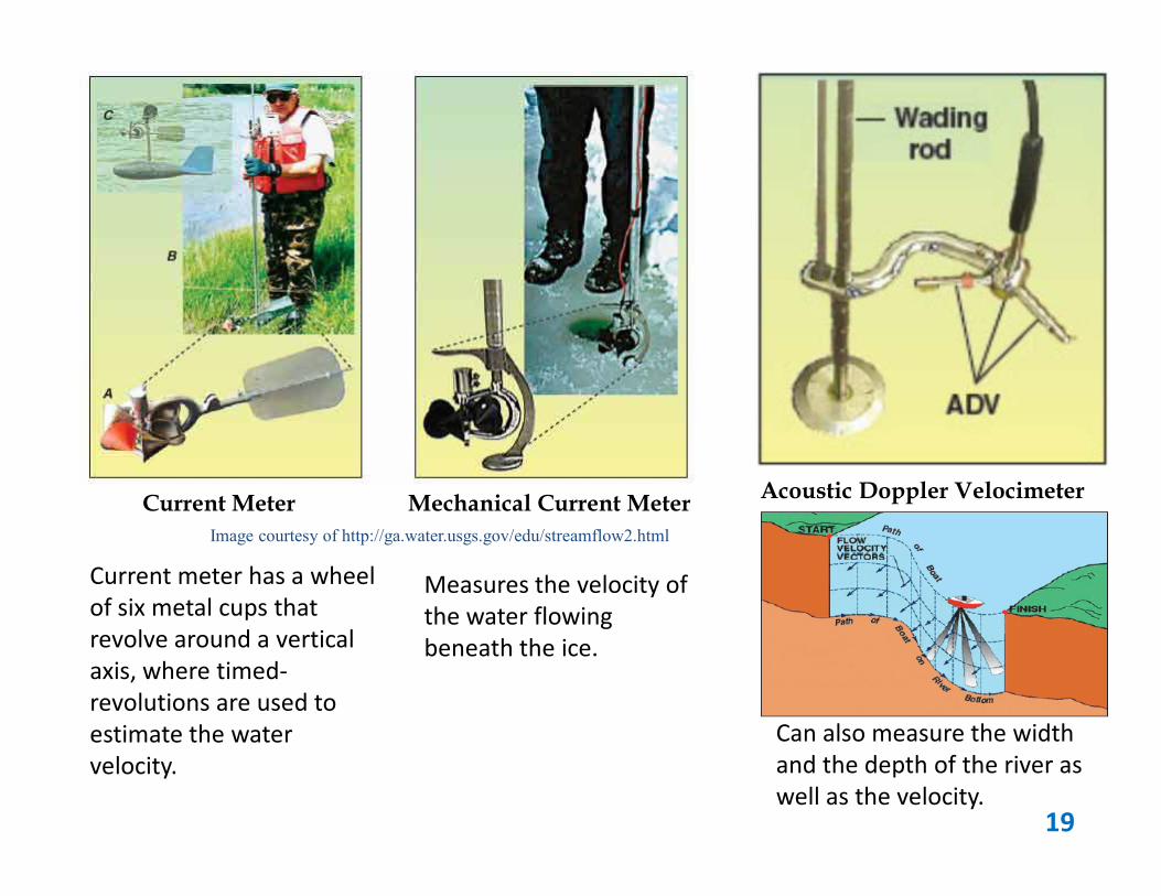
Acoustic Doppler VelocimeterCurrent Meter Mechanical Current Meter
Current meter has a wheel
of six metal cups that
revolve around a vertical
axis, where timed-
revolutions are used to
estimate the water
velocity.
Image courtesy of http://ga.water.usgs.gov/edu/streamflow2.html
Measures the velocity of
the water flowing
beneath the ice.
Can also measure the width
and the depth of the river as
well as the velocity.

More primitive ways:
Branch Method: Throw a branch of tree at the up stream and
measure the travel time it takes for a particular distance.
Salt Method: Prepare a bucket of salty water (very dense). Then, dump the bucket in the river and continually measure the
20
dump the bucket in the river and continually measure the conductivity (EC) of the river. From the EC change in time, the speed of the river can be estimated.
But these methods only give the speed of the water at the points where the measurements are done; but wouldn’t provide a profile info.

Estimating Velocity using Manning Equations
21
R, ratio of cross-sectional area to wetted perimeter of channelS, is slope of water surfaceN, is the Manning channel roughness coefficient
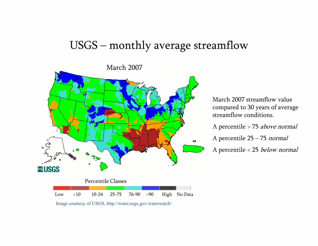
USGS – monthly average streamflow
March 2007
March 2007 streamflow value compared to 30 years of average streamflow conditions.
A percentile > 75 above normal
Image courtesy of USGS, http://water.usgs.gov/waterwatch/
A percentile > 75 above normal
A percentile 25 – 75 normal
A percentile < 25 below normal
Low <10 10-24 25-75 76-90 >90 High No Data
Percentile Classes

How about recovery of historical Streamflow??
23
In this study, trees (at slopes located at higher altitudes than rivers) were assumed to have
strong relation between its growth and the overall water balance (related to streamflow) of
its watershed. Hence, the tree rings were used to extract historical streamflow info.
Image Courtesy of http://wwa.colorado.edu/treeflow/lees/treering.html

3- Precipitation - Discharge relation
Depending on soil characteristics, soil moisture, and the nature of the storm, each watershed have a different precipitation – discharge response.
Hyetographs (Precipitation change in time)(Unit) Hydrographs (Discharge change in time under a constant precipitation rate)
Initial Abstraction Initial soil absorption of precipitation (no discharge)
24
Initial Abstraction Initial soil absorption of precipitation (no discharge)Rising Limb Increase in discharge due to intensified stormFalling Limb Decrease in discharge due to recessing stormPeak Discharge Maximum amount of discharge that the storm producesLag Time The time delay between the time of peak discharge and the precipitationRunoff Overland flow that feeds the streamThrough flow Horizontal sub-surface movement of water. It first appears at the surface before it merges to stream, lake, etc.Inter flow (Sub-Surface flow) Same as through flow; but it does not appear at surface before merging.Baseflow Groundwater flow that discharges to stream.

Image courtesy of S. L. Dingman, Physical Hydrology,
Drainage Area effect
25

Total Hydrograph vs Unit Hydrograph
400
500
600
700
800
900
1000
Discharge
Unit Hydrograph and Total Hydrographs
10 inch event
4 inch event
1inch event (unit Hydrograph)
Unit hydrograph is the response of the drainage area to a unit (1 inch/ 1mm) volume of runoff.
0
100
200
300
400
0 1 2 3 4 5 6 7 8 9 10 11 12 13 14
Discharge
Time
Unit hydrographs are estimated from historical data.Any amount of excess runoff can be calculated from unit hydrographs
26
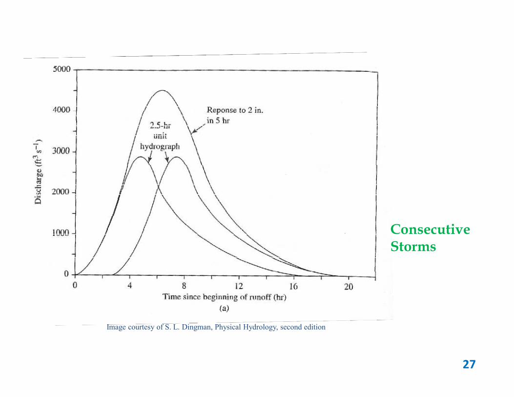
Image courtesy of S. L. Dingman, Physical Hydrology, second edition
Consecutive Storms
27

Rainfall-Discharge relation in space and time
The influence of rainfall spatial distribution
Catchment representation
The influence of rainfall intensityThe influence of rainfall duration
Image courtesy of http://hydram.epfl.ch/VICAIRE/ 28
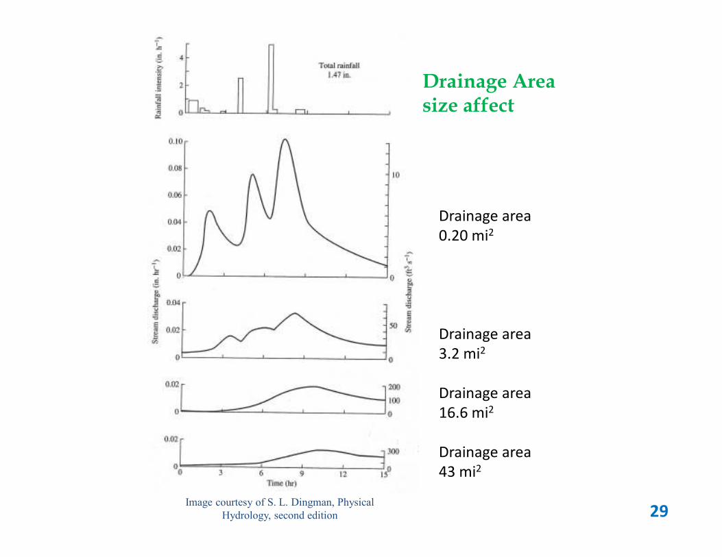
Drainage Area size affect
Drainage area
0.20 mi2
Image courtesy of S. L. Dingman, Physical
Hydrology, second edition
Drainage area
3.2 mi2
Drainage area
16.6 mi2
Drainage area
43 mi2
29

Hydrological response to precipitation type
1.5
2
2.5
3
Str
ea
m f
low
Snow Dominated
Rain and Snow
Rain Dominated
0
0.5
1
1.5
0 1 2 3 4 5 6 7 8 9 10 11 12
Str
ea
m f
low
Month
10 11 12 1 2 3 4 5 6 7 8 9
30

Rainfall – Runoff relation of a storm event
Hyetograph
Hydrograph
Total rainfall Net rain Hydrograph
Transformation of total rain in Hydrograph
Image courtesy of http://hydram.epfl.ch/VICAIRE/
Loss due to
evaporation, soil
storage, etc
Effective Water
Input
31
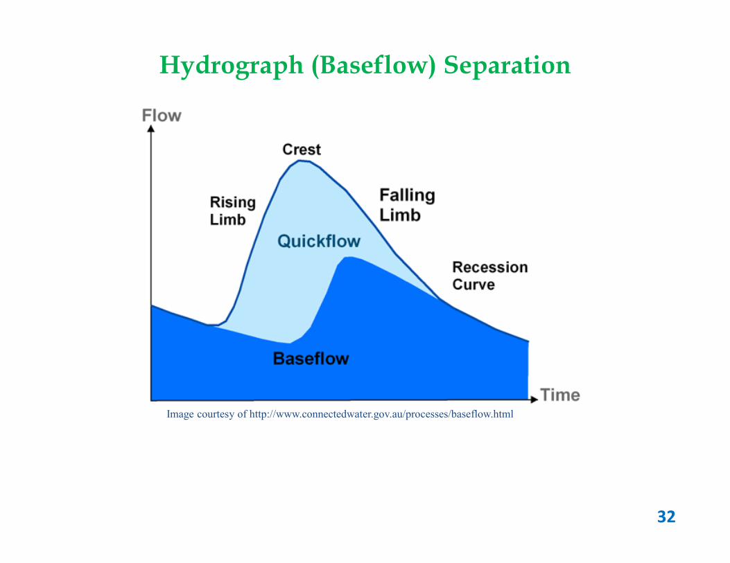
Hydrograph (Baseflow) Separation
32
Image courtesy of http://www.connectedwater.gov.au/processes/baseflow.html

a) Graphical Separation Methods
Constant-discharge method: Baseflow is assumed constant at the (minimum) discharge level before rising limb starts.
Constant-slope method: Falling Limb inflection point is connected to the beginning of rising limb. For large watersheds, the inflection point is estimated by empirical formulas.
Concave method: Extend the hydrograph right before the rising limb until the time of peak discharge. Then connect that point to the inflection point of
33
the time of peak discharge. Then connect that point to the inflection point of the falling limb. This method assumes the baseflow decreases during the rising limb and increases during falling limb.
Master Depletion Curve method: Several depletion curves are used to obtain an average slope of the falling limb.
0
2
4
6
8
10
12
14
16
1
Discharge (m3/s)
Time (hours)
Constant-
Slope
Concave
Method
Constant-
discharge

Master Depletion Curve
34
Figure Courtesy of T. Brikowski www.utdallas.edu/~brikowi/Teaching/Applied_Modeling
b) Time Series Processing Methods
These methods may not have hydrological basis. They use the time series of discharge data to obtain useful baseflow information.
The baseflow index (BFI): Long-term ratio of baseflow to total streamflow
35
Mean annual baseflow volume
Long-term average daily baseflow
Filtering the discharge time series: (i.e. filtering the high frequency runoff to obtain baseflow)

c) Isotope Separation Methods
Water molecule is formed by O-2 and H+ elements. 16O is the most common oxygen isotope
•Heaviest isotopes of the perceptible water fall first. Then lighter isotopes.
•Lightest isotopes evaporates first. Then heavier isotopes.
Using Isotope dating methods to estimate the origin and the age of the water to separate the baseflow and the overland flow.
36
Then heavier isotopes.
18O / 16O ratio of human scalp hair.
Image courtesy of Ehleringer J R et al. PNAS 2008;105:2788-2793
overland flow.

4- Rainfall Runoff Models
For long term averages, rainfall and the basin area information can be used to model the amount of runoff that a particular storm would produce.
200
250
300
350
400
Dis
cha
rge
(m
m)
37
Models are needed to estimate the peak of the discharge and prediction of floods.Two examples of these models are Rational method and the SCS method.
0
50
100
150
200
100 200 300 400 500 600 700 1000
Dis
cha
rge
(m
m)
Precipitation (mm)

The Rational Method
Qmax = C * I * A
Qmax : Is the peak discharge (m3/day)
C : Constant (dependent on soil/cover)
I : Intensity of the rain (mm/day)
A : Area of the watershed (m2)
38
A : Area of the watershed (m2)
More accurate for smaller watersheds!! (~ <50 acres=400m*500m)
Downtown
Crop/Agriculture
C= 0.70 – 0.95
C= 0.05 – 0.25

SCS Curve number Method
Based on the antecedent soil wetness
conditions and the soil type, this
method relates the effective water
input (Weff) to the amount of rainfall.
1) Obtain Curve number for the
watershed based on the land cover and
conditions.
2) Adjust CN for watershed wetness
39
Image courtesy of S. L. Dingman, Physical
Hydrology, second edition
2) Adjust CN for watershed wetness
3) Calculate Vmax
4) Calculate Weff
Vmax=1000/CN – 10
Weff = (W – 0.2* Vmax)2 / (W + 0.8* Vmax)
Vi =0.2 * Vmax (for normal wetness)
Vi : Initial AbstractionVr : RetentionQeff : Event FlowW : Hyetograph of water inputVmax: Maximum Retention capacity
TOPMODEL bases its distributions on the topography of the drainage basin.
How about topography?
40
The model estimates the saturation excess and infiltration excess (Hortonian) surface runoff and subsurface flow.

Flash Flooding occurs minutes or hours of a heavy rainfall event which causes water levels to rise rapidly.
River Flooding happens as a result of the heavy rains related with
Flood Types:
5- Floods
41
River Flooding happens as a result of the heavy rains related with decaying storms.
Seasonal watershed characteristics:
Spring: Snow melt, moist soil � Higher level streamflowSummer: High evaporation, drier soil � Lower level flows.

January 2000 February 2000 March 2000
USGS Historic Maps of Monthly and Annual Streamflow
Image courtesy of USGS http://water.usgs.gov/nwc/
April 2000 May 2000 June 2000
Above normal Normal Below normal
42

The final 2007-2008 seasonal snowfall map of Wisconsin, record setting for parts of Southern Wisconsin. For example, Madison WI received 101.4 inches surpassing the
Example of heavy snow melt
Image courtesy of http://commons.wikimedia.org/wiki/File:2007
-08_Winter_Snowfall_in_Wisconsin.png
inches surpassing the previous record of 76.1 inches.
43

Dodge County, WI, June 14, 2008 -- Farms and homes are under water flooding in the rural areas of Wisconsin continues. Barry Bahler/FEMA Image courtesy of http://commons.wikimedia.org/wiki/Category:Wisconsin_flood_of_2008
44
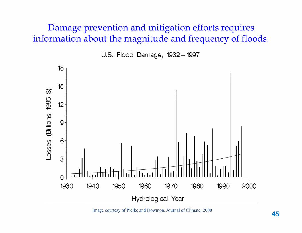
Damage prevention and mitigation efforts requires information about the magnitude and frequency of floods.
45Image courtesy of Pielke and Downton. Journal of Climate, 2000

Probability of FloodsIn general peak (max) discharge in a given year is the parameter of interest for flood design studies.
Probability : Likelihood of a discharge to happen in any given year
Return Period : On average, how many years is any given event would repeat.
EXAMPLE-1: Given we have 100 years of streamflow data. To
46
EXAMPLE-1: Given we have 100 years of streamflow data. To calculate the probability of a given discharge:
- Rank the available discharge data - Find the corresponding rank of the discharge to be investigated- P = rank / #observations - T= 1 / P
WARNING!!! Do NOT attempt to calculate any probability exceeding the historically available maximum discharge.

EXAMPLE-2: What is the probability that an event with a discharge of Q will happen at least once in the next 15 years?
-Find the probability that corresponds to Q (assume p1)-Pat least once = 1 – Pnone= 1 – (1 - p1)
15
Occurrence of a storm does not affect the chances that the storm would happen next (or in the same) year again!!
47
EXAMPLE-3: The return year (T) of a storm with 200 years return periodP=1/200=0.005
Chances that two storms with the same magnitude would happen (same year)P=0.005*0.005 = 0.000025

Katrina: Based on the 100 years of historical data (includes Hurricane Ethel in 1960, 71 m s-1; Hurricane Carla in 1961, 77 m s-1; Hurricane Camille in 1969, 85 m s-1), Elsner et al. (2006, G.R.L., 33, L08704) builda model. Model has
5-year return level of 54 m s-1
50-year return level of 77 m s-1
500-year return level of 88 m s-1
According to this model, Hurricane Katrina (with maximum wind
48
According to this model, Hurricane Katrina (with maximum wind speed of 71 m s-1) has return period of 21 years with 95% confidence levels at 10-50 years.
When model was extended to include the entire U.S. coast from Texas to Maine, a return period of 14 years was found for hurricanes with wind speed equal to Katrina with a 95% interval range from 9 to 30 years.

High and Low streamflow conditions
Map of flood and high flow conditions for April 5, 2010
Map of below normal 7-day average streamflow compared to historic streamflow for April 4, 2010
Image courtesy of http://waterwatch.usgs.gov/?m=flood,map&r=us&w=real,map
Percentile classes
95-98 >=99 above flood average
Percentile classes
Low <=5 6-9 10-24 insufficient data
49

Remote Sensing and GIS provides the excellent sources and tools to assess, manage, and identify the impact of floods.
MODIS images of Monsoon Flooding in India, Image courtesy of http://visibleearth.nasa.gov/view_rec.php?id=20072
Image courtesy of www.esri.com/industries/water_resources/Image courtesy of http://www.crh.noaa.gov/images/
50

6-) Effect of climate change
Image courtesy of http://global-warming.accuweather.com/blogpics/map_blended_mntp_02_2007_pg.gif 51

http://global-warming.accuweather.com/blogpics/map_blended_mntp_02_2007_pg.gif
52

LOW FLOW: The Colorado River is one of several around the world losing water. Image courtesy of ZUMA Press http://www.mnn.com/earth-matters/climate-change
53

Annual streamflows into Perth’s dams
Figure courtesy of http://www.garnautreview.org.au/chp5.htm
54

Precipitation Anomalies
Image courtesy of http://www.prism.oregonstate.edu/index.phtml 55

ImpactsImpacts RegionRegion
Coastal flooding/erosion South, Southeast, Mid-Atlantic, Northeast, Northwest, Alaska
Hurricanes Atlantic and Gulf of Mexico coastal areas
Decreased snow cover and ice, more intense winter storms
Alaska, West, Great Lakes, Northeast
Flooding/intense precipitation All regions, increasing with higher northern
Projected U.S. Regional Climate ImpactsProjected U.S. Regional Climate Impacts
Flooding/intense precipitation All regions, increasing with higher northern latitude
Sea-level rise Atlantic and Gulf of Mexico coastal areas, San Francisco Bay/Sacramento Delta region, Puget Sound, Alaska, Guam, Puerto Rico
Decreased precipitation and stream-flow Southwest
Drought Portions of the Southeast and Southwest
Wildfires West, Alaska
Intense heat waves All regions
Courtesy of http://www.pewclimate.org/docUploads/
56

Change in runoff based on streamflow data
Image courtesy of http://www.laboratoryequipment.com/news-climate-change-river-level-drops-042209.aspxTime period: 1948-2004
57

Annual runoff projection by four climate models
Image courtesy of http://www.theclimatechangeclearinghouse.org/HydrologicEffects/ChangesAnnualAvgRunoff/default.aspx
Percentage changes in average annual runoff projected by four climate models for the period 2090-2099, relative to 1980-1999 Source: IPCC. 2007. Climate Change 2007: Synthesis Report. Intergovernmental Panel on Climate Change. Figure 3.5, p. 49.
58

More room for climate change studies than ever!
Climate change impact on:
- Freshwater systems
(availability, sustainability)
- Human Health
- Ecosystems
- Existing Infrastructure
59
- Existing Infrastructure
- Financial cost
- …
For future:
- Adaptation & Mitigation studies
- Risk/Vulnerability analysis

USGSUSGSUSGSUSGS Daily Streamflow Conditions Real-Time Water Data for the Nation
Appendix-1 - Where to get the data?
USGSUSGSUSGSUSGS observation stationSite name: San Lorenzo CreekLocation: near King city, CADrainage area: 233 miles2
Period of recorded data: Oct 1958 to currentGage datum: 431.8 feet ASL NGVD29
High
>90th percentile
75th – 89th percentile
25th – 74th percentile
10th – 24th percentile
< 10th percentile
Low
Not rated
Note: Percentile is computed from the period of record for the current day of year. Only stations with at least 30 years of record are included.
60

USGS DAILY STREAMFLOW DATA DOWNLOAD
-http://nwis.waterdata.usgs.gov/nwis
Surface Water
61
Daily Data
Site Name/Location/etc.
SUBMIT

Appendix-2 – Related LinksUSGS
http://waterwatch.usgs.gov/
http://water.usgs.gov/osw/
http://nwis.waterdata.usgs.gov/nwis
EPA
http://www.epa.gov/watertrain/
NOAA
http://www.katrina.noaa.gov/helicopter/helicopter-2.html
62
http://www.katrina.noaa.gov/helicopter/helicopter-2.html
http://www.nhc.noaa.gov/HAW2/english/storm_surge.shtml
IPCC
http://www.ipcc.ch/publications_and_data/publications_and_data_reports.htm
FEMA
http://www.fema.gov/hazard/flood/index.shtm
UCAR
http://www.ucar.edu/communications/factsheets/Flooding.html
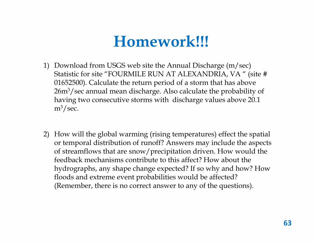
Homework!!!
1) Download from USGS web site the Annual Discharge (m/sec) Statistic for site “FOURMILE RUN AT ALEXANDRIA, VA “ (site # 01652500). Calculate the return period of a storm that has above 26m3/sec annual mean discharge. Also calculate the probability of having two consecutive storms with discharge values above 20.1 m3/sec.
63
2) How will the global warming (rising temperatures) effect the spatial or temporal distribution of runoff? Answers may include the aspects of streamflows that are snow/precipitation driven. How would the feedback mechanisms contribute to this affect? How about the hydrographs, any shape change expected? If so why and how? How floods and extreme event probabilities would be affected? (Remember, there is no correct answer to any of the questions).


