STRUCTURAL INTERACTIONS AND LONG RUN GROWTH AN …

Revue de l’OFCE / Debates and policies – 124 (2012)

STRUCTURAL INTERACTIONS AND LONG RUN GROWTH

AN APPLICATION OF EXPERIMENTAL DESIGN TO AGENT-BASED MODELS1

Tommaso Ciarli SPRU, University of Sussex, UK

We propose an agent-based computational model defining the following dimen-sions of structural change—organisation of production, technology of production,and product on the supply side, and income distribution and consumption patternson the demand side—at the microeconomic level. We define ten different parametersto account for these five dimensions of structural change. Building on existing resultswe use a full factorial experimental design (DOE) to analyse the size and significancethe effect of these parameters on output growth. We identify the aspects of structuralchange that have the strongest impact. We study the direct and indirect effects of thefactors of structural change, and focus on the role of the interactions among the diffe-rent factors and different aspects of structural change. We find that some aspects ofstructural change—income distribution, changes to production technology and theemergence of new sectors—play a major role on output growth, while others—consumption shares, preferences, and the quality of goods—play a rather minor role.Second, these major factors can radically modify the growth of an economy evenwhen all other aspects experience no structural change. Third, different aspects ofstructural change strongly interact: the effect of a factor that influences a particularaspect of structural change varies radically for different degrees of structural changein other aspects. These results on the different aspects of structural change provide anumber of insights on why regions starting from a similar level of output and withinitial small differences grow so differently through time.

Keywords: Structural change, Long run growth, ABM; DOE.

1. The paper builds on previous work and discussions with André Lorentz, Maria Savona andMarco Valente, to whom I am indebted for their advice, suggestions, and support. Insightfulcomments from a referee helped to improve significantly the paper. This work is based on anintensive use of simulations that would have not been possible (or would have taken a fewyears) without the access to the computer cluster of the Max-Planck-Institut für Mathematik inden Naturwissenschaften in Leipzig, facilitated by Rainer Kleinrensing, Ronald Kriemann, andThomas Baumann. Financial support by the Max Planck Institute of Economics in Jena, where Ihave conducted a substantial part of the present research as a research fellow in theEvolutionary Economics group, is gratefully acknowledged. Any error is my own responsibility.

Tommaso Ciarli296

The dramatic increase in output and consumption followingthe industrial revolution was accompanied by substantial changesin the structure of the economies involved. Countries of late indus-trialisation and current transition countries are also experiencingdramatic changes (Dasgupta and Singh, 2005). Economists usuallyrefer to structural change as the reshuffling in the share of employ-ment or value added in the three main sectors: agriculture,manufacturing and services (Clark, 1940; Fisher, 1939; Dietrich andKrüger, 2010; Baumol, 2010) which has led to these grandeconomic shifts to be described as ''industrialisation'' and''tertiarisation'' of advanced economies. However, structuralchanges encompass more than shifts in labour and value addedfrom one sector to another; they include complex adjustments inthe structure of production, consumption, labour organisation andincome distribution, which interact in a continuous evolutionaryprocess. For instance, industrialisation is accompanied by theconcentration of production in large capital intensive firms andfirm size growth (Desmet and Parente, 2009), an increase in thenumber of goods available for final consumption (Berg, 2002),closer involvement of science in technological change (Mokyr,2002), increased use of capital in agriculture and especially manu-facturing accompanied by an improvement in the technologyembedded in new machines and overall increases in productivity(Kuznets, 1973), greater urbanisation usually accompanied byincreased income inequality and changes in social class composi-tion (McCloskey, 2009), and so on. In other words, industrialisationleads to transformations of economies and societies. Thus the defi-nition proposed by Matsuyama, that structural change is''complementary changes in various aspects of the economy, suchas the sector compositions of output and employment, the organi-sation of industry, the financial system, income and wealthdistribution, demography, political institutions, and even thesociety's value system'' (Matsuyama, 2008).

To be sure, some changes precede income growth, others unfoldas a consequence of income growth, and there are interactionsamong the different aspects of structural change. For instance,changes in the distribution of income are related to changes inclass composition and patterns of consumption. Changes to class

Structural interactions and long run growth 297

composition, in their turn, are related to the accumulation ofcapital and the different organisation of labour. The accumulationof capital induces the search of new technologies embedded inmore efficient capital goods, and so on.

Ideally we would like to explain the changes in each aspect ofstructural change, their co-evolution and their effect on the direc-tion of economic growth and on other dimensions of structuralchange. We believe that such an investigation is fundamental toshed light on the determinants and dynamics of long-run growth,and to derive policy implication that consider different aspect ofeconomic change. This is especially relevant since traditionalexplanations of the relation between structural change and growthpoint to opposing dynamics (Matsuyama, 2008): i) exogenouschanges in productivity in the manufacturing sector—whichsomehow emerge in the economy—induce labour migration fromagriculture to industry; and ii) an increase of productivity in agri-culture reduces demand for labour and induces migration to themanufacturing sector where capital investment—characterised byhigher increases in productivity per unit of investment—spursgrowth; the more investment that is concentrated in manufactu-ring, the greater manufacturing productivity increases. Both thesemechanisms are plausible. However, taken in their basic versionthey do not acknowledge the wide array of ''complementarychanges'' they are conducive to, and which help in solving theircontradiction. We believe that a more accurate explanation shouldinclude the various economic aspects that accompany the transfor-mation of an economy.

In this paper we heed Matsuyama (2008) definition of structuralchange and model complementary changes in various aspects ofthe structure of an economy, namely organisation of production,technology of production, and product on the supply side, andincome distribution and consumption patterns on the demandside. However, we also follow Saviotti and Gaffard (2008) sugges-tion and investigate the microeconomic sources of structuralchanges. Saviotti and Gaffard (2008, p. 115), in line withMatsuyama (2008), define structural change as a ''change in thestructure of the economic system, that is, in its components and intheir interactions. Components are [...] particular goods orservices, and other activities and institutions, such as technologies,

Tommaso Ciarli298

types of knowledge, organisational forms etc.''. However, departingfrom Matsuyama (2008), they ask: ''What does it mean for a systemto be in equilibrium when its composition keeps changing due tothe emergence of qualitatively different entities?'' [p. 116].

We take on board these remarks and propose a model of themicroeconomic dynamics of structural change as processes thatnever reach equilibrium, because of the continuous changes to theunderlying dimensions of the economy. In order to model thesemicroeconomic interactions and study the emergent structuralchange and aggregate output, we use computational models andsolutions (Colander et al., 2008; LeBaron and Tesfatsion, 2008;Dosi et al., 2010; Leijonhufvud, 2006; Buchanan, 2009; Delli Gattiet al., 2010; Dawid and Semmler, 2010).

We propose an agent-based computational model defining thefollowing dimensions of structural change—organisation ofproduction, technology of production, and product on the supplyside, and income distribution and consumption patterns on thedemand side—at the microeconomic level. We model their co-evolution in terms of the interactions among the different agentson the supply and demand sides, and the changing behaviourpromoted by changes to income and structure. We contribute tothe traditional literature on structural change by accounting for'complementary changes' and in a micro to macro framework,which can be treated exhaustively using agent based computa-tional models.

The model includes two types of firms: capital and final goodsproducers. Final goods producers produce goods that satisfy diffe-rent consumption needs, serving different markets. New marketsemerge as an outcome of firms' investments in innovation.Consumer goods differ also with respect to their quality. A firmincludes many layers of employees (workers and managers at diffe-rent levels), with each layer earning a different wage. This createsconsumers with unequal income distribution. Consumers aregrouped into classes that demand different varieties of goods, affec-ting firm demand. Among other things, this implies that the largerthe number of organisational layers required in the firm (organisa-tional complexity), the higher are the differences across consumers,ceteris paribus. Each class distributes its consumption differentlyacross the different markets. These consumption shares evolve


endogenously as new classes emerge in the economy, representingEngel curves. Growth results from demand expansion, which is ajoint outcome of firm selection and technology investment.

The structure of the model is based on Ciarli et al. (2010) andCiarli and Lorentz (2010), which discuss the micro economic dyna-mics that lead to growth in output via endogenous changes indifferent aspects of economic structure. Ciarli et al. (2012) discussthe non-linear effects of organisational complexity, productiontechnology and product variety on income growth and distribu-tion. They show that output is negatively related to initial productand demand variety, organisational complexity and faster techno-logical change in capital goods increase output despite higherinequality, and this last, in the form of large earning disparities,leads to lower output growth.

In this paper we build on existing results and assess the relativeimportance of all the factors that, in the model, determine theinitial conditions of structural change and also the pace at whichthe different aspects of the economic structure evolve. The organi-sation of production is defined by the structure of labour andearnings disparities. Production technology is defined by the speedof change in capital innovation, the share of resources invested inR&D, and its success. Product technology is defined by the abilityof firms to explore new sectors for a given level of R&D invest-ment, improved quality of a new product, and share of resourcesinvested in R&D. Income distribution is studied in relation toprofits in capital and final goods firms. Consumption patterns aredefined by the speed at which consumption shares change withincreases in income and class differentiations and changes inconsumer preferences promoted by the emergence of differentincome classes. Whilst we define each aspect of structural changebased on specific factors, most of these factors induce structuralchange in several aspects of the economy. For instance, the organi-sation of labour has an impact on the evolution of income classesand, therefore, also on patterns of consumption; the resourcesinvested in R&D reduce the profits available to be shared amongfirm managers, which affects income distribution; and so on.

We use a full factorial experimental design (DOE) to analyse thesize and significance of the impact of the parameters that definestructural change, on output growth. We decompose and identify

Tommaso Ciarli300

the aspects of structural change that have the strongest impact ongrowth. We study the direct and indirect effects of the factors ofstructural change, where indirect effects are those that occurthrough those variables that also have an impact on incomegrowth. We focus on the role of the interactions among the diffe-rent factors and different aspects of structural change.

Interactions among factors are of particular interest here, sincethe early steps in the analysis show that in most cases the effect ofone specific factor that influences a particular aspect of structuralchange varies radically for different levels of the other factors. Inmany cases, the main effect of a factor defining the economicstructure is inverted under different structural conditions definedby other factors. Second, we find that some aspects of structuralchange, such as income distribution, changes to production tech-nology and the emergence of new sectors, play a major role onoutput growth, while the roles of others, such as changes inconsumption shares, preferences, and the quality of goods, play arather minor role. Related to this, we find that some factors canradically modify the growth of an economy even when all otheraspects experience no structural change, whereas most factors, ontheir own, do not affect outcomes if all other aspects changerapidly. In other words, one single factor that induces rapidchanges in one particular aspect of the economy can inducechanges that lead to large growth in output; however, in econo-mies already undergoing structural change in most aspects, slowchanges in most other factors have little influence. Finally, we findthat, when controlling for other model variables, the effect of mostfactors on output growth is significantly reduced, showing largeindirect effects.

The arguments are organised as follows. First, we describe themodel focussing on the main micro dynamics and the mainaspects that are mostly affected by the factors that define structuralchange (Section 1). Next we describe the methodology and brieflypresent the model initialisation and design of experiment (DOE)(Section 2). Section 3 is divided in four subsections. First, wedescribe the general properties of the model, compare the model'soutput with some empirical evidence, and show how the distribu-tion of world income across countries can be explained bydifferent initial factors, with some caveats. Second, referring to the


model, we show how each factor is suited to analysing one or moreaspects of structural change. Third, we use analysis of variance todetermine the significance of the main effects of factors and of theinteraction effects between pairs of factors. Fourth, we show resultsfrom an econometric analysis of the factors to quantitatively assesstheir relevance in the model, to distinguish direct from indirecteffects, and to assess the relevance and direction of the first orderinteraction between each pair of factors. Section 4 discusses theresults and concludes the paper.

1. Model

1.1. Final good Firms

We model a population of firms producing finalgoods for the consumer market. Each good satisfies one consumerneed . Or, equivalently, each firm produces in one ofthe sectors. For simplicity we refer interchangeablyto needs and sectors.2 The firms produce an output addressing aconsumer need n with two characteristics ij,fn: price pf,t = i1,fn andquality qf,t = i2,fn.

1.1.1. Firm output and production factors

Firms produce using a fixed coefficients technology:3

Qf,t = min {Qdf,t ; Af,t–1 L1

f ,t–1 ; BKf,t–1} (1)

where Af,t–1 is the level of productivity of labour L1f,t–1 embodied in

the firm's capital stock Kf,t–1. Qdf,t is the output required to cover the

expected demand Yef,t , past inventories Sf,t–1, and the new invento-

ries sYef,t : Qd

f,t = (1 + s) Yet – S t–1. The capital intensity 1 / B is

constant.4

2. In referring to the same good, we prefer to refer to firm innovation in terms of sectors andconsumer demand in terms of needs. Establishing a mapping between the two is not one of theaims of this paper and, ultimately, depends on the definition of sectors.3. For the sake of readability we omit the sector/need index n.4. This assumption is supported by evidence from several empirical studies, starting withKaldor (1957). The capital investment decision ensures that the actual capital intensity remainsfixed over time.

{1,2,..., }f F∈

{1,2,..., }n N∈{1,2,..., }n N∈

Tommaso Ciarli302

Firms form their sales expectations in an adaptive way to smoothshort term volatility (Chiarella et al., 2000): Ye

f,t = asYef,t–1 + (1 –as)Yf,t–1,

where (as) defines the speed of adaptation. We assume that the levelof demand faced by a firm is met by current production (Qf,t) andinventories ( ), or is delayed (Sf,t–1 < 0) at no cost. FollowingBlanchard (1983) and Blinder (1982), production smoothing isachieved by means of inventories sYe

f,t —where s is a fixed ratio.5

Given Qdf,t , labour productivity Af,t–1 and an unused labour

capacity (ul) to face unexpected increases in final demand, firmshire shop-floor workers:

(2)

where ε mimics labour market rigidities. Following Simon (1957)firms also hire ''managers'': every batch of ν workers requires onemanager. Each batch of ν second tier managers requires a thirdlevel managers, and so on. The number of workers in each tier,given L1

f,t is thus

(3)

where is the total number of tiers required to manage the firm f.

Consequently, the total number of workers is

The firm's capital stock is:6

(4)

5. We assume adaptive rather than rational expectations. Here we assume an inventory/salesratio that corresponds to the minimum of the observed values (e.g., Bassin et al., 2003; U.S.Census Bureau, 2008).6. Following Amendola and Gaffard (1998) and Llerena and Lorentz (2004) capital goodsdefine the firm's production capacity and the productivity of its labour.

01, ≥−tfS

( )1 1, , 1 , , 1

, 1

1= (1 ) 1 ;{ } l d

f t f t f t f tf t

L L u min Q BKA

ε ε− −−

⎡ ⎤⎢ ⎥+ − +⎢ ⎥⎢ ⎥⎣ ⎦

( )

⎟⎠⎞⎜

⎝⎛ Λ−Λ

−

−

ftf

ftf

ztf

ztf

tftf

LL

LL

LL

11,,

11,,

11,

2,

=

=

=

ν

ν

ν

�

�

fΛ1 1

, , =1= zff t f t zL L Λ ν −∑

, ,=1

= (1 )V f

t hf t h f

hK k τδ −−∑


where Vf is the number of capital vintages purchased, kh,f and τhrespectively the amount 3of capital and date of purchase of vintageh, and δ the depreciation rate. The firm's productivity embodied inthe capital stock then is the average productivity over all vintagespurchased:

(5)

where ag,τh is the productivity embodied in the h vintage.

Capital investment is driven by market outcomes and dependson the expected demand

where u is the unused capital capacity. This is equivalent to assu-ming that if the firm faces a capital constraint (because of anincrease in demand or a depreciation of the current stock) itpurchases new capital, accessing profits or an unconstrained finan-cial market. Investment then defines the demand for capital goodfirms: kd

g,f,t = kef,t . Each firm selects one of the capital producers

with a probability that depends positively on g'soutput embodied productivity (ag,t–1), and negatively on its price(pg,t–1) and cumulated demand of capital g still has to produce. Thedelivery of the capital investment may take place after one or moreperiods, during which the firm cannot make a new investment.

1.1.2. Wage setting, pricing and the use of profits

We model an aggregate minimum wage (wmin) as an outwardsshifting wage curve (Blanchflower and Oswald, 2006; Nijkamp andPoot, 2005), where unemployment is derived following a Beveridgecurve from the vacancy rate (Wall and Zoega, 2002; Nickell et al.,2002; Teo et al., 2004), endogenously determined by firms' labourdemand. The minimum wage setting (Boeri, 2009) is related tochanges in labour productivity and the average price of goods.7

The wage of first tier workers is a multiple of the minimum wage,w1

f,t = ω wmin,t–1. For the following tiers the wage increases expo-

7. For a detailed description of the computation of the minimum wage see Ciarli et al. (2010).

,, ,

=1 ,

(1 )=

tV hfh f

f t g hh f t

kA a

K

τ

τδ −−

∑

,, , 1= (1 )

ef te

f t f tY

k u KB −+ −

{1;...; }g G∈

Tommaso Ciarli304

nentially by a factor b which determines the skewness of the wagedistribution (Simon, 1957; Lydall, 1959):

(6)

Price is computed as a markup on unitary production costs(Fabiani et al., 2006; Blinder, 1991; Hall et al., 1997), i.e. the totalwage bill divided by labour capacity:8

(7)

The tier-wage structure implies diseconomies of scale in theshort-run, which is in line with the literature on the relationbetween firm size and costs (e.g. Idson and Oi, 1999; Criscuolo,2000; Bottazzi and Grazzi, 2010).

The profits (πf,t ) resulting from the difference between the valueof sales, pf,t–1Yf,t, and the cost of production,

are distributed between (i) investment in new capital (kef,t ), (ii)

product innovation R&D (Rf,t ) and (iii) bonuses to managers (Df,t ).For simplicity we assume that firms always prioritise capital invest-ment when they face a capital constraint, while the parameter ρdetermines the allocation of the remaining profits between R&Dand bonuses:9

8. This is in line with evidence that firms revise prices once a year, mainly to accommodateinputs and wage costs (Langbraaten et al., 2008).9. We are aware of recent empirical evidence which suggest that R&D growth is caused bygrowth in sales rather than profits (Coad and Rao, 2010; Moneta et al., 2010; Dosi et al., 2006).Indeed, assuming a fixed markup, in our model profits are a constant share of sales. In otherwords, we would maintain that R&D is related to sales figures but since the model does notinclude a credit market we prefer to constrain R&D investment by the available resources, i.e.profits. Moreover, the model accounts for the case where profits are distributed to managers andnot invested in R&D, for a very small ρ, as suggested in some of the cited literature.

( )

( )

2 1, , 1

1, 1

1, 1

= =

=

=

f t t min t

zzt min t

fft min t

w b w b w

w b w

w b wΛΛ

ω ω

ω

ω

−

−−

−

−

( ) ( )1 1, 1,

=1, 1= (1 )

fz zmin t

f tzf t

wp b

A

Λωμ ν− −−

−

+ ∑

( ) ( )1 11, 1 , =1

z zfmin t z t zw L b ,Λω ν− −

− ∑


(8)

(9)

This amounts to assuming that (i) firms invest in R&D to seeknew sources of revenues, i.e. when they perceive a reduction incompetitiveness—as no new capital is required; (ii) respond to anincrease in demand reducing the resources constraint; and (iii)distribute profits only when this does not interfere with the posi-tive momentum—increase in demand, capital investment, increasein productivity. We assume that bonuses are distributed proportio-nate to wages, to the manager tiers . The overallearnings of an employee in tier z is then wz

f,t + ψ zf,t , where ψ z

t isthe share of redistributed profits to the managers of each tier z.10

1.1.3. Product innovation

Firms innovate in two stages: first new products are discoveredthrough R&D, second they are introduced into the market. TheR&D activity has two phases: research, i.e. the choice of consumerneed/market n’ in which to focus the innovation effort, and deve-lopment, i.e. the production of a prototype of quality q’f,t .

The range of sectors that a firm can search iscentred on the knowledge base of the current sector of production

(Nelson and Winter, 1982) and depends on R&D invest-ment and a parameter ι :

(10)

where nint is the nearest integer function. Within this set a firmselects the sector with the largest excess demand Yx

n,t .

10. This assumption is inspired by evidence that the exponential wage structure of ahierarchical organisation is not sufficient to explain earnings disparities (Atkinson, 2007).

( )1

, , , , ,=1 =1 =1

= 0;V ft t

Kf t h f g h f f

hR max k p R Dτ τ τ

τ τ

ρ π−⎧ ⎫⎛ ⎞⎪ ⎪⎟⎪ ⎪⎜ ⎟⎪ ⎜ ⎪⎟− − −⎜⎨ ⎬⎟⎜ ⎟⎪ ⎪⎜ ⎟⎪ ⎪⎟⎜⎝ ⎠⎪ ⎪⎩ ⎭

∑ ∑ ∑

( )1

, , , , ,=1 =1 =1

= 0;(1 )V ft t

Kf t h f g h f f

hD max k p R Dτ τ τ

τ τ

ρ π−⎧ ⎫⎛ ⎞⎪ ⎪⎟⎪ ⎪⎜ ⎟⎪ ⎜ ⎪⎟− − − −⎜⎨ ⎬⎟⎜ ⎟⎪ ⎪⎜ ⎟⎪ ⎪⎟⎜⎝ ⎠⎪ ⎪⎩ ⎭

∑ ∑ ∑

( ),{2;..; }f tz Λ∈

{ }, ,;...;min maxf t f tn n

+∈ Nn

⎭⎬⎫

⎩⎨⎧

⎟⎠⎞

⎜⎝⎛

⎟⎠⎞⎜

⎝⎛ −+

⎭⎬⎫

⎩⎨⎧

⎟⎠⎞

⎜⎝⎛

⎟⎠⎞⎜

⎝⎛ −−

−

−

tfRmaxtf

tfRmintf

eNnintnNminn

eNnintnmaxn

,,

,,

12

;=

12

1;=

ι

ι

Tommaso Ciarli306

The quality of the new prototype developed in sector n’ isextracted from a normal distribution where the mean is equal tothe quality currently produced by the firm and the variance isnegatively related to the distance between the old and the newsectors and positively related to a parameter ϑ:

(11)

If the innovation occurs in n the new good is maintained only ifit is of higher quality than the currently produced good and if itrepresents an incremental innovation in the market n. Otherwise,the new product is discarded. If it is maintained the new good isintroduced in a set Φ of prototypes q’φ,f,t–1. If Φ includes less thanthree prototypes the new one is added. If Φ = {0;...;3} the newprototype replaces the one with the lowest quality as long as itsown quality is higher. Otherwise, the new product is discarded.

A firm introduces a new prototype in its market with a probabi-lity negatively related to the growth of sales.11 We assume that afirm introduces in the market its highest quality prototype. Weassume also that if a firm's prototype is for a different sector fromthe one in which it is currently producing, it will be introduced inthis other sector only if the number of firms in that sector is lowerthan in the current sector of production. In other words, a firmmoves to a new sector where there is less competition, or intro-duces a higher quality product in the current sector of production.

1.2. Capital suppliers

The capital goods sector is formed of a population ofcapital suppliers that produce one type of capital

good characterised by vintage τh and an embodied productivity aτh.

1.2.1. Output and production factors

In line with the empirical evidence (e.g. Doms and Dunne,1998; Cooper and Haltiwanger, 2006) we assume that production

11. For positive growth the probability is 0. We follow the well know Schumpeterian argumentthat firms innovate to seek new sources of revenues. The probabilistic behaviour captures firms'limited forecasting capacity and distinguishes between temporary falls in sales from long termstructural downturns which are more likely to require an innovation.

q q N qn nn f t n f t f t′ ′ − − ′

⎛

⎝⎜

⎞

⎠⎟

⎧⎨⎪

⎩⎪

⎫⎬⎪

⎭⎪, , , , ,= 0; ;

1 | |max ϑ

∼

},{1,2, Gg …∈


is just-in-time. Capital suppliers receive orders kdg,f,τf from firms in

the final good sectors—where τf refers to the date of order—andfulfil them following a first-in first-out rule. The total demand

for a capital supplier is then the sum of current orders and pastunfulfilled orders

.

For simplicity, we assume that capital producers employ labouras the sole input, with constant returns to scale: Qg,t = L1

g,t–1 ; ineach period firms sell the orders manufactured:

(12)

Similar to final goods firms, capital suppliers hire a number ofworkers necessary to satisfy the demand plus a ratio u of unusedlabour capacity:

(13)

where ε mimics labour market rigidities. To organise productioncapital suppliers hire an executive for every batch of vk productionworkers L1

g,t–1 , and one executive for every batch of vk second-tierexecutives, and so on. The total number of workers in a firm there-fore is:

(14)

1.2.2. Process innovation

Capital firms use a share ρk of cumulated profits Πg,t to hireR&D engineers. The maximum number of engineers is constrainedto a share vK of first tier workers:12

(15)

12. See footnote 9 for a discussion of profits and R&D.

, , , , 1=1= FD d Kg t g f t g tfK k U −+∑

, 1 , , ,=1 =1 =1= t F tK dg t g f g jf jU k Yττ− −∑ ∑ ∑

, , ,= { ; }Dg t g t g tY min Q K

( )1 1, , 1 ,= (1 ) 1 D

g t g t g tL L u Kε ε− ⎡ ⎤+ − +⎣ ⎦

1 1 1, , , , ,

=1= ... ... =

gz zg

g t g t g t g t g t kz

L L L L LΛ

Λν −+ + + + ∑

,1, ,

,= ; g tE

g t k g t k Eg t

L min Lw

Πν ρ⎧ ⎫⎪ ⎪⎪ ⎪⎪ ⎪⎨ ⎬⎪ ⎪⎪ ⎪⎪ ⎪⎩ ⎭

Tommaso Ciarli308

The outcome of R&D is stochastic (e.g. Aghion and Howitt, 1998;Silverberg and Verspagen, 2005), and the probability of successdepends on the resources invested in engineers and a parameter ζ(Nelson and Winter, 1982; Llerena and Lorentz, 2004):

(16)

If the R&D is successful13 a firm develops a new capital vintagewith productivity extracted from a normal distribution centred onits current productivity:

(17)

where is a normally distributed random function.The higher is σ a the larger are the potential increases in producti-vity. The new level of productivity enters the capital goodproduced by the firm for the following period and sold to the finalgood firms.

1.2.3. Wage setting, price and profits

The price of capital goods is computed as a markup (μk ) overvariable costs (wages divided by output (Qg,t)):

(18)

where wEg,t is the wage of engineers. The first tier wage is a multiple

of the minimum wage wmin,t , such as the wages paid to the engi-neers (wEwmin,t–1 ). For simplicity we assume no layer/managerstructure among the engineers. Wages increase exponentiallythrough the firm's tiers by a factor b identical to the final goodsfirms.

Profits resulting from the difference between the value of salespg,t Yg,t and the costs for workers and engineers

13. R&D is successful when a random number from a uniform distribution [0; 1] is smaller than

Pinng, t .

, 1, = 1

ELinn g tg tP e

ζ− −−

( ), , ,1= 1 { ;0}a

g g g th ha a maxτ τ ε

−+

)(0;,aa

tg N σε ∼

, 11 1, , 1

,=1= (1 )

E Egg tK z z

g t min t k kg tz

Lp w b

Q

Λω

μ ω ν −− −−

⎛ ⎞⎟⎜ ⎟⎜ ⎟+ +⎜ ⎟⎜ ⎟⎜ ⎟⎟⎜⎝ ⎠∑

( )Etg

Etg

zk

zk

gztgtmin LbLw 1,,

111=

11,1, −

−−Λ−− +∑ ωνω ( )1 1 1

, 1 , 1 , , 1=1z z E Eg

min t g t k k g t g tzw L b w LΛ

ω ν− −− − −+∑


are cumulated (Πg,t ). The share not used for R&D (1–pk) is distri-buted to managers as bonuses, proportionate to their wages:

Dg,t = max {0;(1 – ρk ) Πg,t} (19)

where

1.3. Demand

The composition of demand depends directly on the structureof production (product technology, firm organisation and labourstructure, and production technology) acting as the endogenoustransmission mechanism through which structural changes on thesupply side affect changes to consumption.

We assume that each tier of employees in the hierarchical orga-nisation of firms defines one (income) class of consumers with thesame income (Wz), consumption share (cn,z), and preferences (υi

z).This is a restrictive assumption, but also an improvement withrespect to models that assume two fixed classes (rural and urban)or homogeneous consumers.

1.3.1. Income distribution and consumption shares

The income of each consumer class 14 is the sumof wages (W w

z,t ), distributed profits (W ψz,t ) and an exogenous

income ( ):

(20)

Consumers react to changes in total income, changing totalcurrent consumption by a small fraction and postponingthe remaining income for future consumption (Krueger and Perri,2005):

(21)

14. Where Λt is the number of tiers in the largest firm in the market, and z = 0 is the class ofengineers in capital sector firms.

τττττττπ ,

1

1=

1

1=,1

1=, = gtEEt

gt

tg DLw ∑∑∑ −−−−−Π

{ }0,1, , tz Λ∈ …

,z tW

1, , 1 , , , , , , , , ,

=1 =1 =1 =1=

F G F Gz

z t min t f z t g z t f z t g z t z tf g f g

W b w L L Wψ ψ−−

⎛ ⎞⎟⎜ ⎟⎜ + + + +⎟⎜ ⎟⎜ ⎟⎜⎝ ⎠∑ ∑ ∑ ∑

[0;1]γ ∈

, , 1 ,= (1 )z t z t z tX X Wγ γ− + −

Tommaso Ciarli310

Consumers divide total consumption across different needs, each satisfied by a different sector, and allocate to

each need a share cn,z. The desired consumption per need then is

simply (where ).

Following the empirical literature on Engel curves we allowthese expenditure shares to vary endogenously across incomeclasses, representing a different income elasticity for differentincome classes and different consumption goods (needs in thismodel). As we move from low to high income classes the expendi-ture shares change from ''primary'' to ''luxury'' goods at a rate η:

(22)

where is an 'asymptotic' consumption share of the richest theo-retical class, towards which new classes of workers (with higherincome) emerging endogenously tend (see equations 3 and 14).The ''asymptotic'' distribution is defined as the consumption sharesof the top income centile in the UK in 2005 for the ten aggregatesectors (Office for National Statistics, 2006)—which we assumesatisfy ten different needs—ordered from smallest to largest(Figure 1).15 For reasons of simplicity (and lack of reliable data) weassume that the consumption shares of the first tier class, 2000periods before—the initial period in the model, are distributedsymmetrically (Figure 1).16

If the goods available on the market satisfy only a limitednumber of needs—since new goods are discovered through firms'R&D—consumers adapt consumption shares accordingly, redistri-buting the shares for non available needs to the needs that areavailable, proportional to the consumption shares of their existingneeds. The demand for non available needs is defined as excessdemand, which works as the signal for final goods firms to choosethe sector in which to innovate:

(23)

15. We thank Alessio Moneta for these data.16. Madisson (2001) provides qualitative evidence to support this assumption about changes inhousehold expenditure shares.

{1;...; }n N∈

, , , ,=dn z t n z z tC c X ,=1 = 1N

n zn c∑

( )( ), , 1 , 1= 1n z n z n z nc c c cη− −− −

nc

, , , , ,=xn t f t f t n z z tn n

f zn

Y Y p c X−∑ ∑


1.3.2. Consumer behaviour and firm sales

We model consumers who purchase a number of goods in eachof the available markets with lexicographic preferences. In linewith the experimental psychology literature (e.g. Gigerenzer, 1997;Gigerenzer and Selten, 2001) we assume also that consumers haveimperfect information on the characteristics of goods, and thatthey develop routines to match a satisficing behaviour, leading tothe purchase of goods equivalent to the optimal good.

Consumer classes access the market in sequence and demand anon negative quantity of goods from each firm. Firm demand isdefined as follows. Consumers in a class z are divided into

identical groups with an equal share of the class

income .

First, a consumer group m screens all the goods on offer from all thefirms in the market (need) and observes their characteristics

,

Figure 1. Expenditure shares: initial and asymptotic

The distribution of the asymptotic level of shares corresponds to current expenditure shares for the highest percentile of UK consumers. For simplicity, initial shares are assumed to be

distributed symmetrically

1 2 3 4 5 6 7 8 9 100

0.05

0.1

0.15

0.2

0.25

0.3

0.35

Need n

Expenditure shares cn,z

Asymptitic shares

Households class z = 1

{ }= 1,m H N +∈

,z tXH

( ) };{=,,,,*

,, qpjiNi ijtnfjtnfj ∀σ∼

Tommaso Ciarli312

where σ ij measures the extent of incomplete information, which

differs for quality and price (Celsi and Olson, 1988; Zeithaml,1988).

Consumer preferences are modelled here as degree of toleranceover shortfalls with respect to the best good available in the marketin terms of its characteristics . That is, given the tolerancelevel a consumer is indifferent towards all of the goodsthat have a quality above and a price below . Inother words, for a very large υj,z a consumer buys only from thebest firm in the market, while a small υj,z indicates indifferencetowards a large number of goods that differ in terms of price andquality. We assume also that preferences change across incomeclasses: first tier workers have a high tolerance towards qualitydifferences (υ2,1 = υmin) and very low tolerance towards price diffe-rences (υ1,1 = υmax). As we move to higher income classes, tolerancetowards price differences increases and tolerance towards qualitydifferences reduces by a factor ς :

(24)

Then, a consumer group selects the subset of firms that matchesits preferences:

,

and purchases are equally distributed among selected firms. Then,the total demand of a firm in market n is the sum of sales across allgroups and classes:

(25)

2. Methodology

The main aim of this paper is to assess the relative effects of theparameters that define the different aspects of structural change.The model is agent-based and has no analytical solution, but wecan study its properties with a systematic numerical analysis. Wedo so using a simple experimental design. We describe the initiali-sation of the model, and then the method of analysis.

*, ,j f tn

i, [0,1]j zυ ∈

*2, 2, ,z f tn

iυ *1, 1, ,z f tn

iυ

1, 1 1,

2, 1 2,

= (1 )

= (1 )

minz z

maxz z

υ ς υ ςυυ ς υ ςυ

+

+

− −

− +

* * *, , , , , , , , , , ,(1 ) >| |, = { ; }n m t z j f m t j f m t j f m tn n n

ˆ ˆ ˆF | i i i j p qυ− − ∀

,, ,

, *=1 =1 , ,

1=Hn zt

n z z tf tn

z m n m t

c XY

HF

Λ

∑∑


Table 1 presents the initial conditions and the value of the para-meters not included in the DOE.17 For these parameters we also

Table 1. Parameters settingParameter's (1) name, (2) description, (3) value, and (4) empirical data range

Parameter Description Value Data

i2 Initial min quality level 98 Analysed

i2 Initial max quality level 102 Analysed

a s Adaptation of sales expectations 0.9 // a

s Desired ratio of inventories 0.1 [0.11 - 0.25] b

ul Unused labor capacity 0.05 0.046 c

u Unused capital capacity 0.05 0.046 c

δ Capital depreciation 0.001 [0.03, 0.14]; [0.016, 0.31] d

Capital intensity 0.4 B = [1.36, 2.51] e

ε Labor market friction (final firms) 0.9 0.6; [0.6, 1.5]; [0.7, 1.4]; [0.3, 1.4] f

ω Minimum wage multiplier 2 [1.6, 3.7] g

1-γ Smoothing parameter 0.2 [.04, .14]; [.06, .19] h

σ ij

Error in the consumer's evaluation of characteristics

j = 1: 0.05; j = 2: 0.1

// i

ωE Engineers' wage multiplier 1.5 [1.2, 1.4] j

υ min=υ 2,1 Highest = first tier quality tolerance 0.1 //

υ max=υ 1,1 Lowest = first tier quality tolerance 0.9 //

F Final good firms 100 //

G Capital good firms 10 //

Hz Consumer samples 100 //

N Number of needs 10 //

a) Empirical evidence not available: the parameters has no influence on the results presented here. b) U.S. Census Bureau (2008); Bassin et al. (2003). c) Coelli et al. (2002), with reference to the `optimal' unused capacity. d) Nadiri and Prucha (1996); Fraumeni (1997) non residential equipment and structures. We use the lower limitvalue, (considering 1 year as 10 simulation steps) to avoid growth in the first periods to be determined by the repla-cement of capital. e) King and Levine (1994).f) Vacancy duration (days or weeks) over one month: (Davis et al., 2010; Jung and Kuhn, 2011; Andrews et al., 2008;DeVaro, 2005.g) Ratio with respect to the average (not minimum) wage in the OECD countries (Boeri, 2009). h) Krueger and Perri (2005); Gervais and Klein (2010). i) No empirical evidence available to the best of our knowledge. Parameters set using the qualitative evidence in Zei-thaml (1988). j) Relative to all College Graduates and to accountants (Ryoo and Rosen, 1992).

17. The remaining factors are presented in Table 7.

1B

Tommaso Ciarli314

report the data ranges available from empirical evidence. While weare not calibrating the model to any specific economy, all parame-ters are within the ranges observed across countries and over time.

In t = 0 firms produce goods in the first two sectors, and consu-mers can satisfy only those two needs.18 Final goods firms differonly with respect to the quality of the good produced, which isextracted from a uniform distribution (i2 ~ U [i2 ,i2]). All capitalgoods firms are identical. All firms are small, requiring only onemanager; capital good firms also hire engineers. This labour struc-ture defines three initial classes of consumers: engineers, first tierworkers, and one manager tier.

2.1. Experimental Design

To analyse the effect of the parameters that define the structureof the economy (Table 7) we make use of the simplest DOE, the 2k

full factorial design. It consists of analysing k factors at two diffe-rent levels (typically High and Low), simulating all possiblecombinations of both levels (Montgomery, 2001; Kleijnen et al.,Summer 2005). 2k factorial designs are appropriate for the purposesof this paper: to study the main effects of a large number of factors,and to identify the factors that are more influential on the modelbehaviour from those that are less relevant; to study a largenumber of interactions of different orders, between factors; and to,at the same time, minimise the number of simulation runsrequired to study a large number of factors in a complete design(Montgomery, 2001).

In particular, we analyse the effect of the ten factors that definethe initial structure of the economy and the scale at which itchanges through time. To each parameter we assign ''Low'' and''High'' values (Table 7), which we consider to be the theoreticalextreme values (observed infrequently). In Appendix A we provideevidence for the choice of the extreme values.

We test all 210 combinations of Low and High values of thei = 1, ..., I factors. We run 20 replicates for each combination for2000 periods.19 We then totalise a sample of factor responses (i.e.output variables) yijlt where j = {1, ..., 1024} is the number of

18. The remaining sectors may emerge as a result of firms' product innovation.


designs—combinations of the different parameters, l = {1, ..., 20} isthe number of replicates, and t = {1, ..., 2000} is the time periods.20

We focus on aggregate outputs and analyse the responses usingvarious methods, taking into account the violations of normalityand constancy of variance in the responses (Kleijnen, 2008).21

First, we assess the significance of the factors effect and of their firstlevel interactions with an analysis of variance. Then, we study therelative importance of factors and their interactions, controllingfor the effect of a number of variables and using Least AbsoluteDeviation (LAD) regressions. A graphical description of the impactof each factor on output can be found in the working paper version(Ciarli, 2012).

3. Results

Using the baseline configuration (simulated for 200 replicates)the model generates long term endogenous growth in output witha transition from linear growth to exponential growth (Figure 2(a))—occurring here around t = 1400 —(Maddison, 2001; but alsoGalor, 2010). Output growth is preceded by an increase in aggre-gate productivity. The linear growth is characterised by very lowinvestment rate, that induce slow changes in productivity, and isdriven by the final demand—via slow grow in firm size, anddemand for labour.

The transition to the second phase occurs as heterogeneousfirms emerge—due to the acquisition of slightly different vintagesand their own innovation—and the linearly increasing workingpopulation selects the best firms. Selection induces large changesin the demand for few firms, that require large investment in new,more productive, capital. Demand for new capital, in turn, spursinnovation in the capital sector, which supply even more produc-

19. Our model is a non terminating simulation, which requires us to choose a cut-off pointwhen the simulation enters a ''normal, long run'' regime (Law, 2004). For some responses, suchas output, under a large number of factorial combinations the model does not reach a steadystate. For others, such as output growth and market concentration, the model reaches a ''long-run steady state'' before 2000 periods.20. 20,480 simulation runs and 40,960,000 observations.21. Our model and simulation procedure satisfy the remaining properties outlined in Kleijnen(2008). See also Montgomery (2001) for a comprehensive treatment of the analysis ofexperiments in simulations.

Tommaso Ciarli316

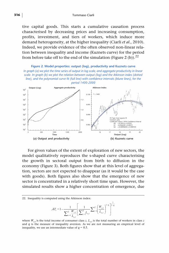
tive capital goods. This starts a cumulative causation processcharacterised by decreasing prices and increasing consumption,profits, investment, and tiers of workers, which induce moredemand heterogeneity, at the higher inequality (Ciarli et al., 2010).Indeed, we provide evidence of the often observed non-linear rela-tion between inequality and income (Kuznets curve) for the periodfrom before take off to the end of the simulation (Figure 2 (b)).22

For given values of the extent of exploration of new sectors, themodel qualitatively reproduces the s-shaped curve characterisingthe growth in sectoral output from birth to diffusion in theeconomy (Figure 3). Both figures show that at this level of aggrega-tion, sectors are not expected to disappear (as it would be the casewith goods). Both figures also show that the emergence of newsector is concentrated in a relatively short time span. However, thesimulated results show a higher concentration of emergence, due

Figure 2. Model properties: output (log), productivity and Kuznets curve

In graph (a) we plot the time series of output in log scale, and aggregate productivity in linear scale. In graph (b) we plot the relation between output (log) and the Atkinson index (dotted line), and the polynomial curve fit (full line) with confidence intervals (blune lines), for the

period 1400-2000

22. Inequality is computed using the Atkinson index:

where Wz,t is the total income of consumer class z, Lz,t is the total number of workers in class zand ϱ is the measure of inequality aversion. As we are not measuring an empirical level ofinequality, we use an intermediate value of ϱ = 0.5.

101

102

103

104

105

106

107

108

109Output (Log)

2000150010005000

Time

1.2

1.0

0.8

Aggregate productivity

(a) Output and productivity

0.100

0.095

0.090

0.085

Atkinson Index

2019181716

Output (Log)

Fit Type: least squares fitFunction: polyCoefficient values ± 95% Confidence Interval

K0 =-0.24514 ± 0.0325K1 =0.036249 ± 0.00371K2 =-0.00096045 ± 0.000105

T > 1400

(b) Kuznets curve

ϱϱ −−

⎥⎥

⎦

⎤

⎢⎢

⎣

⎡

⎟⎟⎠

⎞⎜⎜⎝

⎛− ∑

∑∑

11

1

,

,1=

,1=,

,1=

111=tz

tzZ

ztz

Z

ztz

tzZ

z

t LW

LLWTA


to the fact that we have a fixed number of needs—unlike realsectors, that firms attempt to satisfy as soon as they manage tosearch all sectors: a lower ι would imply a less clustered emergence(see equation 10).

Table 8 in the Appendix reports the results of a Vector Autore-gressive (VAR) analysis on 10 period growth rates, and coefficientsestimated using LAD—with bootstrapped standard errors. The VARshows the relations between output (1), aggregate productivity (2),average price (3), the inverse Herfindahl index (4) and theAtkinson index of inequality (5). Results are in line with theexpected macro dynamics. All variables show a strong cumulativeprocess with one lag. Inequality growth has an immediate positiveeffect on output (1 lag) which becomes negative after three lags.Similarly, an increase in market concentration has an immediatenegative effect on output (1 lag), which becomes positive after twolags. Market concentration also determines an increase in pricesand inequality. The effect of productivity on output in this short-run analysis is captured through price reduction, which has animmediate positive effect on output (1 lag). A detailed discussionon the short and long run dynamics of a previous version of thismodel can be found in Ciarli et al. (2010) and Ciarli et al. (2012).

3.1. Distribution of income across countries

We now move to the analysis of the model for the 2k combina-tions of factors. Each combination of factors in the model can beinterpreted as a different country with different initial conditions.

Figure 3. Sectoral output: industrial production in Britain and simulation results

(a) Sectoral output (log scale) computed by Rostow (1978) (cited in Aoki and Yoshikawa, 2002); (b) sectoral output (log) from the model results with ι = 0.005

(a) Observed

10

9

8

7

6

5

4

Sectoral output (log)

1000800600400200

Time

(b) Simulated

Tommaso Ciarli318

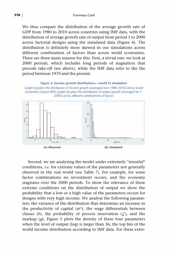
We thus compare the distribution of the average growth rate ofGDP from 1980 to 2010 across countries using IMF data, with thedistribution of average growth rate of output from period 1 to 2000across factorial designs using the simulated data (Figure 4). Thedistribution is definitely more skewed in our simulations acrossdifferent combination of factors than across world economies.There are three main reasons for this. First, a trivial one: we look at2000 periods, which includes long periods of stagnation thatprecede take-off (see above), while the IMF data refer to the theperiod between 1970 and the present.

Second, we are analysing the model under extremely ''stressful''conditions, i.e. for extreme values of the parameters not generallyobserved in the real world (see Table 7). For example, for somefactor combinations no investment occurs, and the economystagnates over the 2000 periods. To show the relevance of theseextreme conditions on the distribution of output we show theprobability that a low or a high value of the parameters occurs fordesigns with very high income. We analyse the following parame-ters: the variance of the distribution that determine an increase inthe productivity of capital (σ a), the wage differentials betweenclasses (b), the probability of process innovation (ζ ), and themarkup (μ). Figure 5 plots the density of these four parameterswhen the level of output (log) is larger than 36, the top bin of theworld income distribution according to IMF data. For these extre-

Figure 4. Income growth distributions—world Vs simulation

Graph (a) plots the distribution of income growth (averaged over 1980-2010) across world economies (Source IMF); graph (b) plots the distribution of output growth (averaged for 1-

2000) across different combinations of factors

05

1015

2025

Den

sity

0 .05 .1 .15Avgr_GDP

(a) Observed

050

100

150

Den

sity

0 .05 .1 .15GdpGAvt

(b) Simulated


mely high levels of output we observe almost one singlecombination of factors: σ a is high with probability 1,23 b is lowwith probability around .95, ζ is high with probability nearly 1and μ is high with probability .95.

The third related reason for the atypical distribution of outputgrowth in our model simulated across the 2k different factor combi-nations is due to the DOE: in Figure 4 (b) we are overlappingdistributions from different data generation processes, where eachcombination of the High and Low values of the parameters repre-sent one process. We show below that some parameters have adramatic effect on the output variables. The distribution of outputvariables differs enormously when these parameters switch fromone state to another. We show this again by comparing the distri-butions in the simulated data. Figure 6 plots the distribution ofoutput for different combinations of some influencing parameterswith High and Low values. It is sufficient to compare the support

23. We denote the low level of the parameters as 0 and the high level of the parameter as 1.

Figure 5. Density of some parameters when Log output > 36

0 denotes a low value of the parameter and 1 denotes a high value. For extremely high values of output the parameters take almost always the same value

0.2

.4.6

.81

Den

sity

0 1

b a

μ

Tommaso Ciarli320

of the total distribution (the last one in the figure, for all values ofthe parameters) with the support of any other distribution whichrepresents a combination of different High and Low values (1,0) ofσ a, μ, ι, v, b. In only one case the support is the same. In mostcases, the support is radically different (lower by a factor 10 or 30).

To sum up, the overall distribution of output variables, such asoutput in the final period, and the average rate of output growthover periods, cannot be approximated satisfactorily by any theore-tical distribution that we know of: the closest would be the Paretodistribution.

The above discussion suggests that economies endowed withdifferent factors that determine the initial structural conditionsand the way in which structural changes in different aspects of theeconomy unfold (or not), experience very different growth paths.By testing extreme values of these conditions we see that a limitednumber of economic aspects—different from the beginning—

Figure 6. Distribution of output (log) for different High and Low values of the parameters

σ a, μ, ι, v, b ; 0 denotes a low value and 1 denotes a high value

0.1

.20

.1.2

0.1

.20

.1.2

0.1

.20

.1.2

5 10 15 20 25 0 10 20 30 5 10 15 20 5 10 15 20 5 10 15 20 5 10 15 20 25

5 10 15 20 25 5 10 15 20 25 6 7 8 9 6 8 10 12 14 6 8 10 12 14 6 8 10 12 14

6 7 8 9 6 8 10 12 14 5 10 15 20 6 8 10 12 14 0 10 20 30 5 10 15 20 25

10 20 30 40 10 20 30 40 50 10 20 30 40 5 10 15 20 25 10 20 30 40 50 0 10 20 30

0 50 100 150 5 10 15 20 25 0 100 200 300 10 20 30 40 0 50 100 150 5 10 15 20 25

0 50 100 150 200 10 20 30 40 0 100 200 300

0, 0, 0, 0, 0 0, 0, 0, 0, 1 0, 0, 0, 1, 0 0, 0, 0, 1, 1 0, 0, 1, 0, 0 0, 0, 1, 0, 1

0, 0, 1, 1, 0 0, 0, 1, 1, 1 0, 1, 0, 0, 0 0, 1, 0, 0, 1 0, 1, 0, 1, 0 0, 1, 0, 1, 1

0, 1, 1, 0, 0 0, 1, 1, 0, 1 0, 1, 1, 1, 0 0, 1, 1, 1, 1 1, 0, 0, 0, 0 1, 0, 0, 0, 1

1, 0, 0, 1, 0 1, 0, 0, 1, 1 1, 0, 1, 0, 0 1, 0, 1, 0, 1 1, 0, 1, 1, 0 1, 0, 1, 1, 1

1, 1, 0, 0, 0 1, 1, 0, 0, 1 1, 1, 0, 1, 0 1, 1, 0, 1, 1 1, 1, 1, 0, 0 1, 1, 1, 0, 1

1, 1, 1, 1, 0 1, 1, 1, 1, 1 Total

Den

sity

Output (log)Graphs by a, μ, , , and b


produce dramatic differences in growth. Also the way that thesedifferent aspects of structural change interact seems to be relevant.

The rest of the paper provides a detailed analysis of the (main,interactive, direct and indirect) effects of these factors on the finaldistribution of output across economies with very different star-ting conditions.

3.2. The factors of structural change

Before analysing factor responses we briefly summarise theeffect of the different factors (parameters) that define the initialstructure of the economy and the dynamics of structural change.24

We group them with respect to the aspects of structural changethey capture directly: product technology, production technology,organisation of production (which refer mainly to the structure ofemployment), income distribution and consumption patterns.Table 7 summarises the ''Low'' and ''High'' values, the main aspectsaffected, and the equation where they appear. Appendix Aprovides detail for the choice of the ''Low'' and ''High'' values.

24. The terms factors and parameters are used interchangeably.

Table 2. Effect of parameters on structural change

A ''+'' indicates that the High value of the parameter induces relatively more structural change

Factor Equation High/Low Low High Main

Economic aspect a

Main indirect aspects a

ι 10 + .001 .3 3 _

v 3 _ 3 50 1 4, 5

b 6 + 1 3 1 4

σ a 17 + .01 .2 2 1

η 22 + .1 3 5 _

ρ = ρ k 8, 15 + .05 .95 3, 2 4

ϑ 11 + .01 10 3 _

ζ 16 + .1 1000 2 1

ς 24 + .05 .9 5 _

μ = μ K 7, 18 + 1.01 2 4 2,3, 1

a 1: Organisation of production; 2: Production technology; 3: Product technology; 4: Income distribution; 5: Consumption patterns

Tommaso Ciarli322

Product technology: ι, ϑ, ρ. All these factors have an effect onthe variety in the final goods market, ι determining the pace atwhich new goods are discovered, ϑ influencing the rate of changein the quality of new goods and ρ altering the resources employedby the firm for the exploration of new goods. ι and ϑ play no otherrole in structural change; ρ influence the distribution of incomethrough the share of profit not redistributed as bonuses and usedfor R&D.

Production technology: σ a, ζ, ρk. Large values of σ a and ζdirectly modify the capital structure of the economy, determiningthe pace at which innovation occurs in the capital goods sector; ρk

has the same effect as ρ in altering the resources devoted to R&D.All three factors have a number of indirect effects on other aspectsof structural change. Similar to ρ, ρk influences the income distri-bution. σ a and ζ in addition to altering the productivity of thefinal goods firm, modify the demand for production factors(labour and capital), affecting firms' labour structure (throughchanges in size). Also, given the different pace at which differentfirms change capital vintages, σ a and ζ change the distribution ofprices in the final goods market, allowing consumers to selectbased on their price preferences.

Organisation of production: v and b. Both parameters definethe way in which a firm is organised: a very low v means that acorporation needs a large number of tiers to organise a small poolof workers, whereas for a large v a single manager can deal with alarge production unit (few changes as the size of the corporationincreases). b tells us simply how the different levels of workers andmanagers are paid (and bonuses are distributed). Both parametershave a strong bearing on the distribution of income as they impli-citly determine the number of income classes (v) and their wageincome. Indeed, v indirectly influences also at least one otheraspect of the economy—changes in consumption patterns—byaltering the pace at which new classes with different consumptionstyles endogenously emerge.

Income distribution: μ, μk. For a small ρ and low capital invest-ment a large μ implies a redistribution of income from allconsumers to higher classes. Indeed, an increase in μ also increasesthe resources available for investment in R&D—thus it increasesthe pace at which product and production technology change.


Finally, differences in markups indicate different market struc-tures, from competitive to oligopolistic.

Consumption patterns: η, ς. High level of both factors inducefaster change in consumption behaviour. A high η implies a veryfast change in expenditure shares from basic needs to the asymp-totic distribution that of the top income centile of UK consumersin 2005. ς changes the consumer preferences in a given classes, fora given expenditure share: a large ς implies that the tolerance forrelatively lower quality (higher price) goods decreases (increases) ata faster rate moving towards the high income classes.

Main and cross effects (without normalising the scale). Asimple graphical analysis explaining the main and the cross effectsof the factors is detailed in Ciarli (2012). Given the scale effect thatunderlies these results, in this paper we focus on the analysis ofvariance (next section). However, a summary of the entity of theeffect of each parameter—which, including its scale, reflects thefact that the parameters represent very different dimensions ofstructural conditions—is a useful complement to an analysis ofvariance that informs on the significance of the effects, but not ontheir magnitude (more in Section 3.4).

For simplicity, we explored two extreme cases, out of the thou-sand possible states of the world analysed in this paper: weanalysed the impact on total output of each factor when all otherfactors are either Low (L) or High (H). We found that, in the casewhere parameters induce low structural change in all dimensionsof the economy, a single factor inducing high structural change issufficient for a strong effect on output. However, this does notapply to all factors and especially not to those that determinechanges in the structure of consumption: the wage multiplier (b)and a higher variance of the productivity shock (σ a) have thestrongest positive effects, followed by the exploration of newgoods (ι); while ρ (share of profits invested in R&D) and μ (mark-up) have the strongest negative impact. On the other hand, if allthe parameters induce high structural change in all dimensions ofthe economy, then just two of the parameters inducing low struc-tural change will have an effect on output (ρ and μ).

We found also that the effect of each parameter in many cases isnot monotonous: the signs of the main effects change if some of

Tommaso Ciarli324

the other factors change from inducing low to inducing high struc-tural change. For example, we analysed the effect of a more or lesscomplex organisational structure (v) under varying structuralconditions, such as wage regimes (b) the likelihood of inventing anew product (ι), and increases in the productivity of capitalvintages (σ a). We found that, while a few factors do not interactwith v – η, ϑ, ς, and ζ, some induce only a level effect—ρ and μ—,ι, b, and σ a change the sign of the effect of v: when they are Low,an increase in v has a mild positive effect on output; when they areHigh, an increase in v has a strong negative effect on output. Thisseems to suggest that highly complex organisations (which requiremany organisational layers, i.e., many employees receiving diffe-rent levels of remuneration, for a given number of workers in thefirst tier) have a positive impact on output growth when marketsdiversify quickly (High ι), when firms can recover the higher orga-nisational costs (reflected in higher consumer prices) throughincreased productivity growth (High σ a), and when wages differbetween organisational layers (b). The rapid vertical growth offirms in fact creates classes of workers with different consumptionshares and different preferences, i.e. consumers that buy moregoods from markets that firms still need to discover (with a High ι)and that are ready to buy goods at higher prices. However, thehigher organisational costs translate into lower aggregate demand.The net effect on output is positive only if either product innova-tion brings results in rapid time to market for goods to satisfy theemerging classes of consumers, or when rapid change in producttechnology compensates for increasing prices (or possibly if bothconditions hold).

3.3. Analysis of variance: the significance of factors' interactions

In order to assess the statistical significance of the effect of eachfactor, and the joint significance of the different factors on output,we run an ANOVA on 20 replicates for each combination of para-meters. The results in Table 3 show that apart from η and ς—respectively the speed of convergence of the expenditure sharesand of the change in the preferences of consumers for a good'scharacteristics—all parameters have a significant main effect, evenwhen tested jointly—when considering the effect of each para-


meter for all possible states of the world (High and Low values ofthe other factors).

Due to the blatant departure from normality of the outputvariable, we check the robustness of the results of the ANOVA bytesting one way differences between the samples defined by theparameters High and Low values with a Kruskal-Wallis (KW) equa-lity of population rank test. The results (see Table 9 in theAppendix B) differ from the ANOVA only with respect to η, whichturns out to have a small but significant negative effect.25 The oneway mean test confirms the results from the graphical analysis:high values of ι, v, b, σ a, ϑ and ζ are associated with a higheroutput; high values of ρ and μ are associated with a lower output;and η and ς have a negligible effect.

This similarity makes us confident that the results of theANOVA for our large sample are informative, and we proceed toanalyse the significance of the first order interactions between allfactors. For instance, as discussed above, ι, b, and σ a modify theeffect of the organisation structure on output. We analyse theseinteractions more systematically in Table 4, which summarises the

Table 3. ANOVA – main effects

Source Partial SS df MS F Prob>F

Model 1.258e+06 9 139790 414.1 0.00

ι 4840 1 4840 14.34 0.00

v 101546 1 101546 300.8 0.00

b 114912 1 114912 340.4 0.00

σ a 260782 1 260782 772.6 0.00

η 691 1 691 2.05 0.15

ρ 481609 1 481609 1427 0.00

ϑ 1399 1 1399 4.150 0.04

ζ 240068 1 240068 711.2 0.00

ς 0.821 1 0.821 0 0.96

μ 52954 1 52954 156.9 0.00

Residual 6.909e+06 20469 337.5

Total 8.168e+06 20479 398.8

Number of obs = 20480; Root MSE = 18.37; R-squared = 0.154; Adj R-squared = 0.154

25. However, note that the KW test is one way.

Tommaso Ciarli326

results of the ANOVA that includes all the main effects and firstorder interactions (i.e. all possible interactions between two diffe-rent factors).

Table 4 confirms the intuition—from the analysis of distribu-tions of output (Figure 6)—that most factors induce structuralchanges that have a significant effect which differs (in size or direc-tion) for different combinations of the other factors, that is, whichis subject to the structural changes induced by the other factors. Inother words, the different dimensions of structural changesinduced by the factors, significantly interact in determining theaggregate behaviour of the economy.

For example, what would be the effect on growth of increasingthe opportunities for R&D in the capital sector (σ a)? As shown inTable 3, σ a alone has an apparent impact on output. However,Table 4 shows that the role of the production technology cruciallydepends on many other structural aspect of the economy, such asthe organisation of production (v, b), and especially the share ofprofits invested in R&D and its effectiveness on the innovationresult (ρ, ζ ). Its strong effect on output is relatively independent ofthe introduction of product variety in the consumer market (ι, ϑ)and of the structure of demand for more variety (η, ς).

To better discriminate among the different aspects of the struc-ture of an economy, in the next section we perform a regressionanalysis that allows us to quantify the effect of factors across designs.

Table 4. ANOVA – first order interactions

(1) (2) (3) (4) (5) (6) (7) (8) (9) (10)

ι v b σ a η ρ ϑ ζ ς μ

ι 0

v ** ***

b *** *** ***

σ a 0 *** *** ***

η ** 0 0 0 0

ρ *** *** *** *** 0 ***

ϑ 0 0 0 0 0 ** 0

ζ ** *** *** *** 0 *** 0 ***

ς 0 *** * 0 0 0 * 0 0

μ ** *** *** *** 0 *** 0 *** ** ***

Note: Values on the diagonal refer to the factor main effect. ***Prob > F < 0.01; **Prob > F < 0.05; *Prob > F < 0.1; 0: Prob > F > 0.1


3.4. The relative influence of the different aspects of structural change

We run quantile regressions (with bootstrapped standard errors)to estimate the relative impact and significance of each factor andtheir first order interactions on output. We distinguish betweendirect and indirect impact: Table 5 reports estimates for the factors(1), for a number of control variables, most of which are correlatedto the factors (2), and for the parameters when the least correlatedcontrol variables are included—a sort of reduced form of the model(3).26 Table 6 reports the estimates for the parameters and theirfirst order interactions, with and without control variables (respec-tively bottom-left and top-right triangular matrix).

On average, when abstracting from the different structuralchange regimes (column 2), the model shows that aggregate labourproductivity (A)—measured as output per worker—is strongly andpositively correlated to output as well as average expenditure onR&D (across firms and time periods) (R). As noted elsewhere (Ciarliet al., 2010; Ciarli and Lorentz, 2010), product variety (averagedover the full period)— σ q and σ p, respectively for quality andprice—and the selection that they enable also positively affectoutput; but their effect is weak and non-significant when control-ling for inequality and productivity, which is the prime cause ofprice differences. Inequality (AT), averaged over the whole period,has an overall negative effect on output.

With reference to factors (column 1), ρ and μ determine struc-tural changes with the strongest (negative) effect on output,followed by σ α, ι and b. Related to σ α, ζ also has a positive andsignificant effect. The least relevant are the structural changesinduced by v, ς (positive) and η (negative).

The factors determining structural change also influence thedynamics of a large number of variables. Therefore, the estimatedeffect of a variable on output (Table 5) is likely to differ for diffe-rent levels of the parameters. Likewise, the use of control variablesin the estimation of parameters allows us to estimate the directeffect of the factors on output, depurated from the indirect effectthrough the control variables.

26. The estimated sample is the result of the simulations for the last period for 20 replicates ofeach combination of parameters.

Tommaso Ciarli328

Table 5. The relative impact of factors and main variables on outputLAD estimates with s.e. obtained from bootstrapping (400); the dependent variable is

(Log) output

(1) (2) (3)

Variables Factors Contr Var F & CV ι 0.692*** 1.063***

(0.056) (0.071)

v 0.009*** -0.012***

(0.000) (0.000)

b 0.107*** -0.061***

(0.008) (0.007)

σ a 3.242*** 0.966***

(0.088) (0.083)

η -0.023*** -0.016***

(0.006) (0.004)

ρ -4.900*** -3.947***

(0.024) (0.036)

ϑ 0.013*** 0.003**

(0.002) (0.001)

ζ 0.001*** 0.000***

(0.000) (0.000)

ς 0.040** 0.021*

(0.019) (0.011)

μ -9.330*** -9.510***

(0.018) (0.021)

A 1.201*** 2.900***

(0.071) (0.057)

A T -3.809*** 3.523***

(1.109) (0.109)

σp 0.119* -0.092***

(0.065) (0.004)

σq 0.001 0.000***

(0.001) (0.000)

R 0.779***

(0.048)

Constant 28.301*** 12.944*** 29.424***

(0.043) (0.380) (0.075)

Observations 20,480 20,480 20,480

Pseudo R2 0.43 0.09 0.48

Standard errors in parentheses *** p<0.01, ** p<0.05, * p<0.1


To better show this interaction between factors and economicvariables, Figure 7 plots the relation between an independentvariable, aggregated productivity, and output (Log), for differentvalues of the parameters. In panel a no restrictions on parametersare imposed, and the relation between the two variables is distinctlynon-linear and non monotonic. More importantly, panel a suggeststhat the relation between productivity and output could be reducedto different functional forms, depending on the combination offactors. In panel b we restrict all factors to either the high or the lowvalue: aggregate productivity does not show any significant effecton output under either condition. Results are different if we allowthe parameters that are strongly related to aggregate productivity tofluctuate. In panel c all factors are either high or low, except for ρ,which takes both values. Although the relation between the twovariables is not so clear cut, the scale is radically different—thesmall dot in the bottom left of panel c is the flat relation that weobserve at the bottom right side of panel b. Alternatively, for diffe-rent levels of markup (μ) the relation turns from null to positive, forhigh values of all other parameters (panel d).

Returning to Table 6, column (3) shows estimates for the directeffects of the factors and for the effect of the least correlatedvariables. First, the sign of the two factors defining the organisa-tion of production are inverted. A high v means a lower number of(organisational) workers per good produced, increasing labourproductivity. When we control for labour productivity, though,the lower number of tiers for a given number of shopfloor workersreduces the pace at which firms grow in size and diversify byadding different levels of workers and managers (see Eq. 3 and 14).The effect on structural change is a slower increase in the aggregatedemand and its variety, and a negative impact on output growth.While large wage differentials (b) increase inequality, which has anegative effect on output, ceteris paribus, but which in our model isassociated also with larger aggregate demand (Eq. 20); thus theinverted sign of AT when controlling for the factors. Second, thedirect effect of σ α is strongly reduced when controlling for aggre-gate productivity. Third, the estimated effect of a few variableschange their sign and significance as we control for differentcombinations of the factors determining structural changes.

Tommaso Ciarli330

As already mentioned, the effect that each of the factors induceson structural change depends also on other structural aspects. Therelevance of the interaction among several factors is established inthe results of the quantile regression where all first order interac-tions are estimated together with the main effects, with andwithout the control variables Table 6. We estimate the effect of thehigh value of factors, the low value being the reference case. Esti-mates without control variables are reported in the top-righttriangular matrix and those that include control variables arereported in the bottom-left triangular matrix. On the diagonal wereport the main effects (when controlling for interactions). In thefollowing we discuss the estimates obtained when including thecontrol variables (bottom-left triangle). First, the results in Table 6show that the main effects are strongly significant, despite theinclusion of the interaction terms. Second, most of the first orderinteraction terms are also significant, particularly when they

Figure 7. Aggregate productivity Vs output (Log)

T=2000, aggregate productivity on the x-axis and output on the y-axis

050

100

150

200

250

lnG

dp

0 20 40 60 80 100AggProd

(a) No restrictions on factors6

810

1214

16

lnG

dp

.6 .8 1 1.2 1.4AggProd

All Low All High

(b) All factors Low or High

010

2030

lnG

dp

0 20 40 60 80 100AggProd

All Low All High

(c) All factors Low or High, except ρ

510

1520

lnG

dp

.6 .8 1 1.2 1.4AggProd

All Low All High

(d) All factors Low or High, except μ


include a factor shown to have a significant main effect. Weproceed by discussing the effect of the different aspects of struc-tural change, following the classification in Table 2.

Product technology: ι, ϑ, ρ. The effect on output of rapid emer-gence of new sectors is large and positive on average, but is alwaysnegative when other factors induce strong structural change (withthe exception of the factors defining consumption patterns, η andς). That is, for fast changes in consumption shares and/or prefe-rences the high level of ι has a (weakly) significant positive effect.We note also that the interaction between the two main factors ofproduct technology, ι and ϑ—respectively needs and quality—isnot significant.

Table 6. LAD regression – the effect of first order interactions on outputThe top-right triangular matrix shows estimates without control variables; the bottom-left

triangular matrix shows estimates with control variables. The dependent variable is output (Log)

(1) (2) (3) (4) (5) (6) (7) (8) (9) (10)

ι v b σ a η ρ ϕ ζ ς μ ι

1.51 0.16 -0.09 -0.31 -0.01 -0.55 0.03 -0.18 0.04 -0.97

1.38

v0.28 0.33 -0.95 0.69 0.23 -0.56 -0.08 0.62 0.12 0.20

-0.81 b

-0.10 -0.16 1.14 -0.24 -0.15 0.11 -0.05 -0.34 -0.28 0.10

0.10 σa

-0.37 0.68 -0.34 1.51 0.00 -1.58 0.09 2.26 -0.12 -0.73

1.39 η

0.04 0.28 -0.21 -0.03 -0.18 0.00 -0.02 -0.04 0.08 0.10

-0.26 ρ

-0.52 -0.35 0.31 -1.00 0.00 -0.56 -0.57 -1.42 0.01 -2.51

-0.98 ϑ

-0.05 0.01 -0.08 0.18 0.00 -0.61 0.55 0.10 0.20 -0.17

0.58 ζ

-0.14 0.42 -0.34 1.18 0.03 -0.88 0.08 1.24 -0.14 -0.39

1.05 ς

0.05 0.23 -0.20 -0.03 0.11 -0.06 0.20 -0.12 0.17 -0.37

0.10 μ

-0.98 -0.24 0.37 -1.27 0.12 -1.61 -0.56 -0.96 -0.31 -6.06

-6.22

Note: Values on the diagonal refer to the factor main effect. Standard errors computed with 400 bootstraps. Refe-rence case is the low value of factors.

p<0.01 p<0.05 p<0.1

Tommaso Ciarli332

Production technology: σ a, ζ, ρK. The main factors that affectchanges in production technology, σ α and ζ, also have a pervasiveeffect, interacting with all other aspects of structural change,except those that define changes to consumption patterns. Inparticular, the relation with organisational factors is negative: foran increase in organisational complexity—i.e. reduction in v—orwage differences, fast changes in technology reduce outputgrowth. Taken together with the negative sign of the interactionwith ρ, this result suggests that rapid changes in the productivitycomponent of capital have a negative impact on output in thepresence of high markups, large wage differences and multipleorganisational tiers which amplify wage differences. In otherwords, economies that experience fast changes in productivitygrow at a lower pace if the structure imposes as well an unequaldistribution of the productivity gains. The interaction withproduct technology is negative with respect to the discovery ofnew sectors, and positive with respect to changes in productquality. Finally, the two main factors affecting changes in produc-tion technology— σ a and ζ —are strongly and positively related toincreased output.

Organisation of production: v and b. A large number of layersrequired to manage an organisation (low v) and large wage diffe-rences (b) between these layers have a negative impact in thepresence of strong structural change in all other aspects exceptthose affecting income distribution, μ. Even in the presence ofrapid changes in consumption patterns, higher wage inequalityreduces output growth.

Income distribution: μ, μk. A large markup generating highprofits in our model has a negative impact under almost all aspectsof strong structural change, except for the organisational aspectsdiscussed above, and changes in expenditure shares.

Consumption patterns: η, ς. As already noted, the factorsdetermining structural changes in consumption play a minor rolein output growth. The interactions with many other aspects ofstructural change are not significant: the main effects of consump-tion patterns are visible when structural change occurs in producttechnology and the distribution of income. Indeed, the emergenceof new products is a requirement for changes in consumption to


have a role on output. The two main aspects of consumptionpatterns, η and ς interact positively.

4. Discussion and conclusions

A large wealth of research has investigated why regions startingfrom a similar level of output grow so differently through time.Which are the initial apparently small differences that diverge somarkedly? In this paper we build on the idea that the initial diffe-rences that determine growth divergence are those that define thestructure of an economy and the way in which this evolvesthrough time. We maintain that structural change occurs in diffe-rent aspects of the economy, such as the structure of production,consumption, labour organisation and income distribution. Thesedifferent dimensions of structural change interact in a continuousevolutionary process, and are not independent from the growthpattern. For example, one could not think at the industrial revolu-tion without considering aspects such as changes in knowledgeand technology, changes in the patterns of consumption, changesin trade patterns and extraction of resources through colonialpower, and institutional changes. In turn, changes in knowledgeand technology may be driven by changes in the demand, as wellas by changes in labour relations (e.g. increase in the cost oflabour). Similarly, changes in transportation and military techno-logies are not independent from changes in technologicalknowledge. Changes in consumption patterns are also related toincreased trade. And so on.

We propose a model of the microeconomic dynamics of struc-tural change and their interactions, abstracting from theinstitutional aspects. The model defines the following relatedaspects of structural change: organisation of production, techno-logy of production and the emergence of new sectors on the supplyside, and income distribution and consumption patterns on thedemand side. Ten different parameters (factors) in the modelaccount for these five dimensions of structural change.

In this paper we simply investigate the relative importance ofeach aspect of structural change in economic growth. We alsoacknowledge that some of these aspects are likely to have a sizeableimpact on economic growth only when complemented by other

Tommaso Ciarli334

aspects of structural change. For example, changes in consumptionpatterns may not occur if there is no change in the sectoral compo-sition of the economy, or if there is no change in wages. Wetherefore use the model to study the interaction among the diffe-rent aspects of structural change, analysing factors' interactions.

To do so, for each of the ten parameters defining the differentaspects of structural change we assign a high and a low value,respectively identifying large and small structural change as theeconomy grows. We then define a DOE that accounts for allpossible combinations of the parameters' high and low values.

In other words, we define 210 different economies, all startingfrom the same initial conditions except for one of the aspects ofstructural change. On one extreme we have an economy that expe-riences negligible structural changes in all economic aspects, andon the other extreme an economy that experiences large structuralchanges in all economic aspects. In between are all other possiblecombinations. We study the impact of the five different aspects ofstructural changes with an analysis of variance, and running quan-tile regressions on the cross-design—cross-country—sample.

We find that almost all aspects of structural change are signifi-cant determinants of the differences in the growth rate of outputacross designs, but their magnitude varies substantially. Incomedistribution, rate of change in production technology and theemergence of new sectors, explain a great deal of output growthdifferences, changes in consumption patterns—shares and prefe-rences—are barely significant, and changes in the organisation ofproduction—organisation and compensation of labour—lay inbetween. Moreover, the most relevant factors of structural changeplay a determinant role even in the presence of negligible struc-tural changes in all other economic aspects. While the oppositecase is rarely true: the output growth of economies that are set toexperience large structural changes in all aspects except for one, isnot affected if one of the changes is only negligible.

Concerning the complementarity among different aspects, wefind that most factors of structural change strongly interact. This isan extremely relevant result suggesting that we should alwaysaccount for a large number of economic aspects to understandlong term patterns of across-countries divergence. For example, we


find that changes in the composition of sectors available in themarket become more relevant when consumption patterns alsoexperience strong structural changes. Or, technological progress isstrongly relevant, but quick technological advances have a nega-tive effect on output growth when they are accompanied bystructural changes in the organisation of labour that leads to largeinequality among a large number of emerging classes. In otherwords, economies that experience fast changes in productivity,grow at a lower pace if the structure imposes as well an unequaldistribution of the productivity gains among workers.

Taken together, the model and the analysis of the experimentaldesign we proposed in this article clearly show that to explain longterm growth we need to look at the way in which a large number ofstructural changes interact at the microeconomic level. It is notunlikely to find that some aspects of structural change were deter-minant for some regions, and detrimental for others (such as thepay structure at the beginning of the industrial revolution inEurope). Moreover, while some of the interactions between thedifferent aspects are relatively known, many interactions insteadsuggest avenues for future research on the relation between growthand structural change.

For example, the results show that inequality is related tooutput growth in a number of different ways through the differentaspects of structural change. This is in line with the lack of agree-ment, on theoretical and empirical grounds, on the relationbetween inequality and GDP growth (Aghion et al., 1999; Eicherand Turnovsky, eds, 2007). In our model the effect of inequality onoutput is transmitted through the aggregate demand. For example,higher wage inequality per se increases the overall amount ofresources allocated to consumers, as well as more complex organi-sation of firm labour (low v). But the relation between inequalityand output when we do not control for structural parameters (aresult biased by omitted variables) is negative. This correlationsimply says that in stagnating economies, due to a lack of demand,there is no investment in capital goods and all profits are redistri-buted to managers: low growth induces inequality. Althoughinstitutions have no role in our model, this result is in line with theliterature that shows the relevance of elite behaviour in countrieslong run development (Acemoglu et al., 2005). While an economy

Tommaso Ciarli336

growing rapidly also generates some inequality, due to the hierar-chical structure of firms, this same non-linear increase in vacanciesthat accompanies an increase in demand generates even moregrowth and demand. This is amplified by the size of wages, i.e.consumable income. However, as noted elsewhere (Ciarli et al.,2010), it is the overall demand that counts in our model, and nothow it is redistributed, given that we assume that all classes havethe same propensity to consume their income. Here we simplyobserve that growing firms generate more demand; and differentwage classes consume a different set of goods. However, given theminor role played by demand side factors in our model, we canmake no judgement on what would be the best way to redistributesalaries. What seem to be essential from analysing the model dyna-mics is the selection of firms by consumers, either because theydifferentiate on price (low income) or on quality (top incomes).And because of the pyramidal structure of the firm, the price selec-tion by the large population of shop-floor workers seems essentialin facilitating the transition from low to exponential growth.Finally, large profit shares in the form of large mark-up have theopposite effect on real demand, through an increase in prices, witha negative impact on output growth. We plan to focus more on therelation between the different aspects of inequality and outputgrowth in future research, exploiting the panel structure of thesimulation data.

Among the implication for future research with this and similarmodels, two limitations in the analysis of this paper suggest twofuture steps. First, here we do not consider the deeper determinantsof the initial differences in the factors that determine structuralchange, which are mainly related to institutional aspects—in abroad sense—and to the intricate relation between knowledge,technology, and institutions. In future work we want to build onthe sizeable literature that uses the case of the industrial revolu-tion(s) to investigate the relations between knowledge,technology, and institutions to shed more light on the origins ofthe structural difference that we model here. Second, havingstudied here which are the most relevant aspects in determiningthe output response with a simple DOE, the next step is to focus onthose aspects and analyse whether their effect on output is linearand monotonous, as assumed in the DOE. Previous work suggests


that it is not (Ciarli and Lorentz, 2011; Ciarli et al., 2012). Of parti-cular importance is the relation between the various componentsof inequality, labour organisation and output growth. Moreover,we plan to study how different aspects of structural change modifytheir effect through time, exploiting the panel structure of thedata. Finally, one can exploit these same results to simplify themodel reducing the number of parameters and behavioural details.With reference to the model presented here, we plan to simplifypurchase behaviour to a completely adaptive demand behaviour.More in general, it seems like a good strategy to start with highlycomplex agent based models, thoroughly analyse the most rele-vant aspects with an appropriate DOE, and learn from the analysishow to simplify the model, stylising the aspects that have littleinfluence on the outputs.

References

Acemoglu D., S. Johnson, and J. A. Robinson, 2005. “Institutions as afundamental cause of long–run growth.” In Philippe Aghion andSteven N. Durlauf, editors, Handbook of Economic Growth, volume 1A ofEconomic handbooks, chapter 6, pages 385–472. Elsevier.

Aghion P. and P. Howitt, 1998. Endogenous Growth Theory, Vol. 1 of MITPress Books, Cambridge, MA: The MIT Press, December.

Aghion P., E. Caroli, and C. García-Peñalosa, 1999. “Inequality andeconomic growth: The perspective of the new growth theories.”Journal of Economic Literature, 37(4):1615–1660, December.

Amendola M., and J.-L. Gaffard, 1998. Out of Equilibrium. Oxford: OxfordClarendon Press.

Andrews M. J., S. Bradley, D. N. Stott, and R. Upward, 2008. “Successfulemployer search? an empirical analysis of vacancy duration usingmicro data.” Economica, 75(299):455–480.

Aoki M., and H. Yoshikawa, 2002. “Demand saturation–creation andeconomic growth.” Journal of Economic Behavior & Organization, 48(2):127–154.

Atkinson A. B., 2007. “The distribution of earnings in oecd countries.”International Labour Review, 146(1-2):41–60.

Bassin W. M., M. T. Marsh, and S. Walitzer, 2003. “A macroeconomicanalysis of inventory/sales ratios.” Journal of Business & EconomicsResearch, 1(10):37–45.

Tommaso Ciarli338

Baumol W. J., 2010. “The two-sided cost disease and its frightening conse-quences.” In F. Gallouj and F. Djellal, editors, The handbook onInnovation and Services. Cheltenham: Edward Elgar.

Berg M., 2002. “From imitation to invention: creating commodities ineighteenth-century Britain.” Economic History Review, 55(1):1–30.

Blanchard O. J., 1983. “The production and inventory behavior of theamerican automobile industry.” Journal of Political Economy, 91(3):pp. 365–400.

Blanchflower D. G. and A. J. Oswald, 2006. The wage curve: An entry writtenfor the new palgrave, 2nd edition. IZA Discussion Paper 2138, Bonn, May.

Blinder A. S., 1982. “Inventories and sticky prices: More on the microfoun-dations of macroeconomics.” American Economic Review, 72(3):334–348.

Blinder A. S., 1991. “Why are prices sticky? preliminary results from aninterview study.” American Economic Review, 81(2):89–96.

Boeri, T., 2012. “Setting the minimum wage.” Labour Economics 19(3):28–290.

Bottazzi, G. and M. Grazzi, 2010. "Wage-size relation and the structure ofwork—force composition in Italian manufacturing firms," CambridgeJournal of Economics, 34 (4):649–669.

Buchanan M., 2009. “Economics: Meltdown modelling. could agent-basedcomputer models prevent another financial crisis?.” Nature, 460:680–682.

Celsi R. L., and J. C. Olson, 1988. “The role of involvement in attentionand comprehension processes.” Journal of Consumer Research,15(2):210–224.

Chiarella C., P. Flaschel, G. Groh and W. Semmler, 2000. Disequilibrium,growth, and labor market dynamics: macro perspectives. Springer,Heidelberg.

Ciarli T., A. Lorentz, M. Savona, and M. Valente, 2010. “The effect ofconsumption and production structure on growth and distribution. Amicro to macro model.” Metroeconomica, 61(1):180–218.

Ciarli T., A. Lorentz, M. Savona, and M. Valente, 2012. “The role of tech-nology, organisation, and demand in growth and incomedistribution.” LEM Working Papers 2012/06, Laboratory of Economicsand Management, San’Anna School of Advanced Studies, Pisa.

Ciarli T. and A. Lorentz., 2010. “Product variety and changes in consump-tion patterns: The effects of structural change on growth.” Workingpaper mimeo, Max Planck Institute of Economics.

Ciarli T., and A. Lorentz, 2011. “Product variety and economic growth.trade off between supply and demand dynamics.” Working papermimeo, Max Planck Institute of Economics.


Ciarli T., 2012. “Structural interactions and long run growth: An applica-tion of experimental design to agent based models.” Papers onEconomics and Evolution 1206, Max Planck Institute of Economics,Evolutionary Economics Group, Jena.

Clark C., 1940. The Conditions of Economic Progress. MacMillan, London.

Coad A. and R. Rao, 2010. “Firm growth and r&d expenditure.” Economicsof Innovation and New Technology, 19(2):127–145.

Coelli T., E. Grifell-Tatjé, and S. Perelman, 2002. “Capacity utilisation andprofitability: A decomposition of short-run profit efficiency.” Interna-tional Journal of Production Economics, 79(3):261–278.

Colander D., P. Howitt, A. Kirman, A. Leijonhufvud, and P. Mehrling,2008. “Beyond DSGE models: toward an empirically based macroeco-nomics.” American Economic Review, 98(2):236–240.

Cooper, Russel W and John C. Haltiwanger, "On the Nature of CapitalAdjustment Costs," Review of Economic Studies, 2006, 73(3):611–633.

Criscuolo C., 2000. "Employer Size - Wage Effect: A Critical Review and anEconometric Analysis." SSRN eLibrary.

Dasgupta S., and A. Singh, 2005. “Will services be the new engine ofindian economic growth?” Development and Change, 36(6):1035–1057.

Davis S. J., R. J. Faberman, and J. C. Haltiwanger, 2010. “The establish-ment-level behavior of vacancies and hiring.” Working Paper 16265,National Bureau of Economic Research.

Dawid H. and W. Semmler, 2010. “Introduction to the special issue:Computational perspectives in economics and finance: Methods,dynamic analysis and policy modeling.” Journal of Economic Dynamicsand Control, 34(9):1529–1530.

Delli Gatti D., E. Gaffeo, and M. Gallegati, 2010. “Complex agent-basedmacroeconomics: a manifesto for a new paradigm.” Journal of EconomicInteraction and Coordination, 5:111–135.

Desmet K., and S. L. Parente, 2009. “The evolution of markets and therevolution of industry: A quantitative model of england’s develop-ment, 1300-2000.” Working Papers 2009-06, Instituto Madrileño deEstudios Avanzados (IMDEA) Ciencias Sociales.

DeVaro J., 2005. “Employer recruitment strategies and the labor marketoutcomes of new hires.” Economic Inquiry, 43(2):263–282.

De Loecker J., and F. Warzynski, 2009. “Markups and firm-level exportstatus.” NBER Working Papers 15198, National Bureau of EconomicResearch, Inc.

Dietrich A., and J. J. Krüger, 2010. “Numerical explorations of the ngai-pissarides model of growth and structural change.” Working Papermimeo, Darmstadt University of Technology.

Tommaso Ciarli340

Doms M. and T. Dunne, 1998. "Capital Adjustment Patterns in Manufactu-ring Plants," Review of Economic Dynamics, 1, 409–429.

Dosi G., G. Fagiolo, and A. Roventini, 2010. “Schumpeter meeting keynes:A policy–friendly model of endogenous growth and business cycles.”Journal of Economic Dynamics and Control, 34:1748–1767.

Dosi G., Marengo L., and C. Pasquali, 2006. “How much should societyfuel the greed of innovators?” : On the relations between appropri-ability, opportunities and rates of innovation. Research Policy,35(8):1110 – 1121.

Eicher T. S. and S. J. Turnovsky, editors, 2007. Inequality and Growth. Theoryand Policy Implications. CESifo Seminar Series. MIT Press.

Fabiani S., M. Druant, I. Hernando, C. Kwapil, B. Landau, C. Loupias, F.Martins, T. Mathä, R. Sabbatini, H. Stahl, and A. Stokman, 2006. “Whatfirms’ surveys tell us about price-setting behaviour in the euro area.”International Journal of Central Banking, 2:3–47.

Fisher A. G. B., 1939. “Production, primary, secondary and tertiary.”Economic Record, 15(1):24–38.

Fraumeni B., 1997. “The measurement of depreciation in the u.s. nationalincome and product accounts.” Survey of current business, Bureau ofEconomic Analysis, July.

Galor O., 2010. “The 2008 lawrence r. klein lecture comparative economicdevelopment: Insights from unified growth theory.” InternationalEconomic Review, 51(1):1–44.

Gervais M., and P. Klein, 2010. “Measuring consumption smoothing incex data.” Journal of Monetary Economics, 57(8):988–999.

Gigerenzer G., 1997. "Bounded Rationality: Models of Fast and Frugal Infe-rence." Swiss Journal of Economics and Statistics, 133 (2).

Gigerenzer G., and R. Selten (editors), 2001. Bounded rationality: The adap-tive toolbox, Cambridge, MA: MIT Press.

Hall S., M. Walsh, and A. Yates, 1997. “How do uk companies set prices?”Working Paper 67, Bank of England.

Idson T. L. and W. Y. Oi, 1999. "Workers Are More Productive in LargeFirms." American Economic Review, 89 (2, Papers and Proceedings), 104–108.

Oliveira M. J., S. Scarpetta, and D. Pilat, 1996. “Mark-up ratios in manufac-turing industries: Estimates for 14 oecd countries.” OECD EconomicsDepartment Working Papers 162, OECD Publishing.

Jung P., and M. Kuhn, 2011. “The era of the u.s.-europe labor marketdivide: what can we learn?” MPRA Paper 32322, University Library ofMunich, Germany, July.

Kaldor N., 1957. “A model of economic growth.” Economic Journal,December:65–94.


King R. G. and R. Levine, 1994. “Capital fundamentalism, economicdevelopment, and economic growth.” Policy Research Working PaperSeries 1285, The World Bank, April.

Kleijnen J. P. C., S. M. Sanchez, T. W. Lucas, and T. M. Cioppa, 2005.“State-of-the-art review: A user’s guide to the brave new world ofdesigning simulation experiments.” INFORMS Journal on Computing,17(3):263–289, Summer.

Kleijnen J. P. C., 2005. “Simulation experiments in practice: statisticaldesign and regression analysis.” Journal of Simulation, 2(1):19–27.

Krueger D. and F. Perri, 2005. “Understanding consumption smoothing:Evidence from the u.s. consumer expenditure data.” Journal of the Euro-pean Economic Association, 3(2/3):340–349.

Kuznets S., 1973. “Modern economic growth: Findings and reflections.”The American Economic Review, 63(3):247–258.

Langbraaten N., E. W. Nordbo and F. Wulfsberg, 2008. “Price-settingbehaviour of norwegian firms - results of a survey.” Norges BankEconomic Bulletin, 79(2):13–34.

Law A. M., 2004. “Statistical analysis of simulation output data: The prac-tical state of the art.” In Winter Simulation Conference, pages 67–72.

LeBaron B. and L. Tesfatsion, 2008. “Modeling macroeconomies as open-ended dynamic systems of interacting agents.” American EconomicReview, 98(2):246–50, May.

Leijonhufvud A. 2006. “Agent-based macro.” Volume 2 of Handbook ofComputational Economics, pages 1625–1637. Elsevier.

Llerena P. and A. Lorentz, 2004. “Cumulative causation and evolutionarymicro-founded technical change: On the determinants of growth ratesdifferences.” Revue Economique, 55(6):1191–1214.

Lydall H. F., 1959. “The distribution of employment incomes.” Economet-rica, 27(1):110–115.

Maddison A., 2001. The World Economy: A Millennial Perspective. OECD,Paris.

Marchetti D. 2002. “Markups and the business cycle: Evidence from italianmanufacturing branches.” Open Economies Review, 13(1):87–103.

Matsuyama K., 2008. “Structural change.” In Steven N. Durlauf andLawrence E. Blume, editors, The New Palgrave Dictionary of Economics.Palgrave Macmillan, Basingstoke.

McCloskey D. N., 2009. “Science, bourgeois dignity, and the industrialrevolution.” MPRA Paper 22308.

Mokyr J., 2002. The gifts of Athena: historical origins of the knowledgeeconomy. Princeton: Princeton University Press.

Moneta A., D. Entner, P. Hoyer, and A. Coad, 2010. “Causal inference byindependent component analysis with applications to micro- and

Tommaso Ciarli342

macroeconomic data.” Jena Economic Research Papers 2010-031, Jena:Friedrich Schiller University Jena and Max Planck Institute ofEconomics.

Montgomery D. C. 2001. Design and Analysis of Experiments. John Wiley &Sons, New York, 5 edition.

Nadiri M. I., and I. R. Prucha, 1996. “Estimation of the depreciation rate ofphysical and r&d capital in the u.s. total manufacturing sector.”Economic Inquiry, 34(1):43–56.

Nelson R. R., and Winter S.G., 1982. An Evolutionary Theory of EconomicChange. Cambridge, MA: Harvard University Press.

Nickell S., L. Nunziata, 2002. Wolfgang Ochel, and Glenda Quintini. “Thebeveridge curve, unemployment and wages in the oecd from the 1960sto the 1990s.” Working paper, CEPR, LSE, London.

Nijkamp P., and J. Poot. 2005. “The last word on the wage curve?” Journalof Economic Surveys, 19(3):421–450.

Office for National Statistics, 2006. Expenditure and food survey, 2005-2006.Technical report, Office for National Statistics, Department for Envi-ronment, Food and Rural Affairs.

Rostow W.W., 1978. The World Economy: History and Prospect. Austin:University of Texas Press.

Ryoo J., and S. Rosen, 1992. “The market for engineers.” Working Paper83, University of Chicago - George G. Stigler Center for Study ofEconomy and State, Chicago.

Saviotti P. P., and J.-L. Gaffard, 2008. “Preface for the special issue of jee on’innovation, structural change and economic development’.” Journal ofEvolutionary Economics, 18(2):115–117.

Silverberg G. and B. Verspagen, 2005. "Evolutionary Theorizing onEconomic Growth." in Kurt Dopfer, ed., The Evolutionary Foundationsof Economics, Cambridge: Cambridge University Press, chapter 16,pp. 506–539.

Simon H. A., 1957. “The compensation of executives.” Sociometry,20(1):32–35, March.

Teo E., S. M. Thangavelu, and E. Quah, 2004. “Singapore’s beveridge curve:A comparative study of the unemployment and vacancy relationshiofor selected east asian countries.” Economic Survey of Singapore SecondQuarter, Ministry of Manpower.

U.S. Census Bureau, 2008. Manufacturing and trade inventories and sales.http://www.census.gov/mtis/www/mtis.html

Wall H. J. and G. Zoega, 2002. “The british beveridge curve: A tale of tenregions.” Oxford Bulletin of Economics and Statistics, 64(3):257–276.

Zeithaml V. A., 1988. “Consumer perceptions of price, quality, and value:A means-end model and synthesis of evidence.” The Journal ofMarketing, 52(3):2–22.

http://www.census.gov/mtis/www/mtis.html


Appendix

A. Experimental design

The choice of limit values

The ''Low'' and ''High'' values of the factors analysed in thispaper were chosen following three criteria: (i) the minimum ormaximum possible values (when a limit exists, such as in shares):in this case we selected values that approximate the extremes. (ii)We made reference to the empirical evidence, and chose valuesbelow the minimum observed for ''Low'', and values above themaximum observed for High. Or (iii) when the factors have beentested in previous work (for a large number of values) we used thevalues below/beyond which the factor did not show to have asignificant effect. The mix of these criteria makes the choice of the''Low'' and ''High'' values in this paper quite robust and meanin-gful—we do not see many other options for this type of work.

Table 7. Choice of limit values of factorsThe ''Low'' and ''High'' values of the factors are chosen with respect to available empirical

evidence and/or within theoretically possible and meaningful values.

Factor Low High

ι Approximates the minimum No significant effect found above 0.2 when we analyse a large number of values between 0 and 10 (Ciarli and Lorentz, 2011)

ν Minimum postulated in Lydall (1959); Simon (1957)

Far above the max postulated in Lydall (1959); Simon(1957) and very marginal effect observed beyond 15 (Ciarli et al. 2012)

b The minimum Above the maximum postulated by Lydall (1959); Simon (1957)

σa Approximates the minimum Maximum valued used in Ciarli et al.( 2012): an extremely large number for the time frame postulated here

ηClose to the minimum (to allow for some changes in consumption pat-terns)

Well beyond the theoretical maximum

ρ = ρk Approximates the minimum share Approximates the maximum share

ϑ Approximates the minimum value No significant effect found above 2 when we analyse a large number of values between 0 and 10 (Ciarli and Lorentz, 2011)

ξ Close to the minimum Close to max probability (also for small level of R&D investment)

ς Approximates the minimum share Approximates the maximum share

μ = μ K Approximates the minimum Well beyond observed evidence (De Loecker and Warzinski, 2009; Joaquim Oliveira et al., 1996; Marchetti, 2002)

Tommaso Ciarli344

B. Tables

Table 8. Vector autoregression analysis of the main macro variables

Results from LADestimates of 10 periods growth rates, and bootstrapped standard errors (400). (1) ΔY: output growth; (2) ΔA: Aggregate productivity (3) ΔP: price; (4) ΔIHI: inverse Herfindhal Index (5) ΔAT: Atkinson inequality index. The numbers in parenthesis indicate the

number of lags

(1) (2) (3) (4) (5)

Variables ΔY ΔΑ ΔP ΔIHI ΔAT

ΔY (1) 0.986*** -0.021** 0.014 0.189 0.247***

(0.037) (0.010) (0.009) (0.145) (0.076)

ΔA (1) 0.016 0.735*** -0.045*** -0.284 -0.273*

(0.026) (0.029) (0.013) (0.237) (0.161)

ΔP (1) -0.697*** 0.049 1.058*** 0.718 0.165

(0.063) (0.058) (0.062) (0.746) (0.405)

ΔIHI (1) 0.010*** 0.019*** -0.011*** 0.624*** -0.249***

(0.003) (0.004) (0.003) (0.043) (0.026)

ΔAT (1) 0.020*** 0.001 -0.001 0.065 0.941***

(0.005) (0.006) (0.003) (0.049) (0.035)

ΔY (2) 0.081 0.024 -0.012 -0.384** -0.165*

(0.051) (0.016) (0.011) (0.192) (0.088)

ΔA (2) 0.049* 0.044 0.025 -0.085 0.228

(0.026) (0.039) (0.017) (0.272) (0.228)

ΔP (2) 0.771*** -0.001 0.054 -1.045 -2.385***

(0.092) (0.082) (0.072) (0.981) (0.690)

ΔIHI (2) -0.014*** -0.026*** 0.005* 0.237*** 0.247***

(0.004) (0.004) (0.003) (0.053) (0.032)

ΔAT (2) -0.001 0.006 -0.000 -0.032 0.013

(0.007) (0.008) (0.003) (0.057) (0.045)

ΔY (3) -0.069** -0.006 0.000 0.213* -0.080

(0.035) (0.011) (0.006) (0.127) (0.052)

ΔA (3) 0.000 0.085*** 0.005 0.138 -0.015

(0.023) (0.029) (0.014) (0.271) (0.177)

ΔP (3) -0.052 -0.083 -0.131*** 0.247 2.104***

(0.056) (0.066) (0.051) (0.775) (0.528)

ΔIHI (3) 0.006* 0.005 0.005 0.098* -0.010

(0.003) (0.004) (0.003) (0.054) (0.029)

ΔAT (3) -0.014*** -0.008 0.002 0.018 -0.019

(0.005) (0.005) (0.002) (0.042) (0.029)

Constant -0.000 0.000*** -0.000*** -0.001 -0.000

(0.000) (0.000) (0.000) (0.001) (0.001)

Observations 1,950 1,950 1,950 1,950 1,950

Pseudo R2 0.98 0.61 0.84 0.71 0.67

Standard errors in parentheses

*** p < 0.01, ** p < 0.05, * p < 0.1


Table 9. Kruskall-Wallis rank test. Main parameter effects

Parameter Obs Rank Sum chi-squared df Prob

ι

0.001 10240 1.010e+08 76 1 0.00

0.3 10240 1.090e+08

ν

3 10240 1.020e+08 34.94 1 0.00

50 10240 1.070e+08

b

1 10240 1.030e+08 17.54 1 0.00

3 10240 1.070e+08

σa

0.01 10240 9.120e+07 1048 1 0.00

0.2 10240 1.190e+08

η

0.1 10240 1.060e+08 8.621 1 0.00

3 10240 1.040e+08

ρ

0.05 10240 1.310e+08 3744 1 0.00

0.95 10240 7.900e+07

ϑ

0.01 10240 1.030e+08 15.88 1 0.00

10 10240 1.070e+08

ξ

0.1 10240 9.220e+07 902.3 1 0.00

1000 10240 1.180e+08

ς

0.05 10240 1.050e+08 0.334 1 0.56

0.9 10240 1.050e+08

μ

1.01 10240 1.480e+08 10452 1 0.00

2 10240 6.160e+07

Date post:	19-Mar-2022
Category:	Documents
Upload:	others
View:	1 times
Download:	0 times

STRUCTURAL INTERACTIONS AND LONG RUN GROWTH AN …

Documents