Structural joint inversion of time-lapse crosshole ERT and GPR traveltime data 1 Joseph Doetsch, 2 Niklas Linde, 3 Andrew Binley 1 Institute of Geophysics, ETH Zurich, Zurich, Switzerland; 2 Institute of Geophysics, University of Lausanne, Lausanne, Switzerland; 3 Lancaster Environment Centre, Lancaster University, Lancaster, U.K.
Transcript
Structural joint inversion of time-lapse crosshole ERT and GPR traveltime data
1Joseph Doetsch, 2Niklas Linde, 3Andrew Binley
1Institute of Geophysics, ETH Zurich, Zurich, Switzerland; 2Institute of Geophysics, University
of Lausanne, Lausanne, Switzerland; 3Lancaster Environment Centre, Lancaster University,
Lancaster, U.K.
Abstract
Time-lapse geophysical monitoring and inversion are valuable tools in hydrogeology for
monitoring changes in the subsurface due to natural and forced (tracer) dynamics. However, the
resulting models may suffer from insufficient resolution, which leads to underestimated
variability and poor mass recovery. Structural joint inversion using cross-gradient constraints can
provide higher-resolution models compared with individual inversions and we present the first
application to time-lapse data. The results from a synthetic and field vadose zone water tracer
injection experiment show that joint 3-D time-lapse inversion of crosshole electrical resistance
tomography (ERT) and ground penetrating radar (GPR) traveltime data significantly improve the
imaged characteristics of the point injected plume, such as lateral spreading and center of mass,
as well as the overall consistency between models. The joint inversion method appears to work
well for cases when one hydrological state variable (in this case moisture content) controls the
time-lapse response of both geophysical methods.
1. Introduction
Time-lapse geophysical monitoring and inversion are valuable tools in a wide range of
application areas, such as hydrogeology, seismology, volcanology, landslide studies, and
reservoir management. By inverting for temporal changes in geophysical properties it is possible
to focus on resolving changes in state variables, such as water content and pore water salinity.
The quality and resolution of time-lapse inversion results may also improve compared with static
inversions as modeling and observational errors are generally smaller [e.g., LaBrecque and Yang,
2001]. Time-lapse inversion results are, unfortunately, also resolution-limited, leading to models
that might be physically implausible or the resolved scales might be larger than those of interest
[e.g., Day-Lewis et al., 2005]. Well known problems include the difficulty of recovering the
injected mass of tracer or water from time-lapse inversion results [e.g. Binley et al., 2002a] and
significant smearing in the horizontal directions [Singha and Gorelick, 2005] that reduce the
value of geophysical time-lapse models in quantitative flow and transport studies.
Structural joint inversions of geophysical data acquired under static field conditions
provide geometrically similar models and improve model resolution compared with individual
inversions [e.g., Gallardo and Meju, 2004; Linde et al., 2008]. We focus here, for the first time,
on the applicability of a structural joint inversion approach to time-lapse data. Structure is
imposed by penalizing deviations from cases when the gradients - for different geophysical
properties - of the total model updates from background models point in the same or opposite
directions. These background models are obtained by inversion of the data acquired prior to any
perturbation. We investigate the merits of this cross-gradient-constrained joint inversion using a
synthetic and field vadose zone water-injection experiment, both of which employ time-lapse
crosshole electrical resistivity tomography (ERT) data and first-arrival ground-penetrating radar
(GPR) traveltimes. Under these conditions, the time-lapse changes in both data types are related
solely to variations in moisture content.
2. Methods
2.1. Time-lapse inversion strategy
The first step of our time-lapse inversion strategy is to obtain background (and initial) models of
the logarithm of electrical resistivity (me,0) and radar slowness (mr,0) by inverting data sets
acquired prior to any perturbations. The data are inverted following an Occam's type inversion
by penalizing differences from a homogeneous model as defined by an exponential covariance
model [Linde et al., 2006]. We then use a difference inversion approach to invert the time-lapse
data [e.g., LaBrecque and Yang, 2001] in which we, in a similar manner, penalize deviations
from me,0 and mr,0.
For the ERT inversions, we use an error model consisting of a systematic contribution es that
is the same for all time-lapse steps, and a random observational error e,p (p = 0, 1, 2, ... P, where
P is the number of time steps) that is different for each time-lapse data set [e.g., LaBrecque and
Yang, 2001] but assumed to stem from the same zero-mean Gaussian distribution. The observed
data at time 0 are thus
, (1)
with the forward response g(me,0). The main contribution to the background residual
de,0obs g(me,0 ) es e,0
(2)
is the systematic error es, which is a combination of modeling errors and systematic
measurement errors due to ground coupling problems or geometrical errors. It is largely removed
from the time-lapse data by using the differences (for time step p), to invert for the model
update me,p, where
re,0 de,0obs g(me,0 ) es e,0
de, pobs
. (3)
This formulation improves ERT time-lapse inversion results, where typically es >
de, pobs de, p
obs re,0 g(me,0 me, p ) e, p e,0
e,02
e, p2
due to permanently installed electrodes and stable coupling conditions. In our case, we assume
that es is 5 times larger than e,p.
For the first-arrival GPR data, we assume that the constant and systematic error
contribution is smaller than the errors associated with picking, time-zero, and antennae
positioning for each time-lapse data set. We thus solve for mr,p using (at time step p)
. (4) dr, pobs g(mr,0 mr, p ) r, p
Our inversions for me,p and mr,p proceeds iteratively by decreasing the weight that penalize
deviations from me,0 and mr,0, as quantified by an exponential covariance function, until the
residuals are as large as the assumed data errors [Linde et al. 2006]. Tests using models from the
previous time step as background models gave inferior results, as artifacts appeared at previously
occupied positions of the plume.
2.2. Joint inversion strategy
Coupling between the ERT and GPR time-lapse updates me,p and mr,p is introduced in
the inversion by cross-gradient constraints [Gallardo and Meju, 2004]. The cross-gradients
function of the model updates at time-step p
(5)
is discretized with a central-difference scheme and subsequently linearized. Deviations from zero
of the discretized p are heavily penalized at all discretized locations x, y, z of the inversion
domain with a constant weight for all inversion steps. The joint inversion proceeds as for the
individual inversions, but with the additional cross-gradient constraints.
p (x, y, z) me, p (x, y, z) mr, p (x, y, z)
The assumption of structural similarity between me,p and mr,p, as quantified by equation
(5), is valid when only one state variable varies with time or when the methods employed are
sensitive to the same physical property (e.g., electrical conductivity). The assumption holds for
vadose zone tracers that have the same electrical conductivity as the pore water such that time-
lapse ERT and GPR data only sense changes in moisture content. Simulations and joint
inversions of field data acquired following saline tracer injection (not shown here) reveal that
me,p and mr,p are not structurally similar and that the resulting inversion models display
artifacts.
3. Results
3.1. Site characteristics
At Hatfield in the UK, a test site was developed to study flow and transport in unsaturated
media [for details see Binley et al., 2002a]. The dominant sub-lithology at the site is medium
grained sandstone, but with fine and medium sandstone sub-horizontally laminated on a
millimeter scale (occurring in 0.2-0.5 m thick units, spaced at 1-3 m vertical intervals). Binley et
al. [2002a] document a water tracer test carried out at the Hatfield site; here we use geophysical
data from this test to illustrate our approach in a field setting. The center of mass and the spread
of geophysically-defined plumes using individually inverted time-lapse data were previously
used to characterize the hydrodynamics at Hatfield based on individual inversions and allowed
deriving field-scale properties such as effective hydraulic conductivity [Binley et al., 2002a].
For the ERT measurements, 16 stainless steel electrodes were installed at 0.73 m intervals
between a depth of 2 and 13 m in four boreholes in a trapezoid-like manner with side-lengths
varying between 5 and 8 m. For the GPR measurements, two boreholes (along the x-axis) were
drilled with 5 m spacing in-between one of the diagonals formed by the ERT boreholes.
Between 14:30 on 7 October and 13:40 on 10 October 1998, 2100 l of water tracer was
injected at a uniform rate of approximately 30 l/h in a borehole slotted between 3 and 3.5 m
depth located in-between the two GPR boreholes (x=3; y=4). To obtain a pure flow (no transport)
experiment, the conductivity of the injected water was chosen to match the conductivity of the
pore water. Multiple ERT and GPR data sets were acquired before and after tracer injection. We
concentrate below on the time-lapse data set recorded directly after the end of injection (day 3)
and two days later (day 5).
3.2. Synthetic example
A synthetic example mimicking the Hatfield water injection experiment was first used to
evaluate our time-lapse joint inversion. We use a FEFLOW v6.0 Richards’ equation solution
assuming a uniform geological media. For this we discretized a region 8 m by 10 m (in plan) and
12 m deep into 73,202 6-node triangular-prism linear finite elements, with specific refinement
around the tracer injection area. The lower boundary of the region defined a water table, and
hence Dirichlet boundary conditions. The saturated hydraulic conductivity for all elements was
set to 4.63 10-6 ms-1, which is consistent with Binley et al. [2002a]. We used the widely
adopted van Genuchten [1980] representation of unsaturated hydraulic characteristics, with a
residual saturation of 0.0025, exponent nvG = 1.964 and vG = 4.1 m-1. In order to develop more
natural initial conditions we first setup a uniform saturation of 0.5 within the model and then ran
a 20 day drainage period. The tracer was then imposed within the model and the tracer
movement was simulated with a maximum time step of 0.05 days. Synthetic GPR and ERT data
were simulated using interpolated moisture content at days 0, 3 and 5. The bulk electrical
resistivity was calculated as a function of saturation S (where is porosity) using
Archie's second law [Archie, 1942]
, (6)
where s = 66 m is the bulk resistivity at full saturation and n = 1.13 is Archie’s saturation
exponent determined from three samples of the main lithology at the Hatfield site [see Binley et
al., 2002b].
sSn
The relative permittivity was calculated using the complex refractive index model (CRIM)
[Birchak et al., 1974]
(1 ) s w ( ) a (7)
where w = 81 and a = 1 are the relative permittivities of water and air, respectively. The
porosity = 0.32 and the relative permittivity of the sediment grains s = 5 were obtained from
lab measurements on retrieved cores [West et al., 2003]. Radar slowness, s, was calculated from
the permittivity using s c , with c the speed of light in a vacuum.
Forward solvers were used to calculate electrical resistances and radar traveltimes for these
models. The electrical responses and related sensitivities were computed using a finite-element
solver implemented by Rücker et al. [2006], and the traveltimes and sensitivities were calculated
in the high frequency limit using a finite-difference algorithm [Podvin and Lecomte, 1991]. The
ERT measurement scheme included a variety of four-electrode configurations using electrodes in
a varying number of boreholes and the data were filtered to only include configurations with a
geometrical factor of less than 600. The multiple-offset gathers were calculated using 0.25 m
intervals between antenna positions over the range 0-11 m below ground level for cases when the
angle between the transmitter and receiver antennas were within 45 from the horizontal. For
each time-step, the resulting data sets of 833 resistances and 1181 multiple offset GPR
traveltimes were contaminated by Gaussian noise according to the error models of equations (1)-
(4) with zero mean and standard deviations std( es) = 2.5%, std( e,0) = std( e,p) = 0.5% and
std( r,0) = std( r,p) = 0.5% + 0.5 ns. The same configurations and data error descriptions were
also used to invert the field data described below.
The background data sets (i.e., before water injection) were inverted individually in 3-D
(not shown) and the time-lapse data were inverted both individually and jointly in 3-D using a
regular inversion grid with voxel side lengths of 0.35 m. Integral scales of the exponential
covariance model used to regularize the inversion of the background data set was 2 m in the
horizontal and 1 m in the vertical direction to respect the independently observed anisotropy at
the field site. The integral scale chosen for the time-lapse inversion was 0.7 m in all directions,
corresponding to the expected length scale at which the tracer plume might be resolved. Values
in the range of 0.5-1.0 m provide similar results. After 10 iterations, all inversion models fit the
data to the specified error level with the largest possible weight to the model regularization.
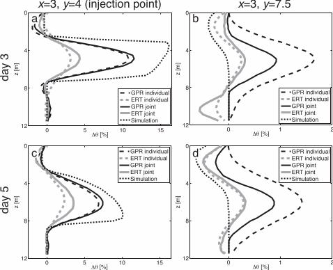
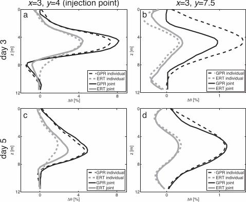
The water content was calculated from the resulting models using equations (6) and (7)
with the petrophysical parameters mentioned above. Vertical profiles of the inferred time-lapse
change in moisture content, , from the background model are shown in Figure 1. It is seen that
the magnitude of is rather well estimated in the GPR inversion but markedly underestimated
in the ERT inversion for both the individual and joint inversions, which can be explained by the
more significant resolution limitations of ERT inversions [Day-Lewis et al., 2005].
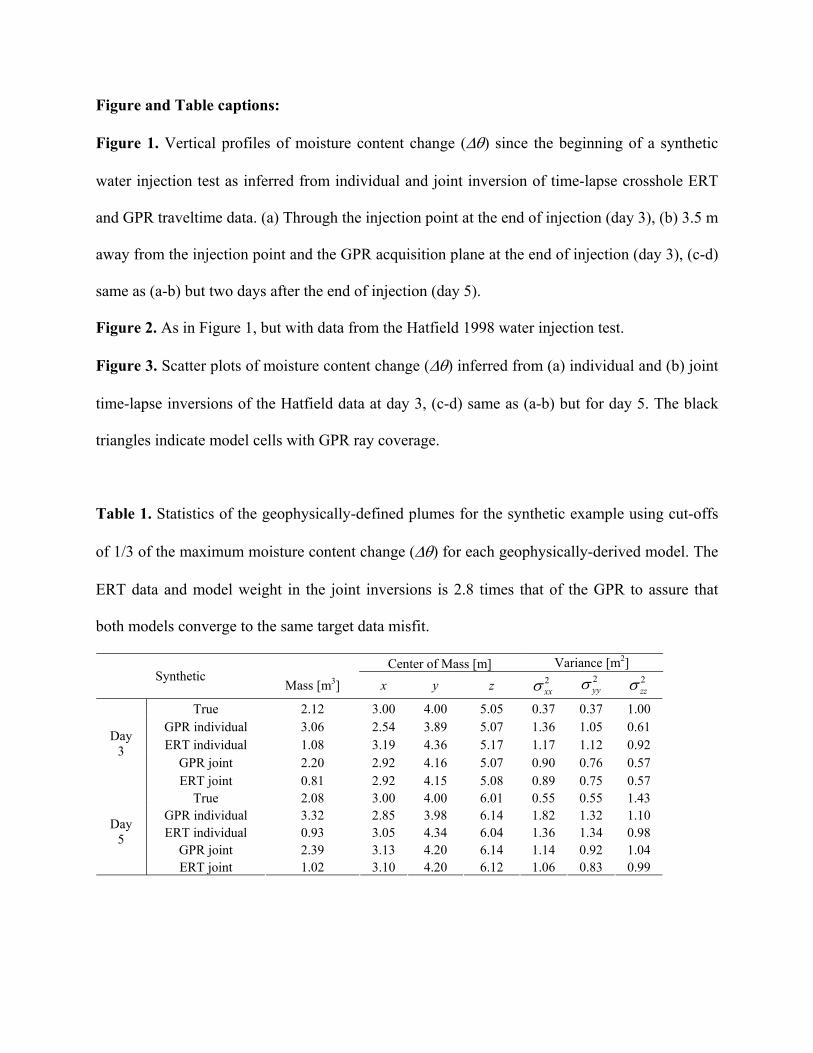
To quantify the changes we define a plume boundary, for each model, at 1/3 of the
maximum . These plumes were then used to calculate the mass, center of mass and the
variances of the plumes, with the resulting statistics presented in Table 1. This plume definition
is rather simplistic [c.f., Day-Lewis et al., 2007], but the relative differences between the
individual and joint inversions are similar for other cut-off values, and serves here only to
investigate if the plume definition is improved by the joint inversion. Note that the 3-D shape of
the plume is heavily dependent on the regularization used as the data sets are acquired between
pairs of boreholes.
The individual GPR inversion model overestimates the mass (+46% (+58%) for day 3 (day
5)), whereas it is more reasonable for the joint inversions (+5% (+13%) for day 3 (day 5)). These
results indicate that the ERT data helps to constrain the geometry of the GPR model that
otherwise is only based on data acquired along one plane and extended in 3-D based on the
regularization. The individual (-49% (-56%) for day 3 (day 5)) and joint ERT (-61% (-51%) for
day 3 (day 5)) models significantly underestimate the mass with no improvement for the joint
inversions.
The error in the center of mass from the individual GPR (0.47 m (0.20 m) for day 3 (day
5)) and ERT inversions (0.42 m (0.34 m) for day 3 (day 5)) are improved in the joint inversion
(0.18 m and 0.17 m, respectively) for day 3, but less so for day 5 (0.20 m and 0.25 m,
respectively). The horizontal variances of the estimated GPR and ERT plumes from the joint
inversions are less overestimated (+100 % on average) than for the individual inversions (+190
% on average). This is due to resolution improvements of joint inversions of crosshole data that
are the most important in the horizontal direction [Linde et al., 2008].
3.3. Hatfield 1998 water injection
Our time-lapse inversion methodology was then applied to the Hatfield field data. Radar
transmission data were acquired using Sensors and Software’s Pulse EKKO radar system with
100 MHz antennas. ERT measurements were acquired using the DMT Resecs resistivity
instrument. The background data sets were inverted individually in 3-D and the final models (not
shown) are consistent with the known geology and fit the data to the specified error levels (see
previous section). The time-lapse data were inverted both individually and jointly in 3-D for 12
iterations such that all inversion results fit the prescribed error level.
Figure 2 shows vertical profiles of the inferred using equations (6) and (7) with the
specified parameter values. These results are consistent with the synthetic example in that the
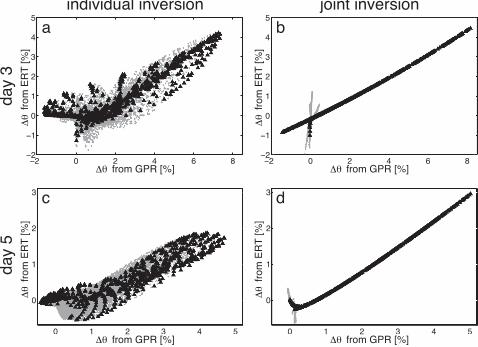
joint inversion models are more focused. Scatter plots of the inversion results show that the
scatter observed in the individual inversions (Figures 3a and 3c) is much reduced and that the
magnitudes are increased in the joint inversions (Figures 3b and 3d). The plumes defined by the
fractional thresholding procedure were then used to calculate the center of mass and the
variances of the plumes (see Table 2). The individual GPR inversion model overestimates the
injected mass of 2100 l (+39% (+57%) for day 3 (day 5)), whereas it is more reasonable for the
joint inversions (+4% (+37%) for day 3 (day 5)). The individual (-50% (-53%) for day 3 (day 5))
and joint ERT (-56% (-54%) for day 3 (day 5)) models both underestimate the mass with no
improvement for the joint inversions.
The differences in the center of mass between the individual GPR and ERT models (0.35
m (0.34 m) for day 3 (day 5)) are improved for the joint inversion at both time-steps (0.05 m
(0.18 m) for day 3 (day 5)). The variance estimates of the GPR and ERT plumes are smaller in
the horizontal direction for the joint compared to the individual inversions (24% on average)
indicating that the joint inversion improves resolution.
4. Concluding remarks
A synthetic experiment based on flow simulations together with field data from a water
injection experiment in unsaturated sandstone show clearly that cross-gradients joint inversion of
crosshole time-lapse ERT and GPR traveltime data decrease horizontal smearing of plumes, that
they increase the similarity between models, and the estimated center of mass of plumes
compared to individual time-lapse inversions. The examples also illustrate that higher resolution
2-D traveltime GPR data might benefit from lower resolution 3-D ERT data. We emphasize that
the inversion methodology presented here is only valid when one state variable varies at each
location of the model domain. For example, if the fluid salinity of the tracer was different to the
native pore water salinity then the resistivity would be a function of moisture content and
salinity, which would violate the assumptions of structural similarity underlying the cross-
gradient constraints.
Acknowledgements
The field data were acquired by P. Winship and R. Middleton, formerly of Lancaster
University. We thank T. Günther, A. Tryggvason and collaborators for providing the ERT and
traveltime forward solvers. A. Binley is grateful to A. Green at ETHZ for generous support that
enabled his contribution. We thank Frederick Day-Lewis and Luis Gallardo for their reviews.
Funding was provided by the Swiss National Science Foundation.
References
Archie, G. E. (1942), The electrical resistivity log as an aid in determining some reservoir
characteristics, Tech. Rep. 1422, Am. Inst. Min. Metall. Pet. Eng., New York.
Binley, A., G. Cassiani, R. Middleton, and P. Winship (2002a), Vadose zone flow model
parameterisation using cross-borehole radar and resistivity imaging, J. Hydrol., 267, 147-159,
doi:10.1016/S0022-1694(02)00146-4.
Binley, A., P. Winship, L. J. West, M. Pokar, and R. Middleton (2002b), Seasonal variation of
moisture content in unsaturated sandstone inferred from borehole radar and resistivity
profiles, J. Hydrol., 267, 160-172, doi:10.1016/S0022-1694(02)00147-6.
Birchak, J. R., C. G., Gardner, J. E. Hipp, and J. M. Victor (1974), High dielectric constant
microwave probes for sensing soil moisture, Proceedings of the IEEE, 62, 93-98.
Day-Lewis, F. D., K. Singha, and A. M. Binley (2005), Applying petrophysical models to radar
travel time and electrical resistivity tomograms: Resolution dependent limitations, J.