+ All Categories
Home > Documents > Structural multi-mechanism model with anisotropic damage ...

Structural multi-mechanism model with anisotropic damage ...

Date post: 23-Mar-2022
Category:
Upload: others
View: 7 times
Download: 0 times
Share this document with a friend
117
STRUCTURAL MULTI-MECHANISM MODEL WITH ANISOTROPIC DAMAGE FOR CEREBRAL ARTERIAL TISSUES AND ITS FINITE ELEMENT MODELING by Dalong Li B.E., Xi’an Jiaotong University, 1998 M.S., Shanghai Jiaotong University, 2003 Submitted to the Graduate Faculty of the Swanson School of Engineering in partial fulfillment of the requirements for the degree of Doctor of Philosophy University of Pittsburgh 2009
Transcript

STRUCTURAL MULTI-MECHANISM MODEL

WITH ANISOTROPIC DAMAGE FOR CEREBRAL

ARTERIAL TISSUES AND ITS FINITE ELEMENT

MODELING

by

Dalong Li

B.E., Xi’an Jiaotong University, 1998

M.S., Shanghai Jiaotong University, 2003

Submitted to the Graduate Faculty of

the Swanson School of Engineering in partial fulfillment

of the requirements for the degree of

Doctor of Philosophy

University of Pittsburgh

2009

UNIVERSITY OF PITTSBURGH

SWANSON SCHOOL OF ENGINEERING

This dissertation was presented

by

Dalong Li

It was defended on

November 13th 2009

and approved by

Anne M. Robertson, Associate Professor, Mechanical Engineering Dept.

William S. Slaughter, Associate Professor, Mechanical Engineering Dept.

Patrick Smolinski, Associate Professor, Mechanical Engineering Dept.

David A. Vorp, Professor, Surgery and Bioengineering Dept.

Dissertation Director: Anne M. Robertson, Associate Professor, Mechanical Engineering

Dept.

ii

Copyright c© by Dalong Li

2009

iii

STRUCTURAL MULTI-MECHANISM MODEL WITH ANISOTROPIC

DAMAGE FOR CEREBRAL ARTERIAL TISSUES AND ITS FINITE

ELEMENT MODELING

Dalong Li, PhD

University of Pittsburgh, 2009

A structural multi-mechanism constitutive equation is proposed to describe the anisotropic

and damage behavior of cerebral arterial tissue. The arterial tissue is modeled as a non-

linear, incompressible and inelastic material. In this model, new deformation criteria are

proposed for the recruitment of collagen fibers and degradation of internal elastic lamina

(IEL), two important features of early stage aneurysm formation.

This structural anisotropic model is formulated by modifying a previous multi-mechanism

model to include the fibrous nature of collagen fibers and incorporates morphological infor-

mation such as fiber orientation and dispersion. An anisotropic damage model is included

to characterize tissue weakening and softening before failure of the IEL, ground matrix or

collagen fibers. Two possible damage mechanisms are formulated in this model: mechani-

cal damage dependent on material strains and enzymatic damage induced by hemodynamic

stresses.

The elastin/ground matrix and collagen fibers are treated as separate components of ar-

teries. The elastin and ground matrix, which are represented by an isotropic response, bear

loads at low strain level, and degrade gradually due to damage or disrupt due to eventual

failure. The collagen fibers are recruited into load-bearing and subfailure damage at higher

strain levels. Two approaches are considered for modeling their anisotropic behavior. In

the first, they are characterized by the anisotropic behavior of N fibers. In the second, the

collagen fibers are arranged in two helically oriented families with dispersion in their orien-

iv

tation. The fiber distribution is modeled by an orientation density function or distribution

parameter. The fiber orientation and dispersion can be prescribed from arterial histology

studies, or identified from stress-strain response as structural parameters.

Pressure inflation test data for cerebral arteries are used to evaluate the constitutive

model. It is found to fit the mechanical response of uniaxial test well. There is a need for

additional experimental data to further evaluate and develop this model. The constitutive

model is implemented in commercial finite element analysis package for numerical compu-

tation. The numerical implementation is validated by analytical solutions. The numerical

model is used for the study of arterial microstructural behavior in complex biomechanical

procedure of angioplasty surgery.

v

TABLE OF CONTENTS

PREFACE . . . . . . . . . . . . . . . . . . . . . . . . . . . . . . . . . . . . . . . . . ix

1.0 INTRODUCTION . . . . . . . . . . . . . . . . . . . . . . . . . . . . . . . . . 1

1.1 Motivation . . . . . . . . . . . . . . . . . . . . . . . . . . . . . . . . . . . . 1

1.2 Cerebral arteries and intracranial cerebral aneurysms . . . . . . . . . . . . . 1

1.3 Histology of cerebral arterial tissues and aneurysms . . . . . . . . . . . . . . 2

1.4 Mechanical behavior of cerebral arterial and aneurysm tissues . . . . . . . . 4

1.5 Model for cerebral aneurysm formation . . . . . . . . . . . . . . . . . . . . . 5

2.0 A STRUCTURAL MULTI-MECHANISM MODEL FOR CEREBRAL

ARTERIES . . . . . . . . . . . . . . . . . . . . . . . . . . . . . . . . . . . . . 7

2.1 Introduction . . . . . . . . . . . . . . . . . . . . . . . . . . . . . . . . . . . 7

2.2 Structural multi-mechanism model for cerebral arterial tissue . . . . . . . . 8

2.2.1 Qualitative features of the multi-mechanism model in cylindrical inflation 8

2.2.2 Elastic mechanical response of elastin and surrounding matrix . . . . 12

2.2.2.1 Deactivation criterion for elastin . . . . . . . . . . . . . . . . . 13

2.2.3 Mechanical response of multi-mechanism material with collagen mech-

anism composed of N fiber families . . . . . . . . . . . . . . . . . . . . 14

2.2.3.1 Constitutive response of N collagen fiber families . . . . . . . 14

2.2.3.2 Activation criterion for recruitment of N-fiber families . . . . . 17

2.2.3.3 Total constitutive response for structural, multi-mechanism model

with collagen mechanism composed of N fiber families . . . . . 18

2.2.4 Mechanical response of multi-mechanism material with distribution

model for collagen fibers . . . . . . . . . . . . . . . . . . . . . . . . . 19

vi

2.2.4.1 Distribution model for collagen fibers . . . . . . . . . . . . . . 19

2.2.4.2 Activation criterion for recruitment of collagen fibers in distri-

bution model . . . . . . . . . . . . . . . . . . . . . . . . . . . 22

2.2.4.3 Total constitutive response for structural, multi-mechanism model

with collagen mechanism composed of a distribution of fibers . 23

2.3 Application of the structural multi-mechanism model to cylindrical inflation 24

2.3.1 Analytic solution for inflation of a cylindrical membrane composed of

the structural multi-mechanism material . . . . . . . . . . . . . . . . . 25

2.3.2 Application of structural multi-mechanism model to the data of Scott,

Fergusen and Roach . . . . . . . . . . . . . . . . . . . . . . . . . . . . 27

2.3.2.1 Results of nonlinear regression analysis . . . . . . . . . . . . . 29

3.0 A DAMAGE MODEL FOR CEREBRAL ARTERIES . . . . . . . . . . 32

3.1 Introduction . . . . . . . . . . . . . . . . . . . . . . . . . . . . . . . . . . . 32

3.2 Damage model for cerebral arteries . . . . . . . . . . . . . . . . . . . . . . . 35

3.2.1 Background for damage models . . . . . . . . . . . . . . . . . . . . . . 35

3.2.1.1 Clausius-Duhem inequality . . . . . . . . . . . . . . . . . . . . 35

3.2.1.2 Clausius-Planck inequality . . . . . . . . . . . . . . . . . . . . 36

3.2.2 Continuum damage models for multi-mechanism materials . . . . . . . 36

3.2.3 Isotropic damage model for the elastin mechanism . . . . . . . . . . . 38

3.2.4 Anisotropic damage model for collagen fibers . . . . . . . . . . . . . . 41

4.0 FINITE ELEMENT IMPLEMENTATION . . . . . . . . . . . . . . . . . . 44

4.1 Numerical scheme . . . . . . . . . . . . . . . . . . . . . . . . . . . . . . . . 44

4.1.1 Slightly compressible structural multi-mechanism model . . . . . . . . 45

4.1.2 Elasticity tensor . . . . . . . . . . . . . . . . . . . . . . . . . . . . . . 48

4.1.3 Elastodamage modulus . . . . . . . . . . . . . . . . . . . . . . . . . . 51

4.2 Numerical validation . . . . . . . . . . . . . . . . . . . . . . . . . . . . . . . 52

4.2.1 Constitutive model for numerical implementation . . . . . . . . . . . . 52

4.2.2 Uniaxial tension tests of one-element . . . . . . . . . . . . . . . . . . . 54

4.2.3 Cylindrical inflation and tension of a thick-walled artery . . . . . . . . 56

4.2.3.1 Kinematics and constitutive response . . . . . . . . . . . . . . 61

vii

4.2.3.2 Analytical solution for pressure and axial force . . . . . . . . . 63

4.2.3.3 Comparison of numerical and analytical solutions . . . . . . . 64

5.0 MODELING OF CEREBRAL ANGIOPLASTY . . . . . . . . . . . . . . 75

5.1 Introduction . . . . . . . . . . . . . . . . . . . . . . . . . . . . . . . . . . . 75

5.2 Finite element model of cerebral angioplasty . . . . . . . . . . . . . . . . . . 77

5.2.1 High pressure response of a multi-layer arterial model . . . . . . . . . 77

5.2.2 Simulation of balloon-artery interaction during cerebral angioplasty . 80

6.0 CONCLUSIONS AND DISCUSSIONS . . . . . . . . . . . . . . . . . . . . 88

BIBLIOGRAPHY . . . . . . . . . . . . . . . . . . . . . . . . . . . . . . . . . . . . 93

viii

LIST OF TABLES

1 Strain energy functions considered for the elastin and collagen mechanisms. . 28

2 Results of nonlinear regression analysis for three choices of strain energy function

for elastin mechanism. . . . . . . . . . . . . . . . . . . . . . . . . . . . . . . . 29

3 Results of regression analysis for 2-fiber, dispersion and isotropic collagen models. 31

4 Representative forms of the constitutive functions implemented in numerical

validation studies. . . . . . . . . . . . . . . . . . . . . . . . . . . . . . . . . . 53

5 Material parameters for an isotropic elastin mechanism (E-EXP1), dispersive anisotropic

collagen mechanism (C-EXP2-disp), volumetric function (VOL) and damage func-

tions (E-DC, E-DF1, E-DF2, E-DF3, C-AC and C-DF), as shown in Table 4. . . . 55

6 Geometry and material parameters of the validation models, with combinations of

first order exponential (E-EXP1) strain energy function for the elastin mechanism,

second order exponential function for the collagen mechanism (C-EXP2-disp), elastin

deactivation criterion (E-DC) and collagen activation criterion (C-AC). . . . . . . 65

7 Geometric and material parameters of the validation models, with a first order ex-

ponential (E-EXP1) strain energy function for the elastin mechanism, second order

exponential function for the collagen mechanism (C-EXP2-disp), Neo-Hookean func-

tion (G-NH)for ground substance, elastin damage criterion (E-DF1) and collagen

activation criterion (C-DF). . . . . . . . . . . . . . . . . . . . . . . . . . . . . . 70

8 Representative forms of the constitutive functions used in angioplasty simula-

tions. . . . . . . . . . . . . . . . . . . . . . . . . . . . . . . . . . . . . . . . . 79

9 Material parameters for three arterial layers in high-pressure response. . . . . . . . 80

10 Material parameters for three arterial layers in balloon-artery interaction. . . . . . 83

ix

LIST OF FIGURES

1 Muscular arterial wall. . . . . . . . . . . . . . . . . . . . . . . . . . . . . . . . 3

2 Components of cerebral arterial and aneurysm walls. . . . . . . . . . . . . . . 4

3 Tension-radius data of an anterior cerebral artery (Scott et al., 1972). . . . . 5

4 Schematic of stages during inflation of a cylindrical membrane composed of

the transversely isotropic, multi-mechanism model. Stage A: Stress-free tissue,

Stage B: Only elastin load bearing, Stage C: Initiation of collagen load bearing,

Stage D: Elastin and collagen load bearing, Stage E: Elastin disruption, Stage

F: Only collagen load bearing, Stage G: Partial disruption of collagen. . . . . 9

5 Schematic of the collagen fiber structure in the arterial wall in the unloaded

configuration. . . . . . . . . . . . . . . . . . . . . . . . . . . . . . . . . . . . 11

6 Schematic of reference configurations for the dual mechanism constitutive model

with relevant kinematic variables drawn. . . . . . . . . . . . . . . . . . . . . . 13

7 Schematic of geometric variables used in dispersion model for collagen fiber

distribution . . . . . . . . . . . . . . . . . . . . . . . . . . . . . . . . . . . . 20

8 Comparison of Neo-Hookean (NH), first order exponential (E-EXP1) and sec-

ond order exponential (E-EXP2) strain energy functions for the elastin mech-

anism of dual-mechanism model, with second order exponential function (C-

EXP2) used for the collagen mechanism for all cases. . . . . . . . . . . . . . 30

9 Comparison of three choices of the collagen mechanism with an exponential

elastin mechanism (i) 2-fiber model (E-EXP2, C-EXP2-2-fiber),(ii) dispersion

model (E-EXP2, C-EXP2-disp), a(ii) isotropic model (E-EXP1, C-EXP1-iso)

used in Wulandana and Robertson (2005). . . . . . . . . . . . . . . . . . . . 31

x

10 Boundary conditions used in the two validation tests. (a): Arterial tissue

strip with uniaxial loading, (b): Cyclically increasing displacement boundary

condition, (c): Step displacement boundary condition. . . . . . . . . . . . . . 55

11 Comparison of two analytical solutions for elastin failure without damage and

elastin cyclic damage d01. Elastin failure at point B and A, respectively, with

the remaining collagen mechanism following load curve 1. . . . . . . . . . . . 57

12 Comparison of two analytical solutions for elastin cyclic damage d01 and d02.

Elastin failure at point A and C, respectively, with the remaining collagen

mechanism following load curve 1. . . . . . . . . . . . . . . . . . . . . . . . . 57

13 Comparison of two analytical solutions for elastin cyclic damage d01 and elastin

cyclic damage d01 with collagen damage dα. For elastin cyclic damage, elastin

fails at point A with the remaining collagen following load curve 1. For elastin

and collagen cyclic damage, elastin fails at point E; collagen starts to experience

damage at point D and fails at point F. . . . . . . . . . . . . . . . . . . . . . 58

14 Comparison of the analytical and numerical solutions for elastin cyclic damage

d01. Elastin failure at point A with the remaining collagen following load curve

1. . . . . . . . . . . . . . . . . . . . . . . . . . . . . . . . . . . . . . . . . . . 58

15 Comparison of the analytical and numerical solutions for elastin cyclic damage

d02. Elastin failure at point C. . . . . . . . . . . . . . . . . . . . . . . . . . . 59

16 Comparison of the analytical and numerical solutions for elastin enzymatic

damage d03 for different choices of WSS and/or WSSG. As these quantities are

increased, the elastin degradation occurs more rapidly. The remaining collagen

following load curve 2 after elastin failure. . . . . . . . . . . . . . . . . . . . . 59

17 Comparison of the analytical and numerical solutions for elastin cyclic dam-

age d01 with collagen damage dα. Elastin fails at point E; collagen starts to

experience damage at point D and fails at point F. . . . . . . . . . . . . . . . 60

18 Cylinder in unloaded configuration κ0 and loaded configuration κ(t). . . . . . 60

19 Symmetric finite element model for the inflation and tension of cylinder. . . . 64

20 Analytical solution for biaxial inflation-tension of 200 µm thick cylinder for

two values of circumferential stretch: (a) λΘi = 3.0 and (b) λΘi = 3.6. . . . . 66

xi

21 Comparison of analytical solution and numerical solution for biaxial inflation-

tension of 200 µm thick cylinder with λΘi = 3.0 and λZ = 1.2. Study of mesh

density. . . . . . . . . . . . . . . . . . . . . . . . . . . . . . . . . . . . . . . . 66

22 Comparison of analytical solution and numerical solution for biaxial inflation-

tension of 200 µm thick cylinder with λΘi = 3.0 and λZ = 1.2. Study of

incompressiblity. . . . . . . . . . . . . . . . . . . . . . . . . . . . . . . . . . . 67

23 Comparison of analytical solution and numerical solution for biaxial inflation-

tension of 200 µm thick cylinder with λΘi = 3.6 and λZ = 1.2. . . . . . . . . . 68

24 Collagen fiber recruitment status for biaxial inflation-tension of 200 µm thick

cylinder with circumferential stretch λΘi = 3.0 and axial stretch λZ = 1.2. . . 68

25 Elastin degradation status for biaxial inflation-tension. . . . . . . . . . . . . . 69

26 Mean orientation of collagen fiber family for biaxial inflation-tension. . . . . . 69

27 Cauchy stress in radial direction for biaxial inflation-tension. . . . . . . . . . 70

28 Comparison of analytical and numerical solutions for cyclic biaxial inflation-

tension of a 200 µm thick cylinder with maximum stretches of λΘi = 2.5 and

λZ = 1.2 for elastin cyclic damage d01. All elastin fails after point G with

collagen left following load curve 3. . . . . . . . . . . . . . . . . . . . . . . . . 71

29 Comparison of analytical and numerical solutions for cyclic biaxial inflation-

tension of a 200 µm thick cylinder with maximum stretches of λΘi = 3.0 and

λZ = 1.2. Elastin cyclic damage d01 with collagen damage dα. All elastin

fails after point H, with collagen and ground substance loaded to point I. All

collagen crimped after point J with ground substance left. . . . . . . . . . . . 72

30 Elastin damage status (d01) for cyclic biaxial inflation-tension of 200 µm thick

cylinder with circumferential stretch λΘi = 3.0 and axial stretch λZ = 1.2. . . 74

31 Collagen fiber damage status (dα) for cyclic biaxial inflation-tension. . . . . . 74

32 Cylindrical multi-layer artery model for biaxial inflation-tension. . . . . . . . 78

33 High pressure response of the multi-layer artery model for biaxial inflation-

tension with axial stretch λZ = 1.1 and internal pressure increased from 0 to

1 bar (State B), then unloaded to 0. . . . . . . . . . . . . . . . . . . . . . . . 81

xii

34 Circumferential Cauchy stress distribution across the deformed wall thickness

at State A. . . . . . . . . . . . . . . . . . . . . . . . . . . . . . . . . . . . . . 81

35 Circumferential Cauchy stress distribution across the deformed wall thickness

at State B. . . . . . . . . . . . . . . . . . . . . . . . . . . . . . . . . . . . . . 82

36 Circumferential Cauchy stress distribution across the deformed wall thickness

at State C. . . . . . . . . . . . . . . . . . . . . . . . . . . . . . . . . . . . . . 82

37 Balloon and artery model for cerebral angioplasty simulation. . . . . . . . . . 83

38 Deformation states of artery and balloon during multi-step cerebral angioplasty

simulation. State A: arterial physiological state before angioplasty (transmural

pressure pi = 13.33KPa and axial stretch λZ = 1.1); State B: initial contact of

the balloon with the artery after balloon deploys; State C: maximum balloon

inflation, arterial dilatation to 130% of its internal diameter; State D: arterial

physiological state after angioplasty, balloon deflation with luminal increase left. 84

39 Damage distribution in the arterial layers at 120% oversized dilation state. The

arrows indicate the locations of the maximum damage: (a) maximum elastin

damage in the IEL d01E = 0.27; (b) maximum ground matrix damage in the

media d01M = 0.21; (c) maximum collagen damage in the media dαM = 0.16. . 85

40 Damage distribution in the arterial layers at 130% oversized dilation state. The

arrows indicate the locations of the maximum damage: (a) maximum elastin

damage in the IEL d01E = 0.83; (b) maximum ground matrix damage in the

media d01M = 0.49; (c) maximum collagen damage in the media dαM = 0.25. . 85

41 Distribution of the circumferential Cauchy stresses in the IEL, media and ad-

ventitia layers at 120% oversized dilation state. The arrows indicate the loca-

tions of the maximum values. . . . . . . . . . . . . . . . . . . . . . . . . . . . 86

42 Distribution of the von Mises stresses in the IEL, media and adventitia layers

at 120% oversized dilation state. The arrows indicate the locations of the

maximum values. . . . . . . . . . . . . . . . . . . . . . . . . . . . . . . . . . 86

43 Distribution of the axial Cauchy stresses in the IEL, media and adventitia

layers at 120% oversized dilation state. The arrows indicate the locations of

the maximum values. . . . . . . . . . . . . . . . . . . . . . . . . . . . . . . . 87

xiii

44 Distribution of the radial Cauchy stresses in the IEL, media and adventitia

layers at 120% oversized dilation state. The arrows indicate the locations of

the maximum values or negative stresses. . . . . . . . . . . . . . . . . . . . . 87

xiv

PREFACE

I would like to thank my advisor, Dr. Anne M. Robertson, sincerely for her guidance and

supervision. Her constant encouragement has been a driving force in the course of my Ph.D.

study and this research work. I would like to express my appreciation to Dr. William S.

Slaughter, Dr. Patrick Smolinski, and Dr. David A. Vorp for serving on my dissertation

committee and their invaluable suggestions and comments. I want to thank Dr. Michael R.

Lovell, Dr. Guoyu Lin and Dr. Sergey Sidorov for the discussion over their research work.

I am very thankful to the Department of Mechanical Engineering and Materials Science

for supporting me with teaching scholarship over the past four years. I also thank ANSYS

Inc. for providing development internship as part of my professional training.

I must thank my colleague students in our research group: Dr. Rachmadian Wulandana,

Michael Hill, Christen Hydrean, Zijing Zeng, Michael Durka, Hasballah Zakaria and Mahzad

Bastani Nejad for spending time together in the valuable discussions and collaborations.

I would like to sincerely thank Glinda Harvey and Brittany Guthrie for providing crucial

administration and help essential to my studies and work.

I am indebted and grateful to my family. My deeply thanks to my father Yingtian Li,

my mother Yanling Yu, and my sisters Xiaohong Li and Xiaojun Li for their love, support,

and encouragement. My sincere thanks to my wife Jenny Yue Cui, also my best friend, for

exploring the world with me, and for giving me a handsome son Jonathan Haoyang Li, whose

brilliant smile is always shining our life.

xv

1.0 INTRODUCTION

1.1 MOTIVATION

The motivation of the current work is the study of the biomechanics of the formation of

human intracranial aneurysms. The initiation and development of arterial aneurysms are

complex biological and mechanical processes. At this point in time, most theories regarding

the formation mechanisms are hypotheses, which need further exploration and validation.

Our long-term objective is to understand the biomechanical mechanisms of aneurysms

and vascular injuries. A theoretical approach is taken in this dissertation by developing

constitutive models for arterial walls and robust numerical implementation of these models.

The constitutive models are motivated by current experimental studies, and can be used to

analyze the mechanical response of cerebral arteries. Numerical simulations can help us to

explore the micromechanical behavior of tissue components due to realistic biomechanical

factors.

1.2 CEREBRAL ARTERIES AND INTRACRANIAL CEREBRAL

ANEURYSMS

Intracranial cerebral aneurysms (ICA) are local dilatations of cerebral arterial walls. Most

ICA are saccular and 2 mm or more in diameter. ICA are commonly found at the bifurcation

or curved area of cerebral arteries in or near the Circle of Willis (Camarata et al., 1992),

and often show a clear neck region.

1

Saccular aneurysms are very common in US populations. An angiography study revealed

a 1% incidence of anterior circulation aneurysms in the U.S. general population (Atkinson et

al., 1989). Other autopsy studies reported 0.8-8.1% incidence of saccular aneurysms in the

U.S. population (McCormick and Acosta-Rua , 1970; Inagawa and Hirano, 1990).

Rupture of cerebral aneurysms is very dangerous for the patient. When aneurysms rup-

ture, the blood will flood into the subarachnoid space and cause a subarachnoid hemorrhage

(SAH). The highest reported incidence of ruptured aneurysms in autopsy studies is 3% among

the population of the United States (McCormick and Acosta-Rua , 1970). The incidence of

patient death following aneurysm rupture is over 50% (Ingall et al., 1989; Broderick et al.,

1994), while 14-20% of the patients are disabled moderately or severely (Broderick et al.,

1994; Longstreth et al., 1993).

1.3 HISTOLOGY OF CEREBRAL ARTERIAL TISSUES AND

ANEURYSMS

Cerebral arteries are muscular arteries with a distinct three-layer structure: the intima, media

and adventitia (Rhodin, 1979), Fig. 1. The intima is the innermost layer of the artery, and is

composed of a single layer of endothelial cells resting on a thin basal membrane. In a healthy

young person, the intima is usually very thin and ignored for the mechanical properties of

the artery. The media is in the middle of the artery, and primarily consists of smooth muscle

cells and collagen fibrils between them. The adventitia is the most outer layer of the artery.

It consists mainly of thick bundles of collagen fibers plus ground substances (Rhodin, 1979;

Stehbens et al., 1972). In typical muscular arteries, the media is separated from the intima

and adventitia by an internal elastic lamina (IEL) and external elastin lamina (EEL), both

composed of fenestrated sheets of elastin (Stehbens et al., 1972). Cerebral arteries have a

thicker IEL, thinner media and no EEL compared with other arteries. Elastin and collagen

fibers are the two significant contributors to the passive mechanical properties of arteries.

The elastin of cerebral arteries is concentrated in the IEL but more broadly distributed

2

throughout the arterial wall in extracranial arteries. Histological studies of human arteries

have shown the collagen fibers are in a wavy state in unloaded arteries and progressively

straighten with loading (Samila and Carter, 1981).

The arterial tissue of cerebral aneurysm walls is structurally different from healthy ar-

teries, Fig. 2. At the orifice of the sack, the media terminates, and the IEL is fragmented, or

slightly extends into the aneurysm neck region. In the aneurysm wall away from the orifice,

the media is completely absent and the IEL is totally disrupted (Crawford, 1959; Cajander

and Hassler, 1976).

Adventitia

Media

EEL

Endothelium

IEL

Figure 1: Muscular arterial wall.

The three-dimensional organization of collagen fibers and muscle cells in cerebral arteries

has been investigated experimentally. Peters et al. (1983) showed that cerebral arteries have

highly oriented medial muscle cells, aligned circumferentially with very small variation in

angle. Finlay et al. (1995) found that collagen and smooth muscle cells in the media are con-

sistently circumferentially and coherently aligned, while the collagen fibers in the adventitia

are highly varied in coherence and mean direction with a substantial component of longi-

tudinal fibers. At increasing pressures, the collagen fibers in all layers become increasingly

coherent and more circumferential in direction (Finlay et al., 1995).

3

Adventitia

Endothelium

Endothelium

fundus

orifice

Media

IEL

Cerebral artery walls Bleb/cerebral aneurysm walls

Figure 2: Components of cerebral arterial and aneurysm walls.

1.4 MECHANICAL BEHAVIOR OF CEREBRAL ARTERIAL AND

ANEURYSM TISSUES

The mechanical properties of cerebral arteries is very important for the understanding of

tissue behavior in aneurysm initiation, development and rupture, which are complex biome-

chanical processes. In-vitro and in-vivo tests of human cerebral arterial tissue is still a

challenging task. To date, there is still limited experimental data available for the nonlinear

and inelastic response of cerebral arteries to test hypotheses on aneurysm etiology. Monson

(2001) studied the failure properties of human cerebral arteries, and reported the uniaxial

and biaxial mechanical response (Monson et al., 2003, 2006).

In their pioneering work, Scott et al. (1972) explored the hypothesis that the main differ-

ence in mechanical properties between cerebral arterial and aneurysm tissue is due to elastin

degradation during the aneurysm formation process. As part of their work, they inflated seg-

ments of cerebral arterial tissue in-vitro to obtain pressure-volume data. Significantly, they

found that after three runs to 200 mmHg, the mechanical properties of the tissue changed

abruptly and the unloaded radius of the vessel increased, Fig. 3.

The tension-stretch curve for the later loading cycles had no toe region, but was repeat-

able. Scott et al. (1972) found similar results for all three cerebral arteries loaded to this

level. No shift was seen in control experiments of cyclic loading to a maximum pressure of

4

100 mm Hg. They hypothesized the qualitative change in the curve was due to the disrup-

tion of the elastin membrane caused by mechanical loading beyond the breaking strength

of elastin. Their conjecture was based on (i) the lack of toe region in the second runs, and

(ii) the qualitative similarity in the curves for the second runs and those of arterial tissue in

which elastin had been chemically removed as a load bearing component (Roach & Burton,

1957). This is also consistent with the histological study (Nystrom et al., 1963) showing that

the aneurysm tissue has decreased and fragmented elastin.

Figure 3: Tension-radius data of an anterior cerebral artery (Scott et al., 1972).

1.5 MODEL FOR CEREBRAL ANEURYSM FORMATION

To better understand the mechanisms of aneurysm formation, instead of modeling arteries

and aneurysms as distinct entities with independent reference configurations (Canham and

Ferguson, 1985; Hademenos et al., 1994; Hung and Botwin, 1975; Ryan and Humphrey,

1999), Wulandana and Robertson (2005) developed a multi-mechanism, inelastic constitutive

5

equation to model the initiation and early development stages of cerebral aneurysm from

a segment of arterial wall. In that work, elastin and collagen fibers were modeled as two

distinct mechanisms with different mechanical properties and unloaded configurations. The

recruitment of collagen fibers and degradation of the internal elastic lamina are initiated

based on the deformation state in the arterial wall. To our knowledge, this is the first attempt

at modeling early stage aneurysm formation including these two important characteristics.

Isotropic material responses were used for both elastin and collagen, and exponential strain

energy functions were found to have the best fit with the pressure inflation experimental data

of Scott et al. (1972). While this model is structurally motivated, it is phenomenological in

nature.

6

2.0 A STRUCTURAL MULTI-MECHANISM MODEL FOR CEREBRAL

ARTERIES

2.1 INTRODUCTION

Anisotropic structural constitutive models have been developed for a variety of soft tissues.

Although phenomenological models are successfully used to fit biaxial experimental data,

the material constants do not reflect the structural properties. By comparison, structural

constitutive models integrate more information on tissue composition, structure, and the

load carrying mechanisms of individual parts, so provide more insight into the function and

mechanics of tissue components (Lanir, 1983). A more detailed review of structural models

for arterial tissue can be found in Gasser et al. (2006). The most complete approach has been

presented by Lanir (1983) and Lanir et al. (1996). In his model for fibrous connective tissues,

the total strain energy of tissue is assumed to be the sum of individual fibers, and the fiber

strain is related to the global strain by a tensor transformation between global coordinates

and fiber coordinates. Lanir included fiber orientation in the model through prescribed

statistical distributions and obtained the distribution parameters from experimental data.

Sacks (2000); Billar & Sacks (2000) and Sacks (2003) developed an experimental method

for measuring the distribution of collagen fiber angles in some tissues using small angle

light scattering (SALS) and developed a structural model based on Lanir′s work. This

was the first structural model with parameters derived directly from experimental measures

of fiber orientation. Holzapfel et al. (2000) proposed a fiber-reinforced structural model

for arteries, in which two families of collagen fibers are assumed to be embedded in an

isotropic ground matrix. In accordance with arterial histology, this model seems to represent

the media architecture better than the intima and adventitia architecture (Gasser et al.,

7

2006). Motivated further by the study of arterial tissue morphology (Canham et al., 1989;

Finlay et al., 1995), Gasser et al. (2006) generalized Holzapfel′s model to include a large

range of fiber orientations. They introduced an orientation density function to characterize

collagen fiber distribution with respect to a reference orientation in the unloaded reference

configuration. A scalar structure parameter is obtained from the integration of the density

function and represents the degree of anisotropy. This model was used to describe the

fiber dispersion characteristics of the intima and adventitia in arterial tissue. Lanir′s and

Holzapfel′s structural models have been used successfully in some recent fibrous tissue models

(De Vita and Slaughter, 2006; Natali et al., 2004, 2005; Gasser and Holzapfel, 2002).

In this study, an anisotropic, structural, multi-mechanism constitutive model is developed

to describe the mechanical behavior of cerebral arteries. The material anisotropy arising from

the collagen fiber orientation in cerebral vessels is modeled using the approach of Holzapfel

et al. (2000) and Gasser et al. (2006). The fiber orientation is modeled using two approaches

(i) a finite number of fiber families and (ii) a fiber distribution function. A new parameter

for collagen recruitment based on local collagen stretch is used. Published inelastic pressure

inflation data (Scott et al., 1972) are used to select the specific form of the strain energy

function. There is a pressing need for multi-axial experiments to further refine this model.

2.2 STRUCTURAL MULTI-MECHANISM MODEL FOR CEREBRAL

ARTERIAL TISSUE

2.2.1 Qualitative features of the multi-mechanism model in cylindrical inflation

To elaborate fundamental roles of different mechanisms, we first discuss the qualitative fea-

tures of quasi-static inflation of an arterial segment which is idealized as a transversely

isotropic, multi-mechanism material. Here, the artery wall is idealized as a homogeneous,

single-layer, cylindrical membrane in which case the inflation deformation is also homoge-

neous. In sections 2.2.2, 2.2.3 and 2.2.4, we will discuss the general 3-D case and rigorous

continuum formulation. In order to clarify the separate and changing roles of the elastin

8

and collagen mechanisms during loading, we subdivide the deformation into seven possible

stages, Fig. 4. Cylindrical coordinates (r, θ, z) with z-axis aligned with the artery centerline

and corresponding basis (er, eθ, ez) will be used to discuss the idealized deformation. Elastin

is shown as red color before disruption, and white after disruption. Collagen fibers are shown

as black lines.

Stage F

Rb<R<Rc

Stage E

R=Rb

κb

Stage G

R=Rc

κc

Stage B

R0<R<Ra

R

Collagen

fibersStage A

R=R0

Stage C

R=Ra

Stage D

Ra<R<Rb

Elastin

κ0

κa

Figure 4: Schematic of stages during inflation of a cylindrical membrane composed of the

transversely isotropic, multi-mechanism model. Stage A: Stress-free tissue, Stage B: Only

elastin load bearing, Stage C: Initiation of collagen load bearing, Stage D: Elastin and

collagen load bearing, Stage E: Elastin disruption, Stage F: Only collagen load bearing,

Stage G: Partial disruption of collagen.

Stage A denotes the stress-free configuration, κo of the cylindrical membrane with surface

R = R0. This is also the unloaded configuration. Motivated by the morphology of arteries

(Rhodin, 1979; Stehbens et al., 1972), we extend the model of Wulandana and Robertson

(2005) and treat the unloaded state as composed of separate mechanisms: an isotropic mech-

9

anism largely controlled by the response of elastin and the surrounding matrix as well as

an anisotropic response arising from a helical network of crimped collagen fibers. These

crimped fibers require a finite deformation to bear load. The contribution of fibers in the

radial direction are neglected but can be included if their inclusion is supported by experi-

mental data. By way of illustration, in this section we consider one pair of fibers with angles

β1 = β, β2 = −β, without dispersion in the plane of the membrane, Fig 5.

As the artery is pressurized, the lateral surface of the membrane moves to radial posi-

tion R. During Stage B, the deformation is sufficiently small that the collagen fibers show

diminishing waviness and change their orientation without contributing significantly to load

bearing. The stress generation is dominated by elastin, corresponding to the toe region in

a typical stress/stretch curve (Busby and Burton, 1965). In further discussions, we denote

the circumferential stretch of the membrane as λ. For example, during Stage B, λ = R/R0.

In this work, the symmetry of unloaded fiber orientation and symmetric form of the defor-

mation are such that the two families of fibers undergo the same fiber stretch for all times,

which we denote as λf . The subscript f is used to emphasize that, in general, the fiber and

circumferential stretch are different.

At Stage C, a critical level of λf is reached, denoted as λfa when the waviness has dimin-

ished to the point that under further stretch, the fibers will bear load. Hence, the quantity

λfa reflects the degree of waviness of the collagen fibers in the unloaded material. The cor-

responding radius of the artery in this configuration is denoted as Ra, the circumferential

stretch as λ = λa and the configuration as κa. The subscript a is used to emphasize the

activation of the collagen mechanism in this configuration. It follows that λa = Ra/R0. The

fiber stretch λfa can be computed from the tensorial transformation of the global membrane

stretch λa referenced to fiber coordinates, assuming the deformation is affine.

Upon further loading, Stage D, both the collagen and elastin mechanisms contribute

to load bearing. The contribution of the elastin mechanism continues to depend on the

deformation relative to κ0, while the stress within the collagen fibers is a function of the

fiber stretch relative to stretch λfa. The addition of the stiffer collagen fibers leads to the

steep increase in stiffness in the stress/stretch curve in Stage D, ending the shallow toe region

of Stage B (Busby and Burton, 1965; Hoffman et al., 1977; Samila and Carter, 1981).

10

a1,0

a2,0

β1β2

R0

Figure 5: Schematic of the collagen fiber structure in the arterial wall in the unloaded

configuration.

Upon further loading, Stage E, a critical radius is reached Rb where the elastin mecha-

nism is disrupted to the point of ceasing to contribute to load bearing. The corresponding

circumferential stretch of the membrane is denoted as λb = Rb/R0 and the configuration as

κb. In a purely mechanical theory, this disruption is entirely due to an increase in mechanical

loading and the criterion for disruption is purely a function of a kinematic measure of the

deformation. We conjecture that in some cerebral arteries, for example during early stages

of aneurysm formation, this critical level of stretch may be reached even under fixed pres-

sure due to a degradation of the IEL arising from a combination of factors such as fatigue,

extended periods of exposure to elevated hemodynamic loading such as wall shear stress and

wall shear stress gradient (Robertson et al., 2007), damage due to environment factors, and

aging (Busby and Burton, 1965; Samila and Carter, 1981). Disruption of the IEL is a feature

common to all cerebral aneurysm walls and has been hypothesized to be associated with the

inelastic behavior of cerebral arteries and with the initiation of an ICA (Scott et al., 1972).

Upon further loading (or unloading), Stage F, only collagen will contribute to load bear-

ing. Unloading during this stage, will return the fibers to stretch λfa. As a result, the

unloaded radius will increase. If the arterial segment without a functioning IEL is consid-

ered as a second material, it will appear stiffer than the original artery, and will not display

11

a toe region. This behavior of our model is consistent with mechanical data from Scott et

al. (1972) and Roach & Burton (1957).

We expect that an additional stage, Stage G, will be associated with partial collagen

disruption and potentially the generation of new collagen in an altered reference configuration

as part of a longer time scale process, involving growth and remodeling (Wulandana and

Robertson, 2005; Humphrey, 2002).

2.2.2 Elastic mechanical response of elastin and surrounding matrix

This discussion of the kinematics for the elastin mechanism follows that in Wulandana and

Robertson (2005). A section of cerebral artery will be represented by a three-dimensional

body B which initially, say at time t = t1, is stress free and occupies a region that will

be referred to as the undeformed reference configuration κ0. A typical material particle,

labeled Y , in the body B will be identified by vector position X0 in κ0 relative to a chosen

coordinate system, Fig. 6. Using this notation, the motion of an arbitrary material particle

Y can be described through the relationship

x = χκ0(X0, t), (2.1)

where the vector function χκ0(X0, t) is single-valued, invertible and continuously differen-

tiable with respect to its arguments as many times as required in the subsequent analysis.

The configuration at arbitrary time t > t1 will be denoted by κ(t). The deformation gradient

F 0 at time t for an arbitrary material particle Y in reference configuration κ0 is given by

F 0 = F κ0(X0, t) =

∂χκ0(X0, t)

∂X0

. (2.2)

The associated left and right Cauchy Green tensors for κ0 are then,

B0 = F 0 · F T0 , C0 = F T

0 · F 0. (2.3)

As in Wulandana and Robertson (2005), we model the mechanical response of the first mech-

anism using a hyperelastic strain energy function per unit volume in reference configuration

κ0 as ψ0 = ψ0(F 0). Based on invariance requirements and assuming the material is isotropic

12

with respect to configuration κ0, the strain energy function reduces to ψ0 = ψ0(I0, II0) where

I0 and II0 are the first and second invariants of C0,

I0 = I(C0) = tr C0, II0 = II(C0) =1

2

[(tr C0)

2 − tr C20

]. (2.4)

Furthermore, as in Wulandana and Robertson (2005), we will assume the isotropic mech-

F1 . a1,1 F1 . a2,1

κ(t)

κ1

a1,1 a2,1

dX0

x = χκ1(X1, t)

a1,0 a2,0β

X1 = χκ0(X0, t)

dX1

dx

X0

κ0

dx = F0 . dX0= F1 . dX1

Stage A Stage D

Stage E

Figure 6: Schematic of reference configurations for the dual mechanism constitutive model

with relevant kinematic variables drawn.

anism ψ0 is dominated by the dependence on I0 and the effect of II0 is comparatively

negligible.

ψ0 = ψ0(I0). (2.5)

2.2.2.1 Deactivation criterion for elastin As in Wulandana and Robertson (2005),

we assume there exists a critical level of deformation when the first mechanism is disrupted

and ceases to contribute to load bearing. We introduce a metric of loading for the elastin

mechanism, called the deformation state parameter, which is chosen to be a monotonically

increasing function of I0,

s0 = s0(I0). (2.6)

13

Without loss in generality, we choose a linear function,

s0 = max(I0 − 3), (2.7)

normalized so that s0 is zero when there is no deformation. The criterion for deactivation

of the first mechanism will then be defined through a deactivation criterion of the form

s0 = s0b. Once s0 ≥ s0b for some deformation, elastin no longer contributes to load bearing

in all further deformations, even when s0 develops below s0b.

In Section 3.2.3, we will generalize the constitutive response to include progressive dam-

age of this isotropic mechanism. As discussed below, we can extend the functional depen-

dence of ψ0 to include the effect of changes in mechanical response of elastin arising due to

aging, fatigue related factors, and deleterious hemodynamic loads (Robertson et al., 2007).

2.2.3 Mechanical response of multi-mechanism material with collagen mecha-

nism composed of N fiber families

In this section, the fiber orientation is modeled using a finite number of fiber families. The

mechanical model for the contribution of the collagenous fibers builds on that introduced by

Lanir (1983), Lanir et al. (1996) and Holzapfel et al. (e.g. Holzapfel et al., 2000; Holzapfel,

2000, Section 6.7). While in these works, a single zero stress state reference configuration

was employed for all material constituents, here we introduce an additional reference config-

uration κi for each fiber with an associated activation criterion. This additional constitutive

structure makes it possible to capture the change in unloaded configuration when the first

mechanism is disrupted.

2.2.3.1 Constitutive response of N collagen fiber families We assume any anisotropic

response of the material arises from the contribution of collagenous fibers in the wall. At

each point in space, the collagen contribution is represented by N fibers. The direction of an

arbitrary fiber i in κ0 is characterized by a unit vector ai,0 which makes an angle βi relative to

a reference direction in κ0, Fig. 5. The first subscript on a is the fiber number and the second

is the configuration. For example, using eθ as the reference angle, ai,0 = cos βieθ + sin βiez

14

is the direction of fiber i in configuration κ0. We further assume the fibers move affinely

with the underlying material during the deformation. Therefore, an infinitesimal material

element of fiber i, denoted as dX0 = dS0 ai,0 at point X0 in configuration κ0, will be mapped

to dx = F 0 · ai,0 dS0 at x in configuration κ(t), Fig. 6. The stretch of this infinitesimal fiber

material element relative to its length in κ0 is therefore,

λ2i,0 =

|dx|2|dX0|2

= C0 : ai,0 ⊗ ai,0. (2.8)

The unit vector ai,0 represents the direction of fiber i in κ0 is mapped to F 0 · ai,0 in κi. This

new fiber direction can be normalized as a unit vector ai,i,

ai,i =1

λi,0

F 0 · ai,0. (2.9)

In the qualitative discussion in Section 2.2.1, when the fibers reached a critical stretch

λfa, they became load bearing and this critical stretch was fiber independent. More generally,

λfa will be different for different fibers and we will denote the critical stretch for fiber i as

λia and the corresponding configuration as κia,

λ2ia = λ2

i,0|κia, (2.10)

where |κia after a quantity is used to denote that the quantity takes the value it held in

configuration κia.

The mechanical response of collagen fiber i will depend on the stretch beyond λia and

we therefore turn attention to kinematic quantities defined relative κia. The motion of a

particle at time t (configuration κ), which has position X i in configuration κia is,

x = χκia(X i, t), (2.11)

and the corresponding deformation gradient relative to κia is,

F i = F i(X i, t) =∂χκia

(X i, t)

∂X i

. (2.12)

The associated left and right Cauchy Green tensors are,

Bi = F i · F Ti , C i = F T

i · F i i = 1,2,...,N. (2.13)

15

In configuration κ, the deformation gradient F i is related to F 0 (the deformation gradient

relative to κ0) through,

F i = F 0 · F 0−1|κia

, (2.14)

and therefore

Ci = F 0−T |κia

· C0 · F 0−1|κia

. (2.15)

As in Holzapfel et al. (2000), we assume the collagen mechanism can be modeled as the

collective response of N fibers, each of which behaves as a hyperelastic, transversely isotropic

material. The total strain energy function for the collagen mechanism is then,

ψaniso =N∑

i=1

ψi(Ci, ai,i ⊗ ai,i). (2.16)

Note, the form (2.16) implicitly assumes the response of the fibers are decoupled. Since the

material response should not depend on the sign of ai,i, it has been included in the strain

energy function (2.16) as a tensor product,

Ai,i = ai,i ⊗ ai,i, (2.17)

which is sometimes referred to as the structure tensor (Holzapfel et al., 2000; Gasser et al.,

2006).

The integrity basis for the symmetric second order tensors Ci, Ai,i (i=1,2,...,N) is com-

posed of the following invariants (e.g. Holzapfel et al., 2000),

Ii = tr Ci, IIi =1

2

[(tr Ci)

2 − tr C2i

], IIIi = 1,

IVi,i = Ci : Ai,i, Vi,i = C2i : Ai,i.

(2.18)

A strain energy function of the form (2.16) which is transversely isotropic can therefore be

written as (Holzapfel et al., 2000),

ψaniso =N∑

i=1

ψi(Ii, IIi, IVi,i, Vi,i). (2.19)

For lack of extensive data for the anisotropic behavior of cerebral arteries, we reduce the

dependence of ψaniso to the simplest form that is consistent with the expected mechanism

16

of collagen load bearing. In particular, we assume the response of the collagen fibers is

dominated by the stretch of individual collagen fibers relative to the stretch in reference

configuration κia, which is denoted by, λi,i. Noting that an infinitesimal fiber element dXi =

dSi ai,i in configuration κia will be mapped to dx = F i · ai,i dSi in κ, it follows that,

λ2i,i =

|dx|2|dXi|2

= Ci : ai,i ⊗ ai,i = IVi,i. (2.20)

We therefore, simplify Eq. (2.19) to

ψaniso =N∑

i=1

ψi(IVi,i). (2.21)

Note that λi,i is related to λi,0 through,

λi,i =λi,0

λia

. (2.22)

2.2.3.2 Activation criterion for recruitment of N-fiber families We introduced

λia as a material parameter defining the stretch at which fiber i is load bearing. Here, we

restate this condition in terms of kinematic invariants. As in Wulandana and Robertson

(2005), we introduce a deformation state parameter which serves as a metric of the relevant

aspects of the deformation. In that work, the collagen mechanism was modeled as isotropic

and the metric was chosen to be a function of I0. The same metric was used for both collagen

and elastin. Here, we consider the role of collagen fibers and use the collagen stretch λi,0

defined in (2.8) as a measure of this deformation from the strain free state in κ0. We define

the deformation state parameter for collagen as a monotonically increasing scalar function

for fiber i

si = si(IVi,0), (2.23)

where

λ2i,0 = IVi,0 = C0 : ai,0 ⊗ ai,0. (2.24)

As shown in (2.23), the state parameter for the fibers depends only on one variable. Without

loss in generality, we choose a linear function,

si = IVi,0 − 1, (2.25)

17

normalized so that si is zero when the body is unloaded, κ0. Fiber i will be considered

uncrimped when si reaches a critical value, si = sia. Denoting IVia,0 as the corresponding

critical value of the IVi,0,

sia = si(IVia,0). (2.26)

It follows from (2.8) and (2.10) that IVia,0 is related to λia through,

IVia,0 = λia2. (2.27)

In the case of homogeneous deformations, with homogeneous fiber distribution, IVi,0 will

be constant throughout the material and hence the criterion (2.27) will be met simultaneously

at all points in the body. However, more generally, activation of the collagen fiber i can occur

at different times t for different points in the body if, for example, λia takes the same value

throughout the material (material is homogeneous with respect to this parameter), but the

deformation is inhomogeneous. In addition, the activation criterion will be met at different

times at points in the body, if the deformation is homogeneous but the value of λia varies in

the body.

2.2.3.3 Total constitutive response for structural, multi-mechanism model with

collagen mechanism composed of N fiber families At arbitrary time and material

point, the strain energy function of anisotropic cerebral arterial tissue can be expressed as:

ψ = (1− d0)ψ0(I0) +N∑

i=1

(1− di)ψi(IVi,i) (2.28)

where d0 and di are weighting functions for elastin deactivation and collagen activation,

respectively,

d0 =

0 s0 < s0b

1 s0 ≥ s0b,(2.29)

di =

1 si < sia, i ∈ [1, N ]

0 si ≥ sia, i ∈ [1, N ].(2.30)

18

It is assumed that once the elastin mechanism has been deactivated, it cannot be activated

again.

The corresponding Cauchy stress tensor is (Holzapfel, 2000),

T = −pI + 2(1− d0)∂ψ0

∂I0

B0 +N∑

i=1

(1− di)

[2

∂ψi

∂IVi,i

F i · ai,i ⊗ F i · ai,i

](2.31)

2.2.4 Mechanical response of multi-mechanism material with distribution model

for collagen fibers

2.2.4.1 Distribution model for collagen fibers In the previous discussion, the con-

tribution of N fibers are modeled independently. In this section, we simplify the constitutive

equation by replacing the N fiber response with a collective response of dispersed fibers

(Gasser et al., 2006). By way of example, here the artery wall is characterized by two

families of dispersed fibers with mean directions β1, β2 in κ0,

aα,0 = cos βαeθ + sin βαez, α = 1, 2. (2.32)

Furthermore, it is assumed the fibers are distributed with rotational symmetry such that

β1 = −β2. In the arterial model, this symmetry will correspond to transverse isotropy of

the material. It should be emphasized that previously βi represented the direction of fiber i

(i=1,2,...,N). Here, β1, β2 are the mean directions of dispersed families of fibers.

As in Gasser et al. (2006), the three-dimensional distribution of fiber angles is modeled

using an orientation density function ρ(M(Θ, Φ)) which characterizes the three-dimensional

distribution of fiber angles in the reference configuration κ0 with respect to a reference

orientation M , Fig. 7. In the most general case, M is an arbitrary unit vector which is

characterized by two Euler angles Θ ∈ [0, π] and Φ ∈ [0, 2π] in a three-dimensional Cartesian

coordinate system with basis {e1, e2, e3},

M(Θ, Φ) = sin Θ cos Φe1 + sin Θ sin Φe2 + cos Θe3. (2.33)

19

x1

x2

x3

Me3

e2

e1 φ

θ

x1

x2

x3

Me3

e2

e1 φ

θ

Figure 7: Schematic of geometric variables used in dispersion model for collagen fiber distri-

bution

A non-negative density function is defined such that ρ(M(Θ, Φ))dω represents the nor-

malized number of fibers with orientations in the range [(Θ, Θ + dΘ), (Φ, Φ + dΦ)], where

dω = sin ΘdΘdΦ. Furthermore, ρ is symmetric with respect to M and normalized,

ρ(M) = ρ(−M) and1

ω

ρ(M(Θ, Φ)) dω = 1. (2.34)

While the fiber orientation is, in general, characterized by ρ, for the special case of

the artery model where the fibers have rotational symmetry about some mean referential

direction aα,0, it is convenient to characterize this orientation in terms of a generalized

symmetric second order tensor H,

H =1

∫ρ(M(Θ, Φ))M(Θ, Φ)⊗M(Θ, Φ) sin Θ dΘ dΦ, (2.35)

and referred to as the structure tensor, (Gasser et al., 2006), which accounts for the collective

contribution of dispersed fibers in all directions. Choosing Cartesian coordinates, such that

aα,0 is equal to e3, it follows that the density function ρ is independent of Φ. It can then

be shown, (Gasser et al., 2006), that for each family of fibers the structure tensor can be

written with respect to a single dispersion parameter, k, in κ0,

Hα,0 = kI + (1− 3k)aα,0 ⊗ aα,0, (2.36)

20

where I is the identity tensor, and k is defined as a structure parameter that represents the

fiber distribution in an integral sense, describing the degree of anisotropy,

k =1

4

∫ π

0

ρ(Θ) sin3(Θ) dΘ. (2.37)

The parameter k can either be thought of as a material parameter, determined directly from

the experimental data, or calculated, from experimental knowledge of ρ(Θ). When there is

an isotropic distribution of collagen fibers, ρ equals one, so k = 1/3 and the structure tensor

H is proportional to the identity tensor. Furthermore, if ρ is chosen to be proportional to

a Dirac delta function, namely, ρ = Kδ(Θ0) where K is a constant and δ(Θ0) is the Dirac

delta function then for Θ0 ∈ (0, π), k = 1/2sin2(Θ0).

The anisotropic strain energy function for the dispersed collagen mechanism based on

the generalized structure tensor H is,

ψaniso =2∑

α=1

ψα(Cα, Hα,α), (2.38)

which is analogous to Eq. (2.16). Here, Hα,α is the structure tensor of αth fiber family in

its reference configuration κα associated with an activation criterion, and Cα is the right

Cauchy Green tensor defined by the deformation gradient Fα relative to κα,

Cα = F Tα · Fα. (2.39)

We now assume the only anisotropy in the material is due to families of dispersed fibers

and therefore require,

ψα(Cα, Hα,α) = ψα(Q · Cα ·QT , Q ·Hα,α ·QT ), (2.40)

for all proper orthogonal Q. Therefore, without loss in generality, the strain energy for

fiber family i can be written with respect to its integrity basis for (Cα, Hα,α) (Spencer ,

1984). For lack of extensive data for the anisotropic behavior of cerebral arteries, we reduce

the dependence of ψα on these invariants to the simplest form that is consistent with the

expected mechanism of collagen load bearing for incompressible materials.

21

In particular, we assume the response of the collagen fibers is dominated by Eα,α, the

strain in the mean direction of a fiber family relative to κα,

Eα,α = kIα + (1− 3k)IVα,α − 1, (2.41)

so that ψα = ψα(Iα, IVα,α). The anisotropic strain energy function then can be written in

terms of two tensor invariants (Gasser et al., 2006),

ψaniso =2∑

α=1

ψα(Iα, IVα,α), Iα = trCα, IVα,α = Cα : aα,α ⊗ aα,α. (2.42)

Compared to Eq. (2.21), the strain energy function (2.42) depends on both Iα and IVα,α,

which shows that the mechanical response of dispersed collagen fiber family is determined

by the collective and averaged effect of the distributed collagen fibers.

2.2.4.2 Activation criterion for recruitment of collagen fibers in distribution

model While in Gasser et al. (2006), a single reference configuration was used for all

components of the arterial wall. Here, the recruitment of the αth family of crimped collagen

fibers with representative orientation aα,0 in κ0 initiates in a configuration denoted as καa.

To identify καa and define the constitutive framework for the commencement of load

bearing, we introduce a metric of deformation for each of the fiber families, denoted as, sα.

For the case of N discrete fibers in Section 2.2.3.2, this metric was assumed to depend on

the strain of the specific fiber family under consideration. For a dispersed family of fibers,

this identification is less clear. We assume sα is a function of the following scalar measure

of strain of the αth family of fibers relative to κ0,

sα = sα(Eα,0) where Eα,0 = Hα,0 : C0 − 1. (2.43)

This is the GreenLagrange-like strain previously used in Gasser et al. (2006) to characterize

the strain in the mean direction of a fiber family. Using (2.36), it is clear that for materials

with transverse isotropy, Eα,0 simplifies to

Eα,0 = kI0 + (1− 3k)IVα,0 − 1, with IVα,0 = C0 : aα,0 ⊗ aα,0, (2.44)

for α = 1, 2.

22

Without loss in generality, we set sα(Eα,0) equal to Eα,0,

sα = Eα,0 = kI0 + (1− 3k)IVα,0 − 1, α = 1, 2. (2.45)

We then introduce a material parameter, sαa, such that the αth fiber family will be activated

when sα reaches the critical value sαa. The corresponding configuration is denoted as καa.

In writing (2.45), we assume the fibers in each family are activated simultaneously. We

can relax this assumption by introducing a gradual recruitment function. Note that when

k = 1/3, (2.45) is similar in form to (2.7) for an isotropic material and to (2.25) for two

fibers when k = 0.

2.2.4.3 Total constitutive response for structural, multi-mechanism model with

collagen mechanism composed of a distribution of fibers Using weighting functions

d0 from (2.29) for elastin activation and dα for collagen deactivation,

dα =

1 sα < sαa, α = 1, 2,

0 sα ≥ sαa, α = 1, 2,(2.46)

the strain energy function at arbitrary time and material point can be expressed by,

ψ = (1− d0)ψ0(I0) +2∑

α=1

(1− dα)ψα(Iα, IVα,α). (2.47)

The corresponding Cauchy stress tensor is,

T = −pI + 2(1− d0)∂ψ0

∂I0

B0 +2∑

α=1

(1− dα)

[2∂ψα

∂Iα

Bα + 2∂ψα

∂IVα,α

Fα · aα,α ⊗ Fα · aα,α

].

(2.48)

23

2.3 APPLICATION OF THE STRUCTURAL MULTI-MECHANISM

MODEL TO CYLINDRICAL INFLATION

Motivated by the work of Scott, Fergusen and Roach (Scott et al., 1972), we consider the

behavior of the structural multi-mechanism model under cylindrical inflation in this section.

In their pioneering work, Scott et al. (1972) explored the hypothesis that the main difference

in mechanical properties between cerebral arterial and aneurysm tissue is due to elastin

degradation during the aneurysm formation process. As part of their work, they inflated

segments of cerebral arterial tissue in-vitro to obtain pressure-volume data. Significantly,

they found that after three runs to 200 mmHg, the mechanical properties of the tissue

changed abruptly and the unloaded radius of the vessel increased, Fig. 8. The tension-

stretch curve for further loading cycles had no toe region, but was repeatable. Scott et al.

(1972) found similar results for all three cerebral arteries loaded to this level. No shift was

seen in control experiments of cyclic loading to a maximum pressure of 100 mm Hg. They

hypothesized the qualitative change in the curve was due to the disruption of the elastin

membrane caused by mechanical loading beyond the breaking strength of elastin. Their

conjecture was based on (i) the lack of toe region in the second runs, and (ii) the qualitative

similarity in the curves for the second runs and those of arterial tissue in which elastin had

been chemically removed as a load bearing component (Roach & Burton, 1957).

In Section 2.3.1, we present analytical solutions for quasi-static cylindrical inflation of

an artery segment modeled as the structural multi-mechanism equation with N fibers given

in 2.2.3.1 and fiber distribution given in 2.2.4.1. In Section 2.3.2, we use the inflation test

data from Scott et al. (1972) for cerebral arteries and the analytic solutions to select the

form of the strain energy functions for the elastin and collagen mechanisms, and identify

the material constants and deformation state parameters. This deformation corresponds to

Stages A-F of Fig. 4.

24

2.3.1 Analytic solution for inflation of a cylindrical membrane composed of the

structural multi-mechanism material

For lack of necessary details in the experimental work of Scott et al., in this analysis we

neglect the effect of residual stress. The unloaded artery wall is modeled as a homogeneous

cylindrical membrane of constant thickness composed of the structural multi-mechanism

model with fiber families. The fibers are assumed to have rotational symmetry about the

direction eθ. In the remainder of this section, we model the collagen mechanism as (i) N

independent fibers, in which for every fiber with angle βi relative to eθ, there exists a second

fiber with similar mechanical properties oriented at angle −βi. (ii) a distributed fiber model,

in which the fibers are taken as symmetrically arranged around eθ in κ0, so we consider only

one dispersion direction a1,0 = eθ and set β = 0. The direction of material elements oriented

parallel to a1,0 are unchanged during this axisymmetric deformation, so a1,1 = eθ.

The deformation is assumed to be a purely radial, axisymmetric deformation so that a

material point located at X0 = R0er + Z0ez, in the unloaded configuration with respect to

cylindrical basis er, eθ, ez, is mapped to position x = R(R0)er +Z0ez and the circumferential

stretch is λ = R/R0. The cylindrical components of the left and right Cauchy strain tensors

relative to the reference configurations κ0 is,

[B0] = [C0] =

1

λ2 0 0

0 λ2 0

0 0 1

, (2.49)

so that from (2.4), (2.24) and (2.44),

I0 =1

λ2 + λ2 + 1, IVi,0 = λ2 cos2 βi + sin2 βi, IV1,0 = λ2. (2.50)

It then follows from (2.7), (2.25) and (2.45),

s0 = max(1

λ2 + λ2 − 2), (2.51)

si = λ2 cos2 βi + sin2 βi − 1, (2.52)

25

s1 = k(1

λ2 + λ2 + 1) + (1− 3k)λ2 − 1. (2.53)

We denote λia and λ1a as the circumferential stretches in κia, and κ1a, respectively, so that

with Eq. (2.50),

IVia,0 = λ2fia = λ2

ia cos2 βi + sin2 βi, IV1a,0 = λ21a, (2.54)

where λia will in general be different from λfia. In cases where the critical fiber stretch λfia

is known a priori, λia can be determined from (2.54),

λ2ia = (λ2

fia − sin2 βi)/ cos2 βi. (2.55)

The relevant kinematic variables with respect to κi (i= 1,2,...,N) and κα can then be

calculated from (2.49),

[Bi] = [Ci] =

λ2ia

λ2 0 0

0λ2

λ2ia

0

0 0 1

, [B1] = [C1] =

λ21a

λ2 0 0

0λ2

λ21a

0

0 0 1

, (2.56)

In addition, it follows from Equations (2.50) and (2.54),

IVi,i =λ2 cos2 βi + sin2 βi

λ2ia cos2 βi + sin2 βi

, I1 =λ2

1a

λ2 +λ2

λ21a

+ 1, IV1,1 =λ2

λ21a

. (2.57)

Following Wulandana and Robertson (2005), we can obtain the membrane equations for

the tension T = r ∆P . For the N fiber model,

T =4H1

λ[(1− d0)(λ

2 − 1

λ2)∂ψ0

∂I0

+N∑

i=1

(1− di)∂ψi

∂IVi,i

λ2 cos2 βi

IVia,0

], (2.58)

where H1 is the half thickness of the membrane in configuration κ0, and

d0 =

0 for λ < λb

1 for λ ≥ λb,di =

1 for λ < λia, i ∈ [1, N ]

0 for λ ≥ λia, i ∈ [1, N ],(2.59)

where λb is the stretch corresponding to s0 = s0b.

26

If the material parameter s0b is known, then λb is the root of the equation,

λ2b + 1/λ2

b − 2 = s0b. (2.60)

For the distributed collagen model, the membrane solution for wall tension is,

T =4H1

λ[(1− d0)(λ

2 − 1

λ2)∂ψ0

∂I0

+ (1− d1)∂ψ1

∂E1,1

[(1− 3k)λ2

IV1a,0

+ k(λ2

λ21a

− λ21a

λ2 )]],(2.61)

where d0 has the same definition given in (2.59),

d1 =

1 for λ < λ1a,

0 for λ ≥ λ1a,(2.62)

and

E1,1 = kI1 + (1− 3k)IV1,1 − 1. (2.63)

If the material parameter s1a is known, then λ1a can be determined using (2.53) with the

condition s1 = s1a. Namely, λ1a is the root of the equation,

s1a = k(1

λ21a

+ λ21a + 1) + (1− 3k)λ2

1a − 1. (2.64)

2.3.2 Application of structural multi-mechanism model to the data of Scott,

Fergusen and Roach

We now turn attention to the selection of the material functions for the multi-mechanism

models using the data from Scott et al. (1972) and the analytical solutions given above. For

the elastin mechanism, the functional form of ψ0 and s0b must be determined. Motivated

by the results of Wulandana and Robertson (2005), exponential and Neo-Hookean forms for

the isotropic strain energy function were considered for ψ0(I0), Table 1. For simplicity, only

two fibers are considered in the N-fiber model for collagen. As mentioned above, we assume

fiber symmetry such that β2 = −β1 = −β and assume these fibers have identical material

properties so that s2a = s1a and ψ2(IV2,2) = ψ1(IV1,1). Due to the symmetry of the loading,

this implies that λ2a = λ1a. In this case, only the function ψ1(IV1,1) and material parameters

s1a or λf1a, and β1 must be determined. Using similar arguments, only the function ψ1(E1,1)

27

and the material parameters s1b and need to be determined for the dispersion model. Second

order exponential functions are considered for the strain energy functions for both anisotropic

collagen mechanisms, Table 1. Exponential strain energy functions with second order terms

for arterial tissue have been proposed by Fung (Fung et al., 1979) and Holzapfel (Holzapfel

et al., 2000) et al., and widely used the literature (Humphrey, 1995; Sacks, 2000; Gasser and

Holzapfel, 2002; Gasser et al., 2006).

Table 1: Strain energy functions considered for the elastin and collagen mechanisms.

Elastin Mechanism

Neo-Hookean (NH): ψ0 =η0

2(I0 − 3),

First Order Exponential (E-EXP1): ψ0 =η0

2γ0

(eγ0(I0−3) − 1

),

Second Order Exponential (E-EXP2): ψ0 =η0

2γ0

(eγ0(I0−3)2 − 1

),

Collagen Mechanism

Isotropic Model

Exponential (C-EXP-iso): ψ1 =η

(eγ(I1−3) − 1

),

Anisotropic 2 Fiber Model

Exponential (C-EXP2-2-fiber): ψα =η

(eγ(IVα,α−1)2 − 1

), α = 1, 2,

Anisotropic Dispersion Model

Exponential (C-EXP2-disp): ψα =η

(eγ(kIα+(1−3k)IVα,α−1)2 − 1

), α = 1, 2.

As in Wulandana and Robertson (2005), it is assumed that only the elastin mechanism

is active for λ ∈ [1, λ1a) of Runs 1-3, both mechanisms are active for λ ∈ [λ1a, λb) of Runs

1-3, and only the collagen mechanism is active during Runs 4-9. An arterial thickness of 125

µm was used. Following the approach taken in Wulandana and Robertson (2005), the values

for the critical circumferential stretches are λ1a = 1.76 and λb = 2.3. Using these values, a

nonlinear regression analysis was performed using a modified Levenberg-Marquardt method.

All data from the two curves (Runs 1-3 and Runs 4-9) were fit simultaneously using the

28

solutions for tension given in (2.58) and (2.61). The quality of the fit was quantified using a

modified pseudo R2 value defined by

R2 = 1−∑n

i=1(Ti − T (λi))2

∑ni=1(Ti − Tk)2

, (2.65)

where n is the number of data points, Ti is a tension data and Tk is the average value of the

tension data. T (λi) is the tension calculated for stretch ratio λi using (2.58) and (2.61).

2.3.2.1 Results of nonlinear regression analysis To select a strain energy for the

elastin mechanism, we compared the results of the regression analysis for the three choices

of elastin mechanism given in Table 1 for a 2-fiber collagen model. As will be discussed

below, the results for all three collagen models were able to fit the data well. For this reason,

when comparing the choices of elastin strain energy functions, we only considered one of the

models (the 2-fiber model). Results of the nonlinear regression analysis are shown in Table

2 and Fig. 8. The exponential models were clearly better than the Neo-Hookean model

and the second order exponential model was slightly better than the first order exponential

model.

Table 2: Results of nonlinear regression analysis for three choices of strain energy function forelastin mechanism.

ψ η0(KPa) γ0 η(KPa) γ β R2

E-NH,C-EXP2-2-fiber 27.6 NA 27.0 0.0981 0.0 0.8618

E-EXP1,C-EXP2-2-

fiber

6.82 0.582 18.5 0.340 0.0 0.9922

E-EXP2,C-EXP2-2-

fiber

5.09 0.0293 18.4 0.346 0.0 0.9944

Results for the 2-fiber and disperse fiber collagen models are shown in Table 3 and Fig. 9.

In both cases the second order exponential model for elastin is used. There is a tremendous

need for both additional structural data on fiber orientation and biaxial loading data for the

cerebral vessels. All material parameters in Table 3 including fiber orientation variable β

29

Ten

sion

(N/m

)

1 1.2 1.4 1.6 1.8 2 2.2 2.40

5

10

15

20

25Experimental Data, Scott et al.E-NH, C-EXP2-2-fiberE-EXP1, C-EXP2-2-fiberE-EXP2, C-EXP2-2-fiber

Runs 1-3Runs 4-9

λ=R/Ro

Figure 8: Comparison of Neo-Hookean (NH), first order exponential (E-EXP1) and sec-

ond order exponential (E-EXP2) strain energy functions for the elastin mechanism of dual-

mechanism model, with second order exponential function (C-EXP2) used for the collagen

mechanism for all cases.

and were determined from the regression analysis. Also shown for comparison are results for

the isotropic dual-mechanism model introduced in Wulandana and Robertson (2005). A first

order exponential strain energy function was used for both elastin and collagen mechanisms.

Due to a typographical error in Wulandana and Robertson (2005), the values reported in

Table 3 for η, η0 differ from those in Wulandana and Robertson (2005) (variables α1, α2 in

that work). While the anisotropic collagen models introduced here give slightly better fits

than the isotropic model, more experimental data is needed to fully appreciate and develop

the anisotropic models.

From the results of the regression analysis, it is useful to calculate the material parameters

related to the activation of collagen and deactivation of elastin so that these models can be

considered for other deformations.From (2.51) with λb = 2.3, it follows that s0b = 3.48.

Evaluating (2.53) with β = 48o, k = 0 and λ1a = 1.76, it follows that s1a = 0.94. Using

(2.53) with k = 0.298 and β = 0o, s1a = 0.65. We emphasize that the value of β and hence

s1a needs to be further explored when inelastic biaxial data becomes available.

30

Table 3: Results of regression analysis for 2-fiber, dispersion and isotropic collagen models.

ψ η0(KPa) γ0 η(KPa) γ β1 = −β2 R2

E-EXP2, C-EXP2-2-fiber 5.09 0.0293 35.9 0.677 48o 0.9944ψ η0(KPa) γ0 η(KPa) γ β k R2

E-EXP2, C-EXP2-disp 5.67 0.0213 380.2 1.83 0o 0.298 0.9959ψ η0(KPa) γ0 η(KPa) γ R2

E-EXP1, C-EXP1-iso 6.45 0.599 54.7 1.84 0.9917

Ten

sion

(N/m

)

1 1.2 1.4 1.6 1.8 2 2.2 2.40

5

10

15

20

25E-EXP1, C-EXP1-isoExperimental Data, Scott et al.

E-EXP2, C-EXP2-disp

Runs 1-3Runs 4-9

λ=R/Ro

E-EXP2, C-EXP2-2-fiber

Figure 9: Comparison of three choices of the collagen mechanism with an exponential elastin

mechanism (i) 2-fiber model (E-EXP2, C-EXP2-2-fiber),(ii) dispersion model (E-EXP2, C-

EXP2-disp), a(ii) isotropic model (E-EXP1, C-EXP1-iso) used in Wulandana and Robertson

(2005).

31

3.0 A DAMAGE MODEL FOR CEREBRAL ARTERIES

3.1 INTRODUCTION

Early stage cerebral aneurysms are characterized by the fragmentation and disruption of

the internal elastic lamina (IEL), which was observed both in human cerebral aneurysms

(Nystrom et al., 1963; Scanarini et al., 1978; Stehbens , 1963) and experimentally induced

animal cerebral aneurysms (Hazama et al., 1986; Hashimoto et al., 1987; Kondo et al., 1997;

Morimoto et al., 2002). The weaker or absent elastin and arterial wall can be distended

more easily and give way to under elevated blood pressure, which can lead to enlargement of

the walls (Nystrom et al., 1963). The cause of this breakdown and degeneration, congenital

or postnatal origin, is still not understood, but it has been conjectured to be caused by

overstretch, fatigue failure or alternatively by a breakdown in homeostatic mechanisms in

the wall arising from some aspect of the local hemodynamic stress and wall tension, e.g.

(Robertson et al., 2007; Meng et al., 2006; Humphrey, 2002).

Elastin, an insoluble polymer composed of several tropoelastin molecules covalently

bound to each other by cross links, is considered extremely stable, so that it turns over

so slowly that it lasts for the lifetime of the organism (Debelle and Tamburro, 1999). Davis

(1995) cites several references supporting this claim (Keeley, 1979; Lefevre and Rucker, 1980;

Mariencheck et al., 1995) and, by using tritium-labeled valine, has shown that no elastin

turnover or growth occurs in the mouse aorta during adulthood (Davis, 1993). Therefore,

the detrimental effects of the degradation will not, in general, be repaired.

Experimental studies of cerebral aneurysms have revealed that the degradation of IEL is

progressive. Currently only animal models are available for experimental studies, in which

aneurysms are induced artificially by hemodynamic change and diet control. Hazama et al.

32

(1986) and Morimoto et al. (2002) examined various stages of the cerebral aneurysms in mice

by electron microscopy. The mouse birfurcation model (Morimoto et al., 2002) shows initial

IEL fragmentation and slight media thinning in the early stage of artificially induced ICA.

The IEL degeneration and media damage are more progressive at the proximal portion of

the aneurysmal wall than at the distal portion in the early stage of ICA development

Studies of aneurysm formation in animal models have shown that elastin degradation as-

sociated with aneurysm initiation can be induced by exposing bifurcations to altered hemo-

dynamic loads. In particular, it appears that some combination of elevated (WSS), wall

shear stress gradient (WSSG) and hemodynamic pressure will lead to elastin degradation in

native and non-native bifurcations (Fukuda et al., 2000; Morimoto et al., 2002; Meng et al.,

2006).

The degradation and loss of IEL and media can cause severe and irreversible biomechan-

ical changes in the arterial wall (Scott et al., 1972; Fonck, 2007). Fonck (2007) studied the

effect of elastin degradation on arterial wall mechanics. In their studies, the biomechanical

properties of carotid arterial wall were analyzed before and after enzymatic degradation of

the elastin. It was shown that the incremental elastic modulus of the elastase-treated arteries

decreased compared with the control arteries at low to medium stretch region, which means

that arteries become softer and weaker due to lack of elastin. Constitutive models which

can capture the dependence of elastin damage on both mechanical and biomechanical events

will be necessary to model the initiation of ICA.

Humphrey (2002) proposed a constrained mixture model to characterize soft tissue

growth and remodeling - the homeostatic adaptation of tissues in response to altered me-

chanical stimulus. In this theory, growth is interpreted as the mass increase due to con-

stituent turnover (production and removal), and remodeling is material property change due

to constituent microstructure evolution, such as the reorganization of existing material or the

synthesization of new material. The constrained mixture model provides a general frame-

work for the stress response analysis of soft tissue based on continual constituent turnover

and microstructure evolution. The specification of evolution functions is still a challenging

work with competing hypothesis. This model does not accommodate damage to the wall

constituents.

33

The experimental studies of human intracranial arteries from Scott et al. (1972); Monson

(2001) suggested that the cyclic and creep damage of tissue are closely related to elastin

degradation for cerebral arteries. Scott et al. (1972) found that under a cyclic inflation test

with 200 mmHg pressure, there exists a shift of the load-stretch curve after three cycles, with

residual strain left in the tissue after unloading. Scott et al. (1972) hypothesized the main

difference in mechanical properties between cerebral arterial and aneurysm tissue is due to

elastin degradation during the aneurysm formation process. Monson (2001) did axial and

inflation tests to investigate mechanical and failure properties of human cerebral arteries. He

reported that after the preconditioning of cerebral arteries under a fixed inflation pressure

of 150 mmHg and a fixed axial stretch of 1.04, there is large changes in the reference point

and curvature of low strain associated with the preconditioning and burst curves. Monson

(2001) attributed these to changes in the elastin structure of the vessels, and cited the finding

of Scott et al. (1972) to support his hypothesis.

We propose to model the elastin progressive disruption and arterial weakening using an

inelastic damage model. It builds on the previously introduced structural multi-mechanism

model for cerebral arteries that includes collagen recruitment and a failure criterion for

the disruption of elastin. The current model includes subfailure damage of the elastin,

ground matrix or collagen fibers, represented by changes in tissue mechanical properties

and unloaded reference length (Sun, 2003; Provenzano et al., 2002). An inelastic damage

function is introduced to characterize the progressive degradation of elastin arising directly

from mechanical loading and indirectly from hemodynamic loading. A structural model is

used to characterize the progressive damage of anisotropic collagen fibers.

Continuum damage mechanics was introduced by Kachanov (1958) to describe the dete-

rioration of materials before the initiation of macrocracks. In continuume damage models,

a continuous damage variable is used to represents average degradation in material proper-

ties which results from initiation and growth of microcracks and defects. Continuum damage

constitutive models has been used for solving practical engineering problems including creep,

fatigue, creep-fatigue interaction and ductile plastic fracture phenomena (Krajcinovic and

Selvaraj, 1984; Chaboche, 1988; Lemaitre, 1985).

34

Damage has previously been modeled in other biological tissues. For example, Slaughter

and Sacks (2001) modeled the change of tissue properties under cyclic loading. Avolio et

al. (1998) hypothesized that the number of repeated pulsations to which the arterial wall

is subjected leads to progressive elastin damage. The theoretical framework of damage

mechanics has previously been used for the elasto-damage behavior of fibrous tissue (Natali

et al., 2005; Calvo et al., 2007).

3.2 DAMAGE MODEL FOR CEREBRAL ARTERIES

3.2.1 Background for damage models

In this section, we quickly summarize the relevant thermodynamic considerations. Because

of the multiple reference configurations involved in the constitutive response of the material,

we make use of the thermodynamic inequalities in Eulerian form. More details can be found

in Truesdell and Noll (1965) (page 294-295, which is elaborated on in CFT, Chapter E).

This approach is appealing because unlike the volume, the infinitesimal mass does not vary

with configuration. There is no a priori need to select a reference configuration in which to

define the volume. This is particularly important in the case of multi-mechanism materials

when the reference configuration will vary with each mechanism.

3.2.1.1 Clausius-Duhem inequality The local form of the Clausius-Duhem inequality

can be written as

−ρ(ψ + ηθ) + tr(T : D) − 1

θq · θ ≥ 0, (3.1)

where ψ is the Helmholtz free energy per unit mass,

ψ = u − ηθ. (3.2)

η is the entropy per unit mass, and u is the internal energy per unit mass.

35

It follows directly from (3.1) that for isothermal processes with no heat transfer (θ =

constant and q = q0

= 0), the Clausius-Duhem inequality reduces to,

'

&

$

%

Isothermal form of the Clausius-Duhem inequality

Eulerian

−ρ ψ + T : D ≥ 0,

Lagrangian

−ρ0 ψ + P T : F ≥ 0,

or, alternatively,

−ρ0 ψ +1

2S : C ≥ 0.

(3.3)

3.2.1.2 Clausius-Planck inequality If we impose the condition that heat flow from

warmer to the colder region of a body, we can obtain a stronger statement than the Clausius-

Duhem inequality. In the case that the flow is isothermal we recover the Clausius-Duhem

inequality.

3.2.2 Continuum damage models for multi-mechanism materials

Continuum Damage Models(CDMs) are an example of constitutive models with internal

variables. Here we consider isothermal theories for damage to multi-mechanism materials.

In particular, we assumed the Helmholtz free energy per unit mass can be written in the

following form,

ψ = ψ(0)(C0, ξ(0)) +

N∑i=1

ψ(i)(Ci, Ai,i, ξ(i)), (3.4)

where the internal variables ξ(0) and ξ(i) are tensors of some unspecified order associated

with damage to each of the mechanisms. Recall that C0 and Ci are the right Cauchy Green

strain tensors relative to configurations κ0 and κi, respectively. Furthermore, Ai,i = ai,i⊗ai,i,

where ai,i is a unit vector representing the direction of fiber family i in configuration κi.

36

In these notes, we restrict attention to isotropic damage models, we will consider a zero

order tensor (scalar) for each mechanism with

ξ(0) → d0, ξ(i) → di. (3.5)

The internal variables d0, di(i = 1, N) ∈ [0, 1] and are called the damage variables. This form

was first proposed by Kachanov (1958) to model creep rupture of metals. We now consider

a specific continuum damage model of the form,

ψ = (1− d0)ψ0(C0) +N∑

i=1

(1− di)ψi(Ci, Ai,i), (3.6)

where, we have set

ψ(0)(C0, d0) = (1− d0)ψ0(C0), ψ(i)(Ci, Ai,i, di) = (1− di)ψi(C i, Ai,i). (3.7)

The functions ψ0 and ψi are the effective strain energy functions of the undamaged material.

In particular,

ψ0(C0) : Effective strain energy of the undamaged elastin mechanism,

ψi(Ci, Ai,i) : Effective strain energy of the undamaged collagen mechanism,(3.8)

and the effective strain energies are normalized in the usual way such that ψ0(I) = 0 and

ψi(I, Ai,i) = 0.

Thermodynamic restrictions on acceptable forms of (3.6) can be obtained from the

Clausius-Planck inequality for isothermal processes, (3.3). Taking the material derivative

of (3.6), we can then evaluate the Clausius-Planck inequality in the context of a purely

mechanical theory,

[1

ρTab − 2(1− d0)

∂ψ0

∂C0AB

F0aAF0bB

− 2N∑

i=1

(1− di)∂ψi

∂CiAB

FiaAFibB

]Dab

+ ψ0d0 +N∑

i=1

ψidi ≥ 0.

(3.9)

37

Following the usual procedures developed by Coleman-Noll, we can then deduce that

Tab = 2ρ(1− d0)∂ψ0

∂C0AB

F0aAF0bB

+ 2ρN∑

i=1

(1− di)∂ψi

∂CiAB

FiaAFibB

, (3.10)

and

ψ0d0 ≥ 0, ψidi ≥ 0. (3.11)

Alternatively, in index free form,

T = 2ρ(1− d0)F 0 ·∂ψ0

∂C0

· F 0T + 2ρ

N∑i=1

(1− di)F i ·∂ψi

∂C i

· F Ti . (3.12)

Note that if we would like to obtain the stress tensor relative to the reference configuration,

we need to be clear which reference configuration we have in mind. For example, considering

S = J0F−10 T F−T

0 and using (3.12) we obtain,

S = 2ρ0(1− d0)∂ψ0

∂C0

+ 2ρ0

N∑i=1

(1− di)F−10 (ti) · ∂ψi

∂C i

· F−T0 (ti). (3.13)

where it should be understood that we have calculated S relative to κ0. Alternatively, we

could have calculated S relative to κi.

3.2.3 Isotropic damage model for the elastin mechanism

In this study, following the approach of continuum damage mechanics (Krajcinovic, 1996),

we model the gradual degradation of elastin or ground matrix as a process of continuous

growth and accumulation of microvoids or microcracks via the evolution of internal damage

variable as a function of loading path, time, cycle numbers or hemodynamic stress. Here,

we assume the degradation of elastin can happen in any direction, so an isotropic damage

theory can be used. In this case, only a scalar d0 is needed as the damage variable (Simo

and Ju, 1987). Generalizing the discrete weighting function for elastin deactivation, here,

the increase of d0 from 0 (no damage) to 1 (failure) characterizes the progressive degradation

of elastin and gradual change in the material elastic response.

38

Following Section 3.2.2, the degraded elastin mechanism can be characterized through

the strain energy function using the damage variable d0,

ψiso(I0, d0) = (1− d0)ψ0(I0). (3.14)

Here, ψ0(I0) is the undamaged strain energy function (Simo and Ju, 1987).

There have been many studies regarding the cause of elastin degeneration. Biomechan-

ically, the focal weakening, increasing fragility and degeneration of elastin can result from

wall tension under persistent hemodynamic loads such as hypertension or pulsatile pres-

sures (Stehbens , 1989; Inci and Spetzler, 2000; Humphrey and Taylor, 2008). More recent

biochemical research shows that enzymatic factors also play key roles in elastin degenera-

tion, where increased hemodynamic stress activates endothelial cells and matrix metallopro-

teinases (MMPs), which degrade the IEL (Sho et al., 2002; Hashimoto, 2006). Based on

current research, we model elastin degradation as a damage process with two damage mech-

anisms, mechanical damage and enzymatic damage, both contributing to elastin degradation

in terms of damage variables,

(1− d0) = (1− d01[ν01(t)])(1− d02[ν02(t)])(1− d03[ν03(t)]), (3.15)

in which d01 and d02 are mechanical strain-based damage variables depending on material

strain history in the load path, such as cyclic stretch or fatigue. d03 is an enzymatic creep

damage variable depending on elevated hemodynamic stresses, such as wall shear stress

(WSS), wall shear stress gradient (WSSG) or transmural pressures (∆P). The damage met-

rics which control the evolution of damage variables are defined as ν01(t), ν02(t) and ν03(t)

respectively.

For the constitutive model of inelastic material, it is necessary to define the evolution

functions for internal variables (flow rules) and deformation criteria. Here, we need damage

criteria and damage functions.

For the mechanical damage mechanism, in typical Mullins softening damage process

for arterial tissue (Hokanson and Yazdani, 1997), the cyclic weakening (softening) of tissue

depends on the load path. Assuming a strain-driven damage mechanism (Simo and Ju,

1987) for the elastin degradation, for the first mechanical damage variable d01, we can define

39

a maximum equivalent strain at time t as,

ν01(t) = maxs∈[0,t]

√2ψ0(I0(s)). (3.16)

The damage criterion based on the maximum equivalent strain can be defined as,

φ0(I0, ν01(t)) =√

2ψ0(I0)− ν01(t) ≤ 0, (3.17)

in which a damage surface φ0 = 0 is formulated in equivalent strain space. The normal on

the damage surface is,

N0 =∂φ0

∂C0

. (3.18)

Using the terminology from strain space plasticity (Naghdi and Trapp , 1975), we can describe

unloading, neutral loading and loading states on the damage surface,

φ0 = 0 and

N0 : C0 < 0, unloading

N0 : C0 = 0, neutral loading

N0 : C0 > 0. loading

(3.19)

The evolution of the damage surface only happens at the state of loading on the damage

surface, namely,

˙ν01 =

1√2ψ0(I0)

∂ψ0(I0)

∂C0

: C0, when φ0 = 0 and N0 : C0 > 0

0. otherwise

(3.20)

The second mechanical damage variable d02 is defined as a function of the accumulated

equivalent strain of the material through ν02(t),

ν02(t) =

∫ t

0

∣∣∣d√

2ψ0(I0(s))/ds∣∣∣ ds. (3.21)

For flow induced damage process, the elastin degradation depends on elevated local

hemodynamic stress such as wall shear stress (WSS) or wall shear stress gradient (WSSG).

Assuming enzymatic damage mechanism, we can define ν03(t) as a function of WSS and

40

WSSG at time t as,

ν03(t) = f(WSS, WSSG). (3.22)

For example, one choice is,

ν03(t) =1

T

∫ t

0

a(ζ + bι) ds where ζ =WSS −WSST

WSST

, ι =WSSG−WSSGT

WSSGT

. (3.23)

Here, a = a(ζ, ι) is one if ζ and ι are both positive and is otherwise zero. Material parameters

b and T are constants.

The damage metrics ν01(t), ν02(t) are clearly invariant to superposed rigid body motions.

The form of ν03(t) defined in (3.22) is purposely left quite general, but will similarly be an

invariant quantity (Zeng et al., 2009). The damage variables d01, d02 and d03 evolve with

loading path, cycles or time according to the following damage criteria,

d0j =

0, ν0j < ν0js,

D0j[ν0j(t)], ν0js ≤ ν0j < ν0jf ,

1, ν0jf ≤ ν0j,

(3.24)

in which ν0js are the critical values of ν0j(t) for the start of elastin degradation, ν0jf are the

critical values of ν0j(t) for elastin to reach complete failure, and j = 1, 2, 3 depending on the

mode of damage under consideration, which corresponds to the maximum equivalent strain,

accumulated equivalent strain and hemodynamic loading respectively.

3.2.4 Anisotropic damage model for collagen fibers

In this section, we generalize the structural model introduced in Section 2.2.4 to include

anisotropic damage features for collagen fibers. In Section 2.2.4, we study the recruitment of

dispersed collagen fiber families by introducing a fiber strain based criteria under physiologi-

cal loading. Here, we study the mechanical-induced damage mechanism of collagen fibers, the

gradual disruption and damage accumulation of fibers as a function of mechanical loading.

Partial collagen disruption at higher strain level is expected to be associated with collagen

growth and remodeling in aneurysm development, shown in Fig. 4. Supra-physiological

loads during clinical interventions such as angioplasty surgery can induce mechanical injury

41

to arterial tissues including damage, tear or plastic deformation of collagen fibers (Holzapfel

et al., 2000; Gasser and Holzapfel, 2002; Oktay et al., 1991).

In Section 2.2.4, the recruitment variable dα only takes the value of 1 (no recruitment)

or 0 (recruitment) at low strain level. At higher load levels, we assume that the collagen

damage accumulates as fiber strain increases for recruited fibers. Following Section 3.2.2,

the collagen mechanism is characterized by the Helmholtz free energy,

ψaniso =2∑

α=1

(1− dα[sα,α(t)])ψα(Iα, IVα,α), (3.25)

in which dα[sα,α(t)] is a mechanical strain-based recruitment or damage variable here depend-

ing on fiber strain history in the load path. sα,α is the metric of deformation for collagen

disruption after recruitment,

sα,α = sα,α(Iα, IVα,α) = Hα,α : Cα − 1 α = 1, 2. (3.26)

The damage metric which controls the evolution of the damage variable is να(t), chosen as

the maximum fiber strain at time t,

να(t) = maxs∈[0,t]

(sα,α(s)). (3.27)

The damage criterion is,

φα(Iα,α, IVα,α, να(t)) = sα,α − να(t) ≤ 0. (3.28)

The normal on the damage surface φα = 0 is,

Nα =∂φα

∂Cα

. (3.29)

The evolution of the damage surface only happens at the state of loading on the damage

surface,

να =

Hα,α : Cα, when φα = 0 and Nα : Cα > 0

0. otherwise(3.30)

42

The damage variable dα evolves with load path according to the damage criterion,

dα =

0, sαa < sα and ναs > να,

dα[να(t)], sαa < sα and ναs ≤ να < ναf ,

1, sαa < sα and ναf ≤ να,

(3.31)

in which ναs is the critical value of να for the start of collage damage, and ναf is the critical

value of να for fiber disruption.

43

4.0 FINITE ELEMENT IMPLEMENTATION

In this work, we choose to use a commercial general purpose finite element package (AN-

SYS 11.0 here), so that we can use the pre and post-processing features and robust solvers

of commercial codes. The structural multi-mechanism model is implemented in this code

through user defined subroutines.

4.1 NUMERICAL SCHEME

Arterial tissues are usually modeled as incompressible (Holzapfel, 2006; Humphrey, 2002).

The numerical simulation of incompressible and nearly incompressible material is recognized

as a numerical difficulty which often leads to mesh locking, ill-conditioning of the stiffness

matrix and large oscillations in stress calculation (Herrmann , 1965; Oden and Key, 1970).

In this work, we used a penalty method to model cerebral arteries as slightly compressible

material by using a large bulk modulus (Holzapfel, 2000), and as a result stabilize the

numerical solution for the constitutive response. We formulate the structural constitutive

model as a compressible material model using the standard decoupled representation of

the strain energy function, in which a volumetric part is introduced into the strain energy

function accounting for material volume change. Then an appropriate incompressibility

parameter is chosen to approximate the incompressibility constraint. Our numerical scheme

is based on the following points (i) a good approximation for incompressible material behavior

can be reached using a small value of the incompressibility parameters, and (ii) the slightly

compressible scheme is the commonly available approach for modeling purely incompressible

material with user routines in general purpose finite element codes.

44

4.1.1 Slightly compressible structural multi-mechanism model

Here, the structural multi-mechanism model is formulated as a compressible material for the

purpose of numerical implementation. Following (Ogden , 1978), we use the multiplicative

decomposition of the deformation gradient F 0 defined in Eqs. (2.2) into a dilatational part

(J1/30 I) and a distortional part (F 0),

F 0 = (J1/30 I)F 0, J0 = det(F 0), (4.1)

where J0 is the determinant of deformation gradient, and I is an second order identity tensor.

Similarly, for the deformation gradients Fα , we have,

F α = (J1/3α I)Fα, Jα = det(Fα), (α = 1, 2). (4.2)

The associated isochoric parts of the left and right Cauchy Green strain tensors for the

elastin and collagen mechanisms are defined as,

B0 = F 0 · F T0 , Bα = Fα · F T

α , (4.3)

and

C0 = FT0 · F 0, Cα = F

Tα · Fα. (4.4)

From Eqs. (2.3) and (2.13), we have,

B0 = F 0 · F T0 = J

2/30 B0, Bα = Fα · F T

α = J2/3α Bα, (4.5)

C0 = F T0 · F 0 = J

2/30 C0, Cα = F T

α · F Tα = J2/3

α Cα. (4.6)

Following (2.47), we use a decoupled form of strain energy as in Holzapfel et al. (2000),

ψ = ψvol(J0) + (1− d0)ψ0(I0) +2∑

α=1

(1− dα)ψα(Iα, ¯IV α,α), (4.7)

in which ψvol is a purely volumetric contribution to the total strain energy. Here, I0, Iα and

¯IV α,α are the invariants of the isochoric parts of Cauchy Green tensors,

I0 = tr(C0) = tr(B0), Iα = tr(Cα) = tr(Bα), ¯IV α,α = Cα : aα,α ⊗ aα,α. (4.8)

45

d0 and dα are weighting functions from Eqs. (2.29) and (2.46), or damage functions from

Eqs. (3.15) and (3.31). Here, the elastin deactivation and mechanical damage criteria are

dependent on I0,

s0 = s0(I0), ν01(t) = maxs∈[0,t]

√2ψ0(I0(s)), ν02(t) =

∫ t

0

∣∣∣d√

2ψ0(I0(s))/ds∣∣∣ ds. (4.9)

The collagen recruitment and damage criteria are dependent on the strain Eα in the mean

direction aα,0 of distributed fiber families,

sα = sα(Eα), Eα = Hα,0 : C0 − 1. (4.10)

Based on the constitutive model formulated before, we can derive the general constitutive

response of the compressible structural multi-mechanism model. The Cauchy stress tensor

for the model is,

T = T vol + (1− d0)T 0 +2∑

α=1

(1− dα)T α, (4.11)

where T vol is the Cauchy stress from the volumetric strain energy ψvol, and T 0 and T α are

the Cauchy stress for the elastin and collagen mechanisms respectively, which are specified

below.

It follows from (4.7),

T vol = J−10 F 0 · (2

∂ψvol(J0)

∂C0

) · F T0

= J−10 F 0 · (2

∂ψvol(J0)

∂J0

∂J0

∂C0

) · F T0

= J−10 F 0 · (2

∂ψvol(J0)

∂J0

1

2J0C

−10 ) · F T

0

=∂ψvol

∂J0

I

= pI, (4.12)

where p is the mechanical pressure,

p =∂ψvol

∂J0

. (4.13)

46

Furthermore,

T 0 = J−10 F 0 · (2

∂ψ0(I0)

∂C0

) · F T0

= J−10 F 0 · (2

∂ψ0(I0)

∂I0

∂I0

∂C0

:∂C0

∂C0

) · F T0

= J−10 F 0 · (2

∂ψ0

∂I0

I : J−2/30 PT

0 ) · F T0

= 2J−5/30 F 0 · (

∂ψ0

∂I0

I : PT0 ) · F T

0

= 2J−5/30 F 0 · (P0 :

∂ψ0

∂I0

I) · F T0 , (4.14)

where P0 is the projection tensor with respect to reference configuration κ0,

PT0 = J2/3∂C0

∂C0

= I− 1

3C0 ⊗ C−1

0 , P0 = I− 1

3C−1

0 ⊗ C0. (4.15)

I is the fourth-order unit tensor here, Iijkl = δikδjl. Similarly to (4.14), we obtain,

Tα = J−1α Fα · (2

∂ψα(Iα, ¯IV α,α)

∂Cα

) · F Tα

= J−1α Fα · [2(

∂ψα(Iα, ¯IV α,α)

∂Iα

∂Iα

∂Cα

+∂ψα(Iα, ¯IV α,α)

∂ ¯IV α,α

∂ ¯IV α,α

∂Cα

) :∂Cα

∂Cα

] · F Tα

= J−1α Fα · [2(

∂ψα

∂Iα

I +∂ψα

∂ ¯IV α,α

(aα,α ⊗ aα,α)) : J−2/3α PT

α ] · F Tα

= 2J−5/3α Fα · [(

∂ψα

∂Iα

I +∂ψα

∂ ¯IV α,α

(aα,α ⊗ aα,α)) : PTα ] · F T

α

= 2J−5/3α Fα · [Pα : (

∂ψα

∂Iα

I +∂ψα

∂ ¯IV α,α

(aα,α ⊗ aα,α)] · F Tα , (4.16)

where Pα is the projection tensor with respect to κα,

Pα = I− 1

3C−1

α ⊗ Cα. (4.17)

By substituting Eqs. (4.12), (4.14) and (4.16) into (4.11), the Cauchy stress tensor for the

structural multi-mechanism model is,

T =∂ψvol

∂J0

I + 2(1− d0)J−5/30 F 0 · (P0 :

∂ψ0

∂I0

I) · F T0

+2∑

α=1

2(1− dα)J−5/3α Fα · [Pα : (

∂ψα

∂Iα

I +∂ψα

∂ ¯IV α,α

(aα,α ⊗ aα,α)] · F Tα . (4.18)

47

4.1.2 Elasticity tensor

An efficient implementation of the structural multi-mechanism model in the finite element

methods requires the derivation of the elasticity tensor, called consistent linearized tangent

moduli (Holzapfel, 2000). The general spatial elasticity tensor in an Eulerian setting is,

cabcd = cvolabcd+ (1− d0)c0abcd

+2∑

α=1

(1− dα)cαabcd, (4.19)

which is related to the material elasticity tensor in a Lagrangian setting,

cabcd = J−10 F0aA

F0bBF0cC

F0dD(CvolABCD

+ (1− d0)C0ABCD)

+2∑

α=1

J−1α FαaA

FαbBFαcC

FαdD(1− dα)CαABCD

, (4.20)

where cvolabcdand CvolABCD

are the spatial and material elasticity tensors from the volumetric

strain energy ψvol,

Cvol = 4∂2ψvol(J0)

∂C0∂C0

= 2∂(pJ0C

−10 )

∂C0

= 2pJ0∂C−1

0

∂C0

+ 2C−10 ⊗ (p

∂J0

∂C0

+ J0∂p

∂C0

)

= −2pJ0(C−10 ¯ C−1

0 ) + 2(p + J0∂p

∂J0

)C−10 ⊗ ∂J0

∂C0

= −2pJ0(C−10 ¯ C−1

0 ) + J0(p + J0∂p

∂J0

)C−10 ⊗ C−1

0 , (4.21)

in which∂C−1

0AB

∂C0CD

= −1

2(C−1

0ACC−1

0BD+ C−1

0ADC−1

0BC) = −(C−1

0 ¯ C−10 )ABCD. (4.22)

48

c0abcdand C0ABCD

are the spatial and material elasticity tensors for the elastin mechanism

respectively, and cαabcdand CαABCD

for the collagen mechanism.

C0 = 4∂2ψ0(I0)

∂C0∂C0

= 4∂[J

−2/30 (P0 :

∂ψ0

∂I0

I)]

∂C0

= 4(P0 :∂ψ0

∂I0

I)⊗ ∂J−2/30

∂C0

+ 4J−2/30

∂(P0 :∂ψ0

∂I0

I)

∂C0

= −4

3(J

−2/30 P0 :

∂ψ0

∂I0

I)⊗ C−10 + 4J

−2/30

∂(P0 :∂ψ0

∂I0

I)

∂C0

, (4.23)

in which the second term is,

A = 4J−2/30

∂C0

(P0 :∂ψ0

∂I0

I)

= 4J−2/30

∂C0

[∂ψ0

∂I0

I − 1

3(C−1

0 ⊗ C0) :∂ψ0

∂I0

I]

= 4J−2/30 [

∂C0

(∂ψ0

∂I0

I)− 1

3

∂(∂ψ0

∂I0

I : C0)C−10

∂C0

] :∂C0

∂C0

= 4J−4/30 [

∂2ψ0

∂I0∂I0

(I ⊗ I)− 1

3

∂(∂ψ0

∂I0

I : C0)C−10

∂C0

] : PT0 , (4.24)

and the second term in brackets is,

B =∂(

∂ψ0

∂I0

I : C0)C−10

∂C0

= C−10 ⊗ ∂

∂C0

(∂ψ0

∂I0

I : C0) + (∂ψ0

∂I0

I : C0)∂C−1

0

∂C0

= C−10 ⊗ [C0 :

∂C0

(∂ψ0

∂I0

I) + (∂ψ0

∂I0

I) :∂C0

∂C0

] + (∂ψ0

∂I0

I : C0)∂C−1

0

∂C0

∂C0

∂C0

= C−10 ⊗ [C0 :

∂C0

(∂ψ0

∂I0

I) + J2/30

∂ψ0

∂I0

I]− (∂ψ0

∂I0

I : C0)J2/30 (C−1

0 ¯ C−10 )

= C−10 ⊗ [C0 :

∂2ψ0

∂I0∂I0

(I ⊗ I) + J2/30

∂ψ0

∂I0

I]− J2/30 (

∂ψ0

∂I0

I : C0)(C−10 ¯ C−1

0 ). (4.25)

49

By substituting (4.25) into (4.24), we have,

A = 4J−4/30 [

∂2ψ0

∂I0∂I0

(I ⊗ I)− 1

3(C−1

0 ⊗ C0 :∂2ψ0

∂I0∂I0

(I ⊗ I) + J2/30

∂ψ0

∂I0

(C−10 ⊗ I)

− J2/30 (

∂ψ0

∂I0

I : C0)(C−10 ¯ C−1

0 ))] : PT0

= 4J−4/30 [(I− 1

3C−1

0 ⊗ C0) :∂2ψ0

∂I0∂I0

(I ⊗ I) : PT0 −

1

3J

2/30

∂ψ0

∂I0

(C−10 ⊗ I) : PT

0

+1

3J

2/30 (

∂ψ0

∂I0

I : C0)(C−10 ¯ C−1

0 ) : PT0 ]

= 4J−4/30

∂2ψ0

∂I0∂I0

P0 : (I ⊗ I) : PT0 −

4

3J−2/30

∂ψ0

∂I0

(C−10 ⊗ I) : PT

0

+4

3J−2/30 (

∂ψ0

∂I0

I : C0)(C−10 ¯ C−1

0 ) : PT0 . (4.26)

By substituting (4.24) into (4.23), the material elasticity tensor for the elastin is,

C0 = −4

3(J

−2/30 P0 :

∂ψ0

∂I0

I)⊗ C−10 + 4J

−4/30

∂2ψ0

∂I0∂I0

P0 : (I ⊗ I) : PT0

− 4

3J−2/30

∂ψ0

∂I0

(C−10 ⊗ I) : PT

0 +4

3J−2/30 (

∂ψ0

∂I0

I : C0)(C−10 ¯ C−1

0 ) : PT0 . (4.27)

Following the similar derivation for C0, we can get the material elasticity tensor for the

collagen mechanisms,

Cα = 4∂2ψα(Iα, IVα,α,)

∂Cα∂Cα

= −4

3[J−2/3

α Pα : (∂ψα

∂Iα

I +∂ψα

∂IVα,α

Aα,α)]⊗ C−1α

+ 4J−4/3α Pα : [

∂2ψα

∂Iα∂Iα

(I ⊗ I) +∂2ψα

∂Iα∂ ¯IV α,α

(Aα,α ⊗ I)

+∂2ψα

∂ ¯IV α,α∂Iα

(I ⊗ Aα,α) +∂2ψα

∂ ¯IV α,α∂ ¯IV α,α

(Aα,α ⊗ Aα,α)] : PTα

− 4

3J−2/3

α [∂ψα

∂Iα

(C−1α ⊗ I) +

∂ψα

∂IVα,α

(C−1α ⊗ Aα,α)] : PT

α

+4

3J−2/3

α (∂ψα

∂Iα

I : Cα +∂ψα

∂IVα,α

Aα,α : Cα)(C−1α ¯ C−1

α ) : PTα , (4.28)

in which Aα,α are introduced as the structure tensors for fiber orientations as in Holzapfel

et al. (2000),

Aα,α = aα,α ⊗ aα,α. (4.29)

50

4.1.3 Elastodamage modulus

The finite element implementation of the mechanical damage model requires an elastodamage

modulus. Based on the decoupled strain energy, following (4.14), the second Piola-Kirchhoff

stress tensor for the damaged elastin mechanism is,

Siso = (1− d0)S0 = (1− d0)(2∂ψ0(I0)

∂C0

) = (1− d0)[2J−2/30 (P0 :

∂ψ0

∂I0

I)]. (4.30)

The evolution of the second Piola-Kirchhoff stress is,

˙Siso = (1− d0)∂S0

∂C0

: C0 −∂d0(ν01)

∂ν01

ν01S0

=1

2(1− d0)(4

∂2ψ0(I0)

∂C0∂C0

: C0)−∂d0(ν01)

∂ν01

ν01(2∂ψ0(I0)

∂C0

). (4.31)

For the strain-based cyclic damage model, this evolution only happens at the state of loading,

˙Siso =

{(1− d0)C0 −

1√2ψ0(C0)

∂d0(ν01)

∂ν01

[2J−2/30 (P0 :

∂ψ0

∂I0

I)]⊗ [2J−2/30 (P0 :

∂ψ0

∂I0

I)]

}:C0

2,

φ0 = 0 and N0 : C0 > 0,

(1− d0)C0 :C0

2, otherwise,

(4.32)

so the corresponding material elastodamage modulus for the damaged elastin mechanism

can be expressed as,

Ciso =

(1− d0)C0 −1√

2ψ0(C0)

∂d0(ν01)

∂ν01

[2J−2/30 (P0 :

∂ψ0

∂I0

I)]⊗ [2J−2/30 (P0 :

∂ψ0

∂I0

I)],

φ0 = 0 and N0 : C0 > 0,

(1− d0)C0, otherwise.

(4.33)

Following the similar derivation for Ciso, we get the material elastodamage modulus for the

damage collagen mechanism,

Caniso =

(1− dα)Cα −∂dα(να)

∂να

[2Hα,α]⊗ [2J−2/3α Pα : (

∂ψα

∂Iα

I +∂ψα

∂ ¯IV α,α

(aα,α ⊗ aα,α)],

φα = 0 and Nα : Cα > 0,

(1− dα)Cα, otherwise.

(4.34)

51

4.2 NUMERICAL VALIDATION

The finite element implementation of the structural multi-mechanism damage model is val-

idated using analytical solutions. The uniaxial cyclic damage behavior of arterial tissues is

presented here for one-element validation. The biaxial inflation and tension of a straight

thick-walled cylindrical tube with constant thickness is also considered here.

In the following sections, we first summarize the specific constitutive equations which are

used for the numerical implementation and analytical analysis. Then we perform one-element

uniaxial tension tests. The general analytical solution is formulated for biaxial cylindrical

inflation-tension for a structural multi-mechanism damage material with fiber distribution

given in Section 2.2.4.1. The numerical simulations are compared with the analytical ones

using specific geometric and material properties for validation purpose.

4.2.1 Constitutive model for numerical implementation

In the numerical implementation and analytical analysis, specific material functions are used.

To be consistent with the study in Section 2.3.2, we implement the isotropic strain energy

functions for the elastin mechanism and structural anisotropic functions for the dispersed

collagen mechanism in homogeneous, isochoric forms, shown in Table 4. A Neo-Hookean

strain energy function is also implemented to represent ground substance if necessary.

Here, a volumetric strain energy function (VOL) is chosen, in which µ is the compress-

ibility parameter. In the penalty method for modeling nearly incompressible materials, µ is

a penalty parameter to control the degree of incompressibility and the numerical behavior

of the material model. Following (4.12), the volumetric Cauchy stress is,

T vol =2

µ(J0 − 1)I, (4.35)

in which J0−1 is the volumetric change of material during deformation, and 1/µ is physically

the bulk modulus for general compressible materials. For purely incompressible materials,

J0− 1 is zero and theoretically 1/µ is infinity. Numerically, the smallest µ for converged and

stabilized solution is typically chosen.

52

Table 4: Representative forms of the constitutive functions implemented in numerical vali-

dation studies.

Volumetric Function

VOL: ψvol =1

µ(J0 − 1)2,

Ground Substance Function

Neo-Hookean (G-NH): ψg =ηg

2

(I0 − 3

),

Elastin Mechanism

Strain Energy Function

First Order Exponential (E-EXP1): ψ0 =η0

2γ0

(eγ0(I0−3) − 1

),

Elastin Deactivation Criterion

E-DC: s0 = max(I0 − 3),

Elastin Damage Functions

E-DFj: D0j[ν0j(t)] = 1− 1− ecj(1−ν0j/ν0jf )

1− ecj(1−ν0js/ν0jf ),

where j=1,2,3,

Collagen Mechanism

Strain Energy Function

Exponential (C-EXP2-disp): ψα =η

(eγ(kIα+(1−3k) ¯IV α,α−1)2 − 1

), α = 1, 2,

Collagen Activation Criterion

C-AC: sα = kI0 + (1− 3k) ¯IV α,0 − 1,

Collagen Damage Function

C-DF: dα[να(t)] = 1− 1− ec4(1−να/ναf )

1− ec4(1−ναs/ναf ).

The deformation criteria for elastin deactivation (E-DC) and collagen activation (C-AC)

are from (2.7), (2.45), (4.9) and (4.10). Exponential damage functions (Calvo et al., 2007)

are used here for elastin and collagen damage (E-DF1, E-DF2, E-DF3 and C-DF), where c1,

c2, c3 and c4 are material constants.

53

4.2.2 Uniaxial tension tests of one-element

Uniaxial tension tests were performed using one eight-node solid element. Analytical solu-

tions for uniaxial stretch of an arterial strip are used to validate the numerical implementation

of the multi-mechanism model. The mechanical response of the arterial strip is assumed to

arise from an isotropic elastin mechanism and two families of dispersed collagen fibers as

illustrated schematically in Fig. 10. It is assumed that the two families of collagen fibers are

embedded symmetrically, with angle β relative to the axial direction, representing the mean

orientations of the fiber families. The boundary conditions for the tensile tests are illustrated

in Fig. 10. Uniaxial displacement loads are applied to the strip. A cyclic displacement load

of increasing loading-unloading magnitude is used for the validation of mechanical elastin

damage and collagen damage (controlled through damage variables d01, d02 and dα). A one-

step displacement loading is used for the validation of elastin enzymatic damage, (controlled

through damage variable d03). As detailed below, validation deformations are chosen to

separately evaluate the role of each of the four damage variables.

Analytic solutions for the axial component of Cauchy stress, σ, as a function of stretch

can be directly obtained from (2.48) for uniaxial stretch. In these studies the material

is modeled using the strain energy and damage functions given in Table 4 and material

parameters shown in Table 4.2.2. For the current study, it should be emphasized that the

material parameters in Table 4.2.2 and damage functions in Table 4 are chosen for the

purposes of numerical validation and investigation. In particular, they are chosen to ensure

a wide range of physical responses to provide a more stringent numerical validation. There is

a great need for experiments to determine suitable function forms for these damage variables

in order to provide a foundation applications to cerebral vascular disease and treatment.

This theoretical foundation and numerical developments given here, will help guide these

experiments.

Fig. 11, Fig. 12 and Fig. 13 show the comparisons of four analytical solutions for axial

stress σ as a function of uniaxial stretch λ in cyclic uniaxial loading of increasing magnitude,

Fig. 10. The red curve in all four figures corresponds to the progressive mechanical damage

of elastin based on maximum equivalent material strain with d0 = d01 (d02 = 0.0, d03 = 0.0

54

Time

Displacement

(b)

u

(a)

β β

1e

2e

Time

Displacement

(c)

Figure 10: Boundary conditions used in the two validation tests. (a): Arterial tissue strip

with uniaxial loading, (b): Cyclically increasing displacement boundary condition, (c): Step

displacement boundary condition.

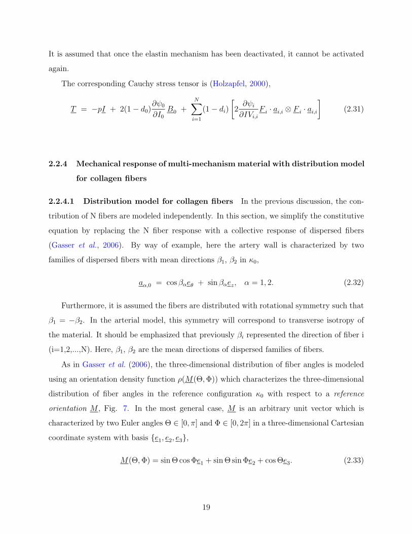
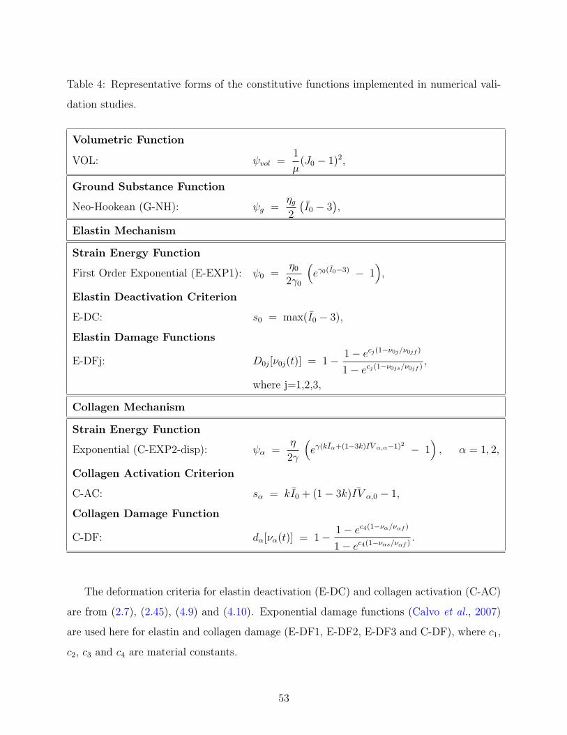
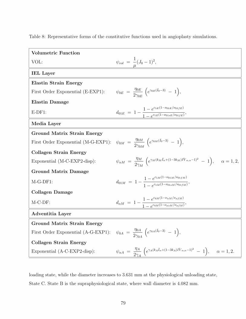
Table 5: Material parameters for an isotropic elastin mechanism (E-EXP1), dispersive anisotropiccollagen mechanism (C-EXP2-disp), volumetric function (VOL) and damage functions (E-DC, E-DF1, E-DF2, E-DF3, C-AC and C-DF), as shown in Table 4.

Material parameters for strain energy functionsµ(Pa−1) η0(KPa) γ0 η(KPa) γ β1 = −β2 k

1e-9 4.55 0.5651 125.0 1.88 56o 0.201

Material parameters for damage functionsc1 c2 c3 c4 ν01s(KPa) ν01f (KPa) ν02s(KPa)

0.25 2.1 10.0 0.002 100.0 250.0 100.0ν02f (KPa) ν03s ν03f ν1s ν1f s1a s0b

2100.0 0.0 1000.0 1.0 2.0 0.5435 3.48

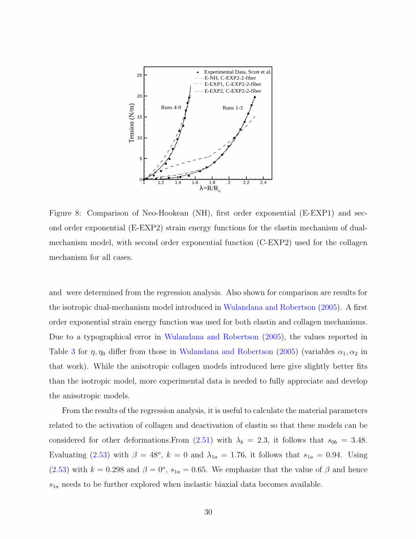
and dα = 0.0) and eventual failure of elastin (point A). In contrast, the cyan curve in

Fig. 11 corresponds to abrupt elastin failure (point B) without progressive damage (e.g. in

Wulandana and Robertson (2005); Li and Robertson (2009)). The blue curve in Fig. 12

corresponds to progressive mechanical damage of elastin based on accumulated equivalent

strain with d0 = d02 (d01 = 0.0, d03 = 0.0 and dα = 0.0) and eventual failure of elastin

(point C). The green curve in Fig. 13 corresponds to the progressive mechanical damage of

elastin and collagen based on maximum equivalent material strain and maximum fiber strain

55

respectively with d0 = d01 and dα = d1 = d2 (d02 = 0.0 and d03 = 0.0). The collagen damage

starts at point D. Only collagen contributes to further loading after the elastin fails at point

E. Eventually, collagen fails at point F. In all cases without collagen damage, after elastin

failure, only collagen contributes to further loading and future loads follow the curve 1. In

all cases, residual stretch is observed upon unloading after elastin failure. The analytical

solutions for these three cases are used to validate the finite element solutions, Figs. 14, 15

and 17.

The finite element solutions for the uniaxial one-step load of the arterial strip with elastin

enzymatic damage arising from hemodynamic loading with d0 = d03 (d01 = 0.0, d02 = 0.0 and

dα = 0.0) are validated with the corresponding analytical solutions, Fig. 16. The solutions

are represented as the axial stress as a function of time. For each curve, the values of WSS

and WSSG are constant and above the threshold value. As expected from the functional

form given in (3.23), the elastin degrades faster for higher levels of WSS and/or WSSG.

As for the case of cyclic damage, Figs. 14, 15 and 17, after elastin failure only collagen

contributes to further loading and future loads follow curve 2. In all cases, the numerical

and analytical solutions match well with a maximum error less than 5%.

4.2.3 Cylindrical inflation and tension of a thick-walled artery

In this section, the analytical solution for the biaxial cylindrical inflation-tension of thick

walled arteries using the structural multi-mechanism model with fiber distribution is for-

mulated. The arterial wall is modeled as a straight wall with constant thickness, composed

of a homogeneous structural multi-mechanism material. The deformation is assumed to be

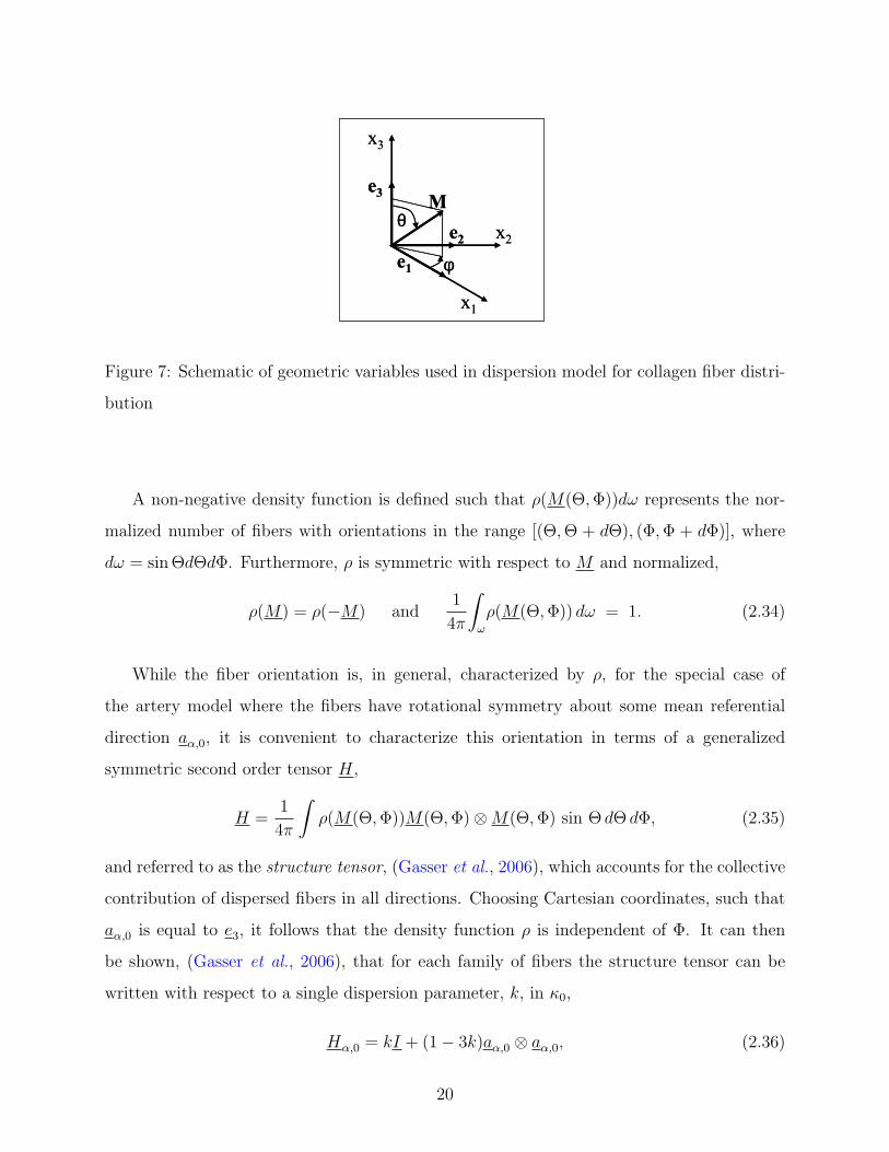
axisymmetric, quasi-static and uniform in the axial direction. To represent the loads on the

arterial wall, pressures pi, po and tension N are applied on the inner surface, outer surface

and axial section of a straight cylinder respectively, Fig. 18. Residual stress is neglected in

this analysis. We first looked for the stress response for a typical material point, and then

the relationship between arterial wall stresses and transmural pressure. In the discussion of

this section, we use the general form of the strain energy functions ψ0(I0) and ψα(Iα, IVα,α).

The specific form of the functions can be found in Section 4.2.1.

56

1 1.5 2 2.50

50000

100000

150000

200000

250000

300000

Elastin cyclic damageand failure

B

A 1

Residual

λ

σ (Pa)Elastin failure withoutcyclic damage

Figure 11: Comparison of two analytical solutions for elastin failure without damage and

elastin cyclic damage d01. Elastin failure at point B and A, respectively, with the remaining

collagen mechanism following load curve 1.

1 1.5 2 2.50

20000

40000

60000

80000

100000

Elastin cyclic damage d02

C

A

1

Residual

λ

σ (Pa) Elastin cyclic damage d01

Figure 12: Comparison of two analytical solutions for elastin cyclic damage d01 and d02.

Elastin failure at point A and C, respectively, with the remaining collagen mechanism fol-

lowing load curve 1.

57

1 1.5 2 2.5 30

20000

40000

60000

80000

100000

Cyclic damage of elastin d01and collagen dα

D

A

1

Residualλ

σ (Pa)

Elastin cyclic damage d01

E

F

Figure 13: Comparison of two analytical solutions for elastin cyclic damage d01 and elastin

cyclic damage d01 with collagen damage dα. For elastin cyclic damage, elastin fails at point

A with the remaining collagen following load curve 1. For elastin and collagen cyclic damage,

elastin fails at point E; collagen starts to experience damage at point D and fails at point F.

1 1.5 2 2.50

20000

40000

60000

80000

100000

Numerical solution

A

1

Residual

λ

σ (Pa) Analytical solution

Figure 14: Comparison of the analytical and numerical solutions for elastin cyclic damage

d01. Elastin failure at point A with the remaining collagen following load curve 1.

58

1 1.5 2 2.50

20000

40000

60000

80000

100000

Numerical solution

CResidual

λ

σ (Pa) Analytical solution

Figure 15: Comparison of the analytical and numerical solutions for elastin cyclic damage

d02. Elastin failure at point C.

2000 4000 6000 80000

100000

200000

300000

400000

Numerical solution

t

σ (Pa) Analytical solution

WSS and/or WSSG 2

Figure 16: Comparison of the analytical and numerical solutions for elastin enzymatic dam-

age d03 for different choices of WSS and/or WSSG. As these quantities are increased, the

elastin degradation occurs more rapidly. The remaining collagen following load curve 2 after

elastin failure.

59

1 1.5 2 2.5 30

20000

40000

60000

80000

100000

Analytical solution

D

Residualλ

σ (Pa)

Numerical solution

E

F

Figure 17: Comparison of the analytical and numerical solutions for elastin cyclic damage

d01 with collagen damage dα. Elastin fails at point E; collagen starts to experience damage

at point D and fails at point F.

N=0.0

pi=0.0

κ0Z

N

κ(t)

N

rori

R

N=0.0

l

pi

Figure 18: Cylinder in unloaded configuration κ0 and loaded configuration κ(t).

60

4.2.3.1 Kinematics and constitutive response During this biaxial deformation as

shown in Fig. 18, the cylindrical arterial wall is inflated and extended. In term of cylindrical

coordinate basis er, eθ, ez, a typical material point at position X0 = R0er + Z0ez in κ0 is

mapped to position x = R(R0, Z)er + Z(Z0)ez in κ(t). The geometry of the cylinder before

and after deformation is defined as,

Ri ≤ R0 ≤ Ro, 0 ≤ Z0 ≤ L, ri ≤ R ≤ ro, 0 ≤ Z ≤ l, (4.36)

in which Ri, Ro, and L denote the undeformed inner radius, outer radius and length respec-

tively, and ri, ro, and l are the corresponding deformed geometrical parameters. It follows

from the incompressibility constraint that,

Z(R2 − r2i ) = Z0(R

20 −R2

i ). (4.37)

The deformation gradient relative to the reference configuration κ0 is,

[F 0] =

1

λΘλZ

0 0

0 λΘ 0

0 0 λZ

=

∂R

∂R0

0 0

0R

R0

0

0 0Z

Z0

, (4.38)

where λΘ = R/R0 is the circumferential stretch, and λZ = Z/Z0 is the axial stretch. Applying

(4.37),

[F 0] =

R0

RλZ

0 0

0R

R0

0

0 0Z

Z0

. (4.39)

The corresponding Cauchy-Green deformation tensors are,

[B0] = [C0] =

1

λ2Θλ2

Z

0 0

0 λ2Θ 0

0 0 λ2Z

, (4.40)

with invariants,

I0 =1

λ2Θλ2

Z

+ λ2Θ + λ2

Z , IV1,0 = IV2,0 = λ2Θ cos2 β + λ2

Z sin2 β. (4.41)

61

Following (2.7) and (2.45), the deformation for elastin deactivation is,

s0 = max(1

λ2Θλ2

Z

+ λ2Θ + λ2

Z − 3), (4.42)

and the measure for collagen activation is,

s1 = s2 = k(1

λ2Θλ2

Z

+1

λ2Θ

+ λ2Z) + (1− 3k)(λ2

Θ cos2 β + λ2Z sin2 β)− 1. (4.43)

We denote λΘa and λZa as the circumferential and axial stretches at which s1 = s2 = sa,

sa = k(1

λ2Θaλ

2Za

+1

λ2Θa

+ λ2Za) + (1− 3k)(λ2

Θa cos2 β + λ2Za sin2 β)− 1, (4.44)

so that from Eq. (4.41),

IV1a,0 = IV2a,0 = λ2Θa cos2 β + λ2

Za sin2 β. (4.45)

Similarly, we denote λΘb and λZb as the circumferential and axial stretches at which s0 = sb,

so that

sb =1

λ2Θbλ

2Zb

+ λ2Θb + λ2

Zb − 3. (4.46)

The kinematic variables relative to reference configuration κα are,

[Fα] =

λΘaλZa

λΘλZ

0 0

0λΘ

λΘa

0

0 0λZ

λZa

, (4.47)

[Bα] = [Cα] =

λ2Θaλ

2Za

λ2Θλ2

Z

0 0

0λ2

Θ

λ2Θa

0

0 0λ2

Z

λ2Za

, (4.48)

with the following invariants,

Iα =λ2

Θaλ2Za

λ2Θλ2

Z

+λ2

Θ

λ2Θa

+λ2

Z

λ2Za

, IVα,α =λ2

Θ cos2 β + λ2Z sin2 β

λ2Θa cos2 β + λ2

Za sin2 β. (4.49)

62

Following (3.26), the measure for collagen damage is,

sα,α = k(λ2

Θaλ2Za

λ2Θλ2

Z

+λ2

Θ

λ2Θa

+λ2

Z

λ2Za

) + (1− 3k)(λ2

Θ cos2 β + λ2Z sin2 β

λ2Θa cos2 β + λ2

Za sin2 β)− 1. (4.50)

The Cauchy stresses can be expressed as in (2.48).

4.2.3.2 Analytical solution for pressure and axial force In the absence of body

forces, the equilibrium equations for the biaxial deformation are,

divt = 0, (4.51)

with boundary conditions,

t = pier at R = ri, t = −poer at R = ro,

t = −Nez at Z = 0, t = Nez at Z = l. (4.52)

Due to the geometrical and constitutive symmetry, the radial componenent of the equilibrium

equations is,∂tRR

∂R+

tRR − tΘΘ

R= 0. (4.53)

By integrating Eq. (4.53) between ri and ro, we can obtain the transmural pressure,

∆p = pi − po =

∫ ro

ri

1

R(tΘΘ − tRR) dR. (4.54)

By definition, the axial force is,

N = πr2i pi + F = 2π

∫ ro

ri

tZZR dR = 2π[

∫ ro

ri

(tZZ − tRR)R dR +

∫ ro

ri

tRRR dR], (4.55)

in which F is the reduced axial force. By integrating by parts the last term of Eq. (4.55)

and applying Eq. (4.53), we have,

∫ ro

ri

tRRR dR =r2i

2pi − r2

o

2po +

∫ ro

ri

(tRR − tΘΘ)R

2dR. (4.56)

63

After substituting Eq. (4.56) into Eq. (4.55), the axial force can be expressed as,

N = πr2i pi + F = πr2

i pi − πr2opo + π

∫ ro

ri

(2tZZ − tRR − tΘΘ)R dR. (4.57)

From Eq. (2.48), the integrands in Eq. (4.54) and (4.57) are,

tΘΘ−tRR = 2(1−d0)∂ψ0

∂I0

(λ2Θ−

1

λ2Θλ2

Z

) +2∑

α=1

(1−dα)

[2∂ψα

∂Iα

(λ2

Θ

λ2Θa

− λ2Θaλ

2Za

λ2Θλ2

Z

) + 2∂ψα

∂IVα,α

λ2Θ cos2 β

IVαa,0

],

(4.58)

2tZZ − tRR − tΘΘ = 2(1− d0)∂ψ0

∂I0

(2λ2Z − λ2

Θ −1

λ2Θλ2

Z

) +2∑

α=1

(1− dα)[2∂ψα

∂Iα

(2λ2

Z

λ2Za

− λ2Θ

λ2Θa

− λ2Θaλ

2Za

λ2Θλ2

Z

)

+ 2∂ψα

∂IVα,α

(λ2Z sin2 β − λ2

Θ cos2 β)

IVαa,0

]. (4.59)

Therefore, N can be evaluated for specific material functions using (4.57) and (4.59). Simi-

larly, ∆p can be determined from (4.54) and (4.58).

4.2.3.3 Comparison of numerical and analytical solutions Using the implemented

structural multi-mechanism model, a three dimensional finite element model was constructed

to obtain the numerical solution for inflation and tension of a cylindrical artery. Due to the

axisymmetric geometry, material and loads, a symmetric cylinder model was used to reduce

the computational cost, Fig. 19. Eight-node solid elements were used for meshing.

Figure 19: Symmetric finite element model for the inflation and tension of cylinder.

64

First, we look at the case in which a monotonic increased biaxial loads are applied.

Constitutive model for elastin failure (E-DC) without cyclic damage is used here. The

geometry and constitutive properties used in these analytical and numerical analyses are

shown in Table 6. Three representative arterial thickness values are considered here in the

range of 100− 200µm, as reported in Scott et al. (1972). The constitutive parameters were

obtained by nonlinear regression analysis of the data of Scott et al. (1972) as in Section 2.3.2.

Table 6: Geometry and material parameters of the validation models, with combinations of firstorder exponential (E-EXP1) strain energy function for the elastin mechanism, second order expo-nential function for the collagen mechanism (C-EXP2-disp), elastin deactivation criterion (E-DC)and collagen activation criterion (C-AC).

Thickness(µm) Ri(mm) Ro(mm) η0(KPa) γ0 η(KPa) γ k β1 = −β2 s1a s0b

100 0.28 0.38 9.09 0.5652 252.0 1.91 0.199 56.7 0.5377 3.48150 0.28 0.43 6.06 0.5651 167.9 1.90 0.200 56.5 0.5401 3.48200 0.28 0.48 4.55 0.5651 125.0 1.88 0.201 56.2 0.5435 3.48

Fig. 20 shows the analytical solution (4.54) for transmural pressure (∆p) as a function of

inner circumferential stretch λΘi during the biaxial inflation and tension of a 200 µm thick

cylinder. Two solutions with different inner radial stretch were presented. The axial stretch

is the same for both cases: λZ = 1.2. The start point for elastin degradation can be observed

from the load curves, at which λΘi = λΘb, λZi = λZb. Numerical oscillation can be observed

on the load curves after the material starts a continuous degradation of the elastin.

The comparison of analytical solution and finite element solution for this biaxial inflation-

tension analysis is shown in Figs. 21 and 22. Fig. 21 shows the result of a mesh density

study in the cylinder thickness direction. Three simulation cases are compared with the

analytical solutions using different mesh size. It is found that 100 elements are needed to

obtain an accurate solution compared with the analytical one for the error to be less than 5%

in this case. Fig. 22 shows the impact of the material compressibility parameter on the finite

element solution. Three compressibility parameters are used for different cases, in which the

case using µ = 10−9Pa−1 is shown to match the analytical solution well with the error less

than 5%. It is shown that the compressibility parameter is critical for obtaining satisfactory

numerical solution compared with analytical solution for the modeling of incompressible

material.

65

1 1.5 2 2.5 3 3.50

10000

20000

30000

40000

λθi=λθb

∆p (Pa)

λθi=ri / Ri

(a)

1 1.5 2 2.5 3 3.5 40

50000

100000

150000

200000

250000

300000

λθi=ri / Ri

λθi=λθb

∆p (Pa)

(b)

Figure 20: Analytical solution for biaxial inflation-tension of 200 µm thick cylinder for two

values of circumferential stretch: (a) λΘi = 3.0 and (b) λΘi = 3.6.

1 1.5 2 2.5 3 3.50

10000

20000

30000

40000

analytical solution

20 elements10 elements

100 elements

∆p (Pa)

λθi=ri / Ri

Figure 21: Comparison of analytical solution and numerical solution for biaxial inflation-

tension of 200 µm thick cylinder with λΘi = 3.0 and λZ = 1.2. Study of mesh density.

66

1 1.5 2 2.5 3 3.50

10000

20000

30000

40000

Analytical solution

∆p (Pa)

λθi=ri / R i

µ=10-9 Pa-1

µ=10-7 Pa-1

µ=10-6 Pa-1

Figure 22: Comparison of analytical solution and numerical solution for biaxial inflation-

tension of 200 µm thick cylinder with λΘi = 3.0 and λZ = 1.2. Study of incompressiblity.

Fig. 23 shows the comparison of finite element solution and analytical solution for the

biaxial inflation-tension analysis with circumferential stretch λΘi = 3.6 and axial stretch

λZ = 1.2. 100 elements are used through the cylinder thickness and a compressibility

parameter µ = 10−12Pa−1 is used in the analysis. The numerical solution converges to the

analytical solution well.

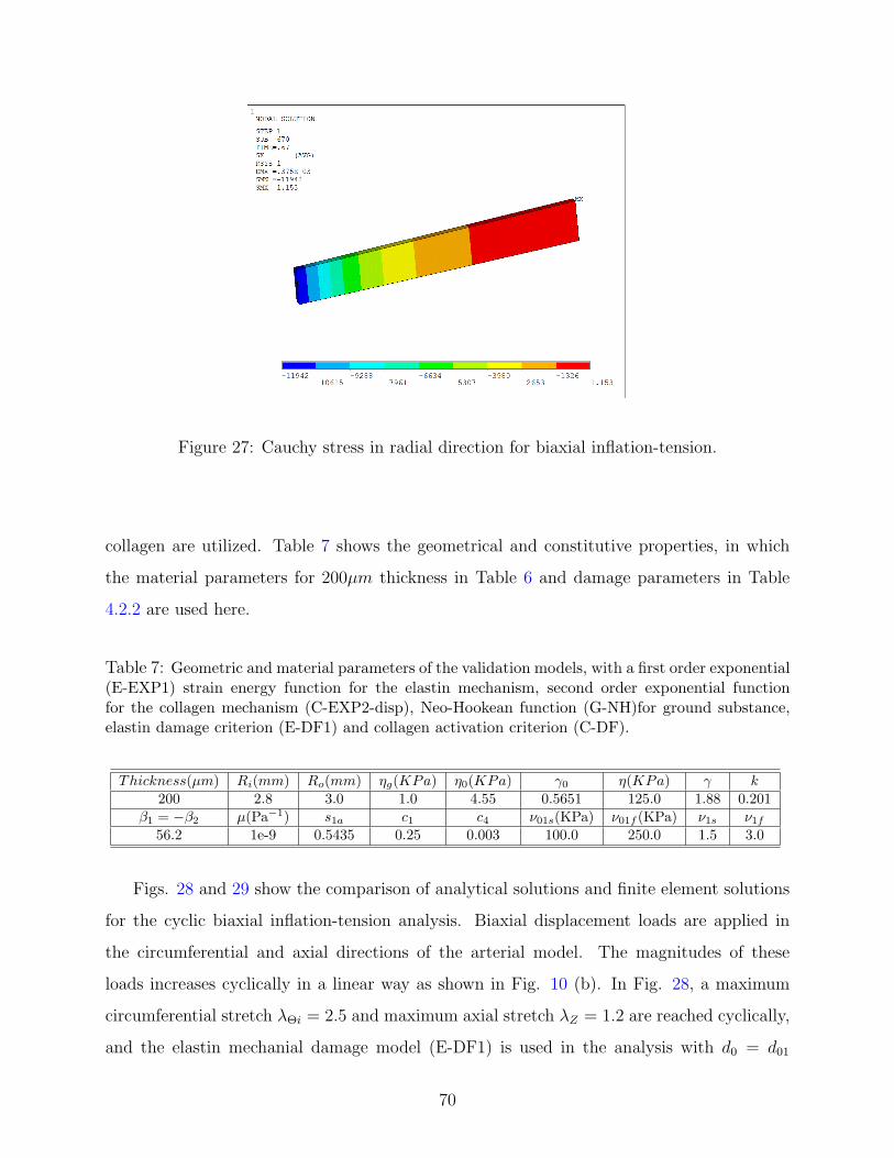
Figs. 24-27 show some simulation results at one loading stage of the biaxial inflation-

tension analysis. Fig. 24 shows the current collagen recruitment status through the cylinder

thickness, in which a value of one corresponds to no collagen fiber recruitment and a value

of zero represents recruited collagen fibers. Fig. 25 shows the current elastin degradation

status through the cylinder thickness. Here, a value of one represents complete degradation

or failure of elastin and a value of zero represents complete undegradated elastin. Fig. 26

visualizes the mean orientation distribution of the fiber families. The Cauchy stress in the

radial direction is shown in Fig. 27.

Secondly, we investigate the case in which cyclically increasing biaxial loads are applied

to the cylindrical model. Constitutive models for cyclic damage behavior of both elastin and

67

1 1.5 2 2.5 3 3.5 40

50000

100000

150000

200000

250000

300000

Numerical solution

Analytical solution∆p (Pa)

λθi=ri / Ri

Figure 23: Comparison of analytical solution and numerical solution for biaxial inflation-

tension of 200 µm thick cylinder with λΘi = 3.6 and λZ = 1.2.

0 = recruitment1 = no recruitment

Figure 24: Collagen fiber recruitment status for biaxial inflation-tension of 200 µm thick

cylinder with circumferential stretch λΘi = 3.0 and axial stretch λZ = 1.2.

68

0 = no degradation1 = complete degradation

Figure 25: Elastin degradation status for biaxial inflation-tension.

Figure 26: Mean orientation of collagen fiber family for biaxial inflation-tension.

69

Figure 27: Cauchy stress in radial direction for biaxial inflation-tension.

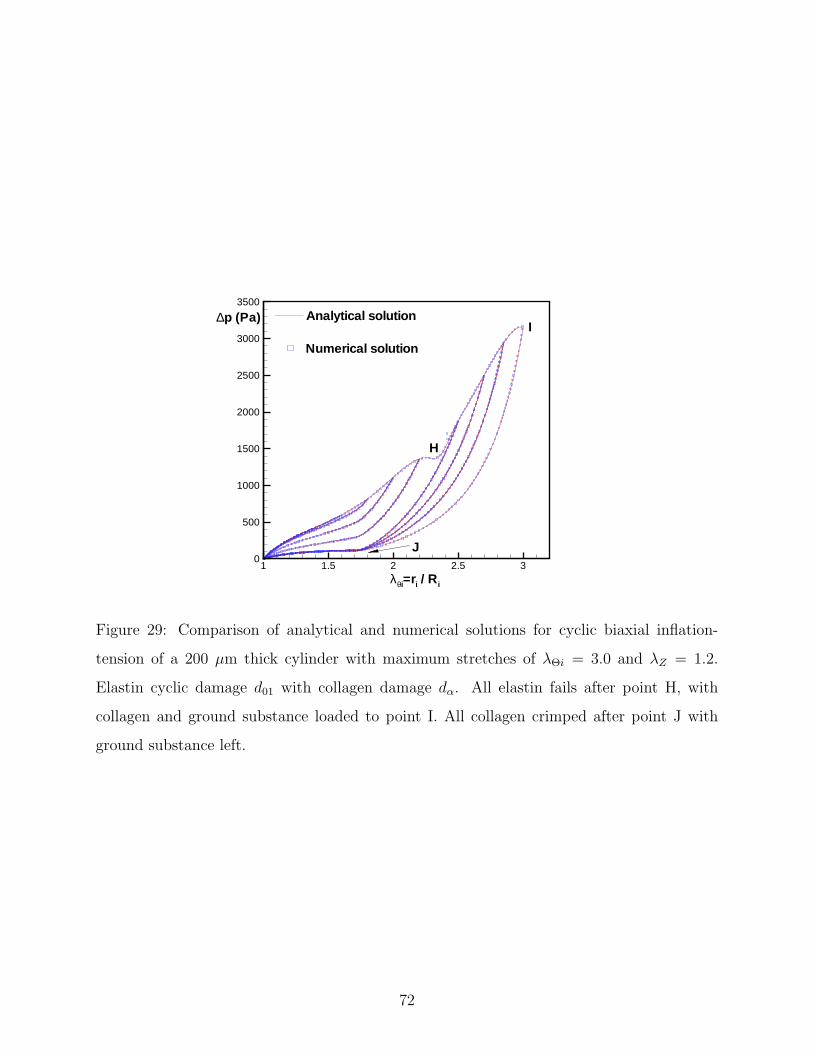
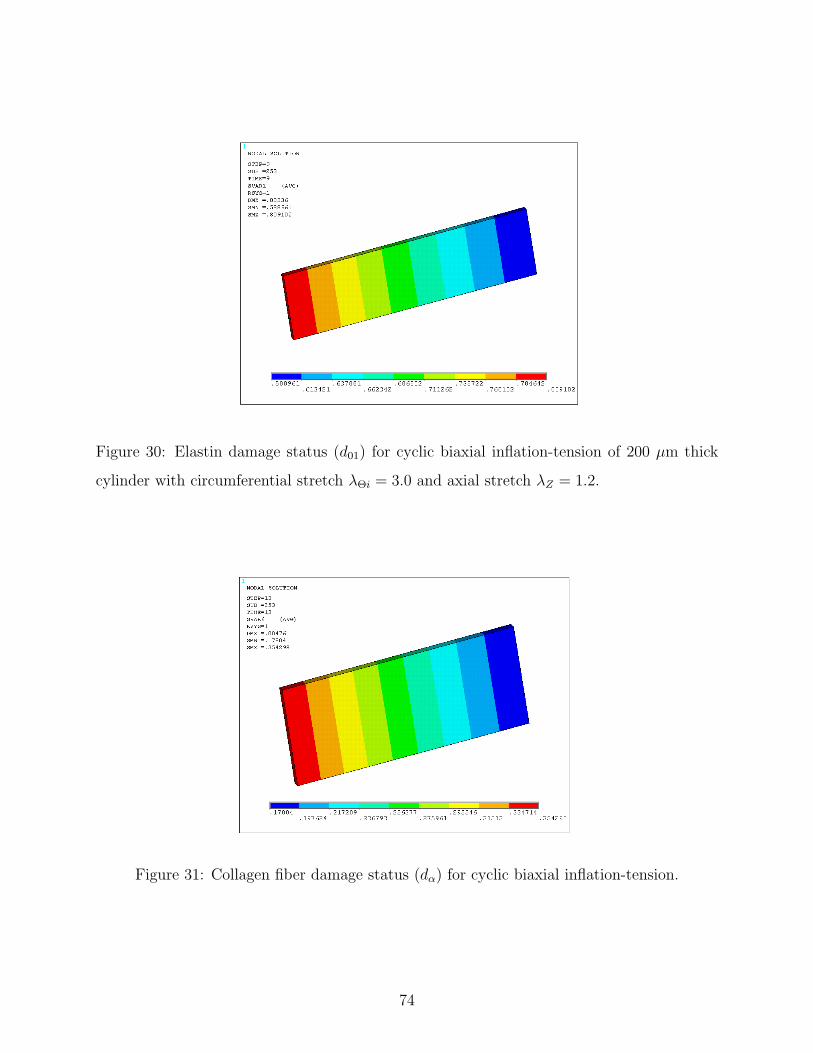
collagen are utilized. Table 7 shows the geometrical and constitutive properties, in which

the material parameters for 200µm thickness in Table 6 and damage parameters in Table

4.2.2 are used here.

Table 7: Geometric and material parameters of the validation models, with a first order exponential(E-EXP1) strain energy function for the elastin mechanism, second order exponential functionfor the collagen mechanism (C-EXP2-disp), Neo-Hookean function (G-NH)for ground substance,elastin damage criterion (E-DF1) and collagen activation criterion (C-DF).

Thickness(µm) Ri(mm) Ro(mm) ηg(KPa) η0(KPa) γ0 η(KPa) γ k200 2.8 3.0 1.0 4.55 0.5651 125.0 1.88 0.201

β1 = −β2 µ(Pa−1) s1a c1 c4 ν01s(KPa) ν01f (KPa) ν1s ν1f

56.2 1e-9 0.5435 0.25 0.003 100.0 250.0 1.5 3.0

Figs. 28 and 29 show the comparison of analytical solutions and finite element solutions

for the cyclic biaxial inflation-tension analysis. Biaxial displacement loads are applied in

the circumferential and axial directions of the arterial model. The magnitudes of these

loads increases cyclically in a linear way as shown in Fig. 10 (b). In Fig. 28, a maximum

circumferential stretch λΘi = 2.5 and maximum axial stretch λZ = 1.2 are reached cyclically,

and the elastin mechanial damage model (E-DF1) is used in the analysis with d0 = d01

70

1 1.5 2 2.50

500

1000

1500

2000

Analytical solution

Residual

λθi=ri / Ri

∆p (Pa)

Numerical solution

G

3

Figure 28: Comparison of analytical and numerical solutions for cyclic biaxial inflation-

tension of a 200 µm thick cylinder with maximum stretches of λΘi = 2.5 and λZ = 1.2 for

elastin cyclic damage d01. All elastin fails after point G with collagen left following load

curve 3.

71

1 1.5 2 2.5 30

500

1000

1500

2000

2500

3000

3500

Analytical solution

λθi=ri / Ri

∆p (Pa)

Numerical solution

H

J

I

Figure 29: Comparison of analytical and numerical solutions for cyclic biaxial inflation-

tension of a 200 µm thick cylinder with maximum stretches of λΘi = 3.0 and λZ = 1.2.

Elastin cyclic damage d01 with collagen damage dα. All elastin fails after point H, with

collagen and ground substance loaded to point I. All collagen crimped after point J with

ground substance left.

72

(d02 = 0.0, d03 = 0.0 and dα = 0.0). Elastin is damaged progressively through the cylinder

thickness. All elastin fails after point G and only collgen is left following load curve 3.

Residual stretch is observed upon unloading.

In Fig. 29, maximum circumferential stretch is λΘi = 3.0, maximum axial stretch is

λZ = 1.2, and the elastin mechanical damage model (E-DF1) is used together with the

collagen damage model (C-DF), so d0 = d01 and dα = d1 = d2 (d02 = 0.0 and d03 = 0.0)

here. For the purpose of numerical test, an undamaged ground substance is also utilized here

as one material component to hold the cyclic loads especially when large damage of elastin

and collagen happens. Both elastin and collagen are damaged progressively with complete

elastin failure at point H. Collagen and ground substance are cyclically loaded until point I

after elastin failure. During the unloading, all collagen is unrecruited after point J with only

ground substance left. 100 solid elements are used through the cylinder thickness in both

analyses. The numerical and analytical solutions match well with maximum errors less than

5%.

Figs. 30 and 31 show the current elastin (d01) and collagen fiber (dα) damage status

respectively through the cylinder thickness at one loading stage of the cyclic biaxial inflation-

tension analysis. Here, a value of one represents complete degradation or failure, a value

of zero represents undamaged status, and a value between zero and one corresponds to the

varying degrees of damage of elastin or collagen fibers.

73

Figure 30: Elastin damage status (d01) for cyclic biaxial inflation-tension of 200 µm thick

cylinder with circumferential stretch λΘi = 3.0 and axial stretch λZ = 1.2.

Figure 31: Collagen fiber damage status (dα) for cyclic biaxial inflation-tension.

74

5.0 MODELING OF CEREBRAL ANGIOPLASTY

5.1 INTRODUCTION

Percutaneous transluminal angioplasty (PTA) is performed to treat atherosclerotic obstruc-

tion and vasospasm in cerebral vessels (Wojak et al., 2006; Higashida et al., 1992; Honma

et al., 1995), with the primary mechanical mechanism explained as the overstretching and

widening of arterial wall layers: intima, media and adventitia (Castaneda-Zuniga et al.,

1980). PTA can introduce direct vascular damage by the deployment of balloon, stent and

cerebral protection devices (Muller-Hulsbeck et al., 2005). Transluminal dilatation of small

and fragile intracranial arteries is more dangerous than that of extracranial arteries when

overstretched. Visible vessel wall damage is observed at the site of PTA, characterized by

intimal damage (endothelial damage, subendothelial destruction, fractured IEL) and medial

changes (damaged myocytes, loss of dense bodies, gaps in the extracellular matrix, disorga-

nized collagen fibers) (Castaneda-Zuniga et al., 1981; Zollikofer et al., 1984; Chavez et al.,

1990; Honma et al., 1995; Connors and Wojak, 1999). These unusual morphological changes

are usually absent in the distal arterial segments on which PTA has not been carried out.

Despite reparative processes including endothelial regeneration, damage of the internal

elastic lamina (IEL) and media are grossly irreversible in the damaged region (Zollikofer

et al., 1984; Chavez et al., 1990; Castaneda-Zuniga et al., 1980). Intimal damage can lead

to malignant thrombus/platelet aggregation progressing to total occlusion since intracranial

vessels are relatively small and can be extremely thrombogenic (Connors and Wojak, 1999).

In addition to such minor structural damages as areas of disruption and dissection throughout

the vessel layers, major structural damage including partial tears of intima or media, splitting

of atheromatous plaques and hemorrhages may result in stroke, and even a tear or rupture

75

of the vessel wall (Honma et al., 1995; Connors and Wojak, 1999). However, the damage to

the vessel wall following PTA has not been rigorously investigated.

In a controlled study of angioplasty in common carotid, iliac, and femoral arteries of

mongrel dogs, changes to the arterial wall due to over inflation were studied at two dilation

levels (25%, 50%) (Zollikofer et al., 1984). Damage to the wall was progressive increasing

with inflation level. At 25% inflation, localized fractures and stretching of the IEL were

observed. Damage to the media was limited to the inner one-third of the wall. At 50%

inflation, further radial damage was seen including extensive damage to the IEL, dissection of

the media, distorted SMC and disorganized collagen fibers through more than half the media.

The changes were most pronounced in the inner layers and decreased towards the outer layers

of the wall. At six months, the media exhibited signs of repair such as regeneration of smooth

muscle cells and increased collagen contents in formerly dilated areas while the IEL showed

no recovery, not even in places where it had been destroyed. For the long-lasting effects of

PTA, the effects of growth and remodeling will be important such as intimal hyperplasia

and fibrotic changes of the media in the dilated arterial wall (Zollikofer et al., 1984; Honma

et al., 1995).

Arterial inelastic deformations including elastoplastic and damage mechanisms are im-

portant phenomena during supraphysiological loading such as mechanical treatments like

PTA (Holzapfel et al., 2000). From mechanical test of arteries (Holzapfel et al., 2000; Ok-

tay et al., 1991), it was shown that mechanical damage results in significant changes in the

mechanical behavior such as tissue softening (weakening) and non-recoverable deformation.

The residual stretches are responsible for the luminal increase during PTA and are described

as “controlled vessel injury” (Castaneda-Zuniga et al., 1985).

Here, we simulate cerebral arterial angioplasty surgery using the structural damage model

and use this simulation tool to analyze arterial tissue injury. A three-dimensional computa-

tional model of artery and balloon is built to simulate the artery-balloon interaction during

an angioplasty procedure. A multi-step simulation scheme is utilized including the inflation-

tension of artery, inflation of balloon and the contact between artery and balloon. Due to

the extensive computational requirements for contact analysis with nonlinear materials, we

use an axisymmetric model for the simulation. To characterize cerebral arteries, we build

76

a multi-layer artery model composed of the IEL, media and adventitia layers. Heteroge-

neous multi-mechanism materials including elastin, ground matrix and collagen are utilized

for the arterial layers. A more rigid material model is used for balloon model. Related

computational work can be found in Sidorov (2006); Gasser and Holzapfel (2007), in which

Sidorov (2006) simulated angioplasty using a one-layer arterial model with isotropic multi-

mechanism material (Wulandana and Robertson, 2005), and Gasser and Holzapfel (2007)

analyzed angioplasty using an elastoplastic material formulation for arteries.

5.2 FINITE ELEMENT MODEL OF CEREBRAL ANGIOPLASTY

For the modeling of cerebral PTA, first we analyze the high pressure response of a multi-

layer cerebral artery model. Then we use this artery model to simulate the artery-balloon

interaction and tissue injury during cerebral PTA. The PTA pressure is estimated to be

about 1.0 to 1.5 atm (Honma et al., 1995). The balloon is usually undersized by 0.2 to

0.7 mm compared with the diameter of the vessel. Most lesions undergoing dilation are

less than 10 mm long (usually 2 to 4 mm), and thus very short balloons are necessary. A

typical intracerebral single-lumen angioplasty catheter is mostly 2 mm (diameter) by 10 mm

(length) in size (Connors and Wojak, 1999).

5.2.1 High pressure response of a multi-layer arterial model

To represent the heterogeneous histological structure of cerebral arteries (Finlay et al., 1995),

we build a cylindrical arterial model with three layers: the IEL, media and adventitia, Fig.

32. The unloaded internal diameter is 2.3 mm with a total wall thickness of 125 µm. The

IEL, media and adventitia occupy 1/10, 6/10 and 3/10 of the wall thickness respectively. For

constitutive models, we use isotropic elastin material with damage for the IEL, and use the

structural multi-mechanism model for ground matrix and collagen fibers in the media and

adventitia. The fiber orientation for collagen families in the media is 7◦ here, representing

nearly circumferential fiber families, while the mean fiber orientation for collagen families in

77

the adventitia is 56◦ to represent more dispersed fibers (Finlay et al., 1995). Vessel injury

is characterized by damage of elastin, ground matrix and collagen fibers in the IEL and

media, representing intima and media damage. The adventitial collagen and ground matrix

are assumed to be purely elastic since few acute vessel injury is observed in the adventitia

(Zollikofer et al., 1984; Honma et al., 1995). The representative constitutive equations used

in the following simulations are shown in Table 8, in which the mechanical strain-based

damage mechanism is utilized for elasin/ground matrix and collagen damage.

Figure 32: Cylindrical multi-layer artery model for biaxial inflation-tension.

We first simulate the high pressure response of the multi-later arterial wall. Material

parameters used in this simulation are shown in Table 9. Since there is no experimental data

available for individual layers of cerebral arteries, we choose the elastic parameters based on

values from previous studies in Section 2.3.2 and Li and Robertson (2009); Li and Robertson

(2009b). The damage parameters are chosen to ensure that large damage response happens

in arterial layers during the typical PTA pressures and physically meaningful results are

obtained. With a fixed axial stretch of 1.1, increased internal pressure is applied on the

artery wall from zero to one bar, then unloaded to zero. Fig. 33 shows the loading and

unloading curves for transmural pressure with change of arterial internal diameter. Vessel

wall damage and weakening is clearly shown from the dissipation of loading-unloading curves,

and also the wall diameter changes which is responsible for luminal increase after PTA. As

shown in Fig. 33, the artery has a diameter of 3.480 mm at State A which is the physiological

78

Table 8: Representative forms of the constitutive functions used in angioplasty simulations.

Volumetric Function

VOL: ψvol =1

µ(J0 − 1)2,

IEL Layer

Elastin Strain Energy

First Order Exponential (E-EXP1): ψ0E =η0E

2γ0E

(eγ0E(I0−3) − 1

),

Elastin Damage

E-DF1: d01E = 1− 1− ec1E(1−ν01E/ν01fE)

1− ec1E(1−ν01sE/ν01fE),

Media Layer

Ground Matrix Strain Energy

First Order Exponential (M-G-EXP1): ψ0M =η0M

2γ0M

(eγ0M (I0−3) − 1

),

Collagen Strain Energy

Exponential (M-C-EXP2-disp): ψαM =ηM

2γM

(eγM (kM Iα+(1−3kM ) ¯IV α,α−1)2 − 1

), α = 1, 2,

Ground Matrix Damage

M-G-DF1: d01M = 1− 1− ec1M (1−ν01M/ν01fM )

1− ec1M (1−ν01sM/ν01fM ),

Collagen Damage

M-C-DF: dαM = 1− 1− ec4M (1−ναM/ναfM )

1− ec4M (1−ναsM/ναfM ),

Adventitia Layer

Ground Matrix Strain Energy

First Order Exponential (A-G-EXP1): ψ0A =η0A

2γ0A

(eγ0A(I0−3) − 1

),

Collagen Strain Energy

Exponential (A-C-EXP2-disp): ψαA =ηA

2γA

(eγA(kAIα+(1−3kA) ¯IV α,α−1)2 − 1

), α = 1, 2.

loading state, while the diameter increases to 3.631 mm at the physiological unloading state,

State C. State B is the supraphysiological state, where wall diameter is 4.082 mm.

79

The distribution of circumferential Cauchy stress across the deformed wall thickness is

shown in Figs. 34, 35 and 36 for States A, B and C respectively. It is shown that the IEL,

media and adventitia layers have discontinuous stress distributions and stress gradients. The

IEL stress level is the lowest for all three states. At State A, the highest wall stress is found

in the media layer. This high stress shifts to the adventitia layer at States B and C, which

is due to the inelastic damage in the media and stiffening of the adventitia from collagen

recruitment during high pressure loading. The stress gradient in the media changes greatly

from State A to States B and C, which is due to the nonhomogenerous damage accumulating

across the media layer.

Table 9: Material parameters for three arterial layers in high-pressure response.

µ(Pa−1) η0E(KPa) γ0E c1E ν01sE(KPa) ν01fE(KPa) η0M (KPa) γ0M c1M

1e-8 4.55 0.565 0.12 75.0 120.0 4.55 0.565 0.12ν01sM (KPa) ν01fM (KPa) ηM (KPa) γM βM kM c4M ναsM ναfM

75.0 120.0 125.0 1.88 7◦ 0.0 0.0025 1.3 2.5sαaM η0A(KPa) γ0A ηA(KPa) γA βA kA sαaA

0.5435 0.51 5.086 125.0 1.88 56◦ 0.201 0.51

5.2.2 Simulation of balloon-artery interaction during cerebral angioplasty

In this section, we simulate cerebral angioplasty using the multi-layer artery model and a

balloon model, Fig. 37. We use a axisymmetric model with fore-aft symmetry so only part

of the arterial segment and balloon are included in the computational model. The artery

has an unloaded internal diameter of 2.5 mm (3.816 mm at the physiological loading state),

a thickness of 125 µm and a length of 10 mm. The balloon has a external diameter of 1.8

mm and a length of 5 mm. The interaction between artery and balloon is simulated using

a surface contact strategy. The model has 17000 3D solid elements, 2600 contact elements

and four solid materials: balloon, IEL, media and adventitia. Material parameters used for

arterial layers are shown in Table 10. Compared to the material parameters in Table 9, the

elastic properties of the adventitia are modified to make the adventitia much stiffer than

the media at high pressures, while keep the media stiffer at low pressures (Yu et al., 1993;

Holzapfel et al., 2005). The damage properties of the IEL and media are also adjusted to

80

2 2.5 3 3.5 4 4.50

20

40

60

80

100

Inner diameter di (mm)

Tra

nsm

ural

pres

sure

∆p(K

Pa)

Physiological loading domain

A C

B

3.48

03.

631

4.08

2

Figure 33: High pressure response of the multi-layer artery model for biaxial inflation-tension

with axial stretch λZ = 1.1 and internal pressure increased from 0 to 1 bar (State B), then

unloaded to 0.

0 20 40 600

100

200

300

400

500

r-r i (µm)

Cau

chy

stre

ssσ θθ

(KP

a)

IEL Media Adventitia

Figure 34: Circumferential Cauchy stress distribution across the deformed wall thickness at

State A.

81

0 10 20 30 40 50 60

0

2000

4000

6000

8000

10000

r-r i (µm)

Cau

chy

stre

ssσ θθ

(KP

a)

IEL Media Adventitia

Figure 35: Circumferential Cauchy stress distribution across the deformed wall thickness at

State B.

0 10 20 30 40 50 60 70

0

100

200

300

400

500

600

r-r i (µm)

Cau

chy

stre

ssσ θθ

(KP

a)

IEL Media Adventitia

Figure 36: Circumferential Cauchy stress distribution across the deformed wall thickness at

State C.

82

ensure a wider range of inelastic response during the more stringent angioplasty loads. A

more rigid Neo-Hookean material is used for the balloon.

Adventitia

Media

IEL

Balloon

Endothelium

Figure 37: Balloon and artery model for cerebral angioplasty simulation.

Table 10: Material parameters for three arterial layers in balloon-artery interaction.

µ(Pa−1) η0E(KPa) γ0E c1E ν01sE(KPa) ν01fE(KPa) η0M (KPa) γ0M c1M

1e-8 4.55 0.565 2.1 80.0 2100.0 4.55 0.565 1.8ν01sM (KPa) ν01fM (KPa) ηM (KPa) γM βM kM c4M ναsM ναfM

100.0 1800.0 125.0 1.88 7◦ 0.0 0.006 1.5 6.0sαaM η0A(KPa) γ0A ηA(KPa) γA βA kA sαaA

0.5435 2.27 1.13 500.0 7.53 56◦ 0.201 0.51

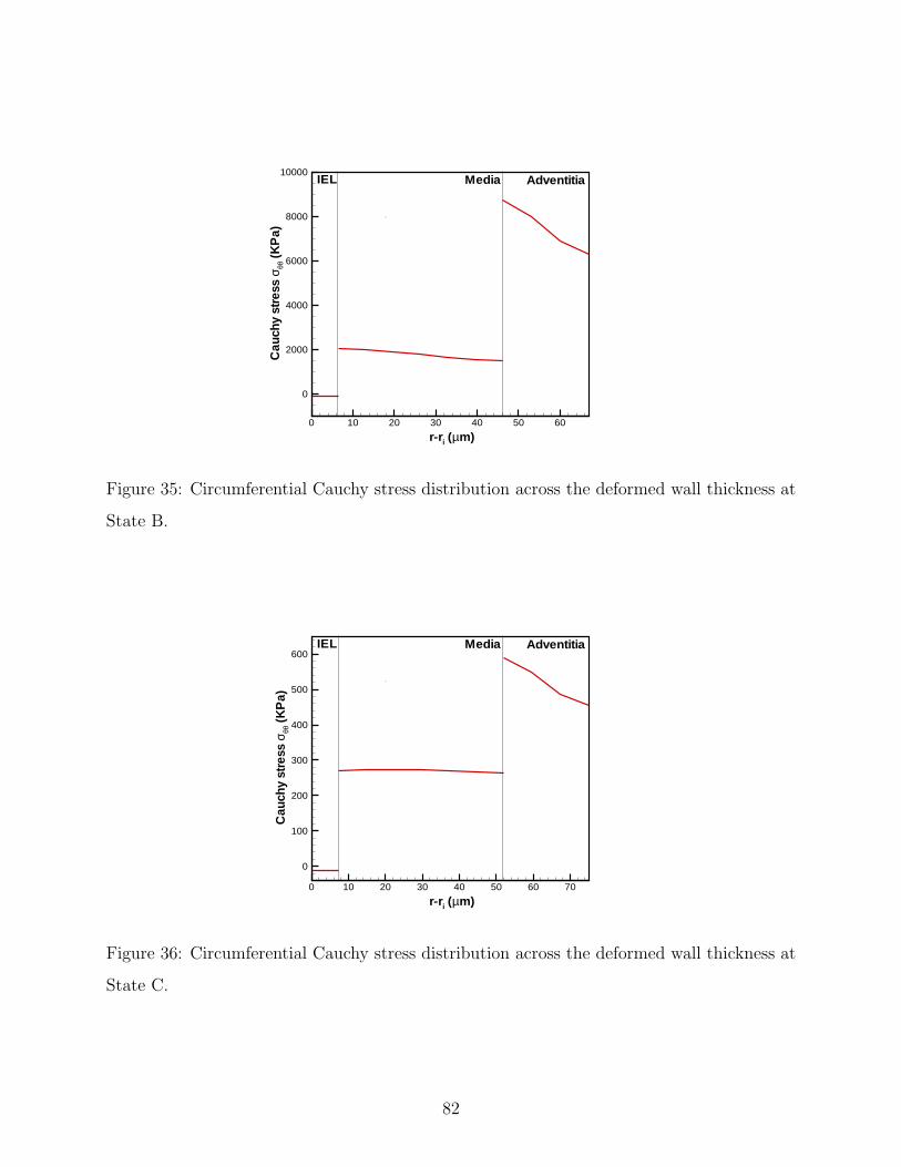
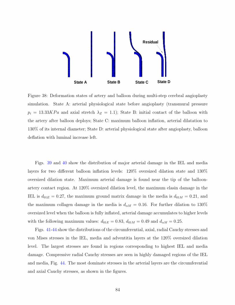
We use a multi-step loading procedure for the angioplasty simulation, with the four

deformation states shown in Fig. 38. First, the artery is inflated to a transmural pressure

∆p = 13.33KPa with an axial stretch λZ = 1.1. This generates the arterial physiological

deformation state before PTA (State A), which is associated with purely elastic response

of arteries. Then, the balloon is deployed to contact and dilate the artery to 130% of

its internal diameter by applying radial displacement loads on the balloon (States B-C).

The inelastic damage and injury of arteries happen during this oversized dilatation process.

Finally, the ballon is unloaded to bring the artery back to its physiological state after PTA

(State D). At this final state, remaining deformation of the artery is found characterized by

nonhomogenerous luminal increase, which is due to the nonrecoverable inelastic damage of

the IEL and media induced by the supraphysiological loading.

83

State A State B State DState C

Residual

Figure 38: Deformation states of artery and balloon during multi-step cerebral angioplasty

simulation. State A: arterial physiological state before angioplasty (transmural pressure

pi = 13.33KPa and axial stretch λZ = 1.1); State B: initial contact of the balloon with

the artery after balloon deploys; State C: maximum balloon inflation, arterial dilatation to

130% of its internal diameter; State D: arterial physiological state after angioplasty, balloon

deflation with luminal increase left.

Figs. 39 and 40 show the distribution of major arterial damage in the IEL and media

layers for two different balloon inflation levels: 120% oversized dilation state and 130%

oversized dilation state. Maximum arterial damage is found near the tip of the balloon-

artery contact region. At 120% oversized dilation level, the maximum elasin damage in the

IEL is d01E = 0.27, the maximum ground matrix damage in the media is d01M = 0.21, and

the maximum collagen damage in the media is dαM = 0.16. For further dilation to 130%

oversized level when the balloon is fully inflated, arterial damage accumulates to higher levels

with the following maximum values: d01E = 0.83, d01M = 0.49 and dαM = 0.25.

Figs. 41-44 show the distributions of the circumferential, axial, radial Cauchy stresses and

von Mises stresses in the IEL, media and adventitia layers at the 120% oversized dilation

level. The largest stresses are found in regions corresponding to highest IEL and media

damage. Compressive radial Cauchy stresses are seen in highly damaged regions of the IEL

and media, Fig. 44. The most dominate stresses in the arterial layers are the circumferential

and axial Cauchy stresses, as shown in the figures.

84

(a) IEL and media (b) media (c) media

max

dαMd01E d01M

maxmax

Figure 39: Damage distribution in the arterial layers at 120% oversized dilation state. The

arrows indicate the locations of the maximum damage: (a) maximum elastin damage in

the IEL d01E = 0.27; (b) maximum ground matrix damage in the media d01M = 0.21; (c)

maximum collagen damage in the media dαM = 0.16.

(a) IEL and media (b) media (c) media

max

dαMd01E d01M

max max

Figure 40: Damage distribution in the arterial layers at 130% oversized dilation state. The

arrows indicate the locations of the maximum damage: (a) maximum elastin damage in

the IEL d01E = 0.83; (b) maximum ground matrix damage in the media d01M = 0.49; (c)

maximum collagen damage in the media dαM = 0.25.

85

(a) IEL (b) media (c) adventitia

maxmaxmax

σθθ(Pa)σθθ(Pa) σθθ(Pa)

Figure 41: Distribution of the circumferential Cauchy stresses in the IEL, media and ad-

ventitia layers at 120% oversized dilation state. The arrows indicate the locations of the

maximum values.

(a) IEL (b) media (c) adventitia

maxmaxmax

σeqv(Pa)σeqv(Pa) σeqv(Pa)

Figure 42: Distribution of the von Mises stresses in the IEL, media and adventitia layers at

120% oversized dilation state. The arrows indicate the locations of the maximum values.

86

(a) IEL (b) media (c) adventitia

maxmax

max

σzz(Pa)σzz(Pa) σzz(Pa)

Figure 43: Distribution of the axial Cauchy stresses in the IEL, media and adventitia layers

at 120% oversized dilation state. The arrows indicate the locations of the maximum values.

(a) IEL (b) media (c) adventitia

neg.maxneg.

σrr(Pa)σrr(Pa) σrr(Pa) maxmax

Figure 44: Distribution of the radial Cauchy stresses in the IEL, media and adventitia layers

at 120% oversized dilation state. The arrows indicate the locations of the maximum values

or negative stresses.

87

6.0 CONCLUSIONS AND DISCUSSIONS

A structural multi-mechanism damage model for cerebral arterial tissue (Li and Robertson,

2009b) has been developed that builds on a previous isotropic multi-mechanism model (Wu-

landana and Robertson, 2005) and a recent generalized anisotropic model (Li and Robertson,

2008, 2009). To characterize elastin failure and collagen in aneurysm formation, the cerebral

arterial tissue is modeled as nonlinear, inelastic and incompressible with separate mecha-

nisms for elastin and collagen in these models. Motivated by structural data on collagen

fiber orientation in cerebral arteries (Finlay et al., 1995), an anisotropic mechanism is rep-

resented by helical networks of crimped collagen fibers in the unloaded arterial wall. The

collective response of fibers is modeled using a distribution function for fiber orientation

(Spencer , 1984; Gasser et al., 2006). The collagen fibers require a finite deformation to be-

gin load bearing. The fiber activation criterion is a function of the local stretch of material

elements tangent to the crimped fiber direction in the unloaded configuration.

As for most other mechanical models of the arterial wall, we take a continuum approach.

It is assumed that the fibers can be approximated as continuously distributed throughout

the material (or arterial layer) so that the fiber orientation vector and other quantities have

meaning at each point in the material and are continuous functions of position. We do not

account for microscopic effects in the composite such as interactions between the fibers and

the matrix or coupling between the collagen fibers, or between the fiber families.

In the analysis here, all fiber families at each material point are assumed to have ap-

proximately the same level of waviness (sa is a constant for all fibers at a point). In some

soft tissue, the degree of fiber undulation can vary considerably with position (Sacks, 2003).

If warranted by experimental data, it is straightforward to generalize the current model to

account for this type of material inhomogeneity. This can be achieved by making sa a func-

88

tion of position. Furthermore, it is assumed that collagen fibers are completely uncrimped

at a discrete loading level s = sa. This can be generalized by introducing an integral model

for fiber recruitment.

It is assumed that all isotropic contributions of the wall are dependent on strain measured

relative to κ0. It is expected that this contribution will primarily come from elastin. The

degradation of this mechanism, which we refer to as the elastin mechanism, is considered

as arising from two possible modes of damage. In the first type, elastin degradation is

dependent on two local measures of strain: a maximum equivalent strain as well as an

accumulated equivalent strain. In the second mode of damage, elastin degradation arises

indirectly from hemodynamic loading. We expect that pathological levels of the wall shear

stress vector initiate a cascade of biochemical activities that lead to degradation of the wall,

rather than directly damaging the elastin. For example, some aspects of the wall shear

stress vector may lead to an imbalance in the production of MMPs and tissue inhibitor of

metalloproteinases (TIMPs) which break down the elastin in the IEL. While at this point,

the specific hemodynamic factors remain to be determined, preliminary studies suggest that

elevated WSS and elevated (positive) WSSG can lead to IEL degradation in native and non-

native bifurcations (Morimoto et al., 2002; Meng et al., 2006). We have given a representative

functional form for the dependence of this second mode of damage on hemodynamic variables

here.

In the proposed model, the two damage mechanisms are coupled in a multiplicative

manner. An elastin layer previously weakened by biochemical factors will undergo larger

deformations for the same physiological load. This can in turn lead to increased mechanical

damage. Since cerebral aneurysms can form in the absence of hypertension, we anticipate

the role of elevated hemodynamic pressures in aneurysm formation is to hasten mechanical

damage of an IEL previously weakened by biochemical factors. For aneurysm formation,

the coupled mechanical damage d02 and enzymatic damage d03 will be important damage

mechanisms. The proposed damage model can be reduced to a purely mechanical damage

model simply by setting the enzymatic damage variable d03 to zero. In addition, for the

short term effects of angioplasty, only mechanical damage mechanism d01 is necessary.

89

The anisotropic structural multi-mechanism damage model was applied to the inelastic

data of Scott et al. (1972) using a non-progressive failure criterion for the elastin mechanism.

The mean fiber angle β, dispersion parameter k as well as the other material constants, were

chosen based on a nonlinear regression analysis of the test data. If tissue specific histology

data on fiber orientation and distribution in cerebral vessels becomes available, β and k can

be directly estimated. First and second order exponential strain energy function were found

to give excellent fits to the data for the elastin and collagen mechanisms. A second order

exponential strain energy function was found to have the best fit to the data for both the

elastin and collagen mechanisms, particularly in the regions of low tension. The current

model has a slightly better fit with Scott et al.’s experimental results than the previous

isotropic multi-mechanism model (Wulandana and Robertson, 2005). Although the data

from Scott et al. (1972) are well fit to this multi-mechanism model, they are limited in their

usefulness for evaluating anisotropic and damage material models.

The finite element implementation of the multi-mechanism model was shown to be ac-

curate and robust based for numerical validations using representative material parameters

and functional forms. This computational tool was used for the modeling of cerebral angio-

plasty in which arterial walls were featured multiple layers and material inhomogeneity (Li

and Robertson, 2009c). To characterize tissue injury in cerebral angioplasty, the structural

damage model was extended to include the isotropic damage of elastin, ground matrix and

anisotropic damage of collagen. The qualitative features of PTA such as progressive damage,

material softening and luminal increase were reproduced in the angioplasty simulation. In

the future, this computational tool can also be used for more complex models of cerebral

arteries that include features such as the progressive collagen recruitment and the contri-

bution of smooth muscle. For the long lasting effects of PTA and the further development

of aneurysms, arterial growth and remodeling will be important features to be modeled. In

addition, more complex geometries such as arterial bifurcations can be considered, which are

relevant to aneurysm formation.

In earlier work on angioplasty modeling, Gasser and Holzapfel (2007) used an anisotropic

and elastoplastic material formulation for arteries (Holzapfel et al., 2000; Gasser and Holzapfel,

2002), in which arterial injury was modeled using a plastic hardening variable. Here, we use

90

the multi-mechanism damage model which can capture balloon-induced mechanical damage

of arterial components: elastin, ground matrix and collagen fibers, and related phenomena:

softening (weakening) and residual stretches. To develop clinically relevant simulation tools

for future studies, the current angioplasty model should be refined regarding several approx-

imations. For example, we use a rigid walled balloon controlled by displacement loads. It is

expected that the balloon material, its geometry including wall thickness, and the inflation

pressure will be important in clinical operations. For simplicity, we have not included arterial

plaque. For some applications, this idealization may also need to be relaxed. The current

model does not incorporate arterial residual stresses, which may change wall stress distri-

butions. Further, experimental data for the layer-specific responses of cerebral arteries are

needed. Experimental data are required for a quantitative validation of the computational

results, especially the relationship between loading and residual stretch. Due to the large

number of material parameters utilized, a detailed sensitivity analysis should be carried out

in future studies.

Computational cost is an important issue for the application of the multi-mechanism

model in numerical simulations. The constitutive model includes anisotropic and inelas-

tic damage features for nonlinear material under finite deformation, which are challenging

computational tasks in finite element analysis. The current angioplasty study is based on

an axisymmetric model with a rigid balloon, with a corresponding computational time of

approximately five to six days using a 3.00GHz quad core workstation. Most of this compu-

tational time is used for the contact analysis of artery and balloon, in which a high degree of

material distortion and damage is introduced. It is expected that the computational cost will

be much more demanding for future angioplasty studies using more realistic balloon mate-

rials and loads. In addition, for future aneurysm studies with more complex geometries and

coupled fluid-solid-growth models, the computational requirements will also be extremely

important. We anticipate supercomputing facilities or other high performance computing

facilities will be necessary for these future studies.

There remains a great need for in-vitro and in-vivo studies to further test and refine this

model. For example, biaxial experiments coupled with evaluation of the corresponding IEL

damage are needed to further develop the mechanical damage aspects of this model. Even

91

more challenging is the need to obtain data on hemodynamic driven elastin degradation that

can be used to determine the functional form of ν03. This includes further experimental work

to confirm which hemodynamic factors should be included in this function. This is an area

of active research involving animal studies of the kind described above as well as in-vitro

studies. Robertson et al. introduced an in-vitro T-chamber which is able to reproduce the

qualitative features of the WSS fields at arterial bifurcations (Chung and Robertson, 2003;

Chung, 2004). This chamber has been extended (Larkin et al., 2007; Zeng et al., 2009)

to expose cells to the specific WSS and WSSG fields identified by Meng and co-workers as

directly associated with histological changes characteristic of aneurysm formation (Meng et

al., 2006; Meng et al., 2007). Recently, T-chambers have been used in preliminary studies

to investigate the response of endothelial cells to elevated WSS and WSSG fields (Sakamoto

et al., 2008; Szymanski et al., 2008). Continued work in this area will provide a strong basis

for the further development and validation of the current damage model.

In summary, we feel, the next step to extend the current work is to develop more so-

phisticated models for tissue mechanobiology, including degeneration, repair, growth and

remodeling. Such models can be used in future studies of hemodynamics-driven aneurysm

formation and angioplasty-induced tissue injury. For studies of this kind, more complex,

clinically relevant geometries are needed for the vessels and devices such as balloons and

stents. Further mechanical characterization of balloons, stents and plaques as well as addi-

tional experimental data on load transfer mechanisms and long term tissue response to PTA

are needed to develop more clinically relevant simulation tools.

92

BIBLIOGRAPHY

Atkinson, J. L. D., Sundt, T. M., Houser O. W., and Whisnant, J. P., 1989. Angiographicfrequency of anterior circulation intracranial aneurysms. J Neurosurg 70, 551-555.

Avolio, A., Jones, D., and Tafazzoli-Shadpour, M., 1998. Quantification of alterations instructure and function of elastin in the arterial media. Hypertension 32, 170-175.

Billar, K. L., Sacks, M. S., 2000. Biaxial mechanical properties of the native and glutaraldehyde-treated aortic valve cusp: part II-a structural constitutive model. J Biomech Eng 122,327–335.

Broderick, J. P., Brott, T. G., Duldner, J. E., Tomsick T., and Leach, A., 1994. Initial andrecurrent bleeding are the major causes of death following subarachnoid hemorrhage. Stroke25, 1342–1347.

Busby, D. E. and Burton, A. C., 1965. The effect of age on the elasticity of the major brainarteries. Can J Physiol Pharm 43, 185–202.

Calvo, B., Pena, E., Martinez M. A., and Doblare, M., 2007. An uncoupled directionaldamage model for fibred biological soft tissues. Int J Numer Meth Eng 69, 2036–2057.

Campbell, G. J. and Roach, M. R., 1981. Fenestrations in the internal elastic lamina atbifurcations of human cerebral arteries. Stroke 12, 489–496.

Camarata, P. J., Latchaw, R. E., Rufenacht, D. A., and Heros, R. C., 1992. Intracranialaneurysms. Investigative Radiology 28, 373–382.

Canham, P. B., Ferguson, G. G., 1985. A mathematical model for the mechanics of saccularaneurysms. Neurosurgery 17, 291–295.

Canham, P. B., Finlay, H. M., Dixon, J. G., Boughner, D. R., and Chen, A., 1989. Mea-surements from light and polarised light microscopy of human coronary arteries fixed atdistending pressure. Cardiovasc Res 23, 973–982.

Castaneda-Zuniga, W. R., Formanek, A., Tadavarthy, M., Vlodaver, Z., Edwards, J. E.,Zollikofer, C., and Amplatz, K., 1980. The mechanism of balloon angioplasty. Radiology135, 565–571.

93

Castaneda-Zuniga, W. R., Amplatz, K., Laerum, F., Formanek, A., Sibley, R., Edwards, J.,and Vlodaver, Z., 1981. Mechanics of angioplasty: an experimental approach. RadioGraphics1, 3, 1–14.

Castaneda-Zuniga, W. R., 1985. Pathophysiology of transluminal angioplasty. In: Meyer,J., Erberl, R., Rupprecht, H. J. (eds) Improvement of myocardial perfusion 138-141. Marti-nus Nijhoff Publisher, Boston.

Chaboche, J. L., 1988. Continuum damage mechanics: Part II-Damage growth, crack initi-ation, and crack growth. J Appl Mech 55, 65-72.

Chavez, L., Takahashi, A., Yoshimoto, T., Su, C. C., Sugawara, T., and Fujii, Y., 1990. Mor-phological changes in normal canine basilar arteries after transluminal angioplasty. NeurolRes 12, 12–16.

Chuong, C. J., Fung, Y. C., 1986. On residual stresses in arteries. J Biomech Eng 108,189–192.

Chung, B.-J., 2004. Studies of Blood Flow in Arterial Bifurcations: From Influence ofHemodynamics on Endothelial Cell Response to Vessel Wall Mechanics. Doctoral ThesisUniversity of Pittsburgh, Pittsburgh, PA.

Chung, B.-J., and Robertson, A.M., 2003. A novel flow chamber to evaluate endothelialcell response to flow at arterial bifurcations. In: Proceedings of the Biomedical EngineeringSociety (BMES), Nashville, Tennessee, 6P5.113.

Connors III, J. J. and Wojak, J. C., 1999. Percutaneous transluminal angioplasty for in-tracranial atherosclerotic lesions: evolution of technique and short-term results. J Neurosurg91, 415–423.

Cope, D. A. and Roach, M. R., 1975. A scanning electron microscope study of humancerebral arteries. Can J Physiol Pharm 53, 651–659.

Crawford, T., 1959. Some observations on the pathogenesis and natural history of intracra-nial aneurysms. J Neurol Neurosur Ps 22, 259-266.

Cajander, S. and Hassler O., 1976. Enzymatic destruction of the elastic lamella at the mouthof the cerebral berry aneurysm? Acta Neruol Scand 53, 171-181.

Davis, E. C., 1993. Stability of elastin in the developing mouse aorta: a quantitative ra-dioautographic study. Histochemistry 100, 17–26.

Davis, E. C., 1995. Elastic lamina growth in the developing mouse aorta. J HistochemCytochem 43, 1115–1123.

De Vita, R., Slaughter, W. S., 2006. A structural constitutive model for the strain rate-dependent behavior of anterior cruciate ligaments. Int J Solids Struct 43, 1561–1570.

94

Debelle, L., Tamburro, A. M., 1999. Elastin: molecular description and function. Int JBiochem Cell Biol 31, 261–72.

Ferguson, G. G., 1970. Turbulence in human intracranial saccular aneurysms. J Neurosurg33, 485–497.

Finlay, H. M., McCullough, L., Canham, P. B., 1995. Three-dimensional collagen organiza-tion of human brain arteries at different transmural pressures. J Vasc Res 32, 301–312.

Finlay, H. M., Whittaker, P., Canham, P. B., 1998. Collagen organization in the branchingregion of human brain arteries. Stroke 29, 1595–1601.

Forbus, W. D., 1930. On the origin of miliary aneurysms of the superficial cerebral arteries.B Johns Hopkins Hosp 47(5), 239–284.

Fonck, E., Prod′hom, G., Roy, S., Augsburger, L., Rufenacht, D. A., and Stergiopulos, N.,2007. Effect of elastin degradation on carotid wall mechanics as assessed by a constituent-based biomechanical model. Am J Physiol-Heart C 292, H2754-H2763.

Fukuta, S., Hashimoto, N., and Naritomi, H. et al., 2000. Prevention of rat cerebral aneurysmformation by inhibition of nitric oxide synthase. Circulation 101, 2532–2538.

Fung, Y. C., Fronek, K., and Patitucci, P., 1979. Pseudoelasticity of arteries and the choiceof its mathematical expression. Am J Physiol 237, H620–H631.

Gasser, T.C., Holzapfel, G. A., 2002. A rate-independent elastoplastic constitutive modelfor biological fiber-reinforced composites at finite strains: continuum basis, algorithmic for-mulation and finite element implementation. Comput Mech 29, 340–360.

Gasser, T.C., Ogden, R. W., and Holzapfel, G. A., 2006. Hyperelastic modelling of arteriallayers with distributed collagen fibre orientations. J R Soc Interface 3, 15–35.

Gasser, T.C., Holzapfel, G. A., 2007. Finite element modeling of balloon angioplasty byconsidering overstretch of remnant non-diseased tissues in lesions. Comput Mech 40, 47–60.

Hademenos, G. J., Massoud, T., Valentino, D. J., Duckwiler, G., Vinuela, F., 1994. A nonlin-ear mathematical model for the development and rupture of intracranial saccular aneurysms.Neurol Res 16, 376–384.

Hashimoto, N., Kim, C., Kikuchi, H., Kojima, M., Kang, Y.,Hazama, F., 1987. Experimentalinduction of cerebral aneurysms in monkeys. J Neurosurg 67(6), 903-905.

Hashimoto, T., Meng, H., and Young, W. L., 2006. Intracranial aneurysms: links amonginflammation, hemodynamics and vascular remodeling. Neurol Res 28, 372–380.

Hazama, F., Kataoka, H., Yamada, E., Kayembe, K., Hashimoto, N., Kojima, M., and KimC., 1986. Early changes of experimentally induced cerebral aneurysms in rats. Am J Pathol124, 399–404.

95

Herrmann, L. R., 1965. Elasticity equations for incompressible and nearly incompressiblematerials by a variational theorem. AIAA J 3, 1896–1900.

Higashida, R. T., Halbach, V. V., Dowd, C. F., Dormandy. B., Bell, J., and Hieshima, G. B.,1992. Cerebral intravascular balloon dilatation therapy for intracranial arterial vasospasm:patient selection, technique, and clinical results. Neurosurg Rev 15, 2, 89–95.

Hoffman, A. S., Grande, L. A., and Park, J. B., 1977. Sequential enzymolysis of human aortaand resultant stress-strain behavior. Biomater Med Devices Artif Organs 5(2), 121–145.

Hokanson, J., and Yazdani, S., 1997. A constitutive model of the artery with damage. MechRes Commun 24(2), 151–159.

Holzapfel, G. A., Gasser, T.C., and Ogden, R. W., 2000. A new constitutive framework forarterial wall mechanics and a comparative study of material models. J Elasticity 61, 1–48.

Holzapfel, G. A., Schulze-Bauer, C. A. J., Stadler, M., 2000. Mechanics of angioplasty:Wall,balloon and stent. In: Casey, J. and Bao, G. (eds), Mechanics in Biology, AMD-Vol.242/BED-Vol. 46 141-156, The American Society of Mechanical Engineers, New York.

Holzapfel, G. A., 2000. Nonlinear Solid Mechanics. John Wiley & Sons Ltd., New York.

Holzapfel, G. A., Gasser, T.C., and Stadler, M., 2002. A structural model for the viscoelasticbehavior of arterial walls: Continuum formulation and finite element analysis. Eur J MechA-Solid 21, 441–463.

Holzapfel, G. A., Sommer, G., and Gasser, C. T., and Regitnig, P., 2005. Determination ofthe layer-specific mechanical properties of human coronary arteries with non-atheroscleroticintimal thickening, and related constitutive modeling. Am J Physiol-Heart C 289, H2048-H2058.

Holzapfel, G. A., and Ogden, R. W. (eds), 2006. Mechanics of Biological Tissue. Springer,Berlin Heidelberg New York.

Honma, Y., Fujiwara, T., Irie, K., Ohkawa, M., and Nagao, S., 1995. Morphological changesin human cerebral arteries after PTA for vasospasm caused by subarachnoid hemorrhage.Neurosurgery 36, 6, 1073–1081.

Humphrey, J. D., 1995. Mechanics of arterial wall: review and directions. Crit Rev BiomedEng 23, 1–162.

Humphrey, J. D., Canham P. B., 2000. Structure, mechanical properties, and mechanics ofintracranial saccular aneurysms. J Elasticity 61, 49–81.

Humphrey, J. D., Rajagopal K. R., 2002. A constrained mixture model for growth andremodeling of soft tissues. Math Mod Meth Appl S 12, 407–430.

96

Humphrey, J. D., 2002. Cardiovascular Solid Mechanics: Cells, Tissues, and Organs.Springer, Berlin Heidelberg New York.

Humphrey, J. D., Taylor, C. A., 2008. Intracranial and abdominal aortic aneurysms: sim-ilarities, differences, and need for a new class of computational models. Annu Rev BiomedEng 10, 221–246.

Hung, E. J. and Botwin, M. R., 1975. Mechanics of rupture of cerebral saccular aneurysms.J Biomech 8, 385–392.

Ingall, T. J., Whisnant, J. P., Wiebers, D. O., O′Fallon, W. M., 1989. Has there been a

decline in subarachnoid hemorrhage mortality? Stroke 20, 718–724.

Inagawa, T., and Hirano, A., 1990. Autopsy study of unruptured incidental intracranialaneurysms. Surg Neurol 34, 361-365.

Inci, S., and Spetzler, R. F., 2000. Intracranial aneurysms and arterial hypertension: areview and hypothesis. Surg Neurol 53, 530-542.

Kachanov, L. M., 1958. On the time to failure under creep conditions. Izv AN SSSR, OtdTekhn Nauk 8, 26-31.

Keeley, F. W., 1979. The synthesis of soluble and insoluble elastin in chicken aorta as afunction of development and age. Effect of a high cholesterol diet. Can J Biochem 57,1273-1280.

Kim, C., Cervos-Navarro, J., Kikuchi, H., Hashimoto, N., and Hazama, F., 1992. Alterationsin cerebral vessels in experimental animals and their possible relationship to the developmentof aneurysms. Surg Neurol 38, 331-337.

Kondo, S., Hashimoto, N., Kikuchi, H., Hazama, F., Nagata, I., and Kataoka, H., 1997.Cerebral aneurysms arising at nonbranching sites. An experimental study. Stroke 28(2),398-404.

Kondo, S., Hashimoto, N., Kikuchi, H., Hazama, F., Nagata, I., Kataoka, H., Rosenblum,W.I., 1998. Apoptosis of medial smooth muscle cells in the development of saccular cerebralaneurysms in rats. Stroke 29, 181-189.

Krajcinovic, D., and Selvaraj, S., 1984. Creep rupture of metalsan analytical model. J EngMater-T ASME 160, 809-815.

Krajcinovic, D., 1996. Damage Mechanics Elsevier, New York.

Lanir, Y., 1983. Constitutive equations for fibrous connective tissues. J Biomech 16, 1–12.

Lanir, Y., Lichtenstein, O., and Imanuel, O., 1996. Optimal design of biaxial tests forstructural material characterization of flat tissues. J Biomech Eng 118, 41–47.

97

Larkin, J., Barrow, J., Durka, M., Remic, D., Zeng, Z., Robertson, A.M., 2007. Designof a flow chamber to explore the initiation and development of cerebral aneurysms. In:Proceedings of the 2007 Biomedical Engineering Society (BMES) Annual Fall Meeting, LosAngeles, CA.

Lefevre, M., and Rucker, R. B., 1980. Aorta elastin turnover in normal and hypercholes-terolemic Japanese quail. Biochim Biophys Acta 630, 519–529

Lemaitre, J., 1985. A continuous damage mechanics model for ductile fracture. J EngMater-T ASME 107, 83-89.

Li, D., and Robertson, A. M., 2008. A structural multi–mechanism damage model forcerebral arterial tissue and its finite element implementation. In: Proceedings of the ASME2008 Summer Bioengineering Conference (SBC-2008), Marco Island, Florida.

Li, D., and Robertson, A. M., 2009. A structural multi-mechanism constitutive equation forcerebral arterial tissue. Int J Solids Struct 46(14–15), 2920–2928.

Li, D., and Robertson, A. M., 2009. A structural multi-mechanism damage model for cerebralarterial tissue. J Biomech Eng 131(10), 101013–1–8.

Li, D., and Robertson, A. M., 2009. Finite element modeling of cerebral angioplasty usinga multi-mechanism structural damage model. In: Proceedings of the ASME 2009 SummerBioengineering Conference (SBC-2009), Lake Tahoe, CA.

Liu, S. Q., Fung, Y. C., 1988. Zero-Stress states of arteries. J Biomech Eng 110, 82–84.

Longstreth, W. T., Nelson, L. M., Koepsell T. D., and Belle, G. V., 1993. Clinical course ofspontaneous subarachnoid hemorrhage: A population-based study in king county, washing-ton. Neurology 43, 712-718.

Mariencheck, M. C., Davis, E. C., Zhang, H., Ramirez, F., and Rosenbloom, J. et al.,1995. Fibrillin-1 and fibrillin-2 show temporal and tissue-specific regulation of expression indeveloping elastic tissues. 31: 87-97 Connect Tissue Res 31, 87–97.

Meng, H., Swartz, D. D., and Wang, Z. et al., 2006. A model system for mapping vascularresponses to complex hemodynamics at arterial bifurcations in vivo. Neurosurgery 59(5),1094–1101.

Meng, H.,Wang, Z., Hoi, Y., Gao, L., Metaxa, E., Swartz, D.D., Kolega, J., 2007. Complexhemodynamics at the apex of an arterial bifurcation induces vascular remodeling resemblingcerebral aneurysm initiation. Stroke 38, 1924–1931.

McCormick, W. F., and Acosta-Rua, G. J., 1970. The size of intracranial saccular aneurysms:An autopsy study. Neurosurgery 33, 422-427.

98

Miskolczi, L., Guterman, L. R., Flaherty, J. D., and Hopkins, L. N., 1998. Saccular aneurysminduction by elastase digestion of the arterial wall: a new animal model. Neurosurgery 43,595-601.

Morimoto, M., Miyamoto, S., and Mizoguchi, A., Kume, N., Kita, T., and Hashimoto, N.,2002. Mouse model of cerebral aneurysm: experimental induction by renal hypertension andlocal hemodynamic changes. Stroke 33, 1911–1915.

Monson, K. L., 2001. Mechanical and Failure Properties of Human Cerebral Blood Vessels.Ph.D. Dissertation University of California, Berkeley, CA.

Monson, K. L., Goldsmith, W, Barbaro, N. M., and Manley, G. T., 2003. Axial mechanicalproperties of fresh human cerebral blood vessels. J Biomech Eng 125(2), 288–294.

Monson, K. L., Barbaro, N. M., and Manley, G. T., 2006. Multiaxial response of humancerebral arteries. Proceedings of the American Society of Biomechanics Annual MeetingBlacksburg, VA.

Muller-Hulsbeck, S., Stolzmann, P., Liess, C., Hedderich, J., Paulsen, F., Jahnke, T., andHeller, M., 2005. Vessel wall damage caused by cerebral protection devices: ex vivo evalua-tion in porcine carotid arteries. Radiology 235, 454–460.

Naghdi, P. M., Trapp, J. A., 1975. The significance of formulating plasticity theory withreference to loading surfaces in strain space. Int J Eng Sci 13, 785–797.

Natali, A. N., Pavan, P. G., Carniel, E. L., and Dorow, C., 2004. Viscoelastic response of theperiodontal ligament: an experimental-numerical analysis. Connect Tissue Res 45, 222–230.

Natali, A. N., Pavan, P. G., Carniel, E. L., Lucisano, M. E., and Taglialavoro, G., 2005.Anisotropic elasto-damage constitutive model for the biomechanical analysis of tendons.Med Eng Phys 27, 209–214.

Nystrom, S. H. M., 1963. Development of intracranial aneurysms as revealed by electronmicroscopy. Neurosurgery 20, 329–337.

Oden, J. T., Key, J. E., 1970. Numerical analysis of finite axisymmetric deformations ofincompressible elastic solids of revolution. Int J Solids Struct 6, 497–518.

Ogden, R. W., 1978. Non-Linear Elastic Deformations New York, Dover.

Oktay, H. S., Kang, T., Humphrey, J. D., and Bishop, G. G., 1991. Changes in the me-chanical behavior of arteries following balloon angioplasty. In: ASME 1991 BiomechanicsSymposium AMD-Vol. 120, American Society of Mechanical Engineers.

Pentimalli, L., Modesti, A., Vignati, A., Marchese, E., Albanese, A., Di Rocco, F., Coletti,A., Di Nardo, P., Fantini, C., Tirpakova, B., and Maira, G., 2004. Role of apoptosis inintracranial aneurysm rupture. J Neurosurg 101, 1018-1025.

99

Peters, M. W., Canham, P. B., Finlay, H. M., 1983. Circumferential alignment of musclecells in the tunica media of the human brain artery. Blood Vessels 20, 221–233.

Provenzano, P. P., Heisey, D., Hayashi, K., Lakes, R., and Vanderby, R. Jr., 2002. Subfailuredamage in ligament: a structural and cellular evaluation. J Appl Physiol 92, 362–371.

Ratechenson, R. A., and Wirth, F. P., 1995. Ruptured Cerebral Aneurysm: PerioperativeManagement. Vol 6: Concepts in Neurosurgery. Williams and Wilkins, Baltimore.

Rhodin, J. A. G., 1979. Architecture of the vessel wall. In: Berne, R. M., Sperelakis, N. (eds)Vascular Smooth Muscle, Vol 2 of Handbook of Physiology, Section 2: The CardiovascularSystem. APS, Baltimore, pp. 1–31.

Roach, M. R., Burton, A. C., 1957. The reason for the shape of the distensibility curves ofarteries. Can J Biochem Physiol 35, 681–690.

Roach, M. R., 1963. Changes in arterial distensibility as a cause of poststenotic dilatation.Am J Cardiol 12, 802–815.

Robertson, A. M., Li, D., Wulandana, R., 2007. The biomechanics of cerebral aneurysminitiation and development. In: Proceedings of the 9th International Symposium on FutureMedical Engineering Based on Bio-nanotechnology Tohoku U, Sendai, Japan, 18–21.

Rowe, A. J., Finlay, H. M., Canham., P. B., 2003. Collagen biomechanics in cerebral arteriesand bifurcations assessed by polarizing microscopy. Can J Vasc Res 40, 406–415.

Ryan, J. M. and Humphrey, J. D., 1999. Finite element based predictions of preferredmaterial symmetries in saccular aneurysms. Ann Biomed Eng 27, 641–647.

Sacks, M. S., 2000. Biaxial mechanical evaluation of planar biological materials. J Elasticity61, 199–246.

Sacks, M. S., 2000. A structural constitutive model for chemically treated planar tissuesunder biaxial loading. Comput Mech 26, 243–249.

Sacks, M. S., 2003. Incorporation of experimentally-derived fiber orientation into a structuralconstitutive model for planar collagenous tissues. J Biomech Eng 125, 280–287.

Sahs, A. L., 1966. Observations on the pathology of saccular aneurysms. J Neurosurg 24,792–806.

Sakamoto, N., Ohashi,T., and Sato, M., 2008. High Shear Stress Induces Production ofMatrix Metalloproteinase in Endothelial Cells. In: Proceedings of the ASME 2008 SummerBioengineering Conference (SBC2008), Marco Island, Florida.

Samila, Z. J. and Carter, S. A., 1981. The effect of age on the unfolding of elastin lamellaeand collagen fibers with stretch in human carotid arteries. Can J Physiol Pharm 59, 1050–1057.

100

Scott, S., Ferguson, G. G., and Roach, M. R., 1972. Comparison of the elastic properties ofhuman intracranial arteries and aneurysms. Can J Physiol Pharm 50, 328–332.

Scanarini, M., Mingrino, S., Giordano, R., and Baroni, A., 1978. Hisotological and ultra-structural study of intracranial saccular aneurysmal wall. Acta Neurochir 43, 171–182.

Sekhar, L. N. and Heros, R. C., 1981. Origin, growth, and rupture of saccular aneurysms: areview. Neurosurgery 8, 248–260.

Sho, E., Sho, M., Singh, T. M., Nanjo, H., Komatsu, M., Xu, C., Masuda, H., and Zarins, C.K., 2002. Arterial enlargement in response to high flow requires early expression of matrixmetalloproteinases to degrade extracellular matrix. Exp Mol Pathol 73, 142–153.

Sidorov, S., 2006. Finite Element Modeling of Human Artery Tissue with a Nonlinear Multi-Mechanism Inelastic Material. Doctoral Thesis University of Pittsburgh, Pittsburgh, PA.

Simo, J. C., and Ju, J. W., 1987. Strain- and stress-based continuum damage models-I.formulation. Int J Solids Struct 23, 821–840.

Slaughter, W. S., and Sacks, M. S., 2001. Modeling fatigue damage in chemically treatedsoft tissues. Key Eng Mat 198-199, 255–260.

Spencer, A.J. M., 1984. Constitutive Theory for Strongly Anisotropic Solids. In: ContinuumTheory of the Mechanics of Fibre-Reinforced Composites (ed. A. J. M. Spencer), CISMCourses and Lectures No. 282, 1–32. Springer, Wien.

Stehbens, W. E., 1963. Histopathology of cerebral aneurysms. Arch Neurol 8, 272–285.

Stehbens, W. E., 1972. Pathology of the Cerebral Blood Vessels. Structure and Pathophysi-ology. C.V. Mosby.

Stehbens, W. E., 1989. Etiology of intracranial berry aneurysms. J Neurosurg 70, 823-831.

Stehbens, W. E., 1990. Pathology and pathogenesis of intracranial berry aneurysms. NeurolRes 12, 29-34.

Sugai, M., and Shoji, M., 1968. Pathogenesis of so-called congenital aneurysms of the brain.Acta Pathol Japon 18(2), 139–160.

Sun, W., 2003. Biomechanical Simulations of Heart Valve Biomaterials. Doctoral ThesisUniversity of Pittsburgh, Pittsburgh, PA.

Szymanski, M. P., Metaxa, E., Meng, H., and Kolega, J.,2008. Endothelial cell layer sub-jected to impinging flow mimicking the apex of an arterial bifurcation. Ann Biomed Eng36(10), 1681–1689.

Truesdell, C., and Noll, W., 1965. The Non-Linear Field Theories of Mechanics. In: Hand-buch der Physik (ed. S. Flugge), Volume III/3. Springer–Verlag.

101

Vaishnav, R. N., Vossoughi, J., 1983. Estimation of residual strains in aortic segments. In:Biomedical Engineering II: Recent Developments, C. W. Hall (Ed.). Pergamon Press, NewYork, pp. 330–333.

Wojak, J. C., Dunlap D. C., Hargrave, K. R., Dealvare, L. A., Culbertson, H. S., and ConnorsIII, J. J., 2006. Intracranial angioplasty and stenting: long-term results from a single center.AJNR 27, 1882–1892.

Wulandana, R., 2003. Applications of a nonlinear and inelastic constitutive equation forhuman cerebral arterial and aneurysm walls. Doctoral Thesis University of Pittsburgh,Pittsburgh, PA.

Wulandana, R. and Robertson, A. M., 2005. An inelastic multi-mechanism constitutiveequation for cerebral arterial tissue. Biomech Model Mechan 4, 235–248.

Wulandana, R. and Robertson, A. M., 2005. A multi-mechanism constitutive equations formodeling aneurysm development including: collagen recruitment, elastin failure, collagendegradation and collagen synthesis. In: Proceedings of the 2005 Summer BioengineeringConference ASME, Vail.

Yu, Q., Zhou, J., and Fung, Y. C., 1993. Neutral axis location in bending and Young’smodulus of different layers of arterial wall. Am J Physiol 265, H52–H60.

Zeng, Z., Chung, B.-J., Durka M., and Robertson, A. M., 2009. An in vitro device for evalu-ation of cellular response to flows found at the apex of arterial bifurcations. In: Advances inMathematical Fluid Mechanics, (ed. A. Sequeira and R. Rannacher), Springer Verlag, Wien,(in press).

Zollikofer, C. L., Salomonowitz, E., Sibley, R., Chain, J., Bruehlmann, W. F., Castaneda-Zuniga, W. R., and Amplatz, K., 1984. Transluminal angioplasty evaluated by electronmicroscopy. Interv Radiology 153, 369–374.

Zulliger, M. A., Fridez, P., Hayashi, K., Stergiopulos, N., 2004. A strain energy function forarteries accounting for wall composition and structure. J Biomech 37, 989–1000.

102


Recommended