Abstract We study the structure of the space of diametrically complete sets in a finitedimensional normed space. In contrast to the Euclidean case, this space is in generalnot convex. We show that its starshapedness is equivalent to the completeness of theparallel bodies of complete sets, a property studied in Moreno and Schneider (Isr.J. Math. 2012, doi:10.1007/s11856-012-0003-6), which is generically not satisfied.The space in question is, however, always contractible. Our main result states thatin the case of a polyhedral norm, the space of translation classes of diametricallycomplete sets of given diameter is a finite polytopal complex. The proof makes useof a diagram technique, due to P. McMullen, for the representation of translationclasses of polytopes with given normal vectors. The paper concludes with a study ofthe extreme diametrically complete sets.
Keywords Minkowski space · Diametrically complete set · Set of constant width ·Polyhedral norm · Polytopal complex · Extreme diametrically complete set
1 Introduction
A compact convex set in a finite dimensional real normed vector space (briefly, aMinkowski space) is said be of constant width if any two parallel supporting hyper-planes of the set have the same distance. A bounded set is called diametrically com-plete (briefly, complete) if it is not properly contained in a set of the same diameter.Clearly, a complete set is convex and compact. In Euclidean space, the two notions,
J.P. Moreno (�)Dpto. Matemáticas, Facultad de Ciencias, Universidad Autónoma de Madrid, 28049 Madrid, Spaine-mail: [email protected]
R. SchneiderMathematisches Institut, Albert-Ludwigs-Universität, 79104 Freiburg im Breisgau, Germanye-mail: [email protected]
constant width and diametrically complete, are equivalent, and bodies of constantwidth have a long and rich history. We refer the reader to the survey articles [2, 6].The survey by Martini and Swanepoel [9] contains a longer section on bodies ofconstant width in Minkowski spaces. In an arbitrary Minkowski space, every convexbody of constant width is complete, but not conversely (except in dimension two);this was first shown by Eggleston [3]. It is not difficult to find Minkowski spaceswhere the only bodies of constant width are the balls of the space, whereas in everyMinkowski space there are so many complete sets that every bounded set is containedin a complete set of the same diameter (not a ball, in general). For this reason, in gen-eral Minkowski spaces the study of complete sets should replace the study of bodiesof constant width in Euclidean space. In the following, we initiate a study of the spaceof all complete sets in a Minkowski space. It is considerably more intricate than thespace of bodies of constant width in a Euclidean space.
An n-dimensional Minkowski space (we assume n ≥ 2) can be represented as X =(Rn,‖ · ‖) with a norm ‖ · ‖. The set B := {x ∈ R
n : ‖x‖ ≤ 1} is the unit ball of X,and all sets λB + t with λ > 0 and t ∈ R
n are called balls.By Kn we denote the set of convex bodies (nonempty, compact, convex subsets)
of Rn, equipped with the topology of the Hausdorff metric induced by the given norm
(or any other norm—this yields the same topology). The metric notions distance, di-ameter, width refer to the metric induced by the norm. Notions like ‘convex’, ‘star-shaped’ in the space Kn refer to Minkowski linear combinations, defined with the aidof Minkowski addition of convex bodies and multiplication with nonnegative scalars.
Since it suffices to study complete sets in X only up to dilatations, we define D2as the set of all complete sets of diameter 2 (the diameter of the unit ball) in X. It isthe structure of this subspace of Kn that interests us in the present paper.
The first natural question to ask is whether the set D2 is convex. It certainly isconvex in those spaces which, like Euclidean space, have the property that everycomplete set in the space is of constant width (this is property (A), in a terminologyintroduced by Eggleston [3]): if K,L are convex bodies of constant width and ofdiameter 2, then (1 −λ)K +λL is of constant width and of diameter 2, for λ ∈ [0,1].Conversely, suppose that D2 is convex. Then the proof of Proposition 3.1 in [12]shows that the space X has property (A). It is known (Theorem 3 in [13] is a strongerresult) that, for n ≥ 3, most n-dimensional Minkowski spaces (in the Baire categorysense) do not have property (A). Thus, D2 is generally not convex.
The next natural question, whether D2 is always starshaped, also has a negativeanswer. A simple example to this effect is given in Sect. 4 (Example 2). We show inSect. 3 that D2 is starshaped if and only if the space X has the property, denoted by (F)in [13], that the set of all complete sets is closed under the operation of adding a unitball. The result from [13] mentioned above states that, for n ≥ 3, most n-dimensionalMinkowski spaces do not have property (F).
Readers who by now are getting worried whether D2 might even not be connected,can be comforted: we prove in Sect. 3 that D2 is contractible.
Fairly satisfactory information on the structure of D2 is available for polyhedralMinkowski spaces. As our main result, we prove in Sect. 4 that for spaces X with apolytopal unit ball, the space DX of translation classes of bodies in D2 is the unionset of a finite polytopal complex.
Discrete Comput Geom (2012) 48:467–486 469
We conclude, in Sect. 5, with some observations on the extreme elements of D2,that is, those elements which are not a non-trivial convex combination of two otherelements of D2.
2 Preliminaries
Recall that a bounded set K in X is diametrically complete, or briefly complete, ifdiam(K ∪ {x}) > diamK for all x ∈ R
n \ K .The complete sets have a useful characterization in terms of supporting slabs.
A supporting slab of the convex body K ∈ Kn is any closed set Σ ⊃ K that isbounded by two parallel supporting hyperplanes H,H ′ of K . The distance betweenH and H ′ is denoted by w(Σ) and called the width of Σ . If M is another convexbody, we say that the supporting slab Σ of K is M-regular if the supporting slab ofM that is parallel to Σ has the property that at least one of its bounding hyperplanescontains a smooth boundary point of M (that is, a boundary point through whichpasses only one supporting hyperplane of M). We use this terminology only in thecases where M is one of the bodies K,B,K + αB (α > 0). It is not difficult to showthat the diameter of the convex body K is the supremum of the widths of all B-regularsupporting slabs of K (see the Remark before Theorem 1 in [13]). Hence, K has di-ameter d if and only if all B-regular supporting slabs Σ of K have width w(Σ) ≤ d
and at least one supporting slab of K has width d . For a convex body K (with interiorpoints) of diameter d , it is stated in [13, Theorem 1], that K is complete if and onlyif every K-regular supporting slab of K has width d . We collect these results in thefollowing lemma.
Lemma 1 Let d > 0. The n-dimensional convex body K ∈ Kn is a complete set ofdiameter d if and only if the following properties hold:
(a) Every B-regular supporting slab of K has width ≤ d .(b) Every K-regular supporting slab of K has width d .
Back to X, we recall further that a completion of the convex body K ∈ Kn is acomplete set that contains K and has the same diameter as K . Every convex bodyK ∈ Kn has a completion; this is in general not unique. We denote the set of allcompletions of K by γ (K). This defines a mapping γ : Kn → C(Kn), the diametriccompletion mapping (see [12]). Here C(Kn) denotes the set of nonempty compactsubsets of Kn. In [12], the set Kn was metrized by the Hausdorff metric ρ inducedby the norm, and C(Kn) was metrized by the Hausdorff metric induced by the met-ric ρ. Then it was shown that the diametric completion mapping is locally Lipschitzcontinuous. This was used to show that in spaces X with a strictly convex norm thediametric completion mapping has a continuous selection. Without the assumption ofstrict convexity, we can show that there is a continuous mapping τ : Kn → Kn suchthat some translate of τ(K) is a completion of K , for all K ∈ Kn. This is part of theproof of Theorem 2 below.
470 Discrete Comput Geom (2012) 48:467–486
3 Starshapedness and Connectedness
Let Z ∈ D2. By definition, the set D2 is starshaped with respect to Z if for anyconvex body K ∈ D2 the segment {(1 − λ)K + λZ : 0 ≤ λ ≤ 1} belongs to D2. Theset D2 is said to be starshaped if there exists some Z ∈ D2 with respect to which it isstarshaped.
Lemma 2 If D2 is starshaped, then D2 is also starshaped with respect to the ball B .
Proof Let D2 be starshaped with respect to Z ∈ D2. Then D2 is also starshaped withrespect to −Z, since K ∈ D2 implies −K ∈ D2.
Since D2 is starshaped with respect to Z, the segment joining −Z to Z belongs toD2, in particular, (1/2)Z + (1/2)(−Z) ∈ D2. Since the body (1/2)Z + (1/2)(−Z) iscomplete (of diameter 2) and o-symmetric, it is the ball B , as is well known and easyto see. Now let K ∈ D2 be given and let C = (1 − λ)K + λB with λ ∈ [0,1]. We put
α := 2 − λ
2, β := λ
2 − λ,
then α,β ∈ [0,1]. Let M := (1 −β)K +β(−Z). Since D2 is starshaped with respectto −Z, we have M ∈ D2. Using (1/2)Z + (1/2)(−Z) = B , we compute that C =(1 − α)Z + αM , which shows that C ∈ D2. We have proved that {(1 − λ)K + λB :0 ≤ λ ≤ 1} ⊂ D2, thus D2 is starshaped with respect to B . �
It is convenient in the following to use, as an auxiliary tool, also the Euclideanstructure induced by the standard scalar product of R
n. In this way, we can talk ofnormal cones and of the Steiner point, for example, and also use the Euclidean vol-ume.
Lemma 3 Let K ∈ Kn be a convex body of diameter d > 0. For any α > 0, thefollowing assertions are equivalent:
(a) K + αB is complete.(b) Every (K + B)-regular supporting slab of K has width d .
Proof Clearly, diam(K + αB) ≤ d + 2α. The body K has a supporting slab ofwidth d . Since the widths of parallel supporting slabs are additive under Minkowskiaddition, and every supporting slab of αB has width 2α, it follows that K + αB hassome supporting slab of width d + 2α and hence has diameter d + 2α.
Suppose that (a) holds. By Lemma 1, every (K + αB)-regular supporting slab ofK +αB has width d + 2α. It follows that every (K +αB)-regular supporting slab ofK has width d .
Let Σ be a (K + B)-regular supporting slab of K . Then there is a supportinghyperplane H of K + B that is parallel to Σ and contains a smooth boundary pointz of K + B . The normal cone N(K + B,z) is of dimension one. We have z = x + y
with suitable points x ∈ K and y ∈ B , lying in supporting hyperplanes of K and B ,respectively, parallel to H . By Theorem 2.2.1(a) of [14],
which is of dimension one. It follows that x + αy is a smooth boundary point ofK + αB . Thus, the supporting slab Σ is (K + αB)-regular and hence has width d .This proves (b).
Suppose that (b) holds. Let Σ be a (K + αB)-regular supporting slab of K +αB . By a similar argument as used above, Σ is also (K + B)-regular, hence theparallel supporting slab of K has width d , by (b). Therefore, Σ has width d + 2α. ByLemma 1, K + αB is complete. �
The essential point of Lemma 3 is that condition (b) is independent of α. There-fore, the completeness of K + αB for one positive number α > 0 implies the com-pleteness of K +αB for all positive numbers α > 0 (and hence also the completenessof K).
We recall from [13] that the space X is said to have property (F) if, for any com-plete set K , also the Minkowski sum K + B is complete.
Theorem 1 The set D2 is starshaped if and only if the space X has property (F).
Proof If X has property (F), then it follows from Lemma 3 that, for any K ∈ D2 andany λ ∈ [0,1], the set (1 − λ)K + λB is complete. By Lemma 1, it has diameter 2.Thus, D2 is starshaped with respect to B .
If D2 is starshaped, then it is starshaped with respect to B , by Lemma 2. Anycomplete set K of positive diameter has a homothet K ′ ∈ D2, and then (1/2)K ′ +(1/2)B is in D2 and hence complete. Using Lemma 3, we conclude that K + B iscomplete. Thus, X has property (F). �
Theorem 2 The space D2 is contractible.
Proof As in [12], we use an idea of Groemer [5]. He called a set M ∈ Kn a tight coverof K ∈ Kn if K ⊂ M and diamM = diamK . He proved that among all tight covers ofK there is at least one which has maximal volume and that this is a completion of K .We call any such completion a maximal volume completion, briefly mv-completion,of K and denote by γmv(K) the set of all mv-completions of K . For strictly convexnorms, Groemer has shown that there is only one mv-completion of K , but withoutthat assumption, we must work with the set γmv(K). (The simplest example for non-unique mv-completions is provided by the space 2∞ and a segment K which is notparallel to one of the diagonals of the unit ball, a parallelogram.)
Let K ∈ Kn. As shown by Groemer with the aid of the Brunn–Minkowski theo-rem, any two elements of γmv(K) are translates of each other. Hence, if we chooseany M ∈ γmv(K) and put
τ(K) := M − s(M)
where s(M) denotes the Steiner point of M (with respect to the auxiliary Euclideanstructure), then τ(K) does not depend on the choice of M . (The Steiner point map-ping could be replaced by any continuous mapping from Kn to R
n.) This defines a
472 Discrete Comput Geom (2012) 48:467–486
mapping τ : Kn → Kn. To prove the continuity of τ , we modify the proof of Theo-rem 2.1 in [12]. Denoting by V the volume we define, for K ∈ Kn,
ψ(K) := max{V (M) : M ∈ γ (K)
}.
Let Ki,K ∈ Kn be such that limi→∞ Ki = K . We will prove that limi→∞ τ(Ki) =τ(K) by showing that every subsequence of (τ (Ki))i∈N has a further subsequencethat converges to τ(K). There is no loss of generality if we assume, to simplify thenotation, that the first subsequence is the original sequence (τ (Ki))i∈N. For each i ∈N, let Mi ∈ γmv(Ki). The sequence (Mi)i∈N is bounded and hence, by the Blaschkeselection theorem, has a subsequence (Mij )j∈N that converges to a convex body M .Since Mij is a completion (and therefore a tight cover) of Kij , the body M is a tightcover of K . It was shown in the proof of Theorem 2.1 in [12] that ψ (which wascalled ϕ ◦ γ in that proof) is continuous. It follows that
V (M) = limj→∞V (Mij ) = lim
j→∞ψ(Kij ) = ψ(K)
and thus M ∈ γmv(K), since ψ(K) ≥ V (L) whenever L is a tight cover of K . Usingnow that the Steiner point mapping is continuous, we deduce that
limj→∞ τ(Kij ) = lim
j→∞(Mij − s(Mij )
) = M − s(M) = τ(K).
Finally, for K ∈ D2 and λ ∈ [0,1], let Kλ := (1 − λ)K + λB and
F(K,λ) := τ
(2
diamKλ
Kλ
)+ (1 − λ)s(K) + λs(B).
This defines a mapping F : D2 × [0,1] → D2, which satisfies F(K,0) = K andF(K,1) = B , since K and B are complete and of diameter 2. By the continuity ofthe mapping (K,λ) �→ Kλ, of τ and of diameter and Steiner point, the mapping F iscontinuous. Hence, the space D2 is contractible. �
4 Polyhedral Norms
In this section, we consider complete sets only up to translations. For K ∈ Kn, the setof all translates K + t of K , where t ∈ R
n, is denoted by [K], and [Kn] is the space ofall these translation classes, with the quotient topology. The Minkowski operationsof addition and nonnegative scalar multiplication carry over from Kn to [Kn], bymeans of the definitions [K] + [L] := [K + L] and λ[K] := [λK] for K,L ∈ Kn
and λ ≥ 0. Therefore, the usual convexity notions, like segment, starshaped, convexcombination, convex set, extreme point, convex hull, polytope, etc., make sense in[Kn]. A mapping ϕ : C → [Kn] from a convex subset C of a real vector space into[Kn] is Minkowski linear if ϕ((1 −λ)x +λy) = (1 −λ)ϕ(x)+λϕ(y) for all x, y ∈ C
and all λ ∈ [0,1].We denote by DX the set of translation classes of the bodies in D2. Then DX is
a compact subset of [Kn]. It need not be convex, but it still makes sense to considerits extreme points. The element [K] of DX is called an extreme point of DX if arepresentation [K] = (1 − λ)[K1] + λ[K2] with K1,K2 ∈ DX and 0 < λ < 1 is onlypossible with [K1] = [K2] = [K]. The set DX is our object of study in the present
Discrete Comput Geom (2012) 48:467–486 473
section, for the case where the space X = (Rn,‖ · ‖) is polyhedral, that is, the unitball B is a polytope. This is assumed from now on.
The following lemma leads to an intuitive description of DX in simple cases.
Lemma 4 Let Σ1, . . . ,Σk be the B-regular supporting slabs of the polytopal unitball B . Each K ∈ D2 is of the form
K =k⋂
i=1
(Σi + ti ) (1)
with ti ∈ Rn, i = 1, . . . , k. Conversely, if K �= ∅ is given by (1), then K ∈ D2 if and
only if each Σi + ti that is K-regular is a supporting slab of K .
Proof Let ±u1, . . . ,±uk be the outer unit normal vectors of the facets of B , anddenote by H−(K,u) the supporting halfspace of K with outer normal vector u. IfK ∈ D2, then K = ⋂
x∈K(2B + x) (the spherical intersection property, see Eggle-ston [3]), therefore
K =k⋂
i=1
(H−(K,ui) ∩ H−(K,−ui)
). (2)
The bounding hyperplanes Hi of H−(K,ui) and H ′i of H−(K,−ui) are at distance
at most 2 apart, since K ∈ D2. If their distance is equal to 2, then H−(K,ui) ∩H−(K,−ui) = Σi + ti for a suitable vector ti . If their distance is less than 2, thenby Lemma 1 none of the hyperplanes Hi,H
′i contains a facet of the polytope K , and
in (2) we can replace H−(K,ui) ∩ H−(K,−ui) by Σi + ti for a suitable vector ti ,without changing the intersection. Thus, K can be represented in the form (1). Con-versely, let K �= ∅ be given by (1). Then each B-regular supporting slab of K haswidth at most 2, and each K-regular supporting slab of K is parallel to one of theslabs Σ1, . . . ,Σk . The assertion now follows from Lemma 1. �
To obtain representatives of the classes in DX , that is, elements of D2 up to trans-lations, we may fix n of the B-regular supporting slabs of B with linearly independentnormal vectors and translate only the remaining ones, to obtain representations of theform (1).
Example 1 Let X = 31, that is, R
n with the norm with unit ball given by the convexhull of the points ±(1,0,0),±(0,1,0),±(0,0,1). Its supporting slabs are Σ1 withouter normal vectors ±(1,1,1), Σ2 with outer normal vectors ±(−1,1,1), Σ3 withouter normal vectors ±(1,−1,1), Σ4 with outer normal vectors ±(−1,−1,1). Wefix Σ2,Σ3,Σ4, then each translation class of DX has a representative of the form
P(α) := Σ2 ∩ Σ3 ∩ Σ4 ∩ (Σ1 + α(1,1,1)
)
with suitable α ∈ R. Precisely for |α| ≤ 2/3 the condition of Lemma 4 is satisfied,that is, Pα is an element of D2. Moreover, the mapping α �→ [P(α)] is Minkowskilinear on the interval [0,2/3] and on the interval [−2/3,0], but on no larger interval.
474 Discrete Comput Geom (2012) 48:467–486
Fig. 1 Diametrically complete sets in 31
Fig. 2 The extreme points of DX in 31
Fig. 3 Structure of DX for a special polyhedral norm
Thus, DX consists of two closed segments with common endpoint [B], as indicatedin the right part of Fig. 1.
We see that, in this simple example, DX is not convex, but is still starshaped. It hasgot three extreme points, namely [B], [P( 2
3 )], [P(− 23 )]. They are shown in Fig. 2.
The following is perhaps the simplest example where DX is not starshaped, and itgives a hint what to expect of DX in the case of a general polyhedral norm.
Example 2 Let X = (R3,‖·‖) with the norm determined by the following unit ball B .Let B be obtained from the octahedron with vertices ±(1,0,0),±(0,1,0),±(0,0,1),by cutting off the vertices ±(0,0,1) by the planes orthogonal to (0,0,1) and at (Eu-clidean) distance 3/4 from the origin (see Fig. 3). The supporting slabs of B areΣ1, . . . ,Σ4 from Example 1 and Σ5, with normal vectors ±(0,0,1).
Again we fix Σ2,Σ3,Σ4, then each translation class of DX has a representativeof the form
P(α,β) := Σ2 ∩ Σ3 ∩ Σ4 ∩ (Σ1 + α(1,1,1)
) ∩ (Σ5 + β(0,0,1)
)
Discrete Comput Geom (2012) 48:467–486 475
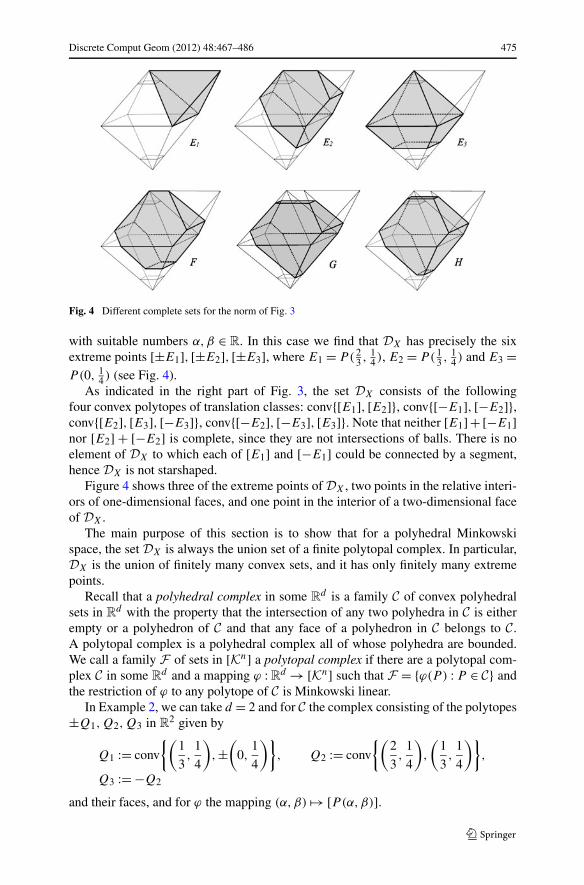
Fig. 4 Different complete sets for the norm of Fig. 3
with suitable numbers α,β ∈ R. In this case we find that DX has precisely the sixextreme points [±E1], [±E2], [±E3], where E1 = P( 2
3 , 14 ), E2 = P( 1
3 , 14 ) and E3 =
P(0, 14 ) (see Fig. 4).
As indicated in the right part of Fig. 3, the set DX consists of the followingfour convex polytopes of translation classes: conv{[E1], [E2]}, conv{[−E1], [−E2]},conv{[E2], [E3], [−E3]}, conv{[−E2], [−E3], [E3]}. Note that neither [E1]+ [−E1]nor [E2] + [−E2] is complete, since they are not intersections of balls. There is noelement of DX to which each of [E1] and [−E1] could be connected by a segment,hence DX is not starshaped.
Figure 4 shows three of the extreme points of DX , two points in the relative interi-ors of one-dimensional faces, and one point in the interior of a two-dimensional faceof DX .
The main purpose of this section is to show that for a polyhedral Minkowskispace, the set DX is always the union set of a finite polytopal complex. In particular,DX is the union of finitely many convex sets, and it has only finitely many extremepoints.
Recall that a polyhedral complex in some Rd is a family C of convex polyhedral
sets in Rd with the property that the intersection of any two polyhedra in C is either
empty or a polyhedron of C and that any face of a polyhedron in C belongs to C .A polytopal complex is a polyhedral complex all of whose polyhedra are bounded.We call a family F of sets in [Kn] a polytopal complex if there are a polytopal com-plex C in some R
d and a mapping ϕ : Rd → [Kn] such that F = {ϕ(P ) : P ∈ C} and
the restriction of ϕ to any polytope of C is Minkowski linear.In Example 2, we can take d = 2 and for C the complex consisting of the polytopes
±Q1,Q2,Q3 in R2 given by
Q1 := conv
{(1
3,
1
4
),±
(0,
1
4
)}, Q2 := conv
{(2
3,
1
4
),
(1
3,
1
4
)},
Q3 := −Q2
and their faces, and for ϕ the mapping (α,β) �→ [P(α,β)].
476 Discrete Comput Geom (2012) 48:467–486
Theorem 3 If X is a polyhedral Minkowski space, then DX is the union set of a finitepolytopal complex.
The proof of the theorem requires a number of preparations. As already men-tioned, it is convenient to use the standard Euclidean scalar product 〈·, ·〉 as an aux-iliary tool. This allows us to use Euclidean normal vectors of hyperplanes and, later,to employ the support function hK of K ∈ Kn, as a function on R
n. In particular, aclosed halfspace can be written in the form
H−(u, η) := {x ∈ R
n : 〈x,u〉 ≤ η}
with u ∈ Rn \ {o} and η ∈ R.
We shall deduce Theorem 3 from a result of McMullen [10], which is based onthe technique of diagrams and representations of polyhedra. We refer to [10] for thistechnique, but we must explain McMullen’s approach with the necessary details thatwe need to apply his result.
Let ±u1, . . . ,±uN be the outer unit normal vectors of the facets of the unit ball B .We write U for the k-tuple (u1, . . . , uk), k = 2N , with ui+N := −ui for i = 1, . . . ,N .Let σ be a representation associated with U , that is, a linear mapping from R
k intoR
k−n with kernel
kerσ = {(〈b,u1〉, . . . , 〈b,uk〉) : b ∈ R
n}. (3)
We refer to [10] for the construction of such a mapping by means of a ‘linear rep-resentation’. If (e1, . . . , ek) is the standard basis of R
k , we define ui := σ(ei) fori = 1, . . . , k and denote by U the k-tuple (u1, . . . , uk). The k-tuple U is called arepresentation of U .
For given (η1, . . . , ηk) ∈ Rk , the set
P :=k⋂
i=1
H−(ui, ηi) (4)
is either empty or a polytope whose facets have only normal vectors from {u1, . . . , uk}.The set of all polytopes of the form (4) is denoted by P (U). If P �= ∅, the point
p = σ(η1, . . . , ηk) =k∑
i=1
ηiui
is said to be associated with P . In virtue of (3), the point p is associated preciselywith the polytopes of the translation class [P].
The following results are proved in [10]. Let P ∈ P (U). Then p ∈ posU , andintP �= ∅ if and only if p ∈ int posU . The vector ui is the normal vector of somefacet of P if and only if p ∈ int pos (U \ {ui}).
For a given P ∈ P (U), the numbers ηi in (4) are in general not uniquely deter-mined by P , but we can always assume that
ηi = ηi(P ) := h(P,ui) (5)
for i = 1, . . . , k; here h(P, ·) is the support function of P . The point p(P ) =∑ki=1 h(P,ui)ui is called the representative of P . All translates of P have the same
Discrete Comput Geom (2012) 48:467–486 477
representative. A point p associated with P is its representative if and only if it be-longs to the closed inner region, which is defined by
clirU :=k⋂
j=1
pos(U \ {uj }
).
The continuous, surjective mapping
�: P (U) → clirU, P �→ p(P ),
which associates with each polytope of P (U) its representative, has the property that�−1(p) ∈ PT (U) for p ∈ clirU , where PT (U) (using McMullen’s notation) denotesthe set of translation classes of polytopes from P (U) (as a subspace of [Kn], hencewith the quotient topology).
As defined by McMullen [10], a type-cone is any subset of clirU which is anonempty intersection of sets of the form relint pos V with V ⊆ U . Thus, clirU ispartitioned into the type-cones. The bijective mapping
�−1: clirU → PT (U)
has the following properties. It is continuous. Restricted to the closure of any type-cone, it is Minkowski linear. And, most important: points p and q of clirU belongto the same type-cone if and only if their images under �−1 are translation classesof strongly isomorphic polytopes. The polytopes P1,P2 are strongly isomorphic (see[14, pp. 100 ff]) if
dimF(P1, u) = dimF(P2, u)
for all vectors u �= o; here F(P,u) denotes the support set of P with outer normalvector u. This is an equivalence relation, and the equivalence class of a polytope P iscalled its a-type. (The ‘a’ comes from ‘analogous’, which is used synonymously for‘strongly isomorphic.)
Theorem 6 of [10] characterizes the type-cones as the maximal relatively openconvex subsets of clirU on which �−1 is Minkowski linear. Finally, Theorem 8 of[10] states that the closures of the type-cones in clirU form a polyhedral complex.
Now we proceed to the proof of Theorem 3.
Lemma 5 For each type-cone K, the intersection K ∩ �(D2) is convex.
Proof Let K be a type-cone, and suppose that p,p′ ∈ K ∩ �(D2). Choose polytopesP ∈ �−1(p) and P ′ ∈ �−1(p′). Then
p =k∑
i=1
h(P,ui)ui, p′ =k∑
i=1
h(P ′, ui
)ui.
Let λ ∈ [0,1] and put Q := (1 − λ)P + λP ′. Then q = (1 − λ)p + λp′ is therepresentative of Q.
We may assume, after renumbering, that ±u1, . . . ,±um (for some m ≤ N )are precisely the normal vectors of the P -regular supporting slabs of P . Recallthat the supporting slab of P with normal vector u is P -regular if and only if
478 Discrete Comput Geom (2012) 48:467–486
max{dimF(P,u),dimF(P,−u)} = n − 1. Since p and q lie in the same type-cone K, the polytopes P and Q are strongly isomorphic, hence
dimF(Q,ui) = dimF(P,ui),
for i = 1, . . . , k. Therefore, ±u1, . . . ,±up are precisely the normal vectors of theQ-regular supporting slabs of Q and, of course, also of P ′.
Since p,p′ ∈ �(D2), the polytopes P,P ′ are complete and have diameter 2.Therefore, Lemma 1 gives
h(P,ui) + h(P,−ui) ≤ 2h(B,ui), h(P ′, ui
) + h(P ′,−ui
) ≤ 2h(B,ui)(6)
for i = 1, . . . ,N and
h(P,ui) + h(P,−ui) = 2h(B,ui), h(P ′, ui
) + h(P ′,−ui
) = 2h(B,ui)(7)
for i = 1, . . . ,m. From (6) and (7) it follows that
h(Q,ui) + h(Q,−ui) ≤ 2h(B,ui) for i = 1, . . . ,N,
h(Q,ui) + h(Q,−ui) = 2h(B,ui) for i = 1, . . . ,m.
We conclude that each B-regular supporting slab of Q has width at most 2 and thateach Q-regular supporting slab of Q has width 2. By Lemma 1, Q has diameter 2and is complete. Therefore, q ∈ �(D2). Thus, K ∩ �(D2) is convex. �
Let i ∈ {1, . . . ,N}. The set
Hi := {(η1, . . . , ηk) ∈ R
k : ηi + ηi+N = 2h(B,ui)}
is a hyperplane. Therefore, the set σ(Hi) is a hyperplane in Rk−n (it is not the whole
space, since Hi ∩kerσ = ∅). Let S+i , S−
i ⊂ Rk−n be the two open halfspaces bounded
by σ(Hi). Calling two points of Rk−n equivalent if they belong to the same elements
of σ(H1), . . . , σ (HN),S+1 , S−
1 , . . . , S+N,S−
N , we obtain a partition of Rk−n into the
equivalence classes. They are relatively open convex polyhedral sets and are calledthe cells. By a type-cell we understand any nonempty intersection of a type-cone and acell. Since the closures of the type-cones form a polyhedral complex, by McMullen’sresult, and clearly also the closures of the cells form a polyhedral complex, we deducethat the closures of all type-cells form a polyhedral complex.
Lemma 6 Let T be a type-cell, and suppose that C := T ∩ �(D2) contains morethan one point. Then
relbdC ⊂ relbdT .
Proof By Lemma 5, the set C is convex. Suppose, contrary to the assertion, that thereexists a point p ∈ relbdC with p ∈ relintT . Since C contains more than one point,we can choose a point p′ ∈ relintC with p′ �= p. We can further choose a numberε > 0 such that qε := p + ε(p − p′) ∈ T , which is possible since p ∈ relintT and
Discrete Comput Geom (2012) 48:467–486 479
p′ ∈ T . Let P ∈ �−1(p), P ′ ∈ �−1(p′) and Qε ∈ �−1(qε). Since p,p′, qε ∈ clirU ,we have
p =k∑
i=1
h(P,ui)ui, p′ =k∑
i=1
h(P ′, ui
)ui, qε =
k∑
i=1
h(Qε,ui)ui,
hencek∑
i=1
[ηi − h(Qε,ui)
]ui = o with ηi := (1 + ε)h(P,ui) − εh
(P ′, ui
).
This implies(η1 − h(Qε,u1), . . . , ηk − h(Qε,uk)
) ∈ kerσ.
Therefore, there exists a vector b ∈ Rn with
ηi − h(Qε,ui) = 〈b,ui〉 for i = 1, . . . , k,
which means that
h(Qε + b,ui) = (1 + ε)h(P,ui) − εh(P ′, ui
), i = 1, . . . , k. (8)
Since P,P ′,Qε belong to the same type-cell, they belong to the same type-coneand hence are strongly isomorphic. As in the proof of Lemma 5, we may assume, afterrenumbering, that ±u1, . . . ,±um are precisely the normal vectors of the P -regularsupporting slabs of P ; then ±u1, . . . ,±um have the same meaning for P ′ and Qε .Since p,p′ ∈ �(D2), relations (6) and (7) are valid, and we deduce from (8) that
h(Qε,ui) + h(Qε,−ui) = 2h(B,ui) for i = 1, . . . ,m.
Suppose that for some j > m we have
h(Qε,uj ) + h(Qε,−uj ) > 2h(B,uj ).
We have P ∈ D2 and hence h(P,uj ) + h(P,−uj ) ≤ 2h(B,uj ). If equality holdshere, then p ∈ σ(Hj ). Since p,qε ∈ T , the points p and qε are in the same type-cell and hence belong to the same of the hyperplanes σ(H1), . . . , σ (HN), in partic-ular qε ∈ σ(Hj ), which implies that h(Qε,uj ) + h(Qε,−uj ) = 2h(B,uj ), a con-tradiction. Therefore, h(P,uj ) + h(P,−uj ) < 2h(B,uj ). By continuity, there ex-ists ε′ with 0 ≤ ε′ ≤ ε and h(Qε′ , uj ) + h(Qε′ ,−uj ) = 2h(B,uj ). This means thatqε′ ∈ σ(Hj ), again a contradiction, for the same reason. Thus, the assumption wasfalse, and we have h(Qε,uj )+h(Qε,−uj ) ≤ 2h(B,uj ) for j = 1, . . . , k. This com-pletes the proof of the fact that Qε ∈ D2 and hence qε ∈ �(D2). From qε ∈ C andp′ ∈ relintC and the convexity of C it now follows that p ∈ relintC, a contradiction.This completes the proof of Lemma 6. �
By Lemma 6, the following holds. If T ∩ �(D2) �= ∅ for some type-cell T , then
T ∩ �(D2) = aff(T ∩ �(D2)
) ∩ T .
It is now easy to see that the closures of the nonempty intersections T ∩�(D2), whereT is a type-cell, form a polyhedral complex. It is, in fact, a polytopal complex, sinceDX is compact and the inverse of the mapping �−1 is continuous. Since the mapping�−1 is Minkowski linear on each type-cone, and thus on each type-cell intersectedwith �(D2), we have proved Theorem 3.
480 Discrete Comput Geom (2012) 48:467–486
5 Extreme Points
In order to gather some more information about the space DX , we study its extremepoints. First, we give an example in which any neighborhood of [B] in DX containsconvex subsets of a given finite dimension, but [B] itself is an extreme point.
The example is the space X = (Rn,‖ · ‖), where the unit ball B of the norm isa polyhedral spindle, that is, a polytope with a vertex p such that each facet of B
contains either p or −p. Let u1, . . . , uN be the outer unit normal vectors of the facetsof B containing p, then −u1, . . . ,−uN are the normal vectors of the facets containingq := −p. Suppose that
B = (1 − λ)K0 + λK1 with K0,K1 ∈ D2, 0 < λ < 1. (9)
For any vector v �= o with F(B,v) = {p} it follows from (9) that F(K0, v) = {p0},F(K1, v) = {p1} with p0 ∈ K0, p1 ∈ K1 and p = (1 − λ)p0 + λp1. Similarly,F(K0,−v) = {q0}, F(K1,−v) = {q1} with q0 ∈ K0, q1 ∈ K1 and q = (1 − λ)q0 +λq1. For i = 1, . . . ,N we have
hence 〈p0, ui〉 = h(K0, ui) and thus p0 ∈ F(K0, ui), similarly q0 ∈ F(K0,−ui).Since K0,K1 ∈ D2, the Minkowski width w satisfies w(K0, ui) ≤ 2, w(K1, ui) ≤ 2.From (9) we get
2 = w(B,ui) = (1 − λ)w(K0, ui) + λw(K1, ui) ≤ 2
and hence w(K0, ui) = 2. Therefore, 〈p0, ui〉 + 〈q0,−ui〉 = 2〈p,ui〉, which gives
〈p,ui〉 = 〈p0, ui〉 −⟨
1
2(p0 + q0), ui
⟩, 〈q,ui〉 = 〈q0, ui〉 −
⟨1
2(p0 + q0), ui
⟩.
Since
B =N⋂
i=1
[H−(
ui, 〈p,ui〉) ∩ H−(−ui, 〈q,−ui〉
)],
K0 =N⋂
i=1
[H−(
ui, 〈p0, ui〉) ∩ H−(−ui, 〈q0,−ui〉
)],
we now deduce that B = K0 − 12 (p0 + q0). Similarly, K1 is a translate of B . This
shows that [B] is an extreme point of DX .To show the second announced property of this example, let Σi denote the B-
regular supporting slab of B with normal vectors ±ui , i = 1, . . . ,N . We assume,without loss of generality, that uN−n+1, . . . , uN are linearly independent and considerthe polytopes
P(α1, . . . , αN−n) :=N−n⋂
i=1
(Σi + αiui) ∩n⋂
j=1
ΣN−n+j .
Discrete Comput Geom (2012) 48:467–486 481
There is a neighborhood U of (0, . . . ,0) ∈ RN−n such that for (α1, . . . , αN−n) ∈ U
the polytope P(α1, . . . , αN−n) has the same number of facets as B and belongs to D2.Further, we can find (α0
1, . . . , α0N−n) ∈ U such that the polytope P(α0
1, . . . , α0N−n) is
simple. By Lemma 2.4.12 of [14], there exists a neighborhood V of (α01, . . . , α0
N−n)
in U such that for (α1, . . . , αN−n) ∈ V the polytopes P(α1, . . . , αN−n) belong to thesame equivalence class of strongly isomorphic polytopes. If P1, . . . ,Pk are stronglyisomorphic polytopes in D2, then the polytope λ1P1 + · · · + λkPk (λ1, . . . , λk ≥ 0,λ1 + · · · + λk = 1) belongs to D2 (as used in the proofs of Lemmas 5 and 6). Weconclude that there is an (N − n)-dimensional convex subset C of V such that for(α1, . . . , αN−n) ∈ C the polytopes P(α1, . . . , αN−n) belong to D2. It follows that anyneighborhood of [B] in DX contains a convex subset of dimension N − n.
As mentioned, Theorem 3 implies that for a polyhedral Minkowski space X, theset DX has only finitely many extreme points. One may conjecture that polyhe-dral Minkowski spaces are characterized by this fact, but we have only been ableto prove this in the two-dimensional case. In higher dimensions, we can show thatin Minkowski spaces with a strictly convex norm, the set DX has infinitely manyextreme points. This requires to deal with two tasks: to construct extreme completesets of given diameter, and for different ones to show that they are not equivalent bytranslation. First we consider strictly convex norms.
Lemma 7 Let X be a Minkowski space with a strictly convex norm. Let ∅ �= S ⊂ X
be a set of vectors of norm 2 with diamS ≤ 2, and let C be a completion of minimalvolume of So := S ∪ {o}. Then [C] is an extreme element of DX .
Proof Since the set γ (So) of completions of So is compact, it is clear that a com-pletion C ∈ γ (So) of minimal volume exists. We assert that C is extreme, in the setof complete sets of diameter 2 (notice that diamC = diamSo = 2). For the proof, letK,M ⊂ X be two complete sets of diameter 2 such that
C = (1 − λ)K + λM (10)
for some λ ∈ (0,1). For x ∈ So, there exist points xK ∈ K and xM ∈ M such that x =(1 − λ)xK + λxM . We assume, without loss of generality, that oK = oM = o, sincethis can be achieved by applying suitable translations to K and M without destroyingthe relation (10). From diamK = diamM = 2 it then follows that ‖xK‖ ≤ 2 and‖xM‖ ≤ 2. For x ∈ S we obtain
2 = ‖x‖ = ∥∥(1 − λ)xK + λxM
∥∥ ≤ (1 − λ)‖xK‖ + λ‖xM‖ ≤ 2.
Since equality holds and the norm is strictly convex, we deduce that xK = xM = x.Thus, So ⊂ K and So ⊂ M , therefore K and M are completions of So. Since C is aminimum volume completion of So, the volumes of K,M,C satisfy V (K) ≥ V (C),V (M) ≥ V (C). From (10) and the Brunn–Minkowski theorem it follows that
V (C)1/n ≥ (1 − λ)V (K)1/n + λV (M)1/n ≥ V (C)1/n.
Since equality holds here, the bodies K and M are homothetic and hence, havingthe same diameter, are translates of each other. This entails that [C] is an extremeelement of DX . �
482 Discrete Comput Geom (2012) 48:467–486
The proof of Lemma 7 leads us to the following side-remark on the so-calledMeissner bodies in Euclidean three-space 3
2. To obtain them, one starts with a regu-lar tetrahedron T of edge length d , forms the intersection of the balls of radius d withcenters at the vertices of T , and then rounds off one edge from each opposite pairof curved edges to obtain a body of constant width d . These bodies were introducedby Meissner [11], their construction is described in Bonnesen–Fenchel [1, p. 136]; aphotograph of a plaster model can be found in Fischer [4, p. 98]. They are famousdue to the fact that they have been conjectured (Bonnesen–Fenchel, loc. cit.) to be thebodies of constant width d of minimal volume; this is still undecided. The problem,its history and some recent developments are neatly presented in the article by Ka-wohl and Weber [8]. The conjecture would be disproved if it could be shown that aMeissner body does not define an extreme class in D3
2; however, this approach fails.
Proposition 1 The translation class of a Meissner body is extreme in D32.
Proof We make use of the following easily proved facts. (i) If C is a subset of diam-eter d in a normed space with unit ball B and if there is a subset C′ ⊂ C satisfying
diam⋂
t∈C′(dB + t) = d,
then D := ⋂t∈C′(dB + t) is the only completion of C; (ii) If A = conv{a1, a2},
B = conv{b1, b2}, C = conv{c1, c2} are segments in a strictly convex normed spacesatisfying ‖a1 − a2‖ ≥ ‖b1 − b2‖,‖c1 − c2‖ and ai = λbi + (1 − λ)ci , i = 1,2, forsome λ ∈ (0,1), then B and C are translates of A.
There are two types of Meissner body, according to which three curved edgeshave been rounded: three that have a common vertex or three that form a triangle.First we consider the case of a common vertex. Let B be the unit ball of 3
2. Withoutloss of generality, we take the plane H := {(x1, x2, x3) ∈ R
3 : x3 = −2√
2/3} and let{a1, a2, a3} ∈ H ∩∂2B be three points forming with o an equilateral set of diameter 2.If we consider the sets
M0 := (2B + a1) ∩ (2B + a2) ∩ (2B + a3) ∩ ∂2B
and
M1 :=⋂
t∈M0
(2B + t),
then M1 is a Meissner body with the rounded edges having o as common vertex.Moreover, M1 is the only completion of M0 and hence, by Lemma 7, the translationclass [M1] is an extreme element of D3
2.
In order to deal with the second type of Meissner body, consider the halfspaceH+ := {(x1, x2, x3) ∈ R
3 : x3 ≥ −2√
2/3} and define the new sets
M ′0 := (2B + a1) ∩ (2B + a2) ∩ (2B + a3) ∩ H+
and
M ′1 :=
⋂
t∈M ′0
(2B + t).
Discrete Comput Geom (2012) 48:467–486 483
Then M ′1 is the only completion of M ′
0 and is a Meissner body of the second type,with the rounded edges forming a triangle. We state that M ′
1 is extreme, up to trans-lations, in the family of complete sets of diameter 2. In fact, suppose that M ′
1 is aconvex combination of complete sets A and B of diameter 2. Then these two setscontain translates of M ′
0 (as follows from fact (ii) above), which implies that [M ′1] =
[A] = [B]. �
After this digression, we return to the extreme points of DX in general.
Theorem 4 Let X be a Minkowski space with a strictly convex norm. Then the set DX
has continuum many extreme points.
Proof In the following proof, the notions of unit normal vector and spherical imagerefer again to an auxiliary Euclidean metric on X.
Let H be a two-dimensional plane through o and let J := H ∩ ∂2B , where B isthe unit ball of X. We choose a point x1 ∈ J and let y1 be one of the two pointsin J ∩ (J + x1). Then ‖x1 − y1‖ = 2 (this is the known argument to construct anequilateral triangle in a Minkowski plane; see Thompson [15, Theorem 4.1.1]). Letz �= x1, y1 be a point of the arc of J between x1 and y1. Then ‖z − x1‖ < 2 and‖z − y1‖ < 2. Let x2 be a point of the open arc of J between x1 and z, and determiney2 ∈ J such that ‖y2 − x2‖ = 2 and y1 belongs to the open arc of J between z andy2. We can choose x2 so close to x1 that still ‖z − y2‖ < 2; of course, ‖y2 − x1‖ > 2.
There is a neighborhood N of z in X such that ‖w −xi‖ < 2 and ‖w −yi‖ < 2 forall w ∈ N and for i = 1,2. Now we choose n points w1, . . . ,wn ∈ N ∩ ∂2B such thatthere are outer unit normal vectors ui of 2B at wi , i = 1, . . . , n, which are linearlyindependent. That this is possible follows from the fact that 2B is strictly convex. (IfK is a strictly convex body, then the spherical image of a relatively open subset of∂K is a relatively open subset of the unit sphere.)
We define Si := {o, xi, yi,w1, . . . ,wn} for i = 1,2, then diamSi = 2. Let Ci bea minimal volume completion of Si . By Lemma 7, [Ci] is an extreme point of DX .Suppose that C1 and C2 were translates of each other. For j ∈ {1, . . . , n} we haveCi ⊂ 2B + wj , hence o ∈ ∂Ci , and −uj is an outer normal vector to Ci at o. Thepoint o is the only point of Ci at which the normal cone contains the linearly inde-pendent vectors −u1, . . . ,−un. It follows that C1 and C2, which are translates, mustbe identical. But then x1, y2 ∈ Ci , which is a contradiction, since ‖x1 − y2‖ > 2. Thisproves that C1 and C2 are not translates of each other. By varying the points x1 andx2 in suitable neighborhoods, we obtain continuum many different extreme pointsof DX . �
Theorem 5 In a two-dimensional Minkowski space, there are infinitely many extremetranslation classes of bodies of given constant width if and only if the unit ball of thespace is not a polygon.
Proof Recall that in a two-dimensional Minkowski space, the notions of body ofconstant width and of diametrically complete set are equivalent. It follows from The-orem 3 that in a polyhedral Minkowski plane there are only finitely many extreme
484 Discrete Comput Geom (2012) 48:467–486
translation classes of bodies of given constant width. To prove the converse, we mayrestrict ourselves to convex bodies of constant width one. Similarly as in the pre-vious proof, we choose a point x ∈ ∂B (which we call the ‘starting point’) and lety be a point in ∂B ∩ (∂B + x). Then ‖x‖ = ‖y‖ = ‖x − y‖ = 1. We remark that∂B ∩ (∂B +x) contains precisely two points except if ∂B contains a segment parallelto x and of length larger than one. Let
C := B ∩ (B + x) ∩ (B + y).
Of any two parallel supporting lines of C, at least one passes through one of thepoints o, x, y, and it follows that the lines are distance one apart. Thus, C is a body ofconstant width one. The bodies obtained in this way, and their translates, are calledMinkowski Reuleaux triangles (although they can have more than three vertices).
Suppose that
C = (1 − λ)K + λM (11)
for some K,M ∈ K2 of constant width one and for some λ ∈ (0,1). As in the proofof Lemma 7, there are points oK,xK,yK ∈ K and oM,xM,yM ∈ M such that o =(1 − λ)oK + λoM , x = (1 − λ)xK + λxM , y = (1 − λ)yK + λyM . Moreover, sincey ∈ ∂C, we have yK ∈ ∂K , yM ∈ ∂M , and the outer unit normal vectors (with respectto some scalar product) of C at y, of K at yK and of M at yM are the same. Afterapplying suitable translations we may assume that oK = oM = o; then ‖xK‖ ≤ 1,‖yK‖ ≤ 1. In
1 = ‖x‖ = ∥∥(1 − λ)xK + λxM
∥∥ ≤ (1 − λ)‖xK‖ + λ‖xM‖ ≤ 1 (12)
we have equality. Equality in the second inequality yields ‖xK‖ = ‖xM‖ = 1, hencexK,xM ∈ ∂B . Similarly, we obtain ‖yK‖ = ‖yM‖ = 1. Equality in the first inequalityof (12) implies that the segment with endpoints xK,xM lies in the boundary of B .Now we introduce a first additional assumption, namely that x was chosen as anextreme point of B; then we can conclude that xK = xM = x. From
1 = ‖x − y‖ = ∥∥x − (1 − λ)yK − λyM
∥∥ = ∥∥(1 − λ)(x − yK) + λ(x − yM)∥∥
≤ (1 − λ)‖xK − yK‖ + λ‖xM − yM‖ ≤ 1
we obtain ‖x − yK‖ = 1 = ‖x − yM‖. Since also ‖yK‖ = ‖yM‖ = 1, we deduce thatyK,yM ∈ ∂B ∩ (∂B + x). As a second assumption, we assume now that ∂B does notcontain a segment parallel to x and of length larger than one. Then ∂B ∩ (∂B + x)
consists of precisely two points, one of which is y. Since the outer unit normal vectorsof C at y, of K at yK and of M at yM are the same (and o, x ∈ K,M), we concludethat yK = yM = y. Thus, o, x, y ∈ K , and since K is of constant width one, we musthave K ⊂ B ∩ (B + x) ∩ (B + y) = C. In fact, equality must hold here, since anyproper closed convex subset of B ∩ (B + x) ∩ (B + y) is not of constant width one.Similarly, we have M = C. Thus, C is extreme.
Now we assume that the unit ball B of X is not a polygon; then it has infinitelymany extreme points. We say that an extreme point x is suitable if ∂B does notcontain a segment of length at least one that is parallel to x. Clearly, at most finitelymany of the extreme points are not suitable. Let x0 be an accumulation point ofextreme points. There is a point z ∈ ∂B ∩ int(B + x0) such the arc of ∂B between x0
Discrete Comput Geom (2012) 48:467–486 485
and z contains infinitely many extreme points. We choose a cyclic order on ∂B , andwe take two different suitable extreme points x1 and x2 from the open arc betweenx0 and z such that x0, x1, x2, z follow each other in cyclic order. We choose y1 as thefirst point in ∂B ∩ (∂B + x1) after z in cyclic order, and y2 is defined similarly, forthe starting point x2. Let Ci be the completion of {o, xi, yi}, i = 1,2, as constructedabove, with starting point xi . As shown, C1 and C2 are extreme bodies of constantwidth one. Suppose that C2 is a translate of C1, say C2 + t = C1 with t ∈ R
2. Clearly,t �= o. Since x2 + t ∈ C2 + t = C1 ⊂ B and x2 − t ∈ C1 − t = C2 ⊂ B , the pointx2 is not an extreme point of B , which is a contradiction. Thus, C1 and C2 are nottranslates of each other. It follows that there are infinitely many translation classes ofextreme bodies of constant width one. �
Example 3 The following example shows that Minkowski Reuleaux triangles arenot always extreme. Let the unit ball B of X be an affinely regular hexagon, withvertices v1, v2, v3,−v1,−v2,−v3, in cyclic order. Performing the construction of theprevious proof with the starting point x1 = v1, we obtain a Minkowski Reuleauxtriangle C1 which is an ordinary triangle. Starting with x2 = v2, we get a differentMinkowski Reuleaux triangle C2, which is also an ordinary triangle. The hexagonC := 1
2 (C1 + C2) is the Minkowski Reuleaux triangle which is obtained when westart with the (non-extreme) point 1
2 (x1 + x2). Thus, C is a non-extreme MinkowskiReuleaux triangle.
Remark Kallay [7] has proved a necessary and sufficient condition for a convex bodyof constant width in a two-dimensional Minkowski space to be extreme in the set ofall convex bodies of the same constant width. We found the proof given above moredirect than an application of this criterion. (Note also that in [7, Theorem 2], thecondition θ ∈ [0,2π) has to be replaced by θ ∈ [0,π), as shown by the example ofthe space 2∞, and also by the proof given in [7].)
References
1. Bonnesen, T., Fenchel, W.: Theorie der konvexen Körper. Springer, Berlin (1934). English translation:L. Boron, C. Christenson, B. Smith (eds.) Theory of Convex Bodies. BCS Associates, Moscow, ID(1987)
2. Chakerian, G.D., Groemer, H.: Convex bodies of constant width. In: Gruber, P.M., Wills, J.M. (eds.)Convexity and Its Applications, pp. 49–96. Birkhäuser, Basel (1983)
3. Eggleston, H.G.: Sets of constant width in finite dimensional Banach spaces. Isr. J. Math. 3, 163–172(1965)
4. Fischer, G.: Mathematische Modelle. Mathematical Models. Vieweg, Braunschweig (1986)5. Groemer, H.: On complete convex bodies. Geom. Dedic. 20, 319–334 (1986)6. Heil, E., Martini, H.: Special convex bodies. In: Gruber, P.M., Wills, J.M. (eds.) Handbook of Convex
Geometry, pp. 347–385. North-Holland, Amsterdam (1993)7. Kallay, M.: The extreme bodies in the set of plane convex bodies with a given width function. Isr. J.
Math. 22, 203–207 (1975)8. Kawohl, B., Weber, C.: Meissner’s mysterious bodies. Math. Intell. 33, 94–101 (2011)9. Martini, H., Swanepoel, K.J.: The geometry of Minkowski spaces—a survey. Part II. Expo. Math. 22,
93–144 (2004)10. McMullen, P.: Representations of polytopes and polyhedral sets. Geom. Dedic. 2, 83–99 (1973)
486 Discrete Comput Geom (2012) 48:467–486
11. Meissner, E., Schilling, F.: Drei Gipsmodelle von Flächen konstanter Breite. Z. Math. Phys. 60, 92–94(1912)
12. Moreno, J.P., Schneider, R.: Local Lipschitz continuity of the diametric completion mapping. Houst.J. Math., in press
13. Moreno, J.P., Schneider, R.: Diametrically complete sets in Minkowski spaces. Isr. J. Math. (2012).doi:10.1007/s11856-012-0003-6
14. Schneider, R.: Convex Bodies: The Brunn–Minkowski Theory. Cambridge University Press, Cam-bridge (1993)
15. Thompson, A.C.: Minkowski Geometry. Cambridge University Press, Cambridge (1996)