Study of Beam Loss Monitors (BLM) in Storage Ring

S. M. Esmaeilic, S. A. H. Feghhic cRadiation Applications Department, Shahid Beheshti University,Evin, G. C. Tehran, Iran

ABSTRACT: The Beam Loss Monitors (BLM) are designed to measure the position and amount

of beam loss in accelerators. In this article, we have studied the 3 GeV electron losses in the

storage ring and secondary particles from the losses on the beam pipe. We have compared

ionization chamber, NaI and Si radiation detectors as BLM and selected Si detector for further

studies. We have calculated electron deflection angle due to magnetic field mismatches in dipole

magnets, quadrupoles and sextupoles and assumed that electron beam is deflected and hit the

beam pipe with the angle of 3 degrees with respect to the beam axis. The number and energy of

photons and secondary particles on beam pipe and in Si detector are calculated by the MCNP code

and reported in this paper.

KEYWORDS: Beam Loss Monitors; Storage Ring; Secondary Particles; Particle Detectors.

– 1 –

1. Introduction

With the information provided by the BLM placed around the storage ring, beam loss distribution

pattern can be directly monitored [1]. We can use beam loss distribution pattern to improve the

performance of storage ring in terms of life time and stability [1]. Beam losses can be caused by

collision of the beam to the diagnostics equipment such as Faraday cups, wire scanners, scrapers

or any other devices which are located on the beam path or by other reasons such as residual gas

scattering, misalignment, instabilities, and Halo scraping [2][3][4][5].

In this paper, we have studied the losses due to the magnet misalignment, magnet vibration and

magnet current fluctuations that causes the beam to experience different magnetic fields [6].

We have calculated the deflection angle of electron beam due to the magnetic field mismatches

in dipole, quadrupoles and sextuples magnets geometrically to be around 0.5 to 6 degrees. In the

following calculations we have considered the electron typical deflection angle of 3 degrees.

We have calculated the number and energy of secondary particles generated from hitting of the

deflected 3GeV electrons to the storage ring beam pipe via MCNP code [7]. In all calculations

typical storage ring’s parameters are considered [8][9][10][11]. According to the simulation

results, 34.8 electrons, 139.7 photons and 0.1 neutrons are exited from the beam pipe with the

total energy of 1073.3 MeV, 1467.9 MeV and 1.3 MeV, respectively.

To detect such losses, beam position monitors are one of the essential sensors, but their

information is not sufficient, that is why we need other types of radiation detectors around the

storage ring [12][13][14][15][16]. Radiation detectors such as scintillators or silicon detectors are

found in variety of applications such astronomy, nuclear physics, medicine and even air pollutions

[17][18][19][20][21][22].

In the following we study ionization chamber, NaI and Si detectors as beam loss monitors. Among

them, Si detector is selected in our studies due to its advantages of high resolution, high efficiency,

linear response in a wide range of energy, relatively fast response, being not sensitive to the

magnetic field, and possibility to construct in various forms [23]. The Si detector is placed 10 cm

away from the beam pipe and the number and energy of photons and secondary particles that

would reach the detector are calculated by MCNP code [7]. It is concluded that only 0.05

electrons, 0.9 photons and 0.57 neutrons with the total deposited energy of 0.16 MeV, 3.89 MeV

and 0.003 MeV respectively will reach the detector.

2. Loss Angle

The angle of loss is the angle with respect to the beam axis at which the electron particle is

separated from the beam and collides with the accelerator beam pipe. This angle is essential for

calculation of the secondary particle characteristics. Beam loss may occur as a result of magnet

vibrations, electrical current fluctuations in magnets winding or magnet misalignment [24]. These

factors make electrons to experience a different magnetic field than the optimal and normal value

when they pass through magnets. So, if the magnetic field applied to the particles are less or more

than nominal, particles do not travel their pre-defined path, and may hit the beam tube and become

lost. Therefore, by changing the values of magnetic field, the loss angle could be obtained.

– 2 –

2.1. Loss angle due to dipole magnet mismatch

In order to obtain the loss angle and the collision point of electron on the beam tube, it is assumed

that the dipole magnet’s magnetic field to be less or greater than its nominal value of 0.748 T in

the storage ring [8]. By changing the magnetic field value, electrons travel circular paths with

smaller or larger radii and collide to the beam pipe and become lost.

In the our storage ring study case, the bending angle of dipoles is 3.6 degrees, therefore, the total

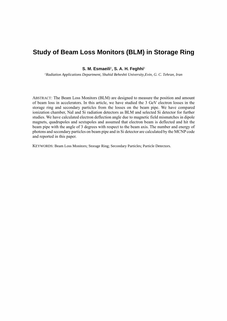
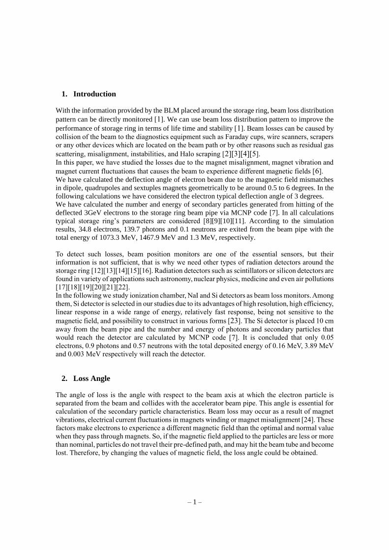
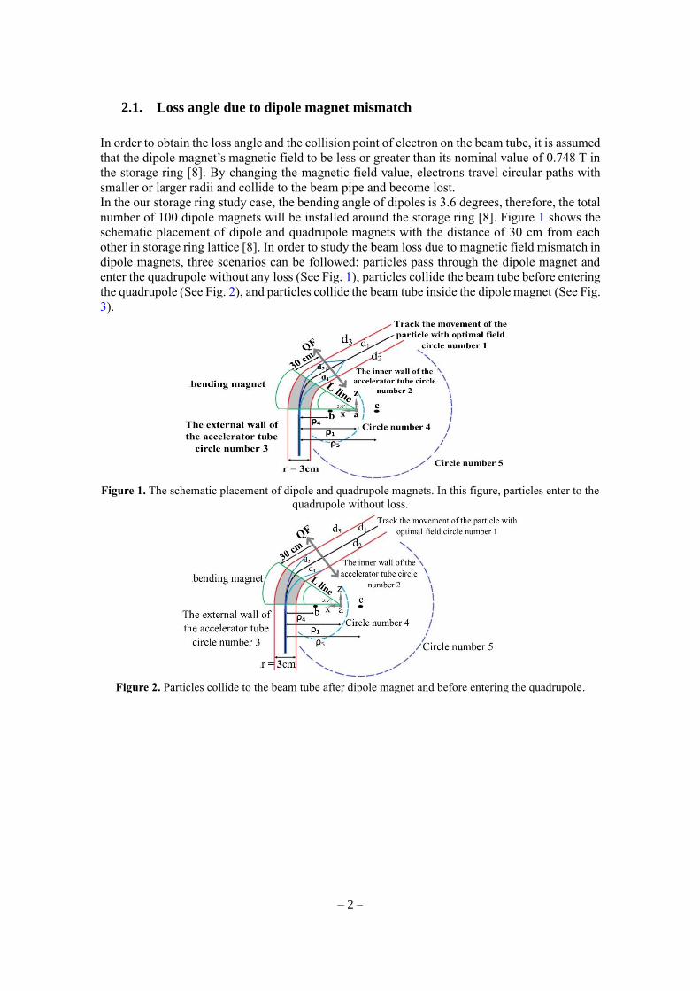
number of 100 dipole magnets will be installed around the storage ring [8]. Figure 1 shows the

schematic placement of dipole and quadrupole magnets with the distance of 30 cm from each

other in storage ring lattice [8]. In order to study the beam loss due to magnetic field mismatch in

dipole magnets, three scenarios can be followed: particles pass through the dipole magnet and

enter the quadrupole without any loss (See Fig. 1), particles collide the beam tube before entering

the quadrupole (See Fig. 2), and particles collide the beam tube inside the dipole magnet (See Fig.

3).

Figure 1. The schematic placement of dipole and quadrupole magnets. In this figure, particles enter to the

quadrupole without loss.

Figure 2. Particles collide to the beam tube after dipole magnet and before entering the quadrupole.

– 3 –

Figure 3. Particles collide to the beam tube inside of dipole magnet.

In these figures, the solid line at the center of beam pipe represents a reference path that particles

should pass through without any disturbance. Inside the dipole magnet particles pass on a circular

path (with the radius of ρ1) and outside of dipoles, they pass on straight lines (d1). The radius of

circular path can be obtained by 𝜌 =𝛾𝑚0𝐶

𝑒𝐵 where 𝛾 is Lorentz factor and m0 is electron rest mass

energy (0.511 MeV), C is speed of light, e is electron charge and B is dipole magnetic field [24].

However, the calculations for superconductive types can be different [25][26][27]. The inner and

outer shells of beam pipe inside the dipole magnet considered as circles with the radiuses of ρ2

and ρ3, respectively, and outside the dipole magnets, they are considered as straight lines d2 and

d3. If the magnetic field of dipole magnet is larger than the nominal value, particles will become

lost because of hitting the inner shell of the beam pipe and will pass the circular path with the

radius of ρ4 inside the magnet and the straight line of d4 outside and if it is lower than the nominal

value, particles will hit the inner shell of the beam pipe and pass the circular path with the radius

of ρ5 inside the magnet and straight line d5 outside. Point “a” is considered as our geometrical

reference point which is the center of circle “1” (See Fig. 1, 2, 3). Line “L” is considered as the

border of dipole magnet where particles travel on a straight line after that. The diameter of beam

pipe is considered to be of 3 cm [28][29].

First, we have calculated the equation of circles “1”, “2”, “3” and lines “d1”, “d2”, “d3” and “L”.

Then for each case of magnetic field, we obtain the equation of circles 4 and 5 in X-Z plane. For

a nominal magnetic field of 0.748 T inside of dipole magnets, ρ1, ρ2, ρ3 are 1338.838 cm, 1337.338

cm and 1340.338 cm respectively. Equation of line “L” is obtained to be x=15.894z. The z

coordinate of intersections between line “L” and circles “2” and “3” are 83.975 cm and 84.163

cm, respectively. Then by calculating the intersection points of line “L” with particle paths (circles

4 and 5) and obtaining their z coordinates, we can conclude that the particles will pass through

the dipole magnets if 83.975 cm<z<84.163 cm, otherwise they are lost inside the magnet (See

Fig. 3).

For these purposes, we have considered the dipole magnets to have magnetic field values between

0.13 T and 1.4 T. Based on our studies, for 0.7481 T ≤ B ≤ 0.99 T and 0.51T ≤ B ≤ 0.7479, particles

will enter the quadrupoles without any loss. For 1 T ≤ B ≤ 1.19 T and 0.33 T ≤ B ≤ 0.5 T, particles

will hit the inner and outer shells of beam pipe at the distance between dipole and quadrupole

magnet. If 1.2 T ≤ B or B ≤ 0.32 T, particles will hit the beam pipe inside the dipole magnet. Table

I shows the calculated deflection angle of electrons for different dipole magnetic field values.

– 4 –

TABLE I. deflection angle of electrons with respect to the reference axis for different dipole magnetic

fields

Magnetic field (T) Deflection angle (Degrees)

1 1.212

0.33 5.189

1.19 2.174

0.5 6.007

1.2 2.108

0.32 2.05

2.2. Loss angle due to quadrupole and sextupole magnets mismatch

The main task of quadrupole magnets is the convergence or divergence of the beam. Defocusing

(QD) and focusing (QF) magnets, converge particle beams in one direction (z axis for QD and x

axis for QF) and diverge them in the other (z axis for QF and x axis for QD) [24]. Due to energy

dispersion, particles with different energies passing through quadrupoles will deflect with

different angles. Higher energy particles are more rigid than lower energy one for the same

magnetic field value. That is why sextupoles are used where particles with higher energy and

lower energy experience higher and lower magnetic fields respectively that makes the

convergence procedure more efficient [30][31].

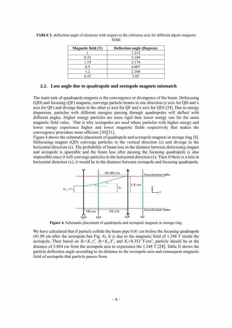
Figure 4 shows the schematic placement of quadrupole and sextupole magnets in storage ring [8].

Defocusing magnet (QD) converge particles in the vertical direction (z) and diverge in the

horizontal direction (x). The probability of beam loss in the distance between defocusing magnet

and sextupole is ignorable and the beam loss after passing the focusing quadrupole is also

impossible since it will converge particles in the horizontal direction (x). Then if there is a loss in

horizontal direction (x), it would be in the distance between sextupole and focusing quadrupole.

Figure 4. Schematic placement of quadrupole and sextupole magnets in storage ring.

We have calculated that if particle collide the beam pipe 0.01 cm before the focusing quadrupole

(41.99 cm after the sextupole-See Fig. 4). It is due to the magnetic field of 1.248 T inside the

sextupole. Then based on Bx=Ks.z2, Bz=Ks.X

2, and Ks=8.352 T/cm2, particle should be at the

distance of 3.864 cm from the sextupole axis to experience the 1.248 T [24]. Table II shows the

particle deflection angle according to its distance to the sextupole axis and consequent magnetic

field of sextupole that particle passes from.

– 5 –

TABLE II. Loss angle and distance between particle collision point and sextupole location

Distance between particle

collision point and sextupole

location (cm)

Loss angle Distance from

sextupole magnet axis

(cm)

Magnetic field (T)

41.99 1.518 0.3866 1.248

38 1.599 0.4386 1.607

34 1.671 0.5076 2.152

30 1.713 0.6024 3.031

27 1.732 0.7005 4.098

According to the calculations, as can be seen in Table I and II, the deflection angle varies based

on the magnetic field from 0.5 to 6 degrees. Angle of deflected electron with respect to the beam

line is one of the main parameters in calculation of secondary particles. Therefore, for calculation

of the number and energy of secondary particles, we assume that the electron beam is deflected

and hit the beam pipe by an angle of 3 degrees.

3. Secondary Particles

We used MCNP code [7] to obtain secondary particle and photon spectrums generated in the

external beam pipe wall due to hitting of the deflected electrons. For this purpose, a hollow

cylinder with the inner and outer radius of 1.5 cm and 1.7 cm is considered the beam pipe. The

length of this cylinder is 4 m, and it is made of stainless steel 316. An electron spot source with

an energy of 3 GeV and deflection angle of 3 degrees is considered at the center of this cylinder.

Figure 5 shows the geometrical parts of our simulation in MCNP [7].

Figure 5. Simulated geometry of the accelerator tube and the BLM detector.

To analyze the secondary particles, as shown in Fig. 5, the 2 mm thickness of steel beam pipe is

divided into equal quadrants of 0.5 mm thickness. As electron penetrates in the steel, it deposits

all its energy in first quadrant and makes secondary particles. Due to 3 degrees deflection angle,

electron passes a distance of 9.56 mm in the first quadrant. In this quadrant, the 1584.03 MeV of

deposited electron energy converts to the photons and secondary electrons where they also stop

in this quadrant and produce more secondary electrons and neutrons, and remaining amount of

deposited energy, 1415.97 MeV, converts to the secondary electrons which exit from this

quadrant. Deposited energy of electrons and photons in the first part is 94.4336 MeV, while this

value is only 0.00349 MeV for neutrons. Therefore, the total deposited energy in the first 0.5 mm

thickness of steel is about 94.43709 MeV.

– 6 –

In the second quadrant, from each 10000 entered secondary electrons, 9993 electrons deposit their

whole energy, so that the amount of 756.998 MeV is converted to secondary electrons and

photons. From each 100000 entered photons from the first quadrant, 65 photons deposit their

whole energy inside second the quadrant, so that the amount of 120.387 MeV is deposited in this

part. From each 10000 entered neutrons from first quadrant, 9986 neutrons deposit their whole

energy in the second quadrant, so that the amount of 0.0025 MeV is deposited in this layer. As a

result, the total energy of 120.3895 MeV is deposited in the second quadrant.

In the third layer, from each 10000 entered secondary electrons, 9910 electrons deposit their

whole energy, so that the amount of 333.084 MeV is converted to secondary electrons and

photons. From each 100000 entered photons from the previous part, 897 photons deposit their

whole energy inside the third layer, so that the total amount of 127.289 MeV is deposited in this

layer. From each 10000 entered neutrons from the second quadrant, 9990 neutrons deposit their

whole energy in the third layer, so that the amount of 0.0033 MeV is deposited in this part. As a

result, the total energy of 127.2923 MeV is deposited in the third quadrant.

In last layer, from each 10000 entered secondary electrons, 9659 electrons deposit their whole

energy, so that the amount of 144.385 MeV is converted to secondary electrons and photons. From

each 100000 entered photons from previous part, 3405 photons deposit their whole energy inside

this layer, so that the amount of 105.610 MeV is deposited in this layer. From each 10000 entered

neutrons from the third quadrant, 9992 neutrons deposit their whole energy, so that the amount of

0.0025 MeV is deposited in this part. As a result, total energy of 105.6125 MeV is deposited in

the fourth layer of steel beam pipe.

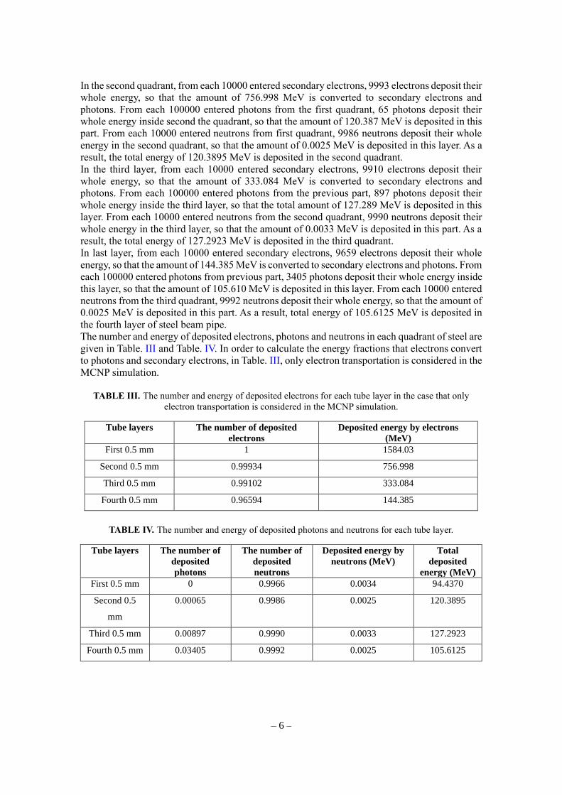
The number and energy of deposited electrons, photons and neutrons in each quadrant of steel are

given in Table. III and Table. IV. In order to calculate the energy fractions that electrons convert

to photons and secondary electrons, in Table. III, only electron transportation is considered in the

MCNP simulation.

TABLE III. The number and energy of deposited electrons for each tube layer in the case that only

electron transportation is considered in the MCNP simulation.

Deposited energy by electrons

(MeV)

The number of deposited

electrons

Tube layers

1584.03 1 First 0.5 mm

756.998 0.99934 Second 0.5 mm

333.084 0.99102 Third 0.5 mm

144.385 0.96594 Fourth 0.5 mm

TABLE IV. The number and energy of deposited photons and neutrons for each tube layer.

Total

deposited

energy (MeV)

Deposited energy by

neutrons (MeV)

The number of

deposited

neutrons

The number of

deposited

photons

Tube layers

94.4370 0.0034 0.9966 0 First 0.5 mm

120.3895 0.0025 0.9986 0.00065 Second 0.5

mm

127.2923 0.0033 0.9990 0.00897 Third 0.5 mm

105.6125 0.0025 0.9992 0.03405 Fourth 0.5 mm

– 7 –

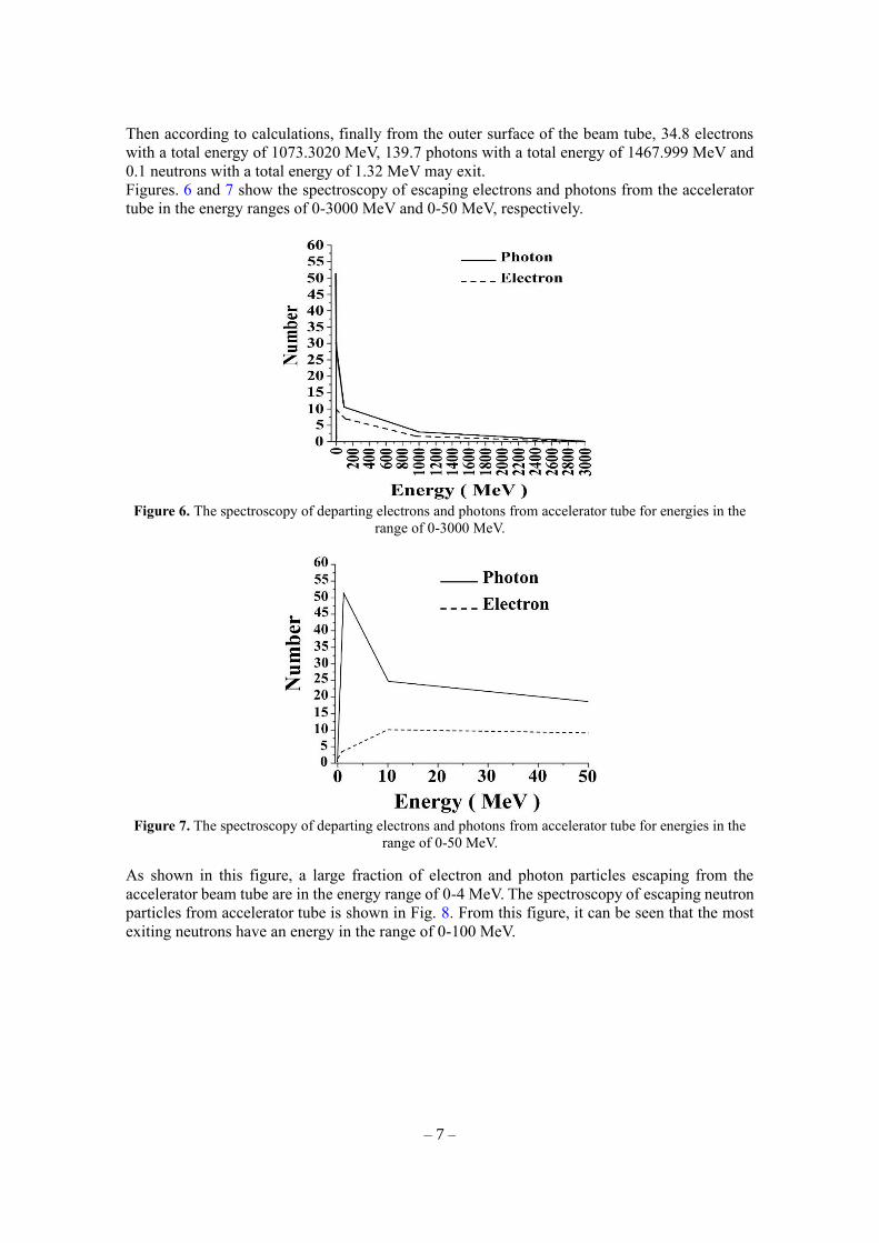
Then according to calculations, finally from the outer surface of the beam tube, 34.8 electrons

with a total energy of 1073.3020 MeV, 139.7 photons with a total energy of 1467.999 MeV and

0.1 neutrons with a total energy of 1.32 MeV may exit.

Figures. 6 and 7 show the spectroscopy of escaping electrons and photons from the accelerator

tube in the energy ranges of 0-3000 MeV and 0-50 MeV, respectively.

Figure 6. The spectroscopy of departing electrons and photons from accelerator tube for energies in the

range of 0-3000 MeV.

Figure 7. The spectroscopy of departing electrons and photons from accelerator tube for energies in the

range of 0-50 MeV.

As shown in this figure, a large fraction of electron and photon particles escaping from the

accelerator beam tube are in the energy range of 0-4 MeV. The spectroscopy of escaping neutron

particles from accelerator tube is shown in Fig. 8. From this figure, it can be seen that the most

exiting neutrons have an energy in the range of 0-100 MeV.

– 8 –

Figure 8. The spectroscopy of neutrons exited from outer shell of beam tube.

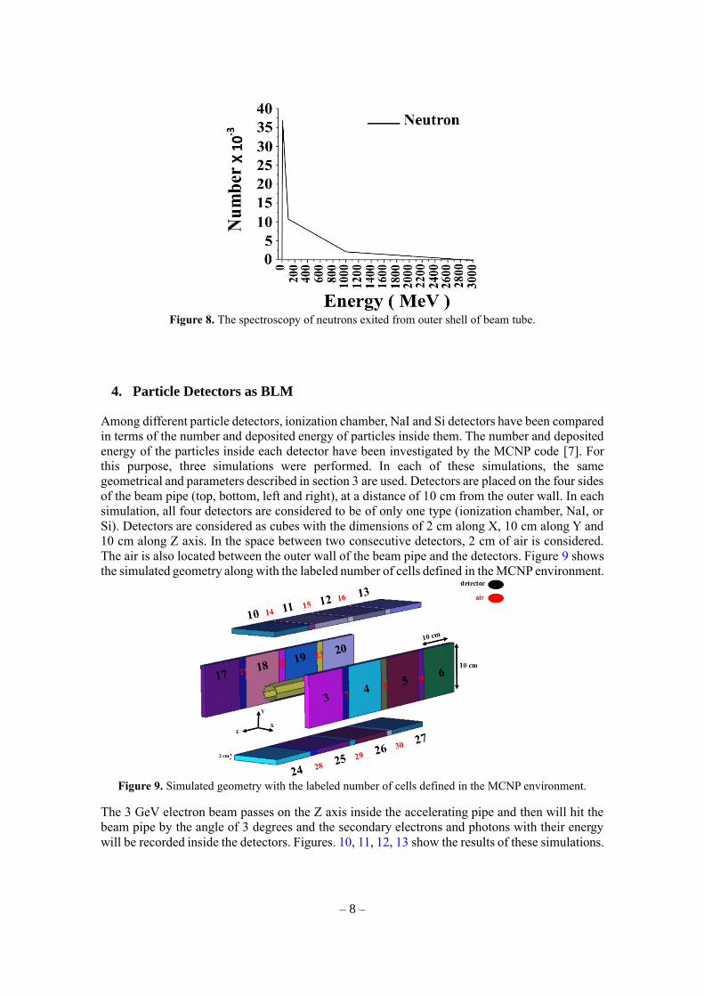
4. Particle Detectors as BLM

Among different particle detectors, ionization chamber, NaI and Si detectors have been compared

in terms of the number and deposited energy of particles inside them. The number and deposited

energy of the particles inside each detector have been investigated by the MCNP code [7]. For

this purpose, three simulations were performed. In each of these simulations, the same

geometrical and parameters described in section 3 are used. Detectors are placed on the four sides

of the beam pipe (top, bottom, left and right), at a distance of 10 cm from the outer wall. In each

simulation, all four detectors are considered to be of only one type (ionization chamber, NaI, or

Si). Detectors are considered as cubes with the dimensions of 2 cm along X, 10 cm along Y and

10 cm along Z axis. In the space between two consecutive detectors, 2 cm of air is considered.

The air is also located between the outer wall of the beam pipe and the detectors. Figure 9 shows

the simulated geometry along with the labeled number of cells defined in the MCNP environment.

Figure 9. Simulated geometry with the labeled number of cells defined in the MCNP environment.

The 3 GeV electron beam passes on the Z axis inside the accelerating pipe and then will hit the

beam pipe by the angle of 3 degrees and the secondary electrons and photons with their energy

will be recorded inside the detectors. Figures. 10, 11, 12, 13 show the results of these simulations.

– 9 –

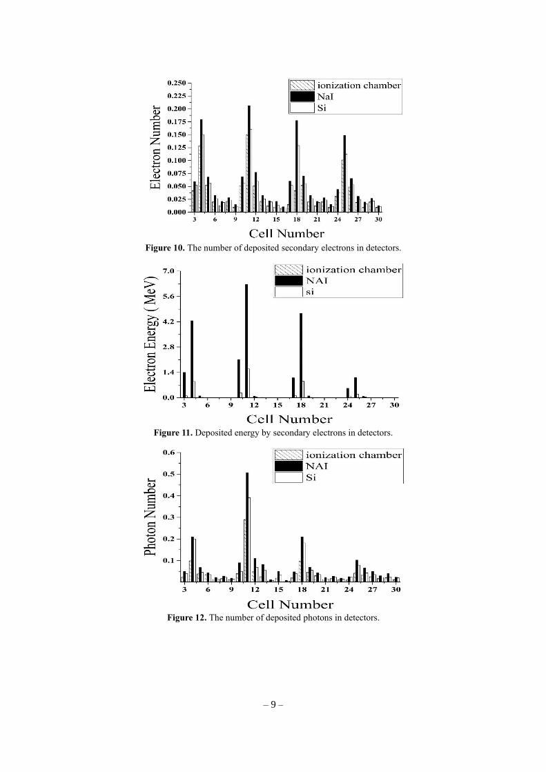
Figure 10. The number of deposited secondary electrons in detectors.

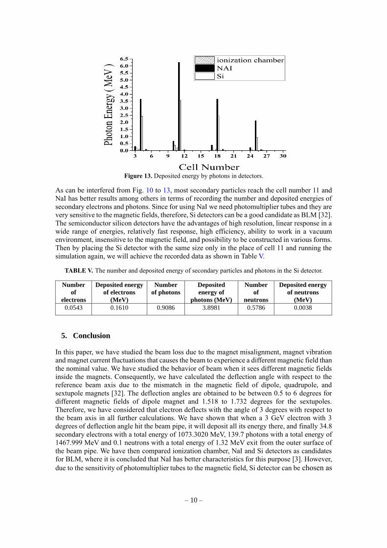
Figure 11. Deposited energy by secondary electrons in detectors.

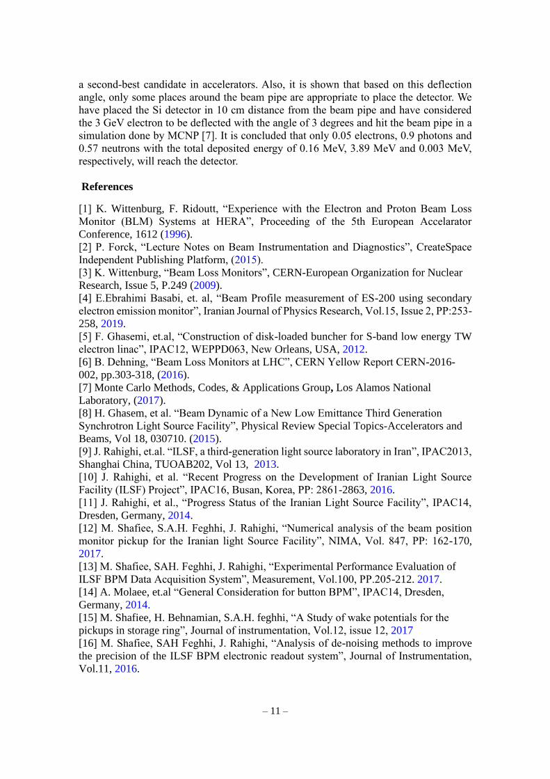
Figure 12. The number of deposited photons in detectors.

– 10 –

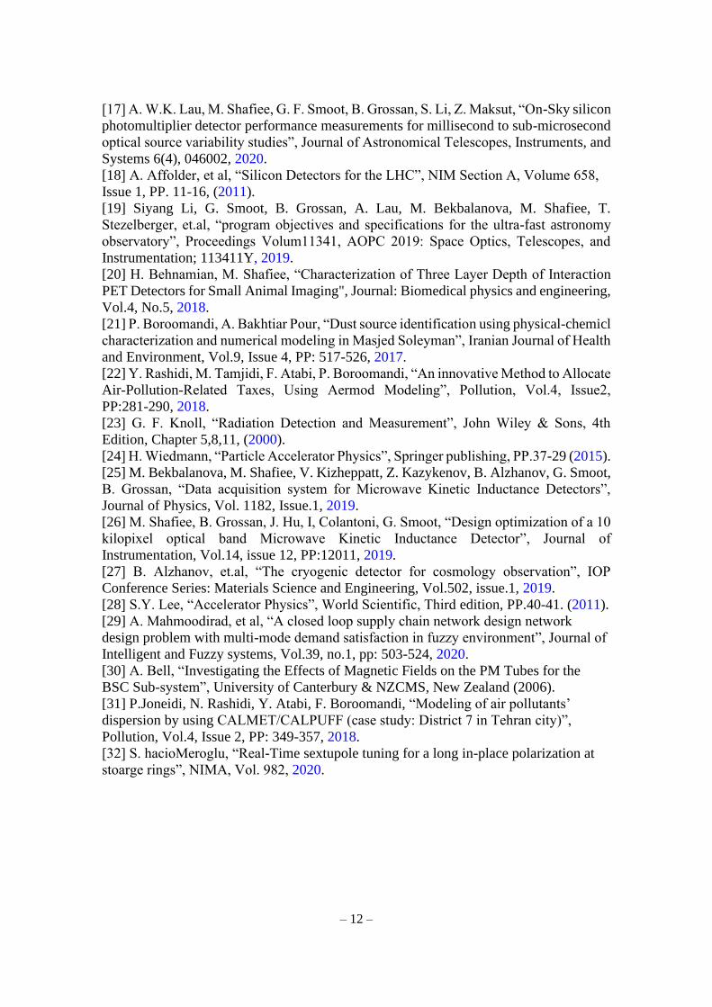
Figure 13. Deposited energy by photons in detectors.

As can be interfered from Fig. 10 to 13, most secondary particles reach the cell number 11 and

NaI has better results among others in terms of recording the number and deposited energies of

secondary electrons and photons. Since for using NaI we need photomultiplier tubes and they are

very sensitive to the magnetic fields, therefore, Si detectors can be a good candidate as BLM [32].

The semiconductor silicon detectors have the advantages of high resolution, linear response in a

wide range of energies, relatively fast response, high efficiency, ability to work in a vacuum

environment, insensitive to the magnetic field, and possibility to be constructed in various forms.

Then by placing the Si detector with the same size only in the place of cell 11 and running the

simulation again, we will achieve the recorded data as shown in Table V.

TABLE V. The number and deposited energy of secondary particles and photons in the Si detector.

Deposited energy

of neutrons

(MeV)

Number

of

neutrons

Deposited

energy of

photons (MeV)

Number

of photons

Deposited energy

of electrons

(MeV)

Number

of

electrons

0.0038 0.5786 3.8981 0.9086 0.1610 0.0543

5. Conclusion

In this paper, we have studied the beam loss due to the magnet misalignment, magnet vibration

and magnet current fluctuations that causes the beam to experience a different magnetic field than

the nominal value. We have studied the behavior of beam when it sees different magnetic fields

inside the magnets. Consequently, we have calculated the deflection angle with respect to the

reference beam axis due to the mismatch in the magnetic field of dipole, quadrupole, and

sextupole magnets [32]. The deflection angles are obtained to be between 0.5 to 6 degrees for

different magnetic fields of dipole magnet and 1.518 to 1.732 degrees for the sextupoles.

Therefore, we have considered that electron deflects with the angle of 3 degrees with respect to

the beam axis in all further calculations. We have shown that when a 3 GeV electron with 3

degrees of deflection angle hit the beam pipe, it will deposit all its energy there, and finally 34.8

secondary electrons with a total energy of 1073.3020 MeV, 139.7 photons with a total energy of

1467.999 MeV and 0.1 neutrons with a total energy of 1.32 MeV exit from the outer surface of

the beam pipe. We have then compared ionization chamber, NaI and Si detectors as candidates

for BLM, where it is concluded that NaI has better characteristics for this purpose [3]. However,

due to the sensitivity of photomultiplier tubes to the magnetic field, Si detector can be chosen as

– 11 –

a second-best candidate in accelerators. Also, it is shown that based on this deflection

angle, only some places around the beam pipe are appropriate to place the detector. We

have placed the Si detector in 10 cm distance from the beam pipe and have considered

the 3 GeV electron to be deflected with the angle of 3 degrees and hit the beam pipe in a

simulation done by MCNP [7]. It is concluded that only 0.05 electrons, 0.9 photons and

0.57 neutrons with the total deposited energy of 0.16 MeV, 3.89 MeV and 0.003 MeV,

respectively, will reach the detector.

References

[1] K. Wittenburg, F. Ridoutt, “Experience with the Electron and Proton Beam Loss

Monitor (BLM) Systems at HERA”, Proceeding of the 5th European Accelarator

Conference, 1612 (1996).

[2] P. Forck, “Lecture Notes on Beam Instrumentation and Diagnostics”, CreateSpace

Independent Publishing Platform, (2015).

[3] K. Wittenburg, “Beam Loss Monitors”, CERN-European Organization for Nuclear

Research, Issue 5, P.249 (2009).

[4] E.Ebrahimi Basabi, et. al, “Beam Profile measurement of ES-200 using secondary

electron emission monitor”, Iranian Journal of Physics Research, Vol.15, Issue 2, PP:253-

258, 2019.

[5] F. Ghasemi, et.al, “Construction of disk-loaded buncher for S-band low energy TW

electron linac”, IPAC12, WEPPD063, New Orleans, USA, 2012.

[6] B. Dehning, “Beam Loss Monitors at LHC”, CERN Yellow Report CERN-2016-

002, pp.303-318, (2016).

[7] Monte Carlo Methods, Codes, & Applications Group, Los Alamos National

Laboratory, (2017).

[8] H. Ghasem, et al. “Beam Dynamic of a New Low Emittance Third Generation

Synchrotron Light Source Facility”, Physical Review Special Topics-Accelerators and

Beams, Vol 18, 030710. (2015).

[9] J. Rahighi, et.al. “ILSF, a third-generation light source laboratory in Iran”, IPAC2013,

Shanghai China, TUOAB202, Vol 13, 2013.

[10] J. Rahighi, et al. “Recent Progress on the Development of Iranian Light Source

Facility (ILSF) Project”, IPAC16, Busan, Korea, PP: 2861-2863, 2016.

[11] J. Rahighi, et al., “Progress Status of the Iranian Light Source Facility”, IPAC14,

Dresden, Germany, 2014.

[12] M. Shafiee, S.A.H. Feghhi, J. Rahighi, “Numerical analysis of the beam position

monitor pickup for the Iranian light Source Facility”, NIMA, Vol. 847, PP: 162-170,

2017.

[13] M. Shafiee, SAH. Feghhi, J. Rahighi, “Experimental Performance Evaluation of

ILSF BPM Data Acquisition System”, Measurement, Vol.100, PP.205-212. 2017.

[14] A. Molaee, et.al “General Consideration for button BPM”, IPAC14, Dresden,

Germany, 2014.

[15] M. Shafiee, H. Behnamian, S.A.H. feghhi, “A Study of wake potentials for the

pickups in storage ring”, Journal of instrumentation, Vol.12, issue 12, 2017

[16] M. Shafiee, SAH Feghhi, J. Rahighi, “Analysis of de-noising methods to improve

the precision of the ILSF BPM electronic readout system”, Journal of Instrumentation,

Vol.11, 2016.

– 12 –

[17] A. W.K. Lau, M. Shafiee, G. F. Smoot, B. Grossan, S. Li, Z. Maksut, “On-Sky silicon

photomultiplier detector performance measurements for millisecond to sub-microsecond

optical source variability studies”, Journal of Astronomical Telescopes, Instruments, and

Systems 6(4), 046002, 2020.

[18] A. Affolder, et al, “Silicon Detectors for the LHC”, NIM Section A, Volume 658,

Issue 1, PP. 11-16, (2011).

[19] Siyang Li, G. Smoot, B. Grossan, A. Lau, M. Bekbalanova, M. Shafiee, T.

Stezelberger, et.al, “program objectives and specifications for the ultra-fast astronomy

observatory”, Proceedings Volum11341, AOPC 2019: Space Optics, Telescopes, and

Instrumentation; 113411Y, 2019.

[20] H. Behnamian, M. Shafiee, “Characterization of Three Layer Depth of Interaction

PET Detectors for Small Animal Imaging", Journal: Biomedical physics and engineering,

Vol.4, No.5, 2018.

[21] P. Boroomandi, A. Bakhtiar Pour, “Dust source identification using physical-chemicl

characterization and numerical modeling in Masjed Soleyman”, Iranian Journal of Health

and Environment, Vol.9, Issue 4, PP: 517-526, 2017.

[22] Y. Rashidi, M. Tamjidi, F. Atabi, P. Boroomandi, “An innovative Method to Allocate

Air-Pollution-Related Taxes, Using Aermod Modeling”, Pollution, Vol.4, Issue2,

PP:281-290, 2018.

[23] G. F. Knoll, “Radiation Detection and Measurement”, John Wiley & Sons, 4th

Edition, Chapter 5,8,11, (2000).

[24] H. Wiedmann, “Particle Accelerator Physics”, Springer publishing, PP.37-29 (2015).

[25] M. Bekbalanova, M. Shafiee, V. Kizheppatt, Z. Kazykenov, B. Alzhanov, G. Smoot,

B. Grossan, “Data acquisition system for Microwave Kinetic Inductance Detectors”,

Journal of Physics, Vol. 1182, Issue.1, 2019.

[26] M. Shafiee, B. Grossan, J. Hu, I, Colantoni, G. Smoot, “Design optimization of a 10

kilopixel optical band Microwave Kinetic Inductance Detector”, Journal of

Instrumentation, Vol.14, issue 12, PP:12011, 2019.

[27] B. Alzhanov, et.al, “The cryogenic detector for cosmology observation”, IOP

Conference Series: Materials Science and Engineering, Vol.502, issue.1, 2019.

[28] S.Y. Lee, “Accelerator Physics”, World Scientific, Third edition, PP.40-41. (2011).

[29] A. Mahmoodirad, et al, “A closed loop supply chain network design network

design problem with multi-mode demand satisfaction in fuzzy environment”, Journal of

Intelligent and Fuzzy systems, Vol.39, no.1, pp: 503-524, 2020.

[30] A. Bell, “Investigating the Effects of Magnetic Fields on the PM Tubes for the

BSC Sub-system”, University of Canterbury & NZCMS, New Zealand (2006).

[31] P.Joneidi, N. Rashidi, Y. Atabi, F. Boroomandi, “Modeling of air pollutants’

dispersion by using CALMET/CALPUFF (case study: District 7 in Tehran city)”,

Pollution, Vol.4, Issue 2, PP: 349-357, 2018.

[32] S. hacioMeroglu, “Real-Time sextupole tuning for a long in-place polarization at

stoarge rings”, NIMA, Vol. 982, 2020.