PAPER www.rsc.org/softmatter | Soft Matter

Study of blood flow impact on growth of thrombi using a multiscale model

Zhiliang Xu,*a Nan Chen,a Shawn C. Shadden,b Jerrold E. Marsden,c Malgorzata M. Kamocka,d

Elliot D. Rosend and Mark Alber*a

Received 21st July 2008, Accepted 3rd October 2008

First published as an Advance Article on the web 12th December 2008

DOI: 10.1039/b812429a

An extended multiscale model is introduced for studying the formation of platelet thrombi in blood

vessels. The model describes the interplay between viscous, incompressible blood plasma, activated and

non-activated platelets, as well as other blood cells, activating chemicals, fibrinogen and vessel walls.

The macroscale dynamics of the blood flow is represented by the continuous submodel in the form of

the Navier–Stokes equations. The microscale cell-cell interactions are described by the stochastic

Cellular Potts Model (CPM). Simulations indicate that increase in flow rates leads to greater structural

heterogeneity of the clot. As heterogeneous structural domains within the clot affect thrombus stability,

understanding the factors influencing thrombus structure is of significant biomedical importance.

1 Introduction

The hemostatic system has evolved to prevent the loss of blood at

the site of vascular injury. The response is rapid to limit bleeding

and is regulated to prevent excessive clotting that can limit flow.

The processes that are involved in the assembly of a thrombus

(blood clot) include complex interactions among multiple

molecular and cellular components in the blood and vessel wall

occurring under fluid flow.

Formation of a thrombus (thrombogenesis) involves the close

interplay between many processes that occur at different scales

(subcellular, cellular and multicellular, et al.). In the past, these

processes have been studied separately.

The flowing bloodstream over the thrombus affects its growth

and development. Blood carries cellular and molecular compo-

nents to the thrombus for their incorporation into the structure.

These not only include coagulant and anticoagulant proteins but

platelets and blood cells. While histologic analysis of thrombi

formed in vivo reveals the incorporation of leukocytes and

erythrocytes, most models of thrombogenesis fail to include these

cells, viewing them as passive elements entrapped in the clot. On

the other hand, recent evidence suggests that cellular derived

micro-particles in blood are also required for thrombus

formation.

Furthermore, shear forces generated by the flowing blood can

dislodge elements from the structure. Moreover, the growing

thrombus may generate turbulence in the flow field with signifi-

cant consequences to growth properties. Vortices forming behind

the thrombus can trap platelets and blood cells and move them

back towards the clot. This entraps blood cells producing

a thrombus with heterogeneous domains that may affect clot

aDepartment of Mathematics, University of Notre Dame, Notre Dame, IN,46556, USA. E-mail: malber@nd.edu; zxu2@nd.edubCardiovascular Biomechanics Research Laboratory, Stanford University,Palo Alto, CA, 94305, USAcDepartment of Control and Dynamical Systems, CaltechPasadena, CA,91125, USAdDepartment of Medical and Molecular Genetics, Indiana UniversitySchool of Medicine, Indianapolis, IN, 46202, USA

This journal is ª The Royal Society of Chemistry 2009

stability. Hemodynamic parameters also affect processes at the

cellular and subcellular scale. Endothelial cells respond to

changes in flow. Not only does flow affect cell shape, but it also

influences gene expression patterns. The pattern of gene expres-

sion in endothelial cells cultured under flowing media in vitro is

more typical of resting cells, while inflammatory markers are

expressed by cells growing under static conditions.

Whereas most existing models describe continuous dynamics

at the macroscale related to platelet aggregation and coagu-

lation reactions, there is a reason to believe that many aspects

of the cascade are better modeled as discrete events at the

microscale. First, certain enzymes exhibit threshold effects on

the activation or inhibition of substrate proteins. Second,

some of the more complex aspects of the coagulation process

are poorly understood, and certainly there is no closed-form

set of differential equations for the system as a whole.

Moreover, more coarse-grained information is available at the

microscale, e.g., whether a certain protein factor must be

present at some minimal concentration for a reaction to take

place, and it can be incorporated into the model in the form

of discrete states.

Cell-based discrete models are used in a variety of problems

dealing with biological complexity. One motivation for this

approach is the enormous range of length scales of typical bio-

logical phenomena. The recent book3 reviews many of the cell-

based models. Treating cells as simplified interacting agents, one

can simulate the interactions of tens of thousands to millions of

cells and still have within reach the smaller-scale structures of

tissues and organs that would be ignored in continuum (e.g.,

partial differential equation) approaches. At the same time,

discrete stochastic models including the Cellular Potts Model

(CPM) can be made sophisticated enough to reproduce almost

all commonly observed types of cell behavior.11–13,19,36–37 The

CPM, which is an extension of the Potts model from statistical

physics, can be made sophisticated enough to reproduce almost

all commonly observed types of cell behavior. It has become

a common technique for simulating complex biological problems

including embryonic vertebrate limb development,12,23 tumor

growth17 and vasculogenesis.22

Soft Matter, 2009, 5, 769–779 | 769

We believe that various aspects of the development of thrombi

are best studied using a multiscale hybrid model combining

discrete and continuous submodels at different scales. In ref. 38

the authors introduced a basic multiscale two-dimensional model

of thrombus formation. The model combines submodels of all

interrelated factors that contribute to the formation of a blood

thrombus at three spatial scales: 1) the vessel wall scale, assuming

the diameter of the artery to be of the order of 100 microns, 2) the

cellular scale determined by the diameter of a platelet being of the

order of 1 micron, and 3) the inter-cellular scale of the fibrin fibril

network.

The stochastic CPM is used in this model to represent several

types of cells of different sizes and with different adhesivity

properties as well as to describe platelet-injury adhesion, platelet

activation, platelet-platelet binding, cell movement, cell state

changes and platelet aggregation. The incompressible Navier–

Stokes (NS) equations describe dynamics of viscous blood

plasma and the interface submodel couples the CPM with the

continuous model to describe the thrombus-blood plasma

interface. The CPM and the blood flow model respectively are

defined on the lattice and the volume that fills the finite difference

grid. The two computational grids are spatially superimposed.

In this paper, we further develop this multiscale model by

introducing additional types of blood cells and use it to study clot

formation under various flow conditions. In particular, we

describe the impact of flow shear stresses on the final positions in

the thrombi of the cells with different adhesive properties.

Furthermore, we employ the Lagrangian Coherent Structure

(LCS) method (these methods have a long history, with some

related techniques going back to ref. 26. We follow the method of

Haller;16 see the history of this subject in ref. 33 and in ref. 20) to

analyze the detailed flow structure near the clot to reveal the role

of blood flow in clot formation.

The paper is organized as follows. Section 2 provides biolog-

ical background on thrombus development. Section 3 presents

a brief overview of the extension of the multiscale computational

model. Section 4 contains an extended discussion of simulations

and model parameter selection, demonstrates the robustness of

the model and describes blood flow effects on the growth of

thrombus. Section 5 contains the conclusions.

2 Biological and modeling background

Following vascular injury, blood is exposed to prothrombotic

environments that promote rapid thrombus formation.

Thrombus formation is the result of two interrelated processes,

namely, platelet interactions and activation of the coagulation

pathway. Immediately after vessel damage, platelets adhere to

the site of vessel injury forming a single cell layer. Platelet

adhesion is promoted by the binding of platelet receptors GpIb/

V/IX to vonWillebrand factor (vWF) and GpIa/IIa and GpVI to

collagen in the subendothelial matrix of the vessel wall. However,

more limited endothelial damage which doesn’t denude the

endothelium and expose the subendothelial matrix also promotes

platelet binding. Conceivably, activated endothelial cells expose

long vWF multimeric chains released from endothelial Weibel-

Palade bodies.

Following adhesion, platelets form multicellular aggregates

mediated by the binding of the platelet GpIIb/IIIa receptor to

770 | Soft Matter, 2009, 5, 769–779

fibrin(ogen). In addition, platelets undergo activation involving

significant morphological changes, the exposure of new proteins

on the platelet surface and the extracellular release of contents of

alpha and dense granules found in resting platelets. These

contents include a variety of hemostatic proteins and molecules

that stimulate a variety of cells at the site of vessel injury.

Activated platelets also provide a phospholipid surface that

promotes the surface dependent coagulation reactions at the site

of injury.

In addition to platelet interactions, coagulation factor VII(a)

in the blood is exposed to its cellular receptor, TF, expressed on

cells in the vessel wall. Coagulation is initiated when FVIIa

binds to TF. The TF/FVIIa complex catalyzes conversion of FX

to FXa and FIX to FIXa, and initiates a complex network of

reactions that lead to rapid generation of thrombin, which

serves to convert fibrinogen to fibrin, the major matrix protein

in a thrombus, and activates FXIII to cross-link fibrin. In

addition, thrombin triggers a positive feedback loop of propa-

gation reactions. Thrombin is also a potent activator of resting

platelets and thus mediates recruitment of resting platelets

owing nearby in the blood. The activated platelets provide

a procoagulant surface that promotes coagulation enzyme

activity. Making matters more complex, thrombin also activates

the Protein C anticoagulant pathway that inhibits the loop of

propagation reactions by inactivating coagulation factors FVa

and FVIIIa.

In the past, subprocesses involved in thrombogenesis have

been studied as distinct disciplines. For example, the extrinsic

and intrinsic coagulation pathways have been modeled using the

feedback loops described in ref. 18 and 4. The multifaceted

models have been developed based on a large number of reac-

tion-diffusion equations with parameters related to many aspects

of clot growth such as flow rates, membrane binding site density

and concentration of calcium (see ref. 40,39,25). Several models

concentrated on specific aspects of the coagulation. In ref. 6 and

7 it was shown that activation threshold for an enzyme cascade

was affected by the flow rate, the size of the injury and initial

concentrations of active enzymes. The regulation of activation

threshold by levels of Factor-VII and XII and clotting time

sensitivity to zymogen concentrations has been studied using

spatially homogeneous and inhomogeneous systems. Ref. 5 and

40 studied clot growth and dissolution using spatially inhomo-

geneous systems.

There are a few constitutive models of clot formation as well.

A 1D linear viscoelastic clot model has been proposed,21 a 3-D

Maxwell model was developed for the study of coagulation of

whole blood,28 and a Newtonian fluid model in the form of

coupled convection-reaction-diffusion equations without platelet

deposits has been used.14,35 These models neglected the effect of

the growing clot on the flow field. A recent model2 incorporated

both rheological properties of the clot and multiple biochemical

reactions. They modeled clot formation and dissolution as the

growth/diminishment of a singular front (viscoelastic liquid clot)

in a sheer-thinning viscoelastic whole blood region. The

convection-reaction-diffusion equations have been used for

modeling platelet activation, extrinsic coagulation pathway and

fibrinolysis. Due to the extremely complicated nature of blood

clotting, these attempts usually focused on small subsets of the

entire process.

This journal is ª The Royal Society of Chemistry 2009

3 Multiscale computational model

Due to the multiscale nature of platelet aggregation and coagu-

lation reactions, capturing both the discrete events and the

continuous mechanics, of thrombus development is best modeled

as a hybrid composition of the two. The multiscale approach

takes advantage of relative simplicity and efficiency of the

macroscopic models, as well as the accuracy of the microscopic

models, and it is particularly helpful for studying the macro-

micro relationships of blood flow and platelet aggregation and

coagulation. It allows one to model in detail formation of the

thrombus as well as a boundary layer between thrombus and

blood flow, resulting in a description of different phases in

thrombus development and of mechanisms determining its shape

and internal structure.

3.1 Submodels at different scales

Our model consists of a set of submodels for processes involving

components at scales described in the previous section:

� Biochemical reaction submodel: we use a set of PDEs to

describe the net effect of biochemical reactions.

� Cell submodel: The discrete stochastic CPM represents

different types of cells as well as accounts for platelet-injury

adhesion, platelet activation, platelet-platelet binding, cell

movements, cell state changes and platelet aggregation.

� Flow submodel: The incompressible Navier–Stokes equa-

tions describe dynamics of viscous blood plasma.

� Interface submodel: The submodel couples the CPMwith the

continuous model to describe the thrombus-blood plasma

interface. The CPM and the blood flow model are defined on the

lattice and volume filling finite difference grid respectively. Two

computational grids are spatially superimposed.

The simulation of the thrombus development starts with

utilizing macroscale submodules involving optimized Navier–

Stokes and advection diffusion solvers. Subsequently, obtained

blood flow velocity field and thrombin distribution is fed into the

CPM describing individual cell behavior. On the other hand, cell

differentiation and cell state transition is determined based on

the chemical concentration derived from a sub-cellular module

based on the kinetic equations modeling coagulation pathway.

This information is used when simulating generation of fibril

which eventually form fibrin network. We assume that geometry

of the thrombus (boundary conditions) does not change

considerably during calculation of the flow velocity field. The NS

equations and advection-diffusion equations for the flow and

chemical distributions are solved with this boundary condition

provided by the CPM. The result in turn is used in the subsequent

CPM update. It is also assumed that during the CPM step flow

conditions (velocity and pressure) remain unchanged. The

updated CPM data (interface geometry and chemical concen-

trations) provide new boundary and initial conditions for the NS

advection-diffusion equations modules. The spatial coupling

between cellular and thrombus scales is achieved through mesh

refinement between the CPM cell lattice and the finite difference

grid. The chemical concentration, obtained from the sub-cellular

kinetic equations, is averaged to these grids to reduce the

computational complexity.

This journal is ª The Royal Society of Chemistry 2009

3.2 Stochastic cellular Potts model

The CPM is a cell-level, energy-minimization-based lattice

model, which uses an effective energy E coupled to external

fields, e.g., the local flow rate, to describe cell motion, cell-cell

interactions, cell adhesion, differentiation, division and hapop-

tosis. Each cell consists of many pixels (lattice sites). The distri-

bution of multidimensional indices associated with lattice sites

determines current system configuration. The effective energy of

the system mixes true energies, like cell-cell adhesion, and terms

that mimic energies, e.g., the response of a cell to a blood flow

and the constraint

E ¼ Eadhesion + Eflow + Edim (3.1)

Given an effective energy one can calculate the resulting cell

motion using Metropolis dynamics algorithm based on the

Monte-Carlo Boltzmann acceptance rule.24 More details of the

energy form used in the clot formation modeling can be found

from our previous publication.38

Our model involves eight types of cells (see Fig. 1). ‘‘Injury’’

and ‘‘Vessel’’ cells do not represent cells in the CPM and are used

only to indicate boundary of the vessel domain and place of

injury. During simulation, their positions and adhesion proper-

ties are fixed and platelets can adhere to their surfaces. New

platelets (inactivated) and blood cells are injected from the inlet

(left) side at a specified rate. When cells reach the outlet (right)

side of the simulation domain, they are removed from the system.

We impose the ‘‘no-flux’’ boundary condition on both upper and

lower boundaries so that cells would not move outside of the

domain.

When an inactivated platelet reaches the cite of the injury or

the ADP concentration of a platelet becomes higher than the set

threshold value, it changes its type to ‘‘activated’’ and starts

releasing thrombin which causes fibril generation. Generated

fibrils gradually form fibril network which increases thrombus

stiffness and prevents platelets from detaching from the

thrombus surface. The fibril level in the thrombus and activated

platelet cluster increases with the increase in thrombin concen-

tration. Thus, clusters consisting of activated platelets, have

different fibril levels and stiffness properties at initial and later

stages. In our CPM, we implement two different activated

platelet states (activated platelet and activated platelet with high

fibril level), with different flow responses.38

Platelet adhesion is mediated by plasma proteins bridging

receptors on adjacent platelets (gpIIbIIIa fibrinogen, vironect-

ing, von Willebrand Factor, gpV1-collagen, etc). It is difficult to

describe all details of cell-cell adhesion in the model. In the CPM

the cell-cell adhesion is described as an energy penalty function

term: low cell-cell adhesion energy represents strong adhesivity

between cells while high cell-cell adhesion energy represents weak

cell-cell adhesivity.

In the CPM, the adhesion energy is calculated by

Eadhesion ¼X

ði;j;kÞ;ði';j';k'ÞneighborsJsðsÞs 'ðs 'Þð1� dðsði; j; kÞ; s'ði'; j'; k'ÞÞÞ;

(3.2)

where d(s,s0) ¼ 0 if s s s0, and d(s,s0) ¼ 1 if s ¼ s0. These

conditions ensure that only the surface sites between different

Soft Matter, 2009, 5, 769–779 | 771

cells contribute to the adhesion energy. Each term under

summation sign is a product of the binding energy per unit

length, Jt(s)t0(s0), and the length of a contact between two

neighboring cells. Adhesive interactions act up to second-near-

est-neighbors. Ref. 15, 27 and 29 show that the adhesivity

between platelets and thrombus is strongly affected by the flow

shear rate on the thrombus surface. At low shear rate, the value

of adhesivity is low and it becomes higher with the increase of the

shear rate, eventually to a constant value. To describe the

dependence of the adhesivity on the shear rate, Jt(s)t0(s0) is

described as a function of the flow shear rate _g on the thrombus

surface:

JsðsÞs 'ðs 'Þ�_g�¼

8<:

Jh þ Je_gh � _g

_gh � _gl

; _g � _gt1

Jh _g � _gt1

(3.3)

where _gh and _gl are the high and low thresholds values of the

shear rate, and Jh and Je are adhesion energy constants.

3.3 Continuous submodels of blood flow and biochemical

reactions

Blood is a complex mixture of cells, proteins, lipoproteins and

ions by which nutrients and wastes are transported. Red blood

cells comprise approximately 40% of blood by volume. In

contrast to water, blood does not exhibit a constant viscosity at

all flow rates and is non-Newtonian in the microcirculatory

system (in small branches and capillaries). The normal blood

flow is laminar with secondary flows generated at curves or

branches. The Reynolds number varies from 1 in small arterioles

to approximately 4000 in the largest artery. Moreover, the blood

flow and pressure are unsteady, since the heart creates pulsating

conditions in all arteries. Depending on the artery and the flow

being modeled, the following main features are usually addressed

in a comprehensive blood modeling effort: vessel wall elasticity,

non-Newtonian viscosity, Fahraeus–Lindquist effect, motion of

particles in the fluid, Fahraeus effect, body forces, and temper-

ature. The Fahraeus–Lindquist effect accounts for the blood

viscosity dependence on the diameter of the vessel it travels

through. The Fahraeus effect is present when blood flows from

a large reservoir into a small circular cylindrical tube. As a result

the hematocrit in the tube is smaller than that in the reservoir.

Since we model the development of thrombus inside a blood

vessel of length approximately 10 times larger than the its

diameter, in our model, we simplify the vessel to be a straight

pipe. The vessel wall is assumed to be a rigid wall. Blood plasma

is treated as an incompressible fluid, which is modeled by the

two-dimensional incompressible Navier–Stokes equations that

take the form

Table 1 Coefficients of chemical components and source terms of equations

Species Di/cm2 s�1

ADP 2.56 � 10�6

TxA2 2.14 � 10�6

Prothrombin [PT] 3.32 � 10�7

Thrombin [T] 4.16 � 10�7

ATIII 3.49 � 10�7

772 | Soft Matter, 2009, 5, 769–779

vvu

vtþ ð

vu ,VÞ

vuþ 1

rVp ¼ m

rV2

vuþ

vf (3.4)

V ,vu ¼ 0 (3.5)

wherevu ¼ ðu; vÞ is the flow velocity, r is the density of the

blood plasma, p is the pressure, and m is the viscosity. We

impose the Dirichlet boundary condition (u,v) ¼ (0,0) on

no-slip boundaries.

The major goal of the paper is to study how blood flow affects

developing clots. For this reason, we apply a simple phenome-

nological model to describe the biochemical processes in the form

of the following system of reaction advection-diffusion equa-

tions35

vCk

vtþ V,ðCk

vu Þ ¼ DkV

2Ck þ Sk; k ¼ 1; 2; :::; 5 (3.6)

where Dk is a diffusion coefficient of the k-th chemical compo-

nent. Sk is the reaction source term of the k-th chemical

component due to the enzymatic reactions. This model is

comprised of equations describing platelet released agonist,

adenosine diphosphate (ADP), and synthesized agonist, throm-

boxane (TxA2), which can be inhibited via 1st order reactions;

prothrombin; thrombin; and antithrombin III (ATIII), which

inhibits thrombin.

Table 1 lists coefficients of chemical components used in the

equations, the source terms and initial concentrations in blood.

Here symbol Ck represents chemical concentration, [AP] and

[RP] are concentrations of the activated and resting platelets,

which are computed from the discrete CPM. (See ref. 35 for the

parameter values appearing in the source term.)

The activation condition for the platelets depends on the

concentrations of the chemical components as well as blood flow

conditions. Platelet activation is partially triggered by the

exposure to shear stresses which are higher than certain threshold

values.10 In the problems studied in the paper, stresses are lower

than the threshold values.

We assume that activation of platelets occurs when the

concentration of chemical components is higher than a specified

threshold. The valid activator concentration is calculated

according to:35

U ¼ ½ADP�½ADPcrit�

þ ½TxA2�½TxA2crit�

þ ½Thrombin�½Thrombincrit�

(3.7)

where acrit is the threshold concentration of that agonist for

platelet activation, which is obtained from ref. 35. Once the valid

activator concentration U around a platelet is higher than the

threshold value Ta, the platelet is activated.

Si Init. Conc.

likpa[RP] � k1,j[ADP] 0.0 mMspj[AP] � k1,j[TxA2] 0.0 mM�b[PT](fat[AP] + frt[RP]) 1.0 mM�G[T] + [PT](fat[AP] + frt[RP]) 0.0 U�Gb[T] 2.844 mM

This journal is ª The Royal Society of Chemistry 2009

3.3.1 Parabolic and pulsatile flow models. There is evidence

that vascular fluid dynamics plays an important role in the

development of the thrombus. To mimic physiological flow

conditions, we used a sinusoidal time-dependant velocity func-

tion to model the effect of pulsatility. We impose on the inlet

section that

u ¼ u0(1.0 + 3 sin(wt)) (3.8)

where u0 is mean velocity and 3 is an amplitude of the pulsatility

relative to the mean velocity. The period of oscillation is w ¼ 1 s.

We also assume that the upstream flow is laminar and has

a parabolic profile, resulting in the following inlet velocity

uðhÞ ¼ u

�1:0þ 1:44

ffiffiffif

pþ 2:15

ffiffiffif

plog10

�1� 2h

D

��; (3.9)

v ¼ 0.0 (3.10)

where u(y) is a x-velocity component at a distance h from the

center of the pipe on the inlet, v is a y-velocity component, D is

diameter of the pipe and f is the friction factor, which is set to be f

¼ 0.01. In general, the friction factor depends on the Reynolds

Number of the pipe flow. Here we assume that the Reynolds

Number is moderate and the inner side of the blood vessel is

smooth in the upstream flow direction.

3.3.2 Non-Newtonian blood viscosity model. To identify the

role of the non-Newtonian property of the blood, we imple-

mented widely used Carreau-Yasuda model8 for the blood

viscosity

m�_g�¼ mN þ ðm0 � mNÞ

�1þ

�l _g

�aðn�1Þ=a(3.11)

where viscosity m is a function of the shear rate _g ¼ffiffiffiffiffiffiffiffiffiffiffiffiffiffiffiffiffi2D : D

qwith the following rate of deformation tensor

D ¼ 1

2

�Vvuþ ðV

vu ÞT

�: (3.12)

Here a, n and l are empirically determined parameters.

In this paper we use the following values a¼ 2, n¼ 0.3568, l¼3.313 s. Parameters mN and m0 are chosen as mN ¼ 0.0345 g cm�1

s�1 and m0 ¼ 0.56g cm�1 s�1 respectively. These parameter values

were taken from a study of the pulsatile flow of blood through

stenotic arteries.1 The calibration of these parameter values was

carried out by a simulation study to show the rheological

behavior of blood flow and to calculate the magnitude of the wall

shear stresses. In simulations with blood being treated as New-

tonian flow, the viscosity m value is set at m ¼ 0.04 g cm�1 s�1

based on the experimental data.

3.4 Coupling between continuous and discrete submodels

3.4.1 Thrombus-plasma interface. We use volume of fluid

approach to explicitly track the interface between developing the

thrombus (or platelet aggregates at an earlier stage) and blood

plasma. A thrombus, in principle, can be treated as a gel-like

matter, and exhibit viscoelastic behavior. In this paper, we make

the following assumptions to simplify the description of the

interactions:

This journal is ª The Royal Society of Chemistry 2009

� Blood plasma (the liquid phase) and the thrombus (visco-

elastic matter phase) are assumed to be separated by a sharp

interface called thrombus-plasma interface.

� It is also assumed that within a time step of the Navier–

Stokes PDE solver, the thrombus domain does not change.

Based on these assumptions, we solve Navier–Stokes equa-

tions to update the flow velocity and pressure fields inside

thrombus domain which is fixed during a time step of the PDE

cycle. The updated velocity and pressure fields, in turn, drive the

cells’ motion and aggregation, resulting in thrombus shape

change during the subsequent CPM time step.

All cells in the simulation domain are divided into two types:

cells floating in blood stream and cells on the thrombus. We use

two different methods to handle cell-fluid interactions for two

types of cells. Floating cells are not connected to each other and

it would be very computationally expensive to take all individual

cell geometries into account in solving the Navier–Stokes equa-

tion. The effects of the small floating cell on the blood velocity

distribution are very weak and are ignored in our model to save

calculation time. We do not take floating cells into account in the

boundary condition setup for Navier–Stokes equations. The

motion of floating cells is calculated from the blood velocity

distribution and the flow energy of floating cells depends on the

blood velocity. The cells that are located on the thrombus are

connected to each other by fibers and are treated as a stiff

obstacle in solving the Navier–Stokes equations. Since they are

treated as the stiff boundary, the blood velocities for thrombus

cells are zero and the motion of them cannot be determined from

the blood velocity. We use the blood pressure to determine the

thrombus cells’ motion, and the flow energy term of the

thrombus cells depends on blood pressure. The blood pressure

on the cells that are located on the thrombus boundary is non-

zero and drives them to move towards the interior of the

thrombus, compressing internal thrombus cells. However,

the volume constraint on the internal thrombus cells resists the

compression from the outside cells and the balance between two

trends is obtained from the energy-minimizing principle of the

CPM.

The evolution of the interface between thrombus and blood

plasma is driven by the platelet aggregation and coagulation and

its dynamics is described by the CPM. To track the interface, we

superimpose the CPM cell lattice (grid) on and align with the

PDE grid (see Fig. 2).

The thrombus-plasma interface is identified on the CPM

lattice as a union of outer boundaries of cells located in the

current surface of a thrombus. The interface is projected onto the

PDE grid to provide boundary conditions for the PDE solution

step. We employ no slip boundary conditions.

3.4.2 Impact of the blood flow on a moving cell. We use the

flow energy term in the CPMHamiltonian to describe the impact

of the blood flow on the cells. The flow energy terms for different

types of cells are calculated from the flow velocity distribution or

flow pressure.

Cells with high level of fibril concentration are very stiff and

aggregate together to form the thrombus. In this model, they are

treated as obstacles for the blood flow. The flow force applied to

one of these type cells is calculated as an integral of blood

pressure along a cell membrane:

Soft Matter, 2009, 5, 769–779 | 773

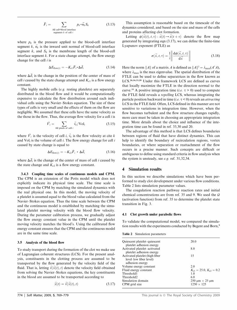
Table 2 Simulation parameters

Quiescent platelet–quiescentplatelet adhesion energy

20.0

Activated platelet–activatedplatelet adhesion energy

8.0

Activated platelet (high fiberlevel–low fiber level)adhesion energy

15

Volume energy constant 2.0Fluid energy constant Ke1 ¼ 25.0, Ke2 ¼ 0.2Threshold1 1.0Threshold2 6.0Simulation domain 250 mm � 25 mmCPM grid size 1250 � 125

vFi ¼

XAll cell-blood interface

segments k of cell i

pk,vnkSk (3.13)

where pk is the pressure applied to the blood-cell interface

segment k,vnk is the inward unit normal of blood-cell interface

segment k, and Sk is the membrane length of the blood-cell

interface segment k. For a state change attempt, the flow energy

change for the cell i is

DEflowðiÞ ¼ �Ke1

vFi,D

vdi (3.14)

where Dvdi is the change in the position of the center of mass of

cell i caused by the state change attempt and Ke1 is a flow energy

constant.

The highly mobile cells (e.g. resting platelets) are separately

distributed in the blood flow and it would be computationally

expensive to calculate the flow distribution around each indi-

vidual cells using the Navier–Stokes equation. The size of these

types of cells is very small and the effects of them on the flow are

negligible. We assumed that these cells have the same velocity as

the those in the flow. Thus, the average flow velocity for a cell i is

vVi ¼

XAll pixels of cell i

vvk=Voli (3.15)

wherevVi is the velocity of cell i,

vvk is the flow velocity at cite k

and Voli is the volume of cell i. The flow energy change for cell i

caused by state change is equal to

DEflowðiÞ ¼ �Ke2

vFi , D

vdi (3.16)

where Dvdi is the change of the center of mass of cell i caused by

the state change and Ke2 is a flow energy constant.

3.4.3 Coupling time scales of continuous models and CPM.

The CPM is an extension of the Potts model which does not

explicitly indicate its physical time scale. The time scale is

imposed on the CPM by matching the simulated dynamics with

the real physical one. In this model, the moving velocity of

a platelet is assumed equal to the blood value calculated from the

Navier–Stokes equation. Thus the time scale between the CPM

and the continuous model is established by matching the simu-

lated platelet moving velocity with the blood flow velocity.

During the parameter calibration process, we gradually adjust

the flow energy constant value in the CPM until the platelet

moving velocity matches the blood’s. Using the calibrated flow

energy constant ensures that the CPM and the continuous model

are in the same time scale.

3.5 Analysis of the blood flow

To study transport during the formation of the clot we make use

of Lagrangian coherent structures (LCS). For the present anal-

ysis, constituents in the clotting process are assumed to be

transported by the flow generated by the velocity field of the

fluid. That is, lettingvvð

vxðtÞ; tÞ denote the velocity field obtained

from solving the Navier–Stokes equations, the key constituents

in the blood are assumed to be transported according tovxðtÞ ¼

vvð

vxðtÞ; tÞ (3.17)

774 | Soft Matter, 2009, 5, 769–779

This assumption is reasonable based on the timescale of the

dynamics considered, and based on the size and mass of the cells

and proteins affecting clot formation.

Letting fðvxðtÞ; t; sÞ :

vxðtÞ/

vxðtþ sÞ denote the flow map

generated by integrating eqn (3.17), we can define the finite-time

Lyapunov exponent (FTLE) as

sðvx; t; sÞ ¼ 1

s

dfð

vx; t; sÞdvx

(3.18)

Here the norm kAk of a matrix A is defined as kAk2 ¼ lmax(A*A),

where lmax is the max eigenvalue. The spatial distribution of the

FTLE can be used to define separatrices in the flow known as

LCS.26,16,33,20 Under this framework LCS are defined as curves

that locally maximize the FTLE in the direction normal to the

curve.33 A positive integration time (i.e. t > 0) used to compute

the FTLE field reveals a repelling LCS, whereas integrating the

particle position backward in time (i.e. t< 0) reveals an attracting

LCS in the FTLE field. Often, LCS defined in this manner are not

sensitive to variations in integration time. However, when the

flow becomes turbulent and the flow structure changes rapidly,

more care must be taken in choosing an appropriate integration

time. More details about the choice and influence of the inte-

gration time can be found in ref. 33,30 and 20.

The advantage of this method is that LCS defines boundaries

between regions of fluid that have distinct dynamics. This can

help to identify the boundary of recirculation regions, vortex

boundaries, or where separation or reattachment of the flow

occurs in a precise manner. Such concepts are difficult or

ambiguous to define using standard criteria in flow analysis when

the system is unsteady, see e.g. ref. 31,32,34.

4 Simulation results

In this section we describe simulations which have been per-

formed to study clot development under various flow conditions.

Table 2 lists simulation parameter values.

The coagulation reaction pathway reaction rates and initial

chemical concentrations are from ref. 35 and 9. We used the U

(activation function) from ref. 35 to determine the platelet state

transition in Fig. 3.

4.1 Clot growth under parabolic flows

To validate the computational model, we compared the simula-

tion results with the experiments conducted by Begent and Born,9

This journal is ª The Royal Society of Chemistry 2009

Fig. 3 Cell state transition map.

Fig. 4 The effect of blood flow rate on clot growth. The clot size refers to

the number of platelets the thrombus is composed of at time 25 s.

Fig. 1 Different types of cells in the model of thrombus development.

Fig. 2 Diagram of the thrombus-plasma interface. a) The thrombus-

plasma interface in the simulation. b) Spatially coupled finite difference

grid and the CPM lattice.

in which they found that the size of the resulting thrombus first

increased and then decreased with increase of blood flow

velocity. We ran simulations with different mean blood flow

velocities ranging from 200 mm s�1 to 1200 mm s�1 to select free

parameters in our model and test whether our model was capable

of reproducing this result. We set 3 ¼ 0 to eliminate the pulsatile

flow effect from this bench mark simulation. In addition, we also

investigated clot development under blood flows with different

viscosity values (m ¼ 0.04, 0.02, 0.01, 0.005 Poise). We were able

This journal is ª The Royal Society of Chemistry 2009

to reproduce the trend of the clot growth and show that it was of

the same order of magnitude as in the experiment.

Fig. 4 shows distribution of sizes of simulated clots in numbers

of coagulated platelets obtained after 25 s, for different blood

flow velocities and viscosities. For normal blood viscosity of m ¼0.04 Poise, the simulation result is very similar to the experi-

mental result described in ref. 9 (Fig. 4b). Simulations demon-

strated that growth of the thrombus was strongly affected by two

competing factors: the rate at which platelets were supplied by

the blood flow to the thrombus, and intensity of shear force

which prevented platelets from adhering to the thrombus. When

the blood flow rate is low, platelets supply rate plays dominant

role. When blood flow rate is high, the shear force increases to

such an extent that it prevents platelets from adhering to the

thrombus.

Simulations also demonstrated that growth of thrombi was

not greatly influenced by the blood viscosity. In a reasonably

wide range of values of viscosity (0.01 # m # 0.04), growth of

thrombi showed similar characteristics.

4.2 Clot growth under Newtonian pulsatile flow

Fig. 5 displays clot size vs. various flow rates, viscosities and

pulse strengths. Notice that under the normal blood viscosity (m

¼ 0.04 Poise), clot development has similar characteristics. For

the pulse strength varying between 0.0 and 0.6, the maximum of

the clot size occurs at the flow rate between 400 mm s�1 and 600

mm s�1. On the other hand, for the extremely low viscosity (m ¼0.005 Poise), clot development has different characteristics.

When there is no pulse, clot size first increases with respect to the

increment of the flow rate, then at flow rate of 1000 mm s�1 it

reaches its maximum, and then starts to decrease. However, clot

size keeps increasing as the flow rate increases for the pulse

strength of 3 ¼ 0.2, 0.4 and 0.6 respectively.

For the fluid viscosity between 0.04 Poise and 0.005 Poise, the

pulsatile flow changes the dynamics of the clot development

quantitatively but not qualitatively. This means that for different

pulse strength, the maximum of the clot size occurs at different

flow rates. Nevertheless, for viscosity m¼ 0.02 and 0.01 Poise, the

size of the resulting thrombus still first increases and then

decreases with increase of blood flow velocity.

Soft Matter, 2009, 5, 769–779 | 775

Fig. 5 The effect of pulse parameters and viscosity on clot growth. The pulse strengths are: (a) 3 ¼ 0.2, (b) 3 ¼ 0.4, and (c) 3 ¼ 0.6 respectively. The clot

size is given in number of platelets in the thrombus after 25 s.

4.3 Clot growth under non-Newtonian pulsatile flow

Fig. 6 displays clot size vs. various flow rates for pulse strengths

(3 ¼ 0.0, 0.1 and 0.2). After comparing with Fig. 4 we observe

that, in the absence of a pulse, non-Newtonian flow effect is

negligible within the range of flow rates we study. Moreover,

when pulse strength is small (3¼ 0.1), the growth of the clot is not

affected by the pulsatile flow. However, increase in the strength

of the pulsatile flow changes clot size dramatically. When pulse

Fig. 6 The effect of non-Newtonian flow on clot growth. The pulse

strength is 3 ¼ 0.0, 0.1, 0.2 respectively. Clot size refers to the number of

platelets the clot is composed of after 25 s.

776 | Soft Matter, 2009, 5, 769–779

strength is 3 ¼ 0.2, clot size is significantly smaller. (See Fig. 6 for

a comparison.)

4.4 Distribution of cells in clots formed with different flow rates

Clots in Fig. 7 and Fig. 8 simulated for the flow rates from 0.1 cm

s�1 to 20.0 cm s�1 all have inhomogeneous internal structure. At

the same time, the positions of clusters of blood cells are very

different. Namely, most blood cells are located in the middle of

the clot in Fig. 7a, in the upper part of Fig. 7b and in the lower

part of Fig. 7d. This shows that formulation of the internal clot

structure is significantly influenced by the blood flow.

To simplify the analysis of the clots’ internal structure we

divide it into two equal parts (front and back) and compare

numbers of blood cells in those parts. For low blood flow rates

(0.1 cm s�1 and 1 cm s�1), the number of blood cells in the front

part is higher than in the back part (the ratio is higher than 1.0).

For high blood flow rates (>1.0 cm s�1) the ratio is close to 1.0,

implying that blood cells are homogeneously distributed in the

front and back parts. For a flow rate of 20.0 cm s�1, flow vorticity

is observed to bring some platelets to the back side of the clot.

However, the flow vorticity is weak and flow does not flush larger

blood cells to the back side of the clot.

The effect of the low rate on the complexity of the clot struc-

ture is observed in the development of thrombi generated

following vascular injury in experimental animals. Fig. 7f is

a frame from a video monitoring a single optical plane through

This journal is ª The Royal Society of Chemistry 2009

Fig. 7 The effect of flow rate on the blood cell distribution inside the clot. Flow rates v are (a) v ¼ 0.1 cm s�1.

Fig. 8 The effect of flow rate on the blood cell distribution inside the

clot. For each simulation in Fig. 7, we divide the clot into two equal front

and back parts. The flow is from the left (front part) to the right (back

part). The ratio r is defined by r ¼ Nfront/Nback, where Nfront and Nback

represent numbers of blood cells in the front and back parts of the clot,

respectively.

a clot developing in a mouse mesenteric vessel following a laser

induced injury. The frame shows a heterogeneous structure that

includes platelets (green) and fibrin (blue) as well as blood cells

(black ‘‘holes’’ excluding dextran (red) in blood). The role of

perturbations in the flow field leading to the entrapment and

incorporation of blood cells and the irregular thrombus structure

is more evident in the video recording than in a single frame. The

ability of the simulation to predict the effect of flow on clot

structural features is the subject of future studies.

4.5 Analysis of the blood flow near the clot

Here we apply the methodology described in Section 3.5 to

understand the role of the blood flow near the clot. Fig. 9 plots

the forward-time FTLE field at 6 instances during the clot

formation stage. There is a well-defined repelling LCS that exists

throughout the clotting process, which is defined by the curve of

high FTLE (shown in red). Proximal to the clot, the LCS remains

close to the vessel wall. Nearing the clot, the LCS extends toward

This journal is ª The Royal Society of Chemistry 2009

the center of the vessel and encloses a region that contains both

portions of the blood clot. This LCS appears to terminate on the

distal portion of the clot, away from the vessel wall. Distal to the

second portion of the clot, there exists a separate LCS, which

terminates on the vessel. The integration time used to compute

the FTLE fields was t ¼ 0.3 s.

In the case where the peak free-stream flow speed is 0.1 cm s�1,

there is no recirculation present behind the clot throughout the

clotting process. The Reynolds number for this flow is Re ¼0.001, based on the vessel diameter and average flow speed.

Therefore, the flow is highly viscous and is able to remain

attached downstream from the clot.

For the case where the peak free-stream flow speed is 5 cm s�1,

two clots that are initially separate, but close, form and quickly

combine to form a single clot. As these clots develop, an interior

region of recirculation exists between them. This region is bound

by the repelling LCS shown in Fig. 9 that propagates proximal to

the clot region close to the vessel wall and covers the majority of

the region where the clot develops. Therefore no transport occurs

between this interior recirculation region and the surrounding

blood flow, except entrainment of flow near the vessel wall. This

thin layer of blood bound by the LCS proximal to the clotting

region also constitutes fluid that eventually grows the clot. Distal

to the clot, there is a small region of recirculation. This small

recirculation region is partially bound by a separate repelling

LCS that terminates on the vessel wall downstream from the clot.

This LCS is separate from the primary LCS bounding much of

the clotting region. The gap between this LCS and the distal side

of the clot permits entrainment and detrainment between this

small region of recirculation behind the clot and the ambient

flow. However, the rate of entrainment and detrainment is small

during the clotting process and does not appear to affect the clot

formation significantly.

5 Conclusions

Since the hemostatic system has evolved to stem the loss of blood

following damage to blood vessels, understanding the parame-

ters affecting clot structural integrity has important biomedical

Soft Matter, 2009, 5, 769–779 | 777

Fig. 9 Forward-time FTLE field at 6 instances during clot formation. A well-defined LCS is present that defines the boundary between the region of

blood propagating downstream and blood that recirculates and clots. The integration time used to produce these plots was t ¼ 0.3 s.

implications. Furthermore, intravascular clots formed in

response to damage that does not cause vessel rupture presents

potentially serious pathological conditions. These intravascular

clots (thrombi) can grow and restrict blood flow, causing

pathology in the tissues supplied by the vessel. Additionally,

unstable thrombi can shed emboli (clot fragments) that can

embed in vessels of the lungs or brain potentially causing

pulmonary embolisms or ischemic strokes, respectively. These

conditions result in a significant number of deaths in the US, and

the rate is expected to increase as the population ages.

This paper describes the incorporation of additional hemo-

dynamic complexity into a computational model of thrombus

development first introduced in ref. 38. Simulations using this

updated model indicate that increasing flow rates lead to greater

structural heterogeneity. These irregular clots include domains

with distinct compositions and with different mechano-elastic

properties. Differential compression by adjacent domains in

response to changing forces on the thrombus can lead to frac-

tures at the interface between domains.

We used LCS to determine the region of blood that is trans-

ported to the clot. (We only considered the kinematic affect of

the blood flow on transport near the clot.) The computation of

LCS can also be applied to three-dimensional data,20 as has

already been done in other cardiovascular applications.34 Qual-

itatively, we expect future computations of LCS using three-

dimensional blood clot formation data will reveal similar regions

of recirculation and transport mechanisms. The typical Reynolds

numbers for flow around the clots considered here are sufficiently

low that we do not expect any transition to turbulence for three-

dimensional flow. However, the rough surface of the blood clot

often leads to complex secondary instabilities for the flow near

778 | Soft Matter, 2009, 5, 769–779

the clot. Moreover, previous experience in applying these

computation to three-dimensional blood flow data leads us to

expect that the three-dimensional simulations may reveal more

complex stirring of the blood in the vicinity of the clot due to the

increase degree of freedom of transport. This hypothesis will be

investigated further in our future work on three-dimensional

blood clot formation simulations.

We are currently working on a three dimensional extension of

the multiscale approach and incorporating into the model

platelet specific dynamics and the biochemical effects influencing

platelet transport near the clot boundary. To study these

dynamics, a much more highly resolved understanding of the

flow must be obtained near the clot boundary, which requires

a fully resolved three-dimensional calculation.

Acknowledgements

This work was partially supported by NSF Grant DMS-0800612

to MA, ZX and NC and by NIH grant HL073750 to EDR.

References

1 S. Amornsamankul, B. Wiwatanapataphee, Y. H. Wu andY. Lenbury, Intl. J. of Biomedical Sciences, 2006, 1(1), 42–46.

2 M. Anand, K. Rajagopal and K. R. Rajagopal, Pithily HaemostThromb, 2005, 34(2–3), 109–120.

3 A. Anderson, M. Chaplain and K. Rejniak, Single Cell-Based Modelsin Biology and Medicine, Birkhaser, 2007.

4 S. A. Baldwin and D. Basmadjian, Ann Biomed Eng, 1994, 22(4), 357–370.

5 I. A. Barynin, I. A. Starkov and M. A. Khanin, Izv Akad Nauk SerBiol, 1999, 1, 59–66.

6 E. Beltrami and J. Jesty, Proc Natl Acad Sci U S A, 1995, 92(19),8744–8748.

7 E. Beltrami and J. Jesty, Math Biosci, 2001, 172(1), 1–13.

This journal is ª The Royal Society of Chemistry 2009

8 R. B. Bird, R. C. Armstrong and O. Hassager, Dynamics of PolymerLiquids, 2nd edn, Wiley, New York, vol. 1, 1987.

9 N. Begent and G. V. Born, Nature, 1970, 227, 926–930.10 C. H. Brown, L. B. Leverett, C. W. Lewis, C. P. Alfrey and

J. D. Hellums, J Lab Clin Med, 1975, 86, 462–471.11 R. Chaturvedi, C. Huang, B. Kazmierczak, T. Schneider, J. Izaguirre,

T. Glimm, B. Hentschel, J. Glazier, S. Newman andM. S. Alber, J. R.Soc. Interface, 2005, 2(3), 237–253.

12 T. M. Cickovski, C. Huang, R. Chaturvedi, T. Glimm, H. Hentschel,M. S. Alber, J. A. Glazier, S. A. Newman and J. A. Izaguirre, IEEE/ACM Trans. Comput. Biol. Bioinformatics, 2005, 2(4), 273–288.

13 T.M.Cickovski,K.Aras,M. Swat,R.Merks,T.Glimm,H.Hentschel,M. S. Alber, J. A. Glazier, S. A. Newman and J. A. Izaguirre,Computing in Science and Engineering, 2007, 9(4), 50–60.

14 A. L. Fogelson, SIAM JAM, 1992, 52, 1089–1110.15 S. Goto, Y. Ikeda, E. Saldivar and Z. M. Ruggeri, Journal of Clinical

Investigation, 1998, 101(2), 479–486.16 G. Haller, Physica D, 2001, 149(4), 248–277.17 Y. Jiang, J. Pjesivac-Grbovic, C. Cantrell and J. P. Freyer, Biophys J,

2005, 89(6), 3884–3894.18 M.A.Khanin andV.V. Semenov, J. TheorBiol, 1989, 136(2), 127–134.19 M. A. Knewitz and J. C. M. Mombach, Comput Biol Med, 2006,

36(1), 59–69.20 F. Lekien, S. C. Shadden and J. E. Marsden, Journal of Mathematical

Physics, 2007, (6), 065404.21 E. S. Lobanova and F. I. Ataullakhanov, Phys. Rev. Lett., 2003, 91,

138301.22 R. Merks, S. V. Brodsky, M. S. Goligorksy, S. A. Newman and

J. A. Glazier, Dev Biol, 2006, 289(1), 44–54.23 S. Newman, S. Christley, T. Glimm, H. Hentschel, B. Kazmierczak,

Y. Zhang, J. Zhu and M. S. Alber, Curr. Top. Dev. Biol., 2008, 81,in press.

24 M. Newman and G. Barkema, in Monte Carlo Methods in StatisticalPhysics, Oxford University Press, Oxford, 1999.

This journal is ª The Royal Society of Chemistry 2009

25 M. V. Ovanesov, J. V. Krasotkina, L. I. Ul’yanova,K. V. Abushinova, O. P. Plyushch, S. P. Domogatskii,A. I. Vorob’ev and F. I. Ataullakhanov, Biochim Biophys Acta,2002, 1572(1), 45–57.

26 R. T. Pierrehumbert, Physics of Fluids A – Fluid Dynamics, 1991, 3(5),1250–1260, Part 2.

27 A. J. Reininger, H. F. G. Heijnen, H. Schumann, H. M. Specht,W. Schramm and Z. M. Ruggeri, Blood, 2006, 107(9), 3537–3545.

28 P. Riha, F. Liao and J. F. Stoltz, Clin Hemorheol Microcirc, 1997,17(4), 341–346.

29 Z. M. Ruggeri, J. N. Orje, R. Habermann, A. B. Federici andA. J. Reininger, Blood, 2006, 108(6), 1903–1910.

30 S. C. Shadden, A dynamical systems approach to unsteady systems(PhD thesis), California Institute of Technology, 2006.

31 S. C. Shadden, J. O. Dabiri and J. E.Marsden,Physics of Fluids, 2006,18(4), 047105.

32 S. C. Shadden, K. Katija, M. Rosenfeld, J. E. Marsden and J. Dabiri,Journal of Fluid Mechanics, 2007, 593, 315–331.

33 S. C. Shadden, F. Lekien and J. E. Marsden, Physica D, 2005, 212(3–4), 271–304.

34 S. C. Shadden and C. A. Taylor, Annals of Biomedical Engineering,2008, 36(7), 1152–1162.

35 E. N. Sorensen, G. W. Burgreen, W. R.Wagner and J. F. Antaki,AnnBiomed Eng, 1999, 27(4), 436–448.

36 O. Sozinova, Y. Jiang, D. Kaiser and M. S. Alber, Proc Natl Acad SciU S A, 2005, 102(32), 11308–11312.

37 O. Sozinova, Y. Jiang, D. Kaiser and M. S. Alber, Proc Natl Acad SciU S A, 2006, 103(46), 17255–17259.

38 Z. Xu, N. Chen, M.M. Kamocka, E. D. Rosen andM. S. Alber, J. R.Soc. Interface, 2008, 5, 705–722.

39 V. I. Zarnitsina, A. V. Pokhilko and F. I. Ataullakhanov, ThrombRes, 1996, 84(4), 225–236.

40 V. I. Zarnitsina, A. V. Pokhilko and F. I. Ataullakhanov, ThrombRes, 1996, 84(5), 333–344.

Soft Matter, 2009, 5, 769–779 | 779