Study of Bose-Einstein Condensates

by Means of Inverse Scattering Theory

report on the OTKA Project Nr IN 67371

performed at TU Budapest between 2007-2008

Principal Investigator:

Barnabas Apagyi, Department of Theoretical Physics,Budapest University of Technology and Economics, Budapest

Advisor:

Werner Scheid, Institute of Theoretical Physics, Justus-Liebig-University, Giessen

Participant:

Eniko Regos, Department of Theoretical Physics,Budapest University of Technology and Economics, BudapestPresent address: CERN LHC, Schwitzerland

1. Aims

This research proposal was an international extension of the research project Nr. T047035.The main aim of our research was the exploration of the stable solutions for two-componentBose-Einstein condensates by considering direct and inverse scattering methods. First,we wanted to investigate the Cox-Thompson fixed energy inverse scattering method andthen, to apply it to an inversion of phase shifts obtained from an analysis of collision ofBose-Einstein condensates. From these investigations several papers have been publishedin journals of high international reputation.Another aim was to directly simulate the Bose-Einstein condensate by solving the non-linear Schrodinger equation with an external potential trapping the condensate. Thistask has been accomplished by a careful and intensive work which first starts with anone-component Bose-Einstein condensate. We have written and tested a numerical FOR-TRAN code which reproduces various analytic solutions of the problem, mainly in termsof different types of solitons. Then the code has been developed to the coupled two-component case, and also numerically tested for the example of coupled solitons whichhave an analytically known solution. Now we are planning to apply this code in differentsituations corresponding to various experimental possibilities. We want to study a stabilityanalysis and to explore the parameter domain which is mostly suited to the experimental

1

situation of the creation of two-component Bose-Einstein condensates.

2. SummaryBose-Einstein consdensates have been investigated by means of direct and inverse scat-tering methods. A fixed-energy inverse scattering method has been developed, based onan eralier suggestion by Cox and Thompson, for treating long and short ranged potentials.Simplified semi-analytic solutions have been given for the inverse scattering problem forcases when only even or odd partial waves contribute to the scattering amplitude. Theresult has been applied to invert experimental phase shifts obtained from the analysis ofcollisions of two Bose-Einstein condensates, each consisting of Rb-atoms. A conditionhas been given for the derivation of non-singular inverse potential. We have developedcomputer codes which simulate the time development of one- and two-component Bose-Einstein condensates. The codes have been tested numerically for the analytic exampleof coupled solitons. The coupled channel code may help in realising two-componentBose-Einstein condensates.

3. Report on the main results

3.1 Condition for obtaining non-singular potentials

by using the Cox-Thompson inversion method

In this chapter we establish a condition for obtaining non-singular potentialsusing the Cox-Thompson inverse scattering method with one phase shift.The anomalous singularities of the potentials are avoided by maintaining

unique solutions of the underlying Regge-Newton integral equation for thetransformation kernel.

The Regge-Newton integral equation of the Cox-Thompson method (J. Coxand K. Thompson, J. Math. Phys. 11, 805, (1970)) for the transformation

kernel reads as

K(x, y) = g(x, y) −x∫

0

dt t−2K(x, t)g(t, y), x ≥ y, (1)

with the input symmetrical kernel defined as

g(x, y) =∑

l∈S

γlul(x<)vl(x>),

x<

x>

=

minmax

(x, y). (2)

Here ul and vl means, respectively, the regular and irregular Riccati-Besselfunctions defined as ul(x) =

√

πx2Jl+ 1

2

(x), vl(x) =√

πx2Yl+ 1

2

(x), ( Jl+ 1

2

2

and Yl+ 1

2are the Bessel functions ) and the explicit expression holds for

the γl numbers:

γl =

∏

L∈T [l(l+ 1) − L(L+ 1)]∏

l′∈S,l′ 6=l[l(l + 1) − l′(l′ + 1)], l ∈ S, (3)

with |S| = |T | <∞, T ⊂ (−1/2,∞), S ⊂ (−1/2,∞) and S ∩ T = ∅ .

Let Ω denote the set of zeros of the determinant

D(x) = det(C), [C]lL =uL(x)v′l(x) − u′L(x)vl(x)

l(l + 1) − L(L+ 1)∀x. (4)

In Ref. (J. Cox and K. Thompson, J. Math. Phys. 11, 815, (1970)) it

is proved that this equation is uniquely solvable for x ∈ R+ \ Ω and the

elements of Ω are isolated points. Therefore, the continuous solution ofequation (1) (if it exists) is unique.

In Ref. (K. Chadan and P. C. Sabatier, Inverse Problems in Quantum

Scattering Theory (Springer, New York, 1977), pp. 187-188.) it has been

shown that the first moment of the potential tq(t) is not integrable near

x ∈ Ω. Therefore the potential q(x) := − 2x

ddx

K(x,x)x corresponding to

the Schrodinger equation has poles of order (at least) 2 at these isolated

points x. Such potentials are not in L1,1(0,∞) and we call them singularpotentials.

To get non-singular potentials by the Cox-Thompson method is thus in anintimate connection with the uniqueness of solution of equation (1). In

the one-term limit, the numerator of equation (4) becomes the Wronskian

WLl(x) =πx

2

(

JL+ 1

2(x)Y ′

l+ 1

2

(x) − J ′L+ 1

2

(x)Yl+ 1

2(x))

.

To ensure a unique solution of the Regge-Newton integral equation (1),we shall establish a condition for WLl(x) 6= 0, x ∈ (0,∞). This is also

the condition for constructing a non-singular potential q(x), x ∈ (0,∞) atthe one-term level |S| = |T | = 1.

Let S = l and T = L, L 6= l. In order to get a potential that belongsto the class L1,1(0,∞) we proved the next statement.

Theorem 0.1. WLl(x) 6= 0, x ∈ (0,∞) ⇐⇒ 0 < |L− l| ≤ 1.

Proof. First we prove that there exists x > 0 such that WLl(x) = 0 if|L− l| > 1. Let 1+4k < l−L < 3+4k with k ∈ Z. Then the different

3

signs of the Wronskian at the origin

WLl(x → 0) = xL−l

[

2l−L−1(L+l+1)Γ(l+ 1

2)Γ(L+ 3

2)+O(x2l+1)

]

> 0 and at the

infinity WLl(x → ∞) = cos[

(l − L) π2

]

< 0 clearly signal the existence

of at least one zero position x for which WLl(x) = 0 because of thecontinuity of WLl(x).For the uncovered region of 3+4k < l−L < 5+4k with k ∈ Z\−1 we

shall use the standard notation for the nth zeros jL+ 1

2,n, j

′L+ 1

2,n, yl+ 1

2,n, y

′l+ 1

2,n

of the Bessel functions JL+ 1

2

(x), J ′L+ 1

2

(x), Yl+ 1

2

(x), Y ′l+ 1

2

(x). Let now l <

L. We term regular sequence of zeros if the following interlacing holds

for the nth and (n+ 1)th zeros: yl+ 1

2,n < jL+ 1

2,n < yl+ 1

2,n+1 < jL+ 1

2,n+1.

It is a simple matter to see that the local extrema of WLl(x) within theinterval yl+ 1

2,n < x < jL+ 1

2,n+1 possess the same sign in case of a regular

sequence interlacing. This is because at the extremum positions yl+ 1

2,n

and jL+ 1

2,n of WLl(x) the Wronskian simplifies to

WLl(xn) =

πx2 JL+ 1

2(xn)Y

′l+ 1

2

(xn) if Yl+ 1

2(xn) = 0, xn = yl+ 1

2,n

−πx2 J

′L+ 1

2

(xn)Yl+ 1

2

(xn) if JL+ 1

2

(xn) = 0, xn = jL+ 1

2,n.

Now, in case of any deviation from this regular sequence, e.g., when anirregular sequence yl+ 1

2,n < yl+ 1

2,n+1 < jL+ 1

2,n is first encountered at a

particular n = 1, 2, ..., one gets different signs for the two consecutiveextrema of the Wronskian at yl+ 1

2,n and yl+ 1

2,n+1, respectively. This

assumes the appearance of a zero position of WLl(x) within the region

yl+ 1

2,n < x < yl+ 1

2,n+1. In summary, observing regular sequences of

interlacing for all n > 0 is equivalent to the absence of roots of WLl(x).

To see that in the considered region such deviation from the regularsequence interlacing happens, we present the following argument. Let

L′ < L such that 1 + 4k < l−L′ < 3 + 4k. For WL′l the first deviationfrom the regular sequence takes place at some n′. It is easy to see that

by increasing L′ to L one cannot get a regular sequence and the firstdeviation will occur at some n ≤ n′. Note that the case L < l can besimilarly treated.

Turning now to the most interesting domain of 0 < |L − l| ≤ 1, weconsider again the case l < L and the regular sequence of zero in-

terlacing, yl+ 1

2,n < jL+ 1

2,n < yl+ 1

2,n+1 < jL+ 1

2,n+1. As indicated above,

its fulfillment ensures the lack of a root of the Wronskian: WLl(x) 6=

4

0, x ∈ (0 < x < ∞). By noting that any nth zero of a Bessel functionis a strictly growing function of the order it is sufficient to prove that

yk,n < jk+1,n < yk,n+1 < jk+1,n+1, holds for k ∈ (0,∞) and n ∈ N \ 0.The only unknown inequality here is that of jk+1,n < yk,n+1. To prove itsvalidity we use the known intermediate relation j ′k,n+1 < yk,n+1. There-

fore, proving jk+1,n < j ′k,n+1 will be sufficient. Consider the known

relation Jk+1(j′k,n+1) = k

j′k,n+1

Jk(j′k,n+1) which means that Jk+1 and Jk

have the same sign at x = j ′k,n+1. Now because of the interlacing prop-erty jk,1 < jk+1,1 < jk,2 < ... and the limit Jk(x → 0) = 0+ ∀k > 0,

this implies that the nth zero of Jk+1(x) precedes the (n+ 1)th zero ofJ ′

k(x), i.e. jk+1,n < j ′k,n+1 < yk,n+1 which had to be proven. Note that

the case L < l can be similarly treated.

Corollary 0.2. In case of |S| = 1, the Cox-Thompson inverse scat-

tering scheme yields a potential of the class L1,1(0,∞) iff the condition

0 < |l − L| ≤ 1 holds.

In the course of the proof we obtained the following result of its own right:

Proposition 0.3. Denoting the nth root of the Bessel functions Jν(x),

Yν(x), J′ν(x), respectively, by jν,n, yν,n, j

′ν,n then the following inequality

is valid for ν > 0: jν+1,n < j ′ν,n+1.

This proposition adds two new inequality sequences to the known ones(see e.g. M. Abramowitz and I. A. Stegun, Handbook of Mathematical

Functions (Dover Publications, New York, 1972), pp. 360-371.): jν,n <jν+1,n < j ′ν,n+1 < jν,n+1, and jν+1,n < yν,n+1.

One can construct a potential that possesses one specified phase shift δl

(|S| = 1) by using the inversion scheme of Cox and Thompson (see: B.

Apagyi, Z. Harman and W. Scheid, J. Phys. A: Math. Gen. 36, 4815,(2003))

q(x) = −2

x

d

dx

K(x, x)

x,

K(x, y) =l(l + 1) − L(L+ 1)

uL(x)v′l(x) − u′L(x)vl(x)vl(x)uL(y),

tan(δl − lπ/2) = tan(−Lπ/2).

The last relation gives L = l− 2πδl +2n, n ∈ Z. For δl ∈ [−π

2 ,π2 ] Corollary

0.2 results in the choice of n = 0. Therefore, for any δl, there is only one,

5

Figure 1: Non-singular (full line) and singular (dotted line) potentials yielded byδl = 0 and L→ 0, and L = 2.

easily identifiable non-singular potential and an infinite number of singular

potentials that the Cox-Thompson method can produce.For an example let us choose l = 0 and δ0 = 0. In this case L = 2n,

n ∈ Z. L = 0 (n = 0) is not permitted by the assumption S ∩ T = ∅,however in order to get a non-singular potential one may replace this L = 0

by Ln with limn→∞ Ln = 0. One gets at l = 0, L = Ln and

Kn(x, x) =−Ln(Ln + 1)

1 + ε1n

(v0(x)u0(x) + ε2n).

Since uL(x)v′l(x) − u′L(x)vl(x) and vl(x)uL(x) are continuous in L andul(x)v

′l(x)−u′l(x)vl(x) = 1, ∀ l, limn→∞ ε1,2

n = 0 holds. Thus limn→∞ qn(x) ≡0 for x > 0. This is the physical solution. (See Figure 1)

Now let l = 0 and L = 2. By Corollary 0.2 we cannot get an integrablepotential in this case because |l − L| > 1 (see Figure 1). In Refs. (A.

G. Ramm, Applic. Anal. 81, 833, (2002); A. G. Ramm, Mod. Phys.Lett. B 22, 2217, (2008)) it has been shown explicitly that equation (1)

is not uniquely solvable at some x for this case. However, while Refs.(A. G. Ramm, Applic. Anal. 81, 833, (2002); A. G. Ramm, Mod. Phys.

Lett. B 22, 2217, (2008)) suggest that this fact makes the Cox-Thompson

6

scheme useless, in this paper we have shown that in order to get an inte-grable potential, the choice L = 2 is not permitted because the set Ω is not

empty. On the other hand, Corollary 0.2 provides a one-to-one correspon-dence between the phase shift and the L parameter of the Cox-Thompsonmethod at the one-term level. This correspondence has the property that

the potential constructed from L belongs to L1,1(0,∞) and possesses thespecified phase shift.

Applications (see Refs. B. Apagyi, Z. Harman and W. Scheid, J. Phys. A:Math. Gen. 36, 4815, (2003), O. Melchert, W. Scheid and B. Apagyi,

J. Phys. G 32, 849, (2006), B. Apagyi W. Scheid, O. Melchert andD. Schumayer, Nuclear Physics A 790, 767c, (2007), D. Schumayer, O.

Melchert, W. Scheid and B. Apagyi, J. Phys. B: At. Mol. Opt. Phys.41, 035302, (2008), T. Palmai, M. Horvath and B. Apagyi, J. Phys. A:Math. Theor. 41, 235305, (2008), T. Palmai, M. Horvath and B. Apagyi,

Mod. Phys. Lett. B 22, 2191, (2008)) of the Cox-Thompson schemefor |S| 6= 1 suggest the existence of a connection like Corollary 0.2 that

specifies one non-singular potential out of the possible infinite singularsolutions. However such a theorem has, as yet, not been proven.

3.2 Simplified solution of the Cox-Thompson inverse scattering methodat fixed energy

The Cox-Thompson method connects the S−matrix with a ”reactance”matrix K±

l (T. Palmai, H. Horvath, B. Apagyi, J. Phys. A: Math. Theor.

41 (2008) 235305)

Sl =1 + iK+

l

1 − iK−l

, l ∈ S, (5)

where

K±l =

∑

L∈T,l′∈S

(Msin)lL(M−1cos)Ll′e

±i(l−l′)π/2, l ∈ S,

and

Msin

Mcos

lL

=1

L(L+ 1) − l(l + 1)

sin(

(l − L)π2

)

cos(

(l − L)π2

)

,

l∈ S, L ∈ T, S ∩ T = .

7

An essential simplification has been found which can be used in the caseswhen only even or odd partial waves contribute to the scattering. Thissimplifications of the equations can be used to construct different simple

approximations to the Cox-Thompson-method. For example, in the scat-tering of 12C on 12C the elastic cross sections are generated by even partial

phase shifts only.By solving the Gel’fand-Levitan-Marchenko–type integral equation one writes

the transformation kernel in the form as a sum over an artificial angularmomentum space L ∈ T :

K(x, y) =∑

L∈T

AL(x)uL(y).

One finds for the asymptotic expansion functions AaL(x) ≡ AL(x → ∞)

the relation

∑

L∈T

AaL(x)

cos((l − L)π2)

l(l+ 1) − L(L+ 1)= − cos(x− l

π

2), l ∈ S.

If this equation is differentiated twice with respect to x, we obtained thefollowing equation

d2AaL(x)

dx2= −Aa

L(x),

which has the periodic solution

AaL(x) = aL cos(x) + bL sin(x).

Then we introduced two systems of equations for even l = le and oddl = lo angular momenta as follows

∑

L∈Te

aL

bL

cos(

(l − L)π2

)

L(L+ 1) − l(l + 1)=

cos(

lπ2)

sin(

lπ2)

, l ∈ Se

and

∑

L∈To

aL

bL

cos(

(l − L)π2

)

L(L+ 1) − l(l + 1)=

cos(

lπ2)

sin(

lπ2)

, l ∈ So,

8

where |Te| = |Se|, |To| = |So| and Te∩Se = ∅, To∩So = ∅. These systemscan be analytically solved. For even l value we obtained

aL =

∏

l∈Se(L(L+ 1) − l(l + 1))

∏

L′∈Te\L(L(L+ 1) − L′(L′ + 1))

1

cos(

Lπ2

) , bL = 0, L ∈ Te,

and similarly for odd orbital angular momenta lo ∈ So. Now by using theseanalytical expressions one obtains the final solution to the CT method for

even l as:

tan(δl) = −∑

L∈Te

∏

l′∈Se\l(L(L+ 1) − l′(l′ + 1))∏

L′∈Te\L(L(L+ 1) − L′(L′ + 1))tan(

Lπ

2

)

, l ∈ Se.

(6)A similar relation is obtained for odd orbital angular momenta lo ∈ So.The above equations determine the unknown set Te of shifted angular

momenta L. These equations are much simpler to solve as the aboveequations which contain the inversion of the matrix of Mcos involving the

unknowns of shifted angular momenta L. We showed that the solutionswith even l = le of equations (6) are equivalent to the solution of equation

(5) with input phase shifts to even l values.There are several approximations possible with this simplified method. Onecan solve the inverse potential for the sets Te and To and obtains the poten-

tials qe and qo. We simply added them together to get an approximationof the interaction potential qA(x) = qe(x) + qo(x). This is called the

potential approximation A. One may try to approximate the set of theshifted angular momenta themselves by solving the equations for even and

odd phase shifts separately, obtaining the sets Te and To. One gets theT−set approximation Ta = Te ∪ To and then the approximate potential

qT (x). If the collision is dominated by a single partial wave as in the caseof resonance scattering then the equations can be solved for N = 1, andthis results in the simple expression L = l − 2δl/π for the shifted angular

momentum (approximation L). This approximation used for all shiftedangular momenta yields an inverted potential denoted by qL(x).

We applied the new method to calculate an effective 87Rb+87Rb-potentialobserved in ultracold Bose-gas collision at an energy of E = 303µK. The

inverse calculation uses only even measured phase shifts with angular mo-menta l = 0, 2, 4, respectively. The resulting potential shown in Fig. 2 is

9

Figure 2: Effective 87Rb+87Rb inverse potential VCT (in mK) as a function of the radialdistance r (in nm) at an energy Ecm = 303µK.

identical with the potential obtained by solving the complete set of equa-

tions (see chapter 3.3).We calculated also the inverse potential for the n+12C scattering at Elab =

10 MeV with complex-value phase shifts derived by Chen and Thornowfrom experimental cross sections. The inverse potentials are obtained with

different approximations. It is assumed that the potential calculated bythe original CT-method would be the best one. In Fig. 3 we show inversepotentials obtained with the approximations A,T, and L.

The range of applicability of the new formulas is wider than the origi-nal Cox-Thompson method. We have demonstrated the applicability of

the new equations which make the solution of the CT inverse scatteringmethod at fixed energy much easier.

3.3 The effective Rb-Rb interatomic potential from ultracold

Bose-Einstein gas collisions

At very low energies, one can cool down atoms to the ultracold regime(< 1µK), to form a Bose-Einstein condensate and explore the low-energy

10

Figure 3: Inverse potentials obtained from input phase shifts up to l = 4 for n scatteringon 12C at an energy E lab

n= 10 MeV (Ec.m

n= 9.23 MeV, k = 0.638 fm−1). Curves

obtained by the CT and by the approximate methods are labeled according to the proce-dure discussed in the text. The four curves around V ≈ 0 are the imaginary parts of thepotentials.

11

properties of the atomic interaction. At these temperatures collisions play amajor role in affecting the static and dynamic properties of the condensate,

e.g. stability, lifetime, and thermalization rate. In this regime inelasticprocesses are usually negligible. Here, we characterized or reconstructedan effective inter-atomic potential from scattering phase shifts by using the

inverse scattering method and by assuming that there exists an effectivespherically symmetric potential which causes the observed scattering events

(D. Schumayer, O. Melchert, W. Scheid, B. Apagyi, J. Phys. B: At. Mol.Opt. Phys. 41 (2008) 035302).

We employed the fixed energy inverse scattering method of Cox and Thomp-son (CT) in order to derive model-independent potentials from given phase

shifts resulting from experiments with a Rb-Bose-Einstein gas in traps. TheCT method leads to a system of nonlinear equations

exp (2iδl) =1 + iK+

l

1 − iK−l

,

where the reactance matrix is defined as

K±l =

∑

L∈T,l′∈S

NlL

(

M−1)

Ll′e±i(l−l′)π/2, l ∈ S

with the square matrices

NM

lL

=1

L(L+ 1) − l(l + 1)

sin(

(l − L)π/2)

cos(

(l − L)π/2)

,

l ∈ S, L ∈ T, S ∩ T = ,containing the unknown L−values. Once the set T is determined by solv-ing the highly nonlinear equations given above for L, we calculated the

coefficient functions AL(r) using the system of linear equations∑

L∈T

AL(r)(jL(r) × n′l(r) − j ′L(r) × nl(r))/[l(l+ 1) − L(L+ 1)] = nl(r),

where jL and nl denote spherical Bessel and Neumann functions. Next,we calculated the potential with the expansion coefficients AL(r)

V (r) = −2

r

d

dr

∑

L∈T

AL(r)jl(r)/r.

12

-100

-50

0

50

100

150

200

250

300

0 10 20 30 40 50 60Inverse potential, V(r) (

µK)

Interatomic distance, r (nm)

102 µK116 µK130 µK145 µK160 µK174 µK189 µK203 µK

100

150

200

250

300

100 150 200

V(0) (

µK)

Collisional energy, E ( µK)

Figure 4: Inverse potentials from the l = 0, 2, 4 experimental phase shifts at energiesE=102-203 µK below the d−resonance. The inset shows the inverse potential V (r = 0)at r = 0 as a function of collision energy.

In Fig. 4 we present the inversion potentials for the energy range between100 and 200 µK which lie below the characteristic l = 2 resonance of 87Rb-87Rb scattering at ∼ 275 µK. The inversion potentials reproduce the inputphase shifts well within the considered energy region as demonstrated inFig. 5 where both input and output phase shifts are shown. Fig. 6 gives the

inversion potentials from 200 to 400 µK. There occurs an abrupt changeof the potential strength V (0) at r = 0 from repulsion to attraction when

the collision energy crosses the l = 2 resonance at ∼ 275µK.Since the input data stem entirely from experimentally confirmed data we

expect that the sudden change of the inner strength of the potential shouldbe observed in future Bose-Einstein gas experiments. This inversion tech-nique is useful if high-resolution data are available. The corresponding

potential has not already been studied with models, especially if one needsan intuitive picture about the interaction in a given energy range.

13

Figure 5: Phase shifts of the first three allowed partial waves with l = 0, 2, 4. Solidand dashed lines represent the original input data. The symbols stand for phase shiftscalculated from the inverse potentials shown in Figs 6 and 8.

Figure 6: Inverse potentials obtained from the experimental l = 0, 2, 4 scattering phaseshifts around the d−resonance at ∼ 275µK.

14

3.4 Stability of static solitonic excitations of two-component

Bose-Einstein condensates in the finite range of interspecies scattering lengths

Over the past few years an increasing interest could be observed in thecase of atomic Bose-Einstein condensates (BECs). Mostly one-componentBECs have been studied so far for the elements 1H, 7Li, 23Na, 41K, 85,87Rb,

and 133Cs. The two-component systems Na-Rb and K-Rb have been con-sidered theoretically and the mixture Cs-Li has been investigated exper-

imentally, without reaching the BEC phase. In this project we found asimple treatment of the stability of a condensate mixture consisting of

two atomic species (D. Schumayer, B. Apagyi, Phys. Rev. A 69 (2004)043620).

For treating two interacting dilute Bose-Einstein condensates we startedwith the zero temperature mean field theory neglecting collisions betweenthe condensed atoms and the thermal cloud. The macroscopic dynam-

ics in such a physical condensate is described by two coupled nonlinearSchrodinger equations (NLSs). These equations are also known as Gross-

Pitaevskii (GP) equations. Restricting ourselves to (1 + 1) dimensions thecoupled GP equations can be written as follows (i, j = 1, 2)

i~∂ψi

∂t=

[

− ~2

2mi

∂2

∂x2+

2∑

j=1

Ωij|ψj|2 + Vi

]

ψi, (12)

where mi denotes the individual mass of the ith atomic species, Ωij =

2π~2aij/Aµij with aij being the 3-dimensional scattering length between

atoms of species i, j, respectively, A the general transverse crossing area

of the cigar-shape BEC, µij = mimj/(mi + mj) the reduced mass, andVi, (i = 1, 2) in Eq (12) are the external trapping potentials. The normal-

ization of the wave functions is given by Ni =∫∞−∞|ψi|2dx, for i = 1 and 2

with Ni denoting the number of the individual atoms in the ith componentof the BEC.

The stationary solutions of the coupled GP equations (12) are taken in theform ψi(x, t) = Φi(x) exp(−iEit/~) where Ei is the single-particle energy

of the ith component. With this wave function and neglecting the kineticterms in (12) we derived approximate density profiles and a semi-infinite

15

range for the scattering length aij between two different atoms. From theGP equations (12) we obtained the so called Thomas-Fermi approximation

|Φ1(x)|2 =Ω22(E1 − V1(x)) − Ω12(E2 − V2(x))

∆,

|Φ2(x)|2 =Ω22(E2 − V2(x))− Ω21(E1 − V1(x))

∆with ∆ = Ω11Ω22 − Ω12Ω21. With a harmonic external potential Vi(x) =12miω

2i x

2 (i = 1, 2) one can write (i = 1, 2)

|Φi(x)|2 = Ai(x2i − x2)/∆ if |x| ≤ xi, i = 1, 2,

|Φi(x)|2 = 0 if |x| > xi, i = 1, 2.

The constants areAi = (Ωjjmiω2i−Ωijmjω

2j )/2 and xi = ±(3∆Ni/4Ai)

1/3

obtained from the normalization condition∫ xi

−xi|Φi(x)|2dx = Ni (i = 1, 2).

The excited static solutions have the form (i = 1, 2)

ψi(x, t) = Φi(x)φi(x) exp(−iEit/~)

with φi(x) being an excess or defect of the ith component of the back-ground density. Inserting this ansatz into the GP equations (12) and

assuming that the excitation mechanism is restricted to a small intervalx ∈ (−Li, Li) around x = 0, one obtains two coupled equations for the

perturbing functions

E1φ1 = − ~2

2m1

∂2φ1

∂x2+ Ω11|φ1|2φ1 + Ω12|φ2|2φ1 (13a)

E2φ2 = − ~2

2m2

∂2φ2

∂x2+ Ω21|φ1|2φ2 + Ω22|φ2|2φ2 (13b)

with Ωij = ΩijAjx2j/∆ (i, j = 1, 2). Very small potential terms have

been neglected. These equations determine the perturbing functions φi(x)

within the range |x| ≤ Li < xi . Since static one-soliton solution of the Bor the D type can be produced in BECs we tried to use static uncoupled

soliton solutionsφB1(x) = q1sech(k1x)

φD2(x) = q2 tanh (k2x)

with complex amplitudes qi and range parameters ki ∼ L−1i for the de-

scription of the excitation of the two-component BECs. In accordance

16

with the soliton characters we imposed the appropriate boundary condi-tions φB1(x→ ±∞) = 0, and φD2(x→ ±∞) = ±q2.The insertion of the above solitonic ansatz into the equations (13) givesk1 = k2 ≡ k for the range parameters and the relations

|q1|2 =~

2k2

∆

(

Ω12

m2− Ω22

m1

)

,

|q2|2 =~

2k2

∆

(

Ω11

m2− Ω21

m1

)

for the modulus of the amplitudes.The requirement that the modulus of the two amplitudes q1 and q2 is

positive and real yields the following stability conditions (Aij = aij(1 +mi/mj))

fB1(a12) =A12 − A22

det(A)≥ 0, (14a)

fD2(a12) =A11 − A21

det(A)≥ 0 (14b)

for the existence of B and D solitonic excitations within the two componentBEC. Although the above conditions are independent of the particle num-

bers Ni, one has a constraint by the particle number conservation becausethe normalization of the B and D solitonic excitation reads as

N1 = 2|q1|2A1

∆n(kx1),

N2 = 2|q2|2A2

∆

(

2

3(kx2)

2 − n(kx2)

)

,

with n(w) = −w2 + 2w ln[1 + exp(2w)] + dilog[1 + exp(2w)] + π2

12 .Assuming now that the system parameters m1, m2, a11 and a22 are given,and disregarding the particle numbers Ni, we determined the broadest

range of the interspecies scattering length a12 for which the existence ofsolitons in the two-component BEC can be expected. If the actual value

of a12 eas determined then we found the particle number ratio N2/N1 orthe size parameter k in order to get information about the two-component

system which can show static solitonic features.

17

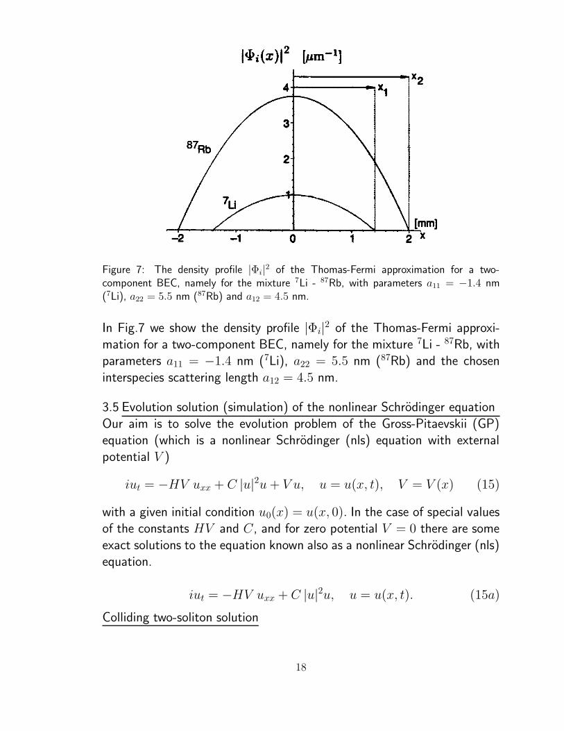
Figure 7: The density profile |Φi|2 of the Thomas-Fermi approximation for a two-component BEC, namely for the mixture 7Li - 87Rb, with parameters a11 = −1.4 nm(7Li), a22 = 5.5 nm (87Rb) and a12 = 4.5 nm.

In Fig.7 we show the density profile |Φi|2 of the Thomas-Fermi approxi-mation for a two-component BEC, namely for the mixture 7Li - 87Rb, withparameters a11 = −1.4 nm (7Li), a22 = 5.5 nm (87Rb) and the chosen

interspecies scattering length a12 = 4.5 nm.

3.5 Evolution solution (simulation) of the nonlinear Schrodinger equation

Our aim is to solve the evolution problem of the Gross-Pitaevskii (GP)equation (which is a nonlinear Schrodinger (nls) equation with external

potential V )

iut = −HV uxx + C |u|2u+ V u, u = u(x, t), V = V (x) (15)

with a given initial condition u0(x) = u(x, 0). In the case of special valuesof the constants HV and C, and for zero potential V = 0 there are some

exact solutions to the equation known also as a nonlinear Schrodinger (nls)equation.

iut = −HV uxx + C |u|2u, u = u(x, t). (15a)

Colliding two-soliton solution

18

Let us consider the following nls equation

iut = uxx + 2|u|2u (16)

which means that we use HV = −1, C = +2 and V = 0 in (15).Equation (16) admits the following (colliding) two-soliton solution:

u(x, t) =e−i(2x−20−3t)

cosh(x− 10 − 4t)+

e+i(2x+20−3t)

cosh(x+ 10 + 4t)(17)

Bright soliton solution

The most widely known soliton solution of the nls equation of the form

iut = −uxx − |u|2u (HV = 1, C = −1, V = 0) (18)

is the bright soliton. Its general form is the following:

u(x, t; a, c) = a ei( c2(x−ct)+nt)/ cosh(a(x− ct)/

√2) (19)

with the constraint a2 = 2(n−(

c2

)2) > 0.

If c = 1, n > 14. Let n = 5

4. Then a2 = 2, a =√

2. The bright solitonsolution is then

u(x, t;√

2, 1) =√

2ei( 1

2(x−t)+ 5

4t)/ cosh(x− t). (20)

The initial condition in this case is

u(x, 0;√

2, 1) =√

2eix/2/ cosh(x) (21a)

and the norm is (independent of t):∫

|u(x, t;√

2, 1)|2dx = 4. (21b)

In case of c = 2 we have the bright soliton

u(x, t;±2, 2) = ±2ei((x−2t)+3t)/ cosh(±√

2(x− 2t)), (22)

and the initial condition

u(x, 0;±2, 2) = ±2eix/ cosh(±√

2x). (22a)

Dark soliton solution

19

The nls equation

iut = −uxx + |u|2u (HV = 1, C = +1, V = 0) (23)

supports dark soliton solution of the form

u(x, t;m, c) = rei(Θ−mt), (23a)

with real amplitude r = r(x − ct), real phase Θ = Θ(x − ct), and realparameters c = const, m = const > c2/2 > 0 satisfying the relations

r2 = m− 2κ2/ cosh2(κ(x− ct))

and1/ tan(Θ) = −2κ tanh(κ(x− ct)).

In the course of testing the simulation program we shall use the dark soliton

solution with parameters m = 1, c = 1.Ma solitary wave solution

Equation

iut = −uxx − |u|2u (HV = 1, C = −1, V = 0) (24)

also has the Ma solitary wave solution of the form

u(x, t; a,m) = aeia2t[1 + 2m(m cosΘ + in sin Θ)/f(x, t)] (25)

with real parameters a and m and the following relations and definitions:

n2 = 1 +m2, Θ = 2mna2t, f(x, t) = n cosh(ma√

2x) + cos Θ.

In the course of testing the simulation program we shall use the Ma solitarywave solution with parameters a = 1,m = 1/2.

Rational-cum-oscillatory solutionEquation

iut = −uxx − |u|2u (HV = 1, C = −1, V = 0) (26)

also has the rational-cum-oscillatory solution of the form

u(x, t) = eit

[

1 − 4(1 + 2it)

1 + 2x2 + 4t2

]

(27).

Simulation procedure

20

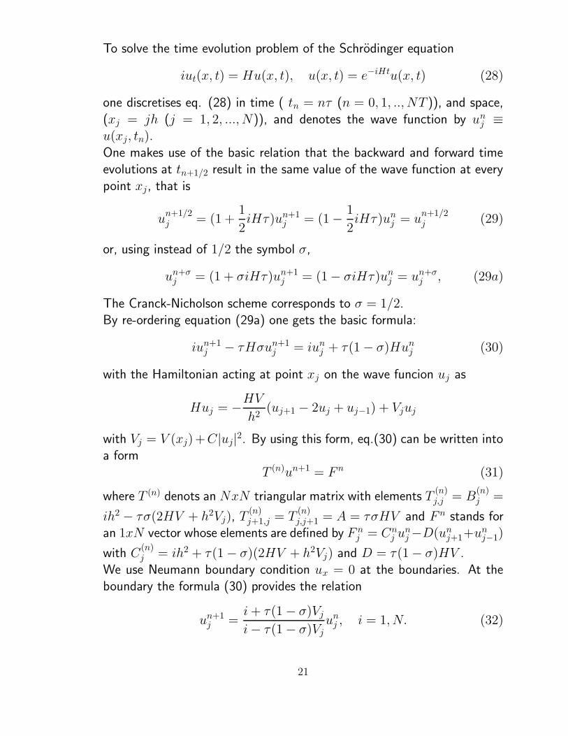
To solve the time evolution problem of the Schrodinger equation

iut(x, t) = Hu(x, t), u(x, t) = e−iHtu(x, t) (28)

one discretises eq. (28) in time ( tn = nτ (n = 0, 1, .., NT )), and space,

(xj = jh (j = 1, 2, ..., N)), and denotes the wave function by unj ≡

u(xj, tn).

One makes use of the basic relation that the backward and forward timeevolutions at tn+1/2 result in the same value of the wave function at every

point xj, that is

un+1/2j = (1 +

1

2iHτ)un+1

j = (1 − 1

2iHτ)un

j = un+1/2j (29)

or, using instead of 1/2 the symbol σ,

un+σj = (1 + σiHτ)un+1

j = (1 − σiHτ)unj = un+σ

j , (29a)

The Cranck-Nicholson scheme corresponds to σ = 1/2.By re-ordering equation (29a) one gets the basic formula:

iun+1j − τHσun+1

j = iunj + τ(1 − σ)Hun

j (30)

with the Hamiltonian acting at point xj on the wave funcion uj as

Huj = −HVh2

(uj+1 − 2uj + uj−1) + Vjuj

with Vj = V (xj)+C|uj|2. By using this form, eq.(30) can be written intoa form

T (n)un+1 = F n (31)

where T (n) denots an NxN triangular matrix with elements T(n)j,j = B

(n)j =

ih2 − τσ(2HV + h2Vj), T(n)j+1,j = T

(n)j,j+1 = A = τσHV and F n stands for

an 1xN vector whose elements are defined by F nj = Cn

j unj −D(un

j+1+unj−1)

with C(n)j = ih2 + τ(1 − σ)(2HV + h2Vj) and D = τ(1 − σ)HV .

We use Neumann boundary condition ux = 0 at the boundaries. At theboundary the formula (30) provides the relation

un+1j =

i+ τ(1 − σ)Vj

i− τ(1 − σ)Vjun

j , i = 1, N. (32)

21

colliding 2 solitons - exact

’s.dat’

-5

-4

-3

-2

-1

0

-20-15-10-505101520

0

0.5

1

1.5

2

t

x

|y(x,t)|

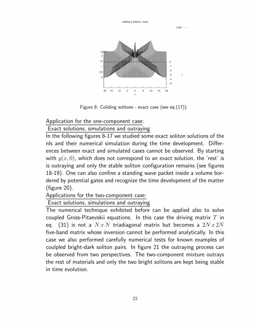
Figure 8: Coliding solitons - exact case (see eq.(17)).

Application for the one-component case:

Exact solutions, simulations and outrayingIn the following figures 8-17 we studied some exact soliton solutions of the

nls and their numerical simulation during the time development. Differ-ences between exact and simulated cases cannot be observed. By startingwith y(x, 0), which does not correspond to an exact solution, the ’rest’ is

is outraying and only the stable soliton configuration remains (see figures18-19). One can also confine a standing wave packet inside a volume bor-

dered by potential gates and recognize the time development of the matter(figure 20).

Applications for the two-component case:Exact solutions, simulations and outraying

The numerical technique exhibited before can be applied also to solvecoupled Gross-Pitaevskii equations. In this case the driving matrix T ineq. (31) is not a N xN triadiagonal matrix but becomes a 2N x 2N

five-band matrix whose inversion cannot be performed analytically. In thiscase we also performed carefully numerical tests for known examples of

coulpled bright-dark soliton pairs. In figure 21 the outraying process canbe observed from two perspectives. The two-component mixture outrays

the rest of materials and only the two bright solitons are kept being stablein time evolution.

22

bright - exact

’s.dat’

0

0.5

1

-15-10-5051015

0

0.5

1

1.5

2

t

x

|y(x,t)|

Figure 9: Brigth soliton - exact case (see eq.(19)).

bright -simulation

’y.dat’

0

0.5

1

-15-10-5051015

0

0.5

1

1.5

2

2.5

t

x

|y(x,t)|

Figure 10: Brigth soliton - simulation (see eq.(31)).

23

rational soliton - exact

’s.dat’

0

0.5

1

1.5

-10-5

05

10

00.5

11.5

22.5

3

t

x

|y(x,t)|

Figure 11: Brigth soliton - exact case (see eq.(22)).

rational soliton - simulation

’y.dat’

0

0.5

1

1.5

-10-5

05

10

00.5

11.5

22.5

3

t

x

|y(x,t)|

Figure 12: Brigth soliton - simulation (see eq.(31)).

24

dark - exact

’s.dat’

-1.5

-1

-0.5

0

-10-50510

0.70.750.8

0.850.9

0.951

t

x

|y(x,t)|

Figure 13: Dark soliton - exact case (see eq.(23a)).

dark - simulation

’y.dat’

-1.5

-1

-0.5

0

-10-50510

0.70.750.8

0.850.9

0.951

t

x

|y(x,t)|

Figure 14: Dark soliton - simulation (see eq.(31)).

25

Ma soliton - exact

’s.dat’

00.5

11.5

22.5

-10-5

05

10

00.5

11.5

22.5

33.5

t

x

|y(x,t)|

Figure 15: Ma solitary wave - exact case (see eq.(25)).

Ma soliton, y(1-10)=y(n-10) Neumann b.c.

’y.dat’

00.5

11.5

22.5

-10-5

05

10

00.5

11.5

22.5

33.5

t

x

|y(x,t)|

Figure 16: Ma solitary wave - simulation. Neumann b.c. used at j=1-10 and N-10 - N.(see eq.(32)).

26

Ma soliton, y(1)=y(n) Neumann b.c.

’y.dat’

00.5

11.5

22.5

-10-5

05

10

00.5

11.5

22.5

33.5

4

t

x

|y(x,t)|

Figure 17: Ma solitary wave - simulation. Neumann b.c. used at j=1 and N. (see eq.(32)).

outraying - bright remnant

’y.dat’

-5

-4

-3

-2

-1

0

-20-15-10-505101520

0

0.5

1

1.5

2

2.5

t

x

|y(x,t)|

Figure 18: By starting with initial condition y(x, 0) which does not correspond to an exactsolution the ’rest’ is is outraying and only the stable soliton configuration remains. Hereis shown one soliton.

27

outraying - 2-bright remnants

’y.dat’

-0.7-0.6-0.5-0.4-0.3-0.2-0.10

-20-15-10-505101520

0

0.5

1

1.5

t

x

|y(x,t)|

Figure 19: By starting with initial condition y(x, 0) which does not correspond to an exactsolution the ’rest’ is outraying and only the stable soliton configuration remains. Here areshown two solitons.

allo hullamcsomag bezarva ket fal koze

’y.dat’ 0.429 0.344 0.258 0.172

0.0859

-15

-10

-5

0-25 -20 -15 -10 -5 0 5 10 15 20 25

00.10.20.30.40.50.6

t

x

|y(x,t)|

Figure 20: Development of a standing wave packet within a closed interval of spacebordered by potential walls at x = −25 and x = 0 (not shown)

28

0

0.5

1

1.5

2

2.5-20 -15 -10 -5 0 5 10 15 20

012345678|y(x,t)|

’y1.dat’u 3:2:1’y2.dat’u 3:2:1

t

x

|y(x,t)|

00.511.522.5-20 -15 -10 -5 0 5 10 15 20

012345678

|y(x,t)| ’y1.dat’u 3:2:1’y2.dat’u 3:2:1

tx

|y(x,t)|

Figure 21: Outraying when a two-component mixture starts from a uniform density. Twostable solitons remain, the rest is outrayed . The process is exibited from two perspectives.

29