University of Kentucky University of Kentucky

UKnowledge UKnowledge

Theses and Dissertations--Electrical and Computer Engineering Electrical and Computer Engineering

2019

STUDY OF FACTORS AFFECTING DISTRIBUTION SYSTEM PV STUDY OF FACTORS AFFECTING DISTRIBUTION SYSTEM PV

HOSTING CAPACITY HOSTING CAPACITY

Fanxun Li University of Kentucky, fanxun821@gmail.com Digital Object Identifier: https://doi.org/10.13023/etd.2019.213

Right click to open a feedback form in a new tab to let us know how this document benefits you. Right click to open a feedback form in a new tab to let us know how this document benefits you.

Recommended Citation Recommended Citation Li, Fanxun, "STUDY OF FACTORS AFFECTING DISTRIBUTION SYSTEM PV HOSTING CAPACITY" (2019). Theses and Dissertations--Electrical and Computer Engineering. 140. https://uknowledge.uky.edu/ece_etds/140

This Master's Thesis is brought to you for free and open access by the Electrical and Computer Engineering at UKnowledge. It has been accepted for inclusion in Theses and Dissertations--Electrical and Computer Engineering by an authorized administrator of UKnowledge. For more information, please contact UKnowledge@lsv.uky.edu.

STUDENT AGREEMENT: STUDENT AGREEMENT:

I represent that my thesis or dissertation and abstract are my original work. Proper attribution

has been given to all outside sources. I understand that I am solely responsible for obtaining

any needed copyright permissions. I have obtained needed written permission statement(s)

from the owner(s) of each third-party copyrighted matter to be included in my work, allowing

electronic distribution (if such use is not permitted by the fair use doctrine) which will be

submitted to UKnowledge as Additional File.

I hereby grant to The University of Kentucky and its agents the irrevocable, non-exclusive, and

royalty-free license to archive and make accessible my work in whole or in part in all forms of

media, now or hereafter known. I agree that the document mentioned above may be made

available immediately for worldwide access unless an embargo applies.

I retain all other ownership rights to the copyright of my work. I also retain the right to use in

future works (such as articles or books) all or part of my work. I understand that I am free to

register the copyright to my work.

REVIEW, APPROVAL AND ACCEPTANCE REVIEW, APPROVAL AND ACCEPTANCE

The document mentioned above has been reviewed and accepted by the student’s advisor, on

behalf of the advisory committee, and by the Director of Graduate Studies (DGS), on behalf of

the program; we verify that this is the final, approved version of the student’s thesis including all

changes required by the advisory committee. The undersigned agree to abide by the statements

above.

Fanxun Li, Student

Dr. Yuan Liao, Major Professor

Dr. Aaron Cramer, Director of Graduate Studies

STUDYOF FACTORSAFFECTING DISTRIBUTION SYSTEM PV HOSTINGCAPACITY

THESIS

A thesis submitted in partial fulfillment of therequirements for the degree of Master of Science in Electrical Engineering

in the College of Engineeringat the University of Kentucky

By

Fanxun Li

Lexington, Kentucky

Director: Dr. Yuan Liao, Professor of Electrical and Computer Engineering

Lexington, Kentucky

2018

Copyright © Fanxun Li 2019

ABSTRACT OFTHESIS

STUDY OF FACTORS AFFECTING DISTRIBUTION SYSTEM PVHOSTING CAPACITY

As renewable energy plays an increasingly important role in the power system,

the addition of PV systems to the distribution network has become a major trend in

the current power system development. However, if a PV system with excessive

capacity is added to the distribution network, voltage problems may occur in the

system. Hence, it is important to determine the capacity of the PV system that can be

added at the distribution system.

The thesis aims to identify the major factors that affect the PV hosting capacity

of distribution systems. The thesis studies various scenarios for the IEEE-123 test

network PV system and evaluates the PV hosting capacity of the distribution system

based on simulation tools including Matlab and Opendss software.

KEYWORDS: Photovoltaic (PV) system, Hosting capacity, IEEE-123 test net ,

Opendss

Fanxun Li

05/13/2019

Date

STUDY OF FACTORS AFFECTING DISTRIBUTION SYSTEM PV HOSTINGCAPACITY

BY

Fanxun Li

Yuan Liao

(Director of Thesis)

Aaron Cramer

(Director of Graduate Studies)

5/13/2019

III

ACKNOWLEDGEMENTS

The following thesis is considered a personal work, but it cannot be completed

without the help of the following people. Special thanks are extended to my thesis

advisor, committee members, parents and friends. Without their help and support, I

couldn't have finished my work.

First of all, I would like to express my most sincere gratitude to professor Yuan

Liao, my thesis supervisor and chairman of the committee. He gave me detailed

guidance, which enabled me to increase my knowledge and learn research methods. I

would also like to thank my committee members, professor Himanshu Thapliyal and

professor Zhi Chen, for their valuable guidance and insights in my thesis defense.

In addition, I also want to thank my parents, who provided me with great

financial support for my study abroad. At the same time, I would like to thank my

friend Han Gao for his encouragement and help in the process of completing my

thesis, which made me more confident in my work.

IV

TABLE OF CONTENTS

ACKNOWLEDGEMENTS...................................................................................iii

TABLE OF CONTENTS........................................................................................iv

LIST OFTABLES...................................................................................................vi

LIST OF FIGURES..............................................................................................viii

Chapter 1 Introduction............................................................................. 1

1.1 Background.............................................................................................................. 1

1.2 Literature Review.....................................................................................................2

1.3 Thesis outline........................................................................................................... 7

Chapter 2 Components of PV System.................................................. 9

2.1 The structure of PV system...................................................................................... 9

2.2 The solar panels......................................................................................................10

2.3 The inverter............................................................................................................ 10

2.4 Hosting Capacity.................................................................................................... 12

Chapter 3 Software and experiment analysis.......................................14

3.1 Opendss introduction..............................................................................................14

3.2 Algorithm analysis................................................................................................. 17

Chapter 4 Case studies......................................................................... 20

4.1 Case A - PV placed at one bus.............................................................................20

4.2 Case B - PV placed at three chosen buses...........................................................30

V

4.3 Case C- Transformer tap adjust...........................................................................36

4.4 Case D The effect of reactive power injection on the maximum capacity of PVsystem...........................................................................................................................54

Chapter 5 Conclusions...........................................................................59

5.1 Summary of results obtained...............................................................................59

5.2 Conclusion..............................................................................................................60

5.3 Future work............................................................................................................ 61

Appendix.................................................................................................................. 62

References.................................................................................................67

Vita...........................................................................................................70

VI

LIST OFTABLES

Table 1 Initial transformer tap position information......................................... 19

Table 2 The PV system information..................................................................21

Table 3 PV system position and PV system capacity when the limiting voltage

is exceeded................................................................................................... 22

Table 4 Distance between each bus and substation bus, and values of resistance

and reactance................................................................................................ 28

Table 5 Grouping of random Numbers..............................................................32

Table 6 Three PV system location and the maximum PV capacity...................33

Table 7 The relationship between three physically adjacent buses and PV

capacity.........................................................................................................34

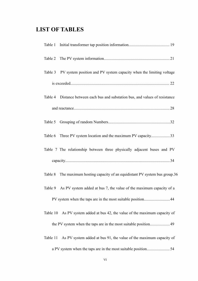
Table 8 The maximum hosting capacity of an equidistant PV system bus group.36

Table 9 As PV system added at bus 7, the value of the maximum capacity of a

PV system when the taps are in the most suitable position..........................44

Table 10 As PV system added at bus 42, the value of the maximum capacity of

the PV system when the taps are in the most suitable position....................49

Table 11 As PV system added at bus 91, the value of the maximum capacity of

a PV system when the taps are in the most suitable position....................... 54

VII

Table 12 The maximum allowable capacity of PV system when reactive power

is -500kw...................................................................................................... 56

Table 13 The maximum allowable capacity of PV system when reactive power

is -1000kw.................................................................................................... 57

VIII

LIST OF FIGURES

Figure 1 Structure of the PV system................................................................... 9

Figure 2 Schematic diagram of PV system....................................................... 12

Figure 3 Example of a COM. statement............................................................16

Figure 4 IEEE-123 test network........................................................................17

Figure 5 Chart of PV maximum capacity and node location............................ 27

Figure 6 Distance and PV capacity................................................................. 30

Figure 7 Relationship between the capacity and distance of three equidistantPV systems................................................................................................... 36

Figure- 8 The voltage variation for different tap positions of Tap 1a , with PVsystem added at bus 7...................................................................................39

Figure 9 The voltage variation for different tap positions of Tap3a , with PVsystem added at bus 7...................................................................................40

Figure 10 The voltage variation for different tap positions of Tap 4a , with PVsystem added at bus 7...................................................................................41

Figure 11 The voltage variation for different tap positions of Tap 4c , with PVsystem added at bus 7...................................................................................42

Figure 12 The voltage at each point when the tap position is most suitable.....43

Figure 13 The voltage variation for different tap positions of Tap 1a , with PVsystem added at bus 42.................................................................................45

Figure 14 The voltage variation for different tap positions of Tap 3a , with PVsystem added at bus 42.................................................................................46

Figure 15 The voltage variation for different tap positions of Tap 4a , with PVsystem added at bus 42.................................................................................47

Figure 16 The voltage variation for different tap positions of Tap 4c , with PVsystem added at bus 42.................................................................................48

Figure 17 The voltage at each point when the tap position is most suitable.....49

Figure 18 The voltage variation for different tap positions of Tap 1a , with PVsystem added at bus 91.................................................................................50

IX

Figure 19 The voltage variation for different tap positions of Tap 3a , with PVsystem added at bus 91.................................................................................51

Figure 20 The voltage variation for different tap positions of Tap 4a , with PVsystem added at bus 91.................................................................................52

Figure 21 The voltage variation for different tap positions of Tap 4c , with PVsystem added at bus 91.................................................................................53

Figure 22 The voltage at each point when the tap position is most suitable...54

1

Chapter 1 Introduction

1.1 Background

Countries around the world are paying more and more attention to

environmental protection and promoting energy conservation and emission reduction.

Wind power and photovoltaics are the cleanest energy sources are favored by the

world. Due to increased efficiency, decreasing cost and increased environmental

concern, photovoltaic installations have increased dramatically in recent years. The

feasibility of small-scale solar-based neighborhoods in urban areas has been

demonstrated in [1] and [2]. The same time PV system added in distribution system,

has led to new problems. That is the large-scale photovoltaic (PV) systems added at

the distribution network, will lead to over-voltage in the planning and operation of

the power distribution system. Once an over-voltage occurs, it often causes damage

to the equipment or even a large-scale power outage. Nowadays, how to increase the

capacity of PV system as much as possible under the premise of avoiding

over-voltage problem has attracted more and more attention.

Many companies provide a large number of interconnection requests

for new PV installations. As more PV nodes are built, the required

interconnections become tighter. For each PV node, the interconnection

shall be approved in time without affecting the reliability of the network.

Therefore, it is very important to understand the PV load capacity of the

network. Carrying capacity refers to the quantity of PV that can be

2

accommodated under the condition of existing control and infrastructure [3]

without affecting power quality or reliability.

Generally, the load hosting capacity of feeder in distribution line is determined

by the limit components and electrical constraints of distribution line, and the increase

of hosting capacity is observed by real-time information and dynamic performance

index calculation.

1.2 Literature Review

Some direct or indirect methods for observing hosting capacity are provided in

the following part of literature. In addition, some ideas are provided for the

experiment of this thesis.

Reference [4] presents a method combining automatic power factor with voltage

control is proposed to prevent the voltage of distribution system from continuing to

rise after reaching the limit. Simulation results show that DG hybrid voltage /PF

control can improve voltage distribution in weak networks, which is better than APFC

method. At the same time, the method also reduces the input and output reactive

power in the system, which also proves the effectiveness of the method.

Reference [5] performance of the power factor controller of the inverter interface

micro-source. The embedded low-voltage distribution network is simulated In the

PMCAD/EMTDC. By changing the frequency and operation mode of the system,

make sure that the controller can be very good regulation of the power factor makes it

match the system and proves that the controller can avoid the impact of small

3

interference on the system.

Reference [6] describes a distributed control strategy for photovoltaic units with

low cost and distributed energy. The strategy is simulated based on IEEE reference 13

bus feeder system. The simulation results show that this method can avoid the invert

caused by overvoltage at the power supply to a certain extent, and can also correct the

unit power factor of the system, providing many benefits for practical use.

Reference [7] describes some potential problems that may exist in solar PV

systems through EPRI and the use of advanced distribution system analysis tools

OPENDSS. The examples provided in this literature are helpful to evaluate the

hosting capacity of feeder PV and further analyze some characteristics of hosting

capacity through simulation. Then, by simulating the response, the feeder voltage

from each node of the substation to all endpoints is simulated, and it is proved that

with the increase of PV permeability, the deviation increases, and the increasing trend

is different for each feeder. As the voltage increases linearly, the PV space position

does help to adjust the deviation range of each feeder penetration level.

Reference [8] points out the problems faced by distribution engineers due to the

increase of distributed energy (DER), and points out that DER system needs different

mode adjustment in different regions. Lists some examples of the power factor and

inverter operation mode adjustment according to IEEE1547 equipment specification,

and has carried on the simulation, determine the IEEE1547 and NRECADG guidance

toolkit for DER distribution network security. Compared the PV inverter operation

4

under the voltage regulation mode to adjust the system voltage, and the common way

of adjusting unit power factor have different effects on the grid.

Reference [9] focuses on the volt/var power control of the inverter. Opendss

software was used to simulate the actual feeder model, and it was verified that the

inverter volt/var power control could provide sufficient support for the voltage change

caused by the output change caused by the addition of PV system, and the additional

feeder model was verified. Finally, the author points out that the extent to which

voltage/reactive power control supports the power grid is determined by hosting

capacity and PV location distribution.

References [10] considered the causes of voltage problems in large DER systems,

and analyzed the electrical characteristics of solar and wind energy systems. Through

the simulation of these two systems and the analysis of the results, this paper lists 10

standardization problems that should be paid attention to in the large-scale DER

system, and puts forward some processing and changes that should be taken by the

public utility to the system standardization.

References [11] discussed the PV penetration rate of distributed PV system and

single PV system. This model is established by comparing the average load

distribution of region 4 near the south gulf of Mexico and obtaining maximum hosting

capacity by changing the PV location information in the model in the subsequent

simulation. The results show the relationship between PV penetration trend and PV

position information.

5

Reference [12] is the first stage of the high photovoltaic osmosis project, mainly

to lay a foundation for subsequent projects, in order to better understand the impact of

high permeability of photovoltaic generators on the distribution system. The

establishment of this model involves various parameters of substation and PV board.

Then the seepage trend is analyzed by simulating the parameters and observing the

results. This paper mainly introduces the idea of observing the real trend change based

on the model.

Reference [13] analyzed the relationship between PV penetration rate and

reverse power flow in PV system. The data recorded by two PV devices are calculated

and analyzed, and the relationship between system efficiency and geographical

location is obtained. Subsequently, the IEEE 13 model was used for simulation

analysis to determine the voltage problem caused by the reverse power flow. It is

determined that the PV system will continue to supply local loads after the grid failure.

The greater the number of PV systems in the distribution network, the greater the

probability of island accidents.

Reference [14] used 96 houses in a Dutch community as a model to study the

interaction between PV systems and harmonic currents generated by ordinary

electronic loads. And a variety of scenarios are designed for simulation: single PV

system, single line PV system, linear load, PV system, nonlinear load. By observing

the simulation results, it is concluded that THD increases with the increase of

nonlinear load.

6

Reference [15] introduces GridLab-D simulation method, which is a new

modeling and simulation method of open power system. The operation method of

gridlab-d is introduced with wind turbine, housing and radial distribution system as

examples. The role of these capabilities in modernizing the power infrastructure was

affirmed. The PV system is added to the distribution network by this method.

Reference [16] uses the hypothetical illustrative feeder system as the model,

studies the capability of the voltage regulation method of the distribution network

with reverse current by generating various conditions, and compares the system

performance by using the coordinated control of inverter and public facilities. In the

simulation model, by changing the PV load capacity and position information for

simulation, it is concluded that the inverter can well change the voltage curve.

Reference [17] studied DSTATCOM's capability of reactive power compensation

for the system, which ensured that there was no over-voltage accident in the

distribution network under the maximum PV capacity. In the research process,

three-phase power flow analysis was carried out for the distribution network with PV

system added, and the substation feeder was selected for computer simulation so that

the distribution network obtained the maximum PV installation capacity. After that,

the lifetime of the entire distribution network and the benefits of adding PV systems

are calculated.

Reference [18] proposed a method to increase PV management capacity by

controlling capacitors, LTC, voltage regulators, controlled branch switches and

7

intelligent inverters to coordinate the use of ADNM. After that, the simulation was

completed on the IEEE123 bus test network, and the conditions of different PV

positions and different working power factors were studied. Simulation results show

that ADMN can significantly improve PV hosting capacity. In addition, ADNM can

help utilities quickly solve the voltage problem in their feeders.

Reference [19] studied how to realize reactive power control on the photovoltaic

inverter to adjust the photovoltaic hosting capacity of the distribution network. In

Matlab and Opendss, local Volt-Var droop control method is used for simulation, and

several practical unbalanced three-phase distribution feeders are studied. The results

show that this method can significantly improve PV hosting capability. The results

can meet the needs of utilities and researchers.

References [20] describe different dynamic requirements of German power grid.

And the FRT test procedure for executing PV inverter systems, and the method for

calculating power flow based on instantaneous values. The basic control structure of

inverter is systematically introduced. EMT simulation results are used to illustrate the

dynamic characteristics of the inverter in the process of grid disturbance. Three

examples in the simulation show that the inverter can meet the requirements of the

power grid.

1.3 Thesis outline

The structure of this thesis is as follows: Chapter 2 introduces the components of

the PV system, from the overall structure to the specific photovoltaic panels, inverters,

8

and also introduces the host capacity. Chapter 3 introduces the software and

experimental methods we use, and introduces the simulation network used in this

paper: the ieeee-123 test network. Chapter 4 is the specific process of the experiment,

which makes the results more intuitive by using images and tables. Chapter 5

summarizes all of the conclusions and presents the factors that affect the hosting

capability and how to increase the hosting capacity.

9

Chapter 2 Components of PV System

2.1 The structure of PV system

Photovoltaic (PV) systems are power systems designed to provide usable solar

energy through photovoltaic generation. According to the application form,

application scale and load type of solar photovoltaic system, it can be divided into the

following six types: small solar power generation system, simple dc system;

Large-scale solar power generation system, ac and dc power supply system, public

power grid connection; Hybrid power supply system, grid-connected system.

Typically, PV systems include the following components, solar panels, cables,

trackers, inverters, batteries, monitoring and metering systems. Figure 1 shows the

structure of the PV system.

Figure- 1 Structure of the PV system

2.2 The solar panels

Photoelectric conversion efficiency factor η % is an important factor for

10

evaluating the quality of solar panels. Photoelectric conversion efficiency factors

currently in use are normally: η=24% (solar cell laboratory) and vertical 15%

(industrial). The filling factor of FF % is an important factor to evaluate the load

capacity of solar cells.

)/()( mm ocsc VIVIFF (2.1)

Equation(2.1) represents the fill factor. mI is optimal working current, mV is

optimal working voltage SCI is short circuit current, OCV is open circuit voltage,

standard light intensity and ground environment temperature: AM=1.5 light intensity,

2m/1000W , t = 25°C. Temperature and light intensity will affect conversion

efficiency in some extent.

2.3 The inverter

The characteristics of the inverter are usually defined by the following four

factors:

1. Stable output voltage

For a qualified frequency converter, the steady-state output voltage shall not

exceed 5% of the rated value when the input voltage changes within the range of

10.8v~14.4v, and the output voltage deviation shall not exceed 10% of the rated value

when the load changes.

2. Waveform distortion of output voltage

For sinusoidal inverters, the maximum allowable waveform distortion (or

11

harmonic content) should not exceed 5% (single-phase output is 10%). If the

waveform distortion of the inverter is too large, a lot of heat energy will be generated

by the load elements, which is not conducive to the safety of electrical equipment and

seriously affects the operating efficiency of the system.

3. Load power factor

The ability of an inverter to carry an inductive or capacitive load. The load power

factor of sine wave inverter is 0.7 to 0.9, and the nominal value is 0.9. Under the

condition of constant load power, if the power factor of the inverter is low, the

capacity of the inverter needs to be increased, and the apparent power of the AC

circuit of the photovoltaic system will increase, resulting in the increase of loop

current, system loss ,and decrease system efficiency.

4. Inverter efficiency

The efficiency of inverter refers to the ratio of output power to input power under

specified working conditions. Normally, the nominal efficiency of PV inverter refers

to the pure resistance load, 80% load efficiency. At present, the nominal efficiency of

the mainstream inverter is between 80% and 95%, and the efficiency of the

low-power inverter should not be less than 85%.

2.4 Hosting Capacity

When a large amount of power output of the PV system flows on the line, it is

12

easy to generate voltage fluctuations or even exceed the limit. In addition, system

voltage fluctuations occur quickly and frequently when PV system output changes. At

present, it is difficult to adjust the voltage with the reactive power compensation

equipment of ordinary lines, so it is necessary to limit the capacity of the photovoltaic

system to a certain extent.

The influence principle of the PV system on node voltage is shown below.

Figure 2 shows a simplified PV system circuit model. Taking the substation bus

(equivalent system) as the balance node, the line transmission power is jQP , the

line impedance is jXR , the end load power is LjQLP , and the PV power supply

output is 00 jQP .

Figure- 2 Schematic diagram of PV system

After the PV power supply is connected, the line transmission power is：

0PPP L 0QQQ L (2.2)

Ignoring the transverse component of the voltage drop, the voltage loss on the

13

line is:

0VQXPRV

(2.3)

Where, R, X is the resistance and reactance of the distribution line. 0V is the

voltage on the feeder. The terminal voltage is the difference between the substation

bus voltage and the line loss voltage.

RQXVVV

P

00 *)(（2.4）

It can be seen from the above formula that the observation of voltage changes on

the line can infer whether the capacity of the PV system added meets the

requirements.

14

Chapter 3 Software and experiment analysis

3.1 Opendss introduction

Open Source Distribution System Simulator (Opendss for short) is an integrated

electrical system simulation tool for power distribution system [21]. Generally used to

analyze the following problems:

• Transformer frequency response analysis.

• Wind farm collector simulation.

• Wind farm impact on local transmission.

• Wind generation and other DG impact on switched capacitors and voltage

regulators.

• Development of DG models for the IEEE Radial Test Feeders.

It performs its analysis types in the frequency domain, it does NOT perform

electromagnetic transients (time domain) studies.

3.1.1 The use of Opendss

First, we need to find the latest official installer from this link:

Http://sourceforge.net/projects/electricdss/files/

After that, the installer is up and running. For starters, Opendss is a very friendly

piece of software. In the accompanying DOC file, you can learn many ways to use it,

15

which will get you through the early learning curve faster. In the Testcases file, there

are many models. By using the main file under each model, you can adjust the base

values of the model and adjust the model data to the values you want, and then run the

models in these files. In general, each model has two run files that you can select as

you wish. The results are generally divided into images and data.

You can close or open image results with the Opendssview statement. Opendss's

home page allows you to output individual results. If you only need a separate voltage

or current, use the display button on the page to select it. If you want to output the

overall result, you can do so by using the Ctrl + D shortcut. If you have a problem you

can't solve, discuss it with Opendss users at Sourceforge.

3.1.2 COM interface introduction

The COM interface allows the user to develop algorithms in another computer

program and then drive the OpenDSS engine to perform operations that are not

currently implemented in it. Good use of the COM interface is to write looping scripts

for programs in Opendss, because the scripting language in OpenDSS has no looping

capability. In general, users can use programs such as Matlab, C++, and Python to use

COM interfaces and write subroutines to adjust programs in Opendss to meet

expectations. Figure 3 is an example of using a COM interface tool.

16

Figure- 3 Example of a COM. statement

3.1.3 IEEE-123 test network introduction

The IEEE 123 node test network operates at a nominal voltage of 4.16kv. The

test network consists of overhead and underground lines, unbalanced loads, four

voltage regulators, parallel capacitor banks and multiple switches. In the state of

original data, the test network can provide constant current and the convergence

problem of power flow is minimal [23]. The impedance of the IEEE-123 test network

is determined by the basic data of the circuit, but it can be modified to meet the needs

of the user.

The network can be used to simulate various voltage problems that may occur in

the actual distribution network. The internal circuit of the test network is composed of

a mixture of single-phase, two-phase and three-phase lines. This thesis chose this

network mainly because its internal nodes are large enough to carry out a variety of

case analysis. Please refer to the attached table for the specific construction line code.

17

The Figure 4 shows the specific bus number in the line and the line connection.

Figure- 4 IEEE-123 test network

3.2 Algorithm analysis

In this paper, to analyze the hosting capacity, we added the PV system to the

IEEE-123 test network and gradually changed the PV capacity. The maximum allowable

capacity of the PV system was determined by observing the node voltage change caused by

changing PV capacity. In the analysis, PV injection of each phase was adopted for each node.

Therefore, PV injection of each phase was the same at the three-phase node of 4.16 KV,

which is equivalent to saying the three-phase PVsystem.

This papermainly studies the following three scenarios:

(1) Keep the transformer tap position to some initial value.

In this scenario, the state of all devices remains unchanged by default. Only the

position of the PV system and the capacity of the PV system are used as variables.

This scenario keeps the tap position of the transformer at an initial value and does not

18

change them during the simulation. It is also assumed that the PV system does not

provide or consume reactive power. Starting from the substation bus, the same PV

system is added to each bus one by one, and the PV capacity is gradually increased to

100kw when the PV system is added at a bus, and the maximum allowable capacity is

determined by observing the voltage simulation image. The relationship between PV

system capacity and the location is determined by comparing the results of these

maximum allowable capacities Set VV %105max .

In this scenario, we will conduct two case studies. The first one is that we only

add A PV system into the test network (case A). Through this experiment, we can see

the relationship between PV system location and maximum capacity. Next, three PV

systems will be added simultaneously to the test network (case B). In case B, we will

conduct a set of comparative experiments, and the specific experimental contents will

be explained later. Through this set of comparative experiments, we can find the

relationship between the number of PV system added and the maximum PV system

capacity allowed. Table 1 shows the initial position of the transformer tap. By

disabling the transformer control function in OpenDSS, we keep the tap position of

the transformer unchanged.

19

Table 1 Initial transformer tap position information

Name Tap Min Max Step Position

reg1a 1.025 0.9 1.1 0.00625 4

reg2a 1.0125 0.9 1.1 0.00625 2

reg3a 1 0.9 1.1 0.00625 0

reg3c 1.00625 0.9 1.1 0.00625 1

reg4a 1.05 0.9 1.1 0.00625 8

reg4b 1.025 0.9 1.1 0.00625 4

reg4c 1.03125 0.9 1.1 0.00625 5

(2) Adjust transformer tap position and keep PV system position unchanged.

In this scenario, the PV system added is the same as the PV system added in

scenario 1, except the capacity is different. We kept the PV system in the same

position at the bus and conducted experiments by adjusting the tap position of the

transformer. The IEEE-123 test network has four transformers and seven transformer

taps. We will reasonably select several taps for simulation, and distinguish and adjust

the positions of several taps, and determine the maximum allowable hosting capacity

by observing the change of voltage. This scenario is called Case C.

(3) Consider the reactive power input from the PV system.

In previous experiments, the PV system was defaulting without reactive power

injection. In this scenario, reactive power injection is taken as an influencing factor.

Two experiments were set, and reactive power Q=-500 and Q=-1000 were

respectively set in the two experiments. The maximum allowable PV system capacity

20

was determined by observing the voltage. The results were compared with Case A to

observe the impact of reactive power of the PV system on capacity.

21

Chapter 4 Case studies

4.1 Case A - PV placed at one bus

In Case A, we add one PV system in the test network, one by one. we put the PV

system information in Table 2:

Table 2 The PV system information.

Irradiance: Set the present irradiance value in kW/sq-m. Used as the base value

for shape multipliers. Generally entered as peak value for the time period of interest

and the yearly, daily, and duty load shape objects are defined as per unit

multipliers.[22]

Pmpp: Set the rated max power of the PV array for 1.0 kW/sq-m irradiance and a

user-selected array temperature.[22]

PF: Nominally, the power factor for the output power. Default is 1.0. Setting this

property will cause the inverter to operate in CONSTANT POWER FACTOR MODE.

Enter negative when kW and kvar have opposite signs. [22]

We simulated the IEEE-123 test network with a PV system in Matlab through the

COM interface. The PV capacity range is set to 0KW to 10000KW, and the PV

system is added one by one at the substation bus to the last bus. Check the results and

record the PV capacity when all voltages exceed the limit voltage, and record all

voltage irradiance Pmpp PF mode Kva(min) Kva(max)

4.16kv 1.0 10000 1 daily 100kw 10000kw

22

results in Table 3.

Table 3 PV system position and PV system capacity when the limiting voltage is

exceeded

PV location voltage(KV) The node PV capacity(KW)

1 No No No

2 1.05 12 10000

3 1.0504 8 4500

4 1.0502 6 4500

5 1.0503 10 2600

6 1.0505 9 2600

7 0.94998 2 6600

8 0.94998 2 6200

9 0.94979 46 8600

10 0.94982 15 6200

11 0.94982 15 6200

12 1.0502 65 6400

13 1.05 66 2100

14 0.948 15 6600

15 1.0503 23 4200

16 1.0501 21 4400

17 1.0502 21 4400

18 1.0501 18 6000

23

19 1.0505 24 6500

20 1.0502 26 3900

21 1.0505 38 4900

22 1.0501 12 5800

23 1.0501 29 3400

24 1.0502 24 3600

25 1.0501 38 3400

26 1.0519 29 2700

27 1.0515 29 2500

28 1.0505 33 3100

29 1.0508 38 2900

30 1.0502 38 2500

31 1.0505 26 3700

32 1.0505 26 3700

33 1.0502 29 2700

34 1.0504 31 4900

35 1.0501 45 3300

36 1.503 42 2700

37 1.0512 44 4100

38 1.0504 46 1700

39 1.0502 45 1600

40 1.0503 49 2900

41 1.0502 49 1700

24

42 1.0504 49 1900

43 1.0503 45 2700

44 1.0502 49 2300

45 1.0503 51 5000

46 1.0508 53 3600

47 1.0507 52 2500

48 1.0501 49 2400

49 1.0506 55 2400

50 1.0501 56 2000

51 1.0501 57 2600

52 1.0504 59 5700

53 1.0503 60 5500

54 1.0502 61 4800

55 1.0505 62 3700

56 1.05 64 2800

57 1.0503 61 3800

58 1.0504 67 1800

59 1.0503 65 1800

60 1.0505 66 3300

61 1.0505 68 2300

62 1.0502 70 2200

63 1.0506 71 1900

64 1.0507 71 1400

25

65 1.0522 72 1100

66 1.0523 73 900

67 1.0501 66 3100

68 1.0506 75 4700

69 1.0507 78 2000

70 1.0509 80 1300

71 1.0524 81 1200

72 1.0505 100 2100

73 1.0503 83 1000

74 1.0513 84 600

75 1.0513 83 500

76 1.0508 100 1800

77 1.0501 93 400

78 1.0503 93 400

79 1.0503 93 400

80 1.0503 91 400

81 1.0501 93 300

82 1.0507 93 300

83 1.0514 93 200

84 1.0516 93 1500

85 1.0514 92 800

86 1.0504 100 800

87 1.0509 100 600

26

88 1.0502 93 900

89 1.0508 100 500

90 1,0511 93 1100

91 1.0505 100 500

92 1.0504 98 1200

93 1.0504 100 500

94 1.0516 102 900

95 1.0502 100 500

96 1.0512 93 1100

97 1.0501 66 3300

99 1.0508 107 1800

100 1.0503 107 1000

101 1.0506 110 2600

102 1.0510 115 2400

103 1.0525 114 1800

104 1.0521 113 1800

105 1.0506 112 2700

106 1.0508 93 1200

107 1.0512 93 1700

108 1.0504 116 2300

109 1.0523 118 1700

110 1.0509 120 1300

111 1.0509 120 1300

27

112 1.0507 120 1300

113 1.0532 123 1000

114 1.0524 124 900

After we have this table, in order to more clearly show the maximum capacity of

each bus. We set up Figure 5 with X-axis as the bus number where the PV is located,

and Y-axis as the PV capacity.

Figure- 5 Chart of PV maximum capacity and node location

To illustrate the relationship between PV capacity and distance, we recorded the

distance, resistance, and reactance of all nodes. Put all the information together to

build Table 4.

28

Table 4 Distance between each bus and substation bus, and values of resistance andreactance.

nodeDistance

(mi)

Resistance

(ohm)

Reactance

(ohm)node

Distance

(mi)

Resistance

(ohm)

Reactance

(ohm)

150r

149(S)0 0 0 61 0.573 0.01034265 0.088861413

1 0 0 0 62 0.573 0.01034265 0.088861413

2 0.076 0.0013718 0.011786156 63 0.621 0.01120905 0.096305301

3 0.076 0.0013718 0.011786156 64 0.654 0.0118047 0.101422974

4 0.123 0.00222015 0.019074963 65 0.72 0.012996 0.11165832

5 0.123 0.00222015 0.019074963 66 0.8 0.01444 0.1240648

6 0.185 0.00333925 0.028689985 67 0.574 0.0103607 0.089016494

7 0.076 0.0013718 0.011786156 68 0.64 0.011552 0.09925184

8 0.133 0.00240065 0.020625773 69 0.678 0.0122379 0.105144918

9 0.17 0.0030685 0.02636377 70 0.73 0.0131765 0.11320913

10 0.293 0.00528865 0.045438733 71 0.792 0.0142956 0.122824152

11 0.293 0.00528865 0.045438733 72 0.64 0.011552 0.09925184

12 0.17 0.0030685 0.02636377 73 0.692 0.0124906 0.107316052

13 0.17 0.0030685 0.02636377 74 0.744 0.0134292 0.115380264

14 0.213 0.00384465 0.033032253 75 0.811 0.01463855 0.125770691

15 0.256 0.0046208 0.039700736 76 0.692 0.0124906 0.107316052

16 0.275 0.00496375 0.042647275 77 0.73 0.0131765 0.11320913

17 0.275 0.00496375 0.042647275 78 0.806 0.0145483 0.124995286

18 0.227 0.00409735 0.035203387 79 0.825 0.01489125 0.127941825

19 0.383 0.00691315 0.059396023 80 0.825 0.01489125 0.127941825

20 0.431 0.00777955 0.066839911 81 0.915 0.01651575 0.141899115

21 0.383 0.00691315 0.059396023 82 0.948 0.0171114 0.147016788

29

22 0.44 0.007942 0.06823564 83 0.995 0.01795975 0.154305595

23 0.44 0.007942 0.06823564 84 0.948 0.0171114 0.147016788

24 0.487 0.00879035 0.075524447 85 1.076 0.0194218 0.166867156

25 0.487 0.00879035 0.075524447 86 0.73 0.0131765 0.11320913

26 0.606 0.0109383 0.093979086 87 0.863 0.01557715 0.133834903

27 0.658 0.0118769 0.102043298 88 0.948 0.0171114 0.147016788

28 0.54 0.009747 0.08374374 89 0.948 0.0171114 0.147016788

29 0.577 0.01041485 0.089481737 90 1 0.01805 0.155081

30 0.634 0.0114437 0.098321354 91 1 0.01805 0.155081

31 0.606 0.0109383 0.093979086 92 1.042 0.0188081 0.161594402

32 0.648 0.0116964 0.100492488 93 1.042 0.0188081 0.161594402

33 0.658 0.0118769 0.102043298 94 1.085 0.01958425 0.168262885

34 0.227 0.00409735 0.035203387 95 1.085 0.01958425 0.168262885

35 0.455 0.00821275 0.070561855 96 1.142 0.0206131 0.177102502

36 0.455 0.00821275 0.070561855 97 0.64 0.011552 0.09925184

37 0.578 0.0104329 0.089636818 99 0.74 0.013357 0.11475994

38 0.578 0.0104329 0.089636818 100 0.844 0.0152342 0.130888364

39 0.625 0.01128125 0.096925625 101 0.688 0.0124184 0.106695728

40 0.455 0.00821275 0.070561855 102 0.735 0.01326675 0.113984535

41 0.502 0.0090611 0.077850662 103 0.778 0.0140429 0.120653018

42 0.502 0.0090611 0.077850662 104 0.84 0.015162 0.13026804

43 0.55 0.0099275 0.08529455 105 0.735 0.01326675 0.113984535

44 0.55 0.0099275 0.08529455 106 0.788 0.0142234 0.122203828

45 0.588 0.0106134 0.091187628 107 0.83 0.0149815 0.12871723

46 0.625 0.01128125 0.096925625 108 0.788 0.0142234 0.122203828

47 0.588 0.0106134 0.091187628 109 0.849 0.01532445 0.131663769

30

48 0.635 0.01146175 0.098476435 110 0.934 0.0168587 0.144845654

49 0.635 0.01146175 0.098476435 111 0.991 0.01788755 0.153685271

50 0.682 0.0123101 0.105765242 112 0.991 0.01788755 0.153685271

51 0.729 0.01315845 0.113054049 113 1.015 0.01832075 0.157407215

52 0.228 0.0041154 0.035358468 114 1.114 0.0201077 0.172760234

53 0.304 0.0054872 0.047144624 115（61s） 0.677 0.01221985 0.104989837

54 0.341 0.00615505 0.052882621 116（135s） 0.383 0.00691315 0.059396023

55 0.365 0.00658825 0.056604565 117（152s） 0.227 0.00409735 0.035203387

56 0.417 0.00752685 0.064668777 118（160s） 0.573 0.01034265 0.088861413

57 0.365 0.00658825 0.056604565 119（151s） 0.777 0.01402485 0.120497937

58 0.431 0.00777955 0.066839911 120（197s） 0.688 0.0124184 0.106695728

59 0.479 0.00864595 0.074283799 121（300s） 0.849 0.01532445 0.131663769

60 0.431 0.00777955 0.066839911

Integrate the information in Table 3 and Table 4.We took the distance from the

substation bus as the X-axis and the maximum capacity of a PV system as the Y-axis,

and created the chart and added the trend line for it. See in Figure 6.

Figure- 6 Relationship between Distance and PV capacity

31

As can be seen from Figure 6, the maximum PV capacity allowed to be added by

the distribution network and the distance from the bus to the substation bus basically

show a linear downward trend. As can be seen from Table 4, the values of resistance

and reactance are proportional to the distance. Therefore, it can be inferred that the

maximum PV system capacity allowed to be added in the distribution network is

related to the values of resistance and reactance of the distribution network lines.

4.2 Case B - PV placed at three chosen buses

In this case, three PV generations are added at three buses. We will study three

general cases. In the first case, we will put three PV generations at three randomly

chosen buses, and each bus has equal PV generation. In the second case, we choose

three physically adjacent buses to install the PV generations. In the third case, the

three buses are chosen such that each bus has an equal distance with the substation

bus.

4.2.1 PV placed at three randomly chosen buses

This case, we added three PV system in the IEEE-123 test network. The location

of these three PV system was randomly selected. Matlab function

round(rand(1,3)*130) is used to generate a random number group. Put all those

random number sets in Table 5.

32

Table 5 Grouping of random Numbers

Casenumber

1 2 3 4 5 6 7 8 9 10

Bus A 55 99 85 4 13 57 103 49 18 99

Bus B 89 97 22 36 17 50 24 74 19 97

Bus C 18 88 51 92 6 4 100 90 71 88

Casenumber

11 12 13 14 15 16 17 18 19 20

Bus A 26 62 76 76 7 113 20 64 32 83

Bus B 33 46 71 60 64 16 96 20 79 85

Bus C 45 80 108 40 9 94 41 38 73 94

In Table 5, Bus A, B, and C represent the selected three nodes, and the Case

number is the serial number of the experiment. The 20th group of data was not

generated randomly. Three nodes were selected from Table 3, that is, the node where

the minimum value of the maximum PV capacity allowed to be added in the

distribution network is located. After the simulation, the results are recorded in Table

6.

33

Table 6 Three PV system location and the maximum PV capacity.

PV location Max voltage(kv) Node Max capacity(kw)

55 89 18 1.0501 100 1500

99 97 88 1.0511 100 2000

85 22 51 1.0528 92 2100

4 36 92 1.0508 98 3000

13 17 6 1.0505 9 4700

57 50 4 1.0505 56 12700

103 24 100 1.0532 114 4000

49 74 90 1.053 65 2000

18 19 71 1.0515 80 2400

99 97 88 1.0511 100 2000

26 33 45 1.0502 29 4800

62 46 80 1.0503 93 1200

76 71 108 1.0523 80 2300

76 60 40 1.0516 44 4800

7 64 9 1.0505 71 8700

103 16 94 1.0501 100 2700

20 96 41 1.0508 93 3000

64 20 38 1.0502 26 4300

32 79 73 1.0508 65 2500

83 85 94 1.0504 92 1000

As can be seen from the Table 6, when the three nodes added by the PV system

are in different positions, there is a large gap between these maximum capacities of

the PV system. However, there was no significant correlation. Random selection of

nodes results in a random change of PV system capacity.

34

4.2.2 Three physically adjacent buses to install the PV generations.

This thesis assumes that the maximum capacity of the PV system is related to the

position of the three buses connected by the PV system. In this case, we selected 10

groups of buses adjacent to each other through Figure 4. Three PV systems are added

at these buses and the maximum allowable PV system capacity under such

circumstances is compared to determine whether the maximum PV capacity will

change as a result. The summary of the results is placed in Table 7.

Table 7 The relationship between three physically adjacent buses and PV capacity.

PV location Max voltage（kv) Node number Max capacity(kw)

3 5 6 1.0513 8 4800

15 16 34 1.0509 69 6900

42 44 47 1.0518 49 2400

52 53 54 1.0505 61 5900

57 58 59 1.0528 63 5800

68 69 70 1.0528 79 2400

76 77 78 1.0511 93 700

89 91 93 1.0501 100 500

102 103 104 1.051 115 2400

108 109 110 1.0552 120 2100

Comparing the results with Table 3 in case A, we found that adding a PV system

at three adjacent buses at the same time would affect the overall PV capacity.

However, the effect of the increase was not significant, and in the case of the seventh

set of data, it resulted in a decrease in the maximum PV capacity.

When you want to add a high-capacity PV system to a distribution network, you

35

can actually do this by breaking a large PV system into smaller PV systems and then

putting them into the distribution network. In this way, the over-voltage problem

caused by excessive PV capacity can be reduced in the distribution network. This

method is more suitable when the selected bus is located in the middle of the

distribution network.

4.2.3 The three buses are chosen such that each bus has an equal distance with

the substation bus.

It can be inferred from the above experiments that the maximum allowable

capacity of the PV system added in the distribution network is related to the distance

from the bus added to the substation bus. In this experiment, 10 groups of buses are

selected from Table 4 of Case A. Among these 10 groups, the distance between each

bus in each group and the substation bus is almost the same, but the substation bus

distance between each group is different. In this way, the variables are limited.

Through this set of experiments, the influence of the maximum allowable capacity of

the PV system can be studied by adding the number of PV systems in the distribution

network. The maximum capacity of the PV system is recorded in Table 8 through

simulation.

36

Table 8 The maximum hosting capacity of an equidistant PV system bus group.

PV Capacity Distance MaxVoltage(KV)

Node Maxcapacity(KW)

2 3 7 0.076 1.0426 12 23000

9 12 13 0.17 1.0502 13 14700

18 34 52 0.227 1.0504 27 12900

19 21 55 0.383 1.0506 24 8600

35 36 40 0.455 1.0517 42 2700

30 48 49 0.635 1.0508 55 3000

68 72 97 0.64 1.0513 100 4300

27 33 64 0.658 1.0523 29 3600

70 77 86 0.73 1.0502 93 1800

82 88 89 0.948 1.0516 93 800

To make this more intuitive, take the distance as the X-axis and the maximum

capacity as the Y-axis.Build the chart and add the trend lines, as shown in Figure 7.

Figure- 7 Relationship between the capacity and distance of three equidistant PVsystems

37

It can be seen from the Figure 7 that whether the PV system is added at three

equidistant buses at the same time, or the PV system is added at a single bus, the

maximum PV capacity will gradually decrease as the distance increases. By

comparing these 10 sets of results with Case A, it can be found that the closer the

distance from the substation bus is, the larger the total capacity of the three added PV

systems will be, and the total capacity will decrease when the distance is close to 1

mile. It can also be inferred that the maximum PV system capacity allowed to be

added at the distribution network does not vary much depending on the number of PV

systems added.

4.3 Case C- Transformer tap adjust.

In this case, we will continuously adjust the tap position of the transformer and

compare the results to determine whether the change of tap position of the transformer

will affect the maximum capacity of the PV system added at the distribution network.

In the IEEE-123 test network, there are four transformers and seven taps in total.

The tap position is adjusted several times and the voltage changes of each bus in the

distribution network are recorded during each adjustment. Use charts to compare the

results of each simulation to make the presentation clear.

We will choose three three-phase buses 7,42,91 for simulation. The three buses

were chosen because they are at different distances from the substation bus. The bus 7

is less than 0.1mi, bus 42 is about 0.5mi, and bus 91 is about 1mi. The three

three-phase buses are also selected to reduce the disturbance term, so the only variable

38

is the tap position.

In order to reduce the impact of other variables on the results, the taps selected

are the same for each adjustment. We will conduct four experiments for each selected

bus. The selected taps to be adjusted are 1a, 3a, 4a, and 4c, and only one tap is

adjusted per test. Each transformer in this system has 33 tap positions (one "rated" tap

in the center, 16 for increasing and decreasing turns), allowing ±10% transformer

voltage variation (0.625% variation per step) from the rated transformer rating, which

in turn allows for step voltage regulation of the output.

The 2a tap is not selected because it is mounted on the 2a transformer, which is

mounted on bus 9, bus 9r on a single-phase line. For the selected bus, no matter how

the 2a tap is adjusted, the line voltage will not be affected. Therefore, no analysis is

performed here.

At first, we added the PV system at the bus 7, the capacity of this PV system is

6600 KW, and the data is from Table 4.Figure 8 shows the change in line voltage each

time the tap 1a is adjusted. The uppermost horizontal red line indicates the voltage

limit(± 5% maxV ), and the three colors the black, the red and the blue respectively

indicate the a, b, and c phases in the three phases. The six images respectively indicate

that the tap 1a is placed at six positions of -4, 0, 4, 8, 12 and 16.

Figure 9 shows the voltage change in each time the tap 3a, Figure 10 and Figure

11 shows the change of tap 4a and tap 4c.

39

Figure- 8 The voltage variation for different tap positions of Tap 1a , with PV systemadded at bus 7

40

Figure- 9 The voltage variation for different tap positions of Tap3a , with PV systemadded at bus 7

41

Figure- 10 The voltage variation for different tap positions of Tap 4a , with PV systemadded at bus 7

42

Figure- 11 The voltage variation for different tap positions of Tap 4c , with PV systemadded at bus 7

43

From the above chart analysis, it can be seen that when the PV system is added

at the bus 7, the appropriate adjustment range of the tap 1a is located at (-2, 8). The 3a

tap has no effect on the overall voltage, mainly because of the No. 3 transformer is

located on the two-phase line. The tap 4a, 4c adjust the voltages of the two phases a

and c, and the appropriate ranges are at (-4, 8) and (-4, 6), respectively. Figure 12

shows the voltage of the system when all the taps are adjusted to the most appropriate

state. The position of each tap and the maximum PV system capacity are shown in

Table 9.

L-N Voltage Profile

0.00 0.50 1.00 1.50Distance (km)

0.960

0.980

1.000

1.020

1.040

p.u. Voltage

Figure- 12 The voltage at each point when the tap position is most suitable

44

Table 9 As PV system added at bus 7, the value of the maximum capacity of a

PV system when the taps are in the most suitable position.

Tap name Tap position Tap value PV max capacity(kw)

1a -2 0.9875

2a 2 1.0125

3a 0 1

500003c 1 1.00625

4a 8 1.05

4b 4 1.025

4c 6 1.0375

Next, the 40,91 bus was analyzed in the same way. Figure 13, Figure 14, Figure

15 and Figure 16,represents 4 charts of 40 bus. Figure 17 shows the voltage of the

system when all the taps are adjusted to the most appropriate state.

Figure 18, Figure 19, Figure 20 and Figure 21, represents 4 charts of 91 bus.

Figure 22 shows the voltage of the system when all the taps are adjusted to the most

appropriate state.

The position of each tap and the PV capacity are shown in Table 10 and Table 11.

45

Figure- 13 The voltage variation for different tap positions of Tap 1a , with PV systemadded at bus 42.

46

Figure- 14 The voltage variation for different tap positions of Tap 3a , with PV systemadded at bus 42.

47

Figure- 15 The voltage variation for different tap positions of Tap 4a , with PV systemadded at bus 42.

48

Figure- 16 The voltage variation for different tap positions of Tap 4c , with PV systemadded at bus 42.

49

L-N Voltage Profile

0.00 0.50 1.00 1.50Distance (km)

0.960

0.980

1.000

1.020

1.040

p.u. Voltage

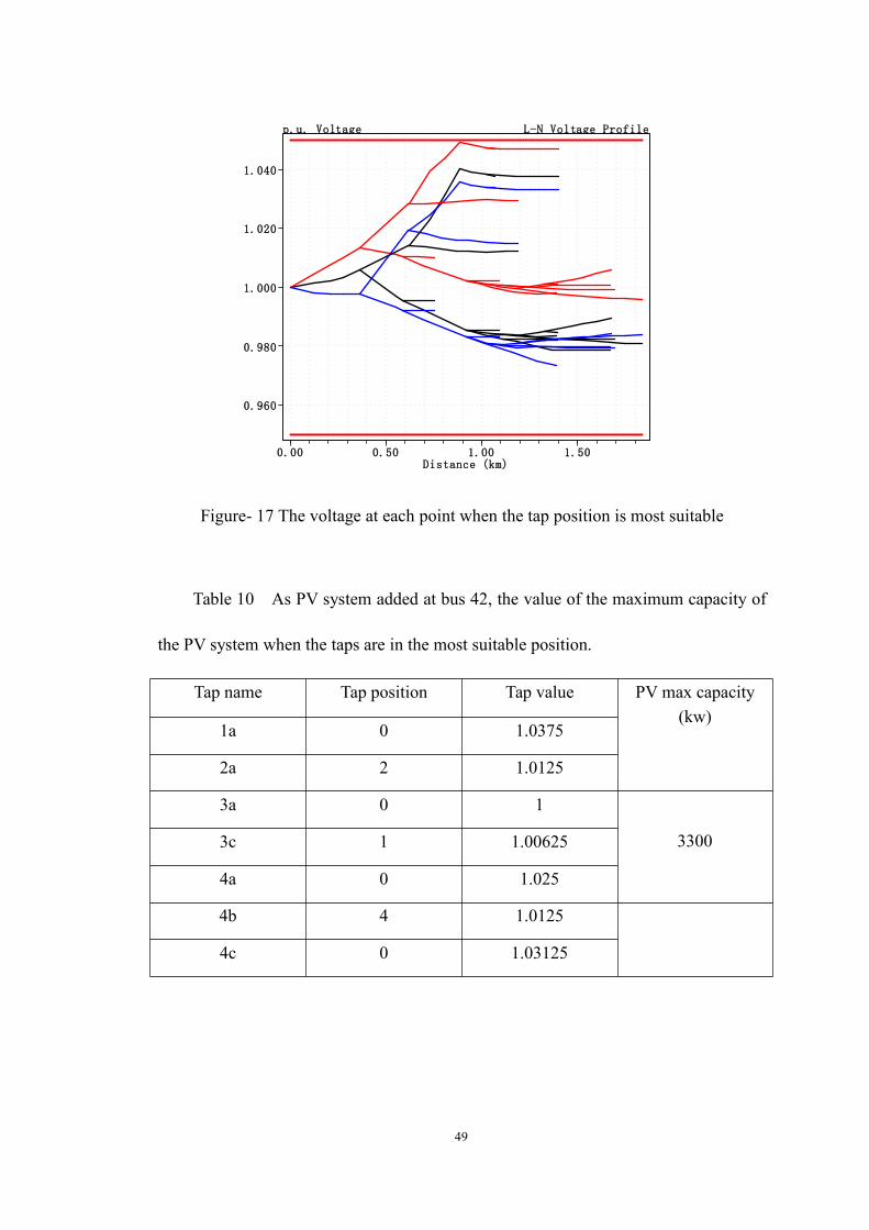
Figure- 17 The voltage at each point when the tap position is most suitable

Table 10 As PV system added at bus 42, the value of the maximum capacity of

the PV system when the taps are in the most suitable position.

Tap name Tap position Tap value PV max capacity(kw)

1a 0 1.0375

2a 2 1.0125

3a 0 1

33003c 1 1.00625

4a 0 1.025

4b 4 1.0125

4c 0 1.03125

50

Figure- 18 The voltage variation for different tap positions of Tap 1a , with PV systemadded at bus 91

51

Figure- 19 The voltage variation for different tap positions of Tap 3a , with PV systemadded at bus 91

52

Figure- 20 The voltage variation for different tap positions of Tap 4a , with PV systemadded at bus 91

53

Figure- 21 The voltage variation for different tap positions of Tap 4c , with PV systemadded at bus 91

54

L-N Voltage Profile

0.00 0.50 1.00 1.50Distance (km)

0.960

0.980

1.000

1.020

1.040

p.u. Voltage

Figure- 22 The voltage at each point when the tap position is most suitable

Table 11 As PV system added at bus 91, the value of the maximum capacity of

a PV system when the taps are in the most suitable position.

Tap name Tap position Tap value PV max capacity(kw)

1a 0 1

2a 2 1.0125

3a 0 1

40003c 1 1.00625

4a 4 1.025

4b 0 1

4c 4 1.025

From the above case, we can find that adjusting the transformer tap is indeed the

55

most effective way to increase the hosting capacity of the PV system. This is mainly

because the adjustment of the transformer tap is the reason for directly adjusting the

voltage. Comparing 41 and 91 bus, it can be found that under the influence of tap

adjustment, the distance from the substation bus is no longer the primary factor

affecting the hosting capacity, and the influence of the distance from the transformer

becomes the main influencing factor.

4.4 Case D The effect of reactive power injection on the

maximum capacity of PV system.

In this experiment, 20 nodes were selected to add a PV system. First, the reactive

power of the PV system was set to -500Kvar, and then adjusted to -1000kwKvar.

The two groups of experimental results were compared with the results of Case A to

determine the impact of reactive power on the maximum allowable capacity of the

PV system. The result respectively shows in Table 12 and Table 13.

56

Table 12 The maximum allowable capacity of PV system when reactive power is -500kw.

PV location Voltage(KV) Node PV capacity(KW)

17 1.0504 65 6200

19 1.0502 24 7300

25 1.0503 30 3700

28 1.0502 39 3300

31 1.0505 27 3100

34 1.0503 12 5900

37 1.0505 44 5700

43 1.0501 45 4600

45 1.0503 47 5500

49 1.0506 55 2600

55 1.0502 62 3800

61 1.0501 68 2700

67 1.0502 100 3600

73 1.0501 65 900

75 1.0504 83 800

77 1.0502 93 1200

79 1.0503 93 900

85 1.0517 92 1800

91 1.0503 100 800

103 1.0517 114 2400

57

Table 13 The maximum allowable capacity of PV system when reactive power is -1000kw.

PV location Voltage(KV) Node PV capacity(KW)

17 1.0501 12 5300

19 1.0506 47 6800

25 1.0502 30 3900

28 1.0504 38 3800

31 1.0506 27 2700

34 1.0503 12 5400

37 1.0508 47 4900

43 1.0512 48 5000

45 1.0502 47 4400

49 1.0507 55 2500

55 1.0505 62 4200

61 1.0501 68 3000

67 1.0502 68 4000

73 1.0507 67 800

75 1.0501 65 800

77 1.0501 92 1400

79 1.0511 92 1400

85 1.0504 98 700

91 1.0509 100 1200

103 1.0501 65 2400

Compared with Case A, we can see that the maximum capacity of the PV system

increases when reactive power injection is considered, and the extent of growth is

related to the value of reactive power. By comparing the two results of this

58

experiment, it can be seen that for each node, the allowable injected reactive power

has a unique upper limit, When the injected power exceeds the upper limit, the

reactive power impact the efficiency on the generator, cause the voltage drop, the

maximum allowable capacity of PV system will decrease.

59

Chapter 5 Conclusions

5.1 Summary of results obtained.

In the previous chapter, the use of Opendss is briefly introduced, and the factors

affecting the hosting capacity of PV system added at the distribution network are

studied. We mainly built the model in Opendss by adding PV system at the test

network of IEEE-123, then analyzed the model in Matlab through COM interface, and

finally input the analysis results into EXCEL for data analysis. In this thesis, there are

6 experiments, 3 independent experiments, and 3 comparative experiments.

First, A separate PV system was added at the IEEE-123 test network in Case A to

prove that the distance from the substation bus has an impact on hosting capacity.

Then in Case B, whether the number of the PV system added at the distribution

network will influence the maximum capacity of the PV system is determined by

changing the connection of the number of PV systems. This case is tested under three

random conditions, physically adjacent an equal distance. The experiment shows that

the PV system connected by the group is more helpful for voltage stability of

distribution network than that connected with the large-scale PV system. Finally, by

changing the position of the transformer tap proved that the total hosting capacity of

the PV system was different for each bus at different tap positions. The distance

between the bus and the transformer would affect the extent to which the adjusting tap

affected the maximum capacity of the PV system.

60

5.2 Conclusion.

Nowadays, the world's demand for energy is gradually increasing, and the

demand for renewable energy is also increasing. Distributed generation, which makes

efficient use of local resources, has thus become more and more popular. As important

renewable energy resources, photovoltaic (PV) systems are much valued in today's

environment. Integrating PV into the grid may cause system performance problems

such as overvoltage and protection mis-coordination. This thesis focuses on

overvoltage problem. This thesis aims to examine the factors that affect the maximum

hosting capacity of a PV system, so as to propose some methods to increase the

hosting capacity of the PV system.

The studies in this thesis have shown that the distance between the bus and the

substation bus is one of the main factors affecting the hosting capacity of the PV

system added in the distribution network. As the distance increases, the maximum

capacity of the PV system that is allowable to be added at the distribution network

will gradually decrease. The total capacity of a group of PV systems added at

different locations in distribution network is larger than adding PV at a single

location. Compared with the total capacity of PV systems added at adjacent buses,

the total capacity of PV systems added at buses with the same distance is larger. The

adjustment of the tap has great impact on the hosting capacity of the PV system.

While adjusting the tap, the effects on the PV system capacity of the distance

between the bus containing the PV system and substation bus decrease. The effects

on the PV system caused by the distance between the bus and the transformer which

61

contains the tap will increase. We also consider the reactive power withdrawn by the

PV system from the distribution network. The maximum PV system capacity

allowed by the distribution network will increase when PV system consumes

reactive power, but each node has a maximum allowable reactive power limit.

In order to add a PV system with large enough capacity at the distribution

network and to avoid over-voltage problem, we can first divide the large capacity PV

system into multiple sets of PV generation systems of smaller capacity. Then we

place them at different locations in the distribution network. We try to place the PV

system close to the substation bus if possible while also considering voltage

regulator locations.

5.3 Future work.

This thesis examines several factors that affect the allowable capacity of PV

systems added at the distribution network. However, some aspects have not been

studied. In the future work, we can study the following aspects: the number and

location of the capacitor bank added to the distribution network, the opening and

closing state of the switches, and the single-phase and multi-phase PV systems.

62

Appendix

MATLAB CASE CODE%The IEEE123 distribution network example is used to calculate the three-phasecurrent by calling OpenDSS.

k=100;%PV system capacity from 100kva to k*100kva

Uo_kva=zeros(k,130);%In the k-th power flow calculation result, the A-phasevoltage standard value result .130 represents a total of 130 nodes (including switches)of the system.

for i=1:k %i is the range of PV system capacity changes, from 100kva to 2500kva

[DSSStartOK, DSSObj, DSSText] = DSSStartup; % Execute DSSStartup.m

if DSSStartOK

DSSText.command='Compile (C:\Users\79231\Desktop\论文

\OpenDSS\IEEETestCases\123Bus\IEEE123Master.dss)';

DSSCircuit=DSSObj.ActiveCircuit; % Set the variables of thematlab interface

DSSSolution=DSSCircuit.Solution;

%Add energy measuring components to measure the distance from the feeder tothe generator

DSSText.Command='New EnergyMeter.Main Line.SW1 1';

%Add another monitor

DSSText.Command='New Monitor.FeederEnd Line.L99 1';

% In order to get better calculation results, the limited adjuster tap adjusts onegear at a time.

% Use the COM interface's Regcontrols collection interface instead of thecommand interface to get the trend results and

% for power flow calculation

% Specify a variable in the RegControls interface

Regulators = DSSCircuit.RegControls;

%Loop all the regulators, from First to Next, etc.

iReg = Regulators.First;

while iReg>0

Regulators.MaxTapChange = 1;

63

Regulators.Delay = 30; % set all delays to 30s

iReg = Regulators.Next;

end

% Increase photovoltaic power

DSSText.Command ='New XYCurve.MyPvsT npts=4 xarray=[0 25 75 100]yarray=[1.2 1.0 0.8 0.6]';

DSSText.Command ='New XYCurve.MyEff npts=4 xarray=[0.1 0.2 0.4 1.0]yarray=[0.86 0.9 0.93 0.97]';

str=PVKva(i);

DSSText.Command =str;

%Set the trend calculation method

DSSText.Command = 'Solve Mode=snapshot';

%DSSText.Command = 'set mode=daily';

%DSSText.Command = 'set stepsize=1h';

DSSText.Command = 'set number=1';

% for m=1:5

% DSSSolution.Solve;

% end

if DSSSolution.Converged

a = ['Current calculation will converge in 'num2str(DSSSolution.Iterations) ' times'];

else

a = 'Trend results do not converge';

end

disp(a)

%Collect power and voltage results from power flow calculations

DSSText.Command = 'Export Elempowers';% Get the power calculationpower value

PowerFilename = DSSText.Result;

DSSText.Command = 'Export voltages';

VoltageFileName = DSSText.Result;

64

MyCSV = csvread(VoltageFileName,1, 1);

Volts = MyCSV(:,5); %Store the voltage value calculated by this powerflow in Volts

for j=1:130

Uo_kva(i,j)=Volts(j);

end

end

End

OPENDSS CODE~clear all

Compile (IEEE123Master.dss)

Set Opendssview=False

Transformer.reg1a.wdg=2 Tap=(0.00625 4 * 1 +)

Transformer.reg2a.wdg=2 Tap=(0.00625 2 * 1 +)

Transformer.reg3a.wdg=2 Tap=(0.00625 0 * 1 +)

Transformer.reg3c.wdg=2 Tap=(0.00625 1 * 1 +)

Transformer.reg4a.wdg=2 Tap=(0.00625 8 * 1 +)

Transformer.reg4b.wdg=2 Tap=(0.00625 4 * 1 +)

Transformer.reg4c.wdg=2 Tap=(0.00625 5 * 1 +)

RegControl.creg1a.maxtapchange=0 !Fixed at present tap

RegControl.creg2a.maxtapchange=0 !Fixed at present tap

RegControl.creg3a.maxtapchange=0 !Fixed at present tap

RegControl.creg4a.maxtapchange=0 !Fixed at present tap

RegControl.creg3c.maxtapchange=0 !Fixed at present tap

RegControl.creg4b.maxtapchange=0 !Fixed at present tap

RegControl.creg4c.maxtapchange=0 !Fixed at present tap

65

New EnergyMeter.Feeder Line.L115 1

solve

Buscoords Buscoords.dat ! load in bus coordinates

// add pv

New XYCurve.MyPvsT npts=4 xarray=[0 25 75 100] yarray=[1.2 1.0 0.8 0.6]

New XYCurve.MyEff npts=4 xarray=[0.1 0.2 0.4 1.0] yarray=[0.86 0.9 0.93 0.97]

! define PV

New PVSystem.PV1 phases=3 bus1=91 kV=4.16 kVA=500 irrad=1 Pmpp=10000

~ temperature=25 PF=1 effcurve=Myeff P-TCurve=MyPvsT

set mode=daily

set stepsize=1h

set number=24

solve

Plot Profile

Show Voltage LN Nodes

Show taps

plot Loadshape Object=default

DSSTART UPCODE

function [Start,Obj,Text] = DSSStartup

% Function for starting up the DSS

%instantiate the DSS Object

Obj = actxserver('OpenDSSEngine.DSS');

%

%Start the DSS. Only needs to be executed the first time w/in a

%Matlab session

66

Start = Obj.Start(0);

% Define the text interface

Text = Obj.Text;

67

REFERENCES

[1] Invited book chapter, Yuan Liao, Power Management and Protection of

Distribution Systems with Distributed Generations in book Handbook of Distributed

Generation, Springer International Publishing AG, Cham, Switzerland, 2017.

[2]Wen Fan and Yuan Liao, “Fault identification and location for distribution

network with distributed generations,” the International Journal of Emerging Electric

Power Systems, May 2018.S. Cobben, B. Gaiddon, and H. Laukamp,

WP4—Deliverable 4.3—Im-pact of Photovoltaic Generation on Power Quality in

UrbanAreasWith High PV Population EIE/05/171/SI2.420208, 2008.

[3]D. N. Gaonkar, P. C. Rao, and R. N. Patel, “Hybrid method for voltage

regulation of distribution system with maximum utilization of connected distributed

generation source,” in Proc. IEEE Power India Conf., 2006, p. 5.

[4]A. H. Rafa, O. Anaya-Lara, and J. R. McDonald, “Power factor control for

inverter-interfaced microgeneration,” in Proc. 43rd Int. Universities Power

Engineering Conf. 2008 (UPEC 2008), 2008, pp. 1–5.

[5] J. Seuss and R. G. Harley, "A low-cost distributed control strategy for rooftop PV

with utility benefits," in Power and Energy Society General Meeting (PES), 2013

IEEE, 2013, pp. 1-5.

[6] J. W. Smith, R. Dugan, M. Rylander, and T. Key, "Advanced distribution

planning tools for high penetration PV deployment," in Power and Energy Society

68

General Meeting, 2012 IEEE, 2012, pp. 1-7.

[7]G. J. Shirek and B. A. Lassiter, "Solar plant modeling impacts on distribution

systems PV case study," in IEEE Rural Electric Power Conference (REPC), 2012.

[8] J. Smith, W. Sunderman, R. Dugan, B. Seal, “Smart Inverter Volt/Var Control

Functions for High Penetration of PV on Distribution Systems,” IEEE Power

Systems Conference and Expo, March, 2011.

[9]S. J. Steffel, “Distribution Grid Considerations for Large Scale Solar and Wind

Installations,” IEEE PES 2010 Transmission and Distribution Conference

Proceedings, New Orleans, LA, April, 2010.

[10]A. Hoke, R. Butler, J. Hambrick, and B. Kroposki, "Steady-State Analysis of

Maximum Photovoltaic Penetration Levels on Typical Distribution Feeders," IEEE

Transactions on Sustainable Energy, 2012.

[11]J. Hambrick and D. Narang, “High-penetration PV deployment in the Arizona

public service system, phase 1 update,” in Proc. 2012 IEEE Photovoltaic Specialists

Conf., Austin, TX, June, 2012.

[12]V. Ramachandran, “Steady state analysis of three phase unbalanced distribution

systems with interconnection of photovoltaic cells,” in Proc. IEEE Power Systems

Conf. and Exposition, Phoenix, AZ, March.2011.

[13]M. C. Benhabib, J. M. A. Myrzik, and J. L. Duarte, “Harmonic effects caused by

large scale PV installations in LV network,” presented at the Int. Conf. Electrical

69

Power Quality and Utilization, Barcelona, Spain, October, 2007, 6 pages.

[14]K. Schneider, D. Chassin, Y. Pratt, and J. C. Fuller, “Distribution power flow for

smart grid technologies,” in Proc. IEEE/PES Power Systems Conf. and Exposition,

Seattle, WA, March, 2009, pp. 1–7.

[15]Y. Liu, J. Bebic, B. Kroposki, J. de Bedout, andW. Ren, “Distribution system

voltage performance analysis for high-penetration PV,” in Proc. IEEE Energy 2030

Conf., Atlanta, GA, November, 2008, pp. 1–8.

[16]Chao-Shun Chen ; Chia-Hung Lin, Wei-Lin Hsieh, Cheng-Ting Hsu, Te-Tien

Ku “Enhancement of PV Penetration With DSTATCOM in Taipower Distribution

System,” IEEE Transactions on Power Systems, May 2013, Vol.28(2),

pp.1560-1567.

[17]Ding, Fei, Mather, Barry, “On Distributed PV Hosting Capacity Estimation,

Sensitivity Study, and Improvement,” IEEE Transactions on Sustainable Energy,

2017, Vol.8(3).

[18]J. Seuss, M. J. Reno, R. J. Broderick, and S. Grijalva, “Improving distribution

network PV hosting capacity via smart inverter reactive power support,” in Proc.

2015 IEEE PES General Meeting, Jul. 2015, pp. 1–5.

[19]T. Neumann, I. Erlich, "Modelling and control of photovoltaic inverter systems

with respect to German grid code requirements," in Power and Energy Society

General Meeting, 2012 IEEE, 2012, pp. 1-8.

70

[20]Program Revision: 7.6. September 2012. Page 1 of 35. New User Primer. The

Open Distribution System Simulator™.

[21] R.C. Dugan, Reference Guide. The Open Distribution System Simulator

(OpenDSS), EPRI, July, 2010.

[22] K. P. Schneider, B. A. Mather, B. C. Pal, C. W. Ten, G. J. Shirek, H. Zhu, J. C.

Fuller, J. L. R. Pereira, L. F. Ochoa, L. R. de Araujo, R. C. Dugan, S. Matthias, S.

Paudyal, T. E. McDermott, and W Kersting, “Analytic Considerations and Design

Basis for the IEEE Distribution Test Feeders,” IEEE Transactions on Power Systems,

vol. PP, no. 99, pp. 1-1, 2017.

71

VITA

Education

08/2017— 05/2019

Master Student

Department of Electrical and Computer Engineering, University of Kentucky,Lexington, Kentucky, USA

09/2013—06/2017

Bachelor of Engineering

Electrical Engineering and Automation, North China Electric Power University,China

Awards

25/07/2016-26/08/2016

Won first prize in the project research about shortening the debugging andnetworking time of the county network integration system during the internship in theNational Network of Shenyang Yuhong Power Supply Company awarded byShenyang Quality Association, Shenyang Federation of Trade Unions and ShenyangWomen’s Federation

06/2014

Won the third prize in the Debate contest in North China Electric PowerUniversity

09/2013

Obtained the honorable title of “the advanced individual” awarded by NorthChina Electric Power University