Page 1
Study on Linking a
SuperCritical Water-Cooled Nuclear Reactor to a
Hydrogen Production Facility
By
Andrew John Lukomski
A Thesis Submitted in Partial Fulfillment
of the Requirements for the Degree of
Master of Applied Science
Nuclear Engineering
The Faculty of Energy Systems and Nuclear Science
University of Ontario Institute of Technology
July 2011
© Andrew Lukomski, 2011
Page 2
ii
ABSTRACT
The SuperCritical Water-cooled nuclear Reactor (SCWR) is one of six Generation-IV
nuclear-reactor concepts currently being designed. It will operate at pressures of 25 MPa
and temperatures up to 625°C. These operating conditions make a SuperCritical Water
(SCW) Nuclear Power Plant (NPP) suitable to support thermochemical-based hydrogen
production via co-generation. The Copper-Chlorine (Cu‒Cl) cycle is a prospective
thermochemical cycle with a maximum temperature requirement of ~530°C and could be
linked to an SCW NPP through a piping network. An intermediate Heat eXchanger (HX)
is considered as a medium for heat transfer with operating fluids selected to be SCW and
SuperHeated Steam (SHS). Thermalhydraulic calculations based on an iterative energy
balance procedure are performed for counter-flow double-pipe design concept HXs
integrated at several locations on an SCW NPP coolant loop. Using various test cases,
design and operating parameters are recommended for detailed future research. In
addition, predicted effects of heat transfer enhancement on HX parameters are evaluated
considering theoretical improvements from helically-corrugated HX piping. The effects
of operating fluid pressure drop are briefly discussed for applicability in future studies.
Keywords: Hydrogen Production, Thermochemical Cycles, Copper-Chlorine Cycle,
Generation IV Reactor, SuperCritical Water-cooled nuclear Reactor, Heat Exchanger
Page 3
iii
ACKNOWLEDGEMENTS
Many individuals enabled me to carry out this research and complete my academic
studies. I would like to thank my whole family, especially my parents, Janina and
Mieczyslaw, who were a source of continuous support and advice. Their faith provided
encouragement to move forward, especially during periods of struggle. I would like to
extend thanks to friends who supported me throughout this work and to fellow students
and researchers who helped overcome challenges during these studies, your support was
always appreciated: Lisa Grande, Wargha Peiman, Dr. Zhaolin Wang,
Dr. Venkata Daggupati, Harwinder Thind, Sarah Mokry and Eugene Saltanov. Thank
you to past professors, teachers and others who have shared their knowledge and
experiences over the years. To all of the support staff at UOIT who assisted with this
thesis, I am appreciative of your efforts and the time you dedicated to support its
completion. Finally, to my supervisors, Dr. Kamiel Gabriel and Dr. Igor Pioro, I
sincerely thank you for the guidance you provided throughout my studies. Your support
extended beyond the academic and contributed to my personal development.
Generous financial support from NSERC/NRCan/AECL Generation IV Energy
Technologies Program, ORF and NSERC Discovery Grants are gratefully acknowledged
in support of this work.
Page 4
iv
SUMMARY
Various alternatives for hydrogen production are being considered to reduce the demand
on fossil fuel-based production methods. Thermochemical cycles are one alternative
which generate hydrogen through the decomposition of water using reactions of
intermediate materials and the input of thermal energy. The Copper-Chlorine (Cu‒Cl)
cycle requires temperatures of approximately 530°C to enable hydrogen production.
There are several variations of this cycle, however, discussion is limited to the 5 and
4-step cycles. The 4-step cycle was primarily considered in this investigation based on
ongoing research at the hydrogen research facility at the University of Ontario Institute of
Technology (UOIT). By providing a source of non-fossil fuel-based thermal energy to
the Cu‒Cl cycle, a more environmentally sustainable method of hydrogen production can
be achieved.
One of the energy sources considered for the Cu‒Cl cycle is the SuperCritical Water-
cooled nuclear Reactor (SCWR). The SCWR is a Generation IV nuclear reactor concept
that would operate with SuperCritical light Water (SCW) coolant at pressures of 25 MPa
and reactor outlet temperatures up to 625°C. There are several Nuclear Power Plant
(NPP) cycles which an SCWR could be designed to, two of which are discussed in this
investigation: the no-reheat and single reheat cycles. In theory, the SCWR could provide
the thermal energy requirements for the Cu‒Cl cycle via a Heat eXchanger (HX) linking
the two facilities. An intermediate loop of SuperHeated Steam (SHS) would be heated in
the HX and deliver the thermal energy to the Cu‒Cl reactors.
The objective of this research is to provide a review of recent development in the Cu‒Cl
cycle and SCW NPP concepts, identify preliminary design and operating parameters for
an interfacing HX and perform thermalhydraulic calculations to determine suitable
designs for future development. A counter-flow double-pipe HX design is selected as the
choice HX due to the feasibility of performing iterative calculations across individual HX
pipes. An HX integrated downstream of the SCWR (termed “HX A”) in the no-reheat
cycle layout would have SCW flow in the inner pipe and SHS in the annulus gap. In the
Page 5
v
single reheat cycle, one HX could be located identically as in the no-reheat layout or in a
different location, downstream of the SCWR reheat channels (termed “HX B”). This
second HX would operate with SHS flowing in both the inner pipe (High Pressure fluid ‒
HP) and annulus gap (Low Pressure fluid ‒ LP).
A multi-purpose MATLAB script was developed to perform thermalhydraulic
calculations based on iterative energy balances for the HXs at locations on the two NPP
cycles. The code allows thermal approximations to be tested based on the Log Mean
Temperature Difference (LMTD) method. In addition, frictional pressure losses for both
flows can be calculated across the HX pipe lengths. User input parameters include SHS
(for HX A)/LP SHS (for HX B) operating pressure and pipe mass flow rates, SCW (for
HX A)/HP SHS (for HX B) pipe mass fluxes, and inner and outer piping dimensions.
Three piping materials (Inconel‒600, Inconel‒718 and Stainless Steel 304) were
evaluated for mechanical properties including burst pressure and thermal conductivity to
assess the feasibility of their use in the topic HXs. A lower bounding analysis was
selected using SS‒304 as the piping material. A number of combinations were developed
based on the user inputs and then evaluated for heat transfer characteristics,
thermophysical properties and other parameters such as flow velocity. For HX A, 26
suitable combinations were identified for further development. For HX B, 5 suitable
combinations were determined with operating parameters documented. Profiles of
thermophysical properties, fluid temperature and pressure drop were prepared for a select
number of combinations. The effects of theoretical heat transfer enhancement were
evaluated and concluded that significant reductions in HX heat transfer area may be
realized with 75% increase in local Heat Transfer Coefficients (HTC). Results obtained
from the MATLAB code were verified through a reproduction of the code in Microsoft
Excel with a comparison between sample results.
The study concludes that an HX at either of the locations investigated may supply the
thermal energy requirements of the Cu‒Cl cycle. Furthermore, in terms of HX A, none
of the proposed operating conditions permitted the SCW temperature to exit the HX
Page 6
vi
below the pseudocritical temperature at 25 MPa. This will require a suitable SCW re-
entry point to the NPP coolant loop to be established. More detailed pressure loss
calculations will be required in future work which will further refine suitable operating
and design parameter combinations.
Page 7
vii
TABLE OF CONTENTS
INTRODUCTION .............................................................................................................. 1
CHAPTER 1 – HYDROGEN PRODUCTION .................................................................. 3
1.1 COPPER-CHLORINE CYCLE ........................................................................... 5
CHAPTER 2 – GENERATION IV NUCLEAR REACTOR DESIGNS ......................... 12
CHAPTER 3 – SUPERCRITICAL WATER AND HEAT TRANSFER
CORRELATIONS ............................................................................................................ 19
3.1 Heat Transfer Correlations ................................................................................. 22
3.1.1 Heat Transfer Correlations for SHS ............................................................ 22
3.1.2 Heat Transfer Correlations for SCW .......................................................... 23
CHAPTER 4 –SELECT SCW NUCLEAR POWER PLANT LAYOUTS AND
COGENERATION HEAT EXCHANGERS .................................................................... 26
4.1 No-Reheat Cycle Layout .................................................................................... 29
4.2 Single-Reheat Layout ......................................................................................... 31
4.3 Selection of Heat Exchanger Design and Preliminary Analysis ........................ 34
4.4 Log Mean Temperature Difference Method ...................................................... 36
4.5 Heat Exchanger Piping Material ........................................................................ 37
4.6 Heat Transfer Enhancement ............................................................................... 41
CHAPTER 5 – THERMALHYDRAULIC CALCULATIONS ....................................... 44
5.1 Assumptions ....................................................................................................... 45
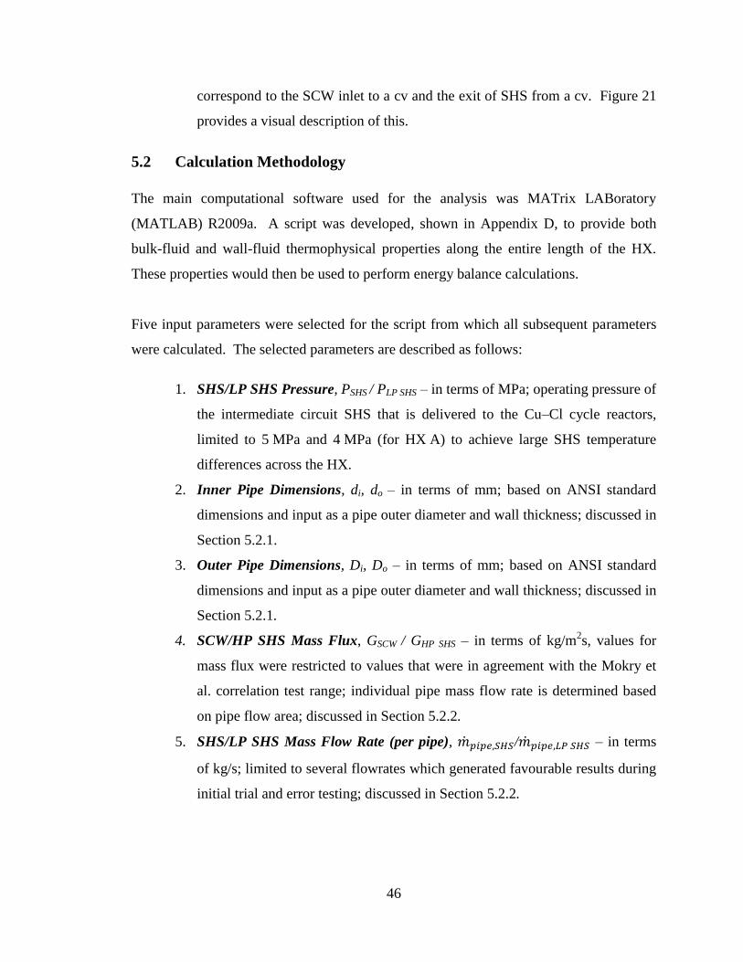
5.2 Calculation Methodology ................................................................................... 46
5.2.1 Piping Dimensions ...................................................................................... 48
5.2.2 Temperature Calculations ........................................................................... 51
5.2.3 MATLAB Code Verification ...................................................................... 59
5.2.4 Pressure Drop Calculation .......................................................................... 60
CHAPTER 6 – RESULTS AND DISCUSSION .............................................................. 62
6.1 Results for HX A (SCW/SHS) Design ............................................................... 62
6.2 Results for HX B (HP SHS/LP SHS) Design .................................................... 76
Page 8
viii
CHAPTER 7 – CONCLUSIONS ..................................................................................... 83
CHAPTER 8 – FUTURE WORK .................................................................................... 87
REFERENCES ................................................................................................................. 88
APPENDIX A – RESULTS TABLES ........................................................................... A1
APPENDIX B – CODE VERIFICATION ................................................................... A10
APPENDIX C – SUMMARY OF CALCULATION STEPS ...................................... A16
APPENDIX D – MATLAB SCRIPT ........................................................................... A19
APPENDIX E – PUBLICATIONS .............................................................................. A49
APPENDIX F – CONFERENCES .............................................................................. A50
Page 9
ix
LIST OF FIGURES
Figure i1. (a) Pressure-Temperature Diagram for Water; (b) Temperature and Heat
Transfer Coefficient Profiles Along Heated Length of Vertical Circular Tube: Water,
D=10 mm and L=4 m. (Pioro et al., 2011). ...................................................................... xix
Figure 1. Conceptual Cu–Cl Cycle Layout Based on a 5-Step Process (adapted from
Naterer et al., 2008; Lukomski et al., 2010b). .................................................................... 9
Figure 2. Conceptual Layout for the 4-Step Cu‒Cl Cycle (adapted from Naterer et al.,
2010). ................................................................................................................................ 11
Figure 3. World-wide Status of Currently Operating Nuclear Reactors (PRIS, 2011). .... 12
Figure 4. Evolution of Nuclear Reactor Designs (Generation IV Forum, 2008). ............. 14
Figure 5. Pressure-Temperature Diagram of Water with Typical Operating Conditions of
SCWRs, PWR, CANDU‒6 and BWR (Pioro and Duffey, 2007). ................................... 17
Figure 6. General Concept of Pressure-Tube SCW CANDU Reactor: IP-Intermediate-
Pressure Turbine, and LP-Low-Pressure Turbine (Pioro and Duffey, 2007). ................. 17
Figure 7. Schematic of US Pressurized-vessel SCW Nuclear Reactor (Pioro and Duffey,
2007). ................................................................................................................................ 18
Figure 8. Dependency of the Specific Heat of Water on Temperature and Pressure (NIST,
2010). ................................................................................................................................ 20
Figure 9. Peak Specific Heat Values of Water at Pseudocritical Points (NIST, 2010). ... 20
Figure 10. Select Thermophysical Properties of Water in the Pseudocritical Region at 25
MPa (NIST, 2010). ........................................................................................................... 21
Figure 11. Potential Intermediate SHS Network Inside of a Hydrogen Production Facility.
........................................................................................................................................... 28
Figure 12. No-Reheat Cycle Layout for a SCW NPP ....................................................... 30
Figure 13. Heat Exchanger Locations in the No-Reheat Cycle SCW NPP Layout
(Lukomski et al., 2011c). .................................................................................................. 30
Figure 14. Cross Section of a Single Reheat PT SCWR Core for 1200 MWel NPP ........ 32
Figure 15. Single Reheat Cycle Layout for a SCW NPP .................................................. 33
Figure 16. Heat Exchanger Locations in the Single Reheat Cycle NPP Layout .............. 33
Figure 17. Variation of Tensile Strength for SS‒304 (Hendrix Group), Inconel‒600
(Annealed, Hot-Rolled Rod) (Special Metals, 2011), Inconel‒718 (Hot-Rolled Round,
Annealed and Aged 4-in Diameter Rod) (Special Metals, 2011). .................................... 39
Page 10
x
Figure 18. Variation of Material Thermal Conductivities with Temperature (SS–304 -
Incropera et al., 2007; Inconels - Special Metals, 2011). ................................................. 40
Figure 19. Cross Section of Double-Pipe HX Individual Pipe with (a) Smooth Inner Pipe
(b) Helically-Corrugated Inner Pipe. ................................................................................ 42
Figure 20. Variation of SS‒304 Tensile Strength with Temperature Using a Regression
Fit Formula........................................................................................................................ 49
Figure 21. Cross Section of the Double-Pipe HX. ............................................................ 51
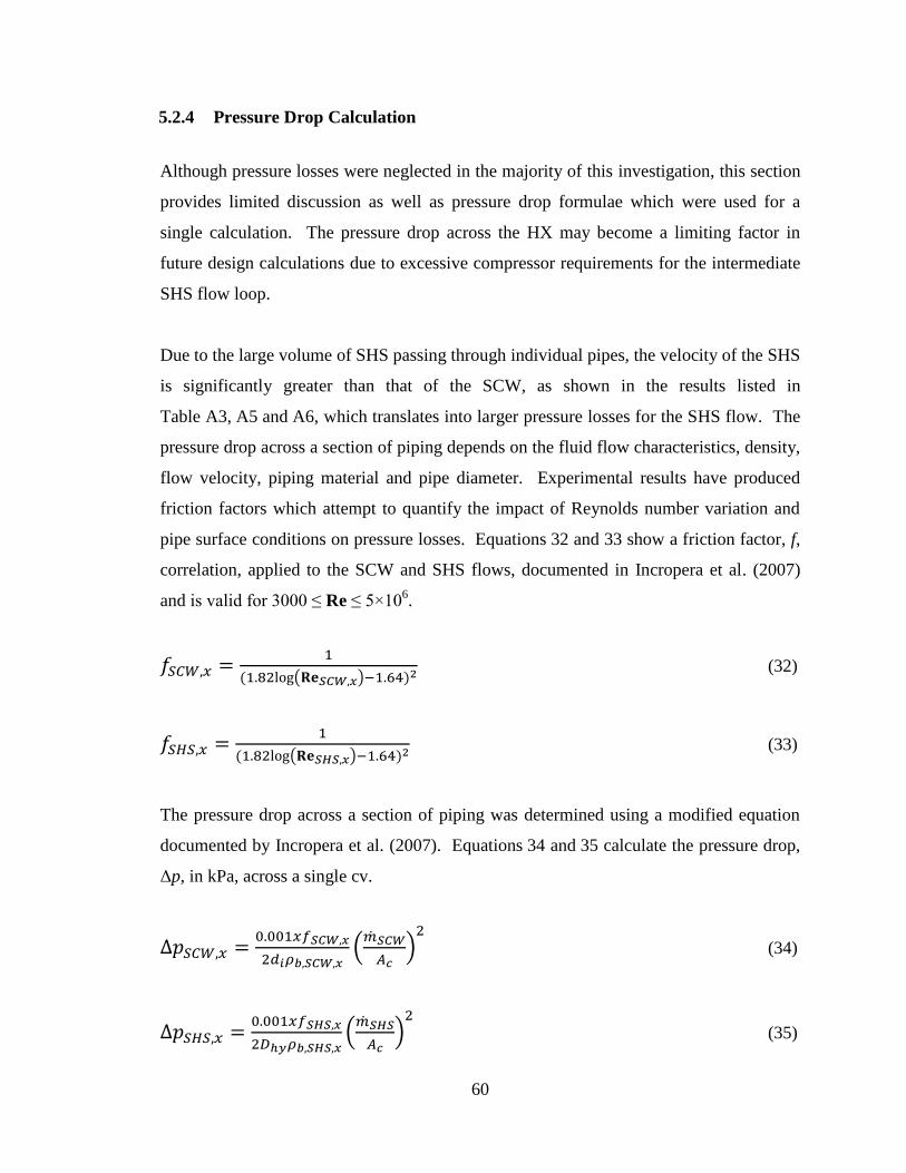
Figure 22. HX A Pipe Burst Pressure and Tensile Strength for SS–304 Pipes, Code
11222, 5–cm Interval. ....................................................................................................... 66
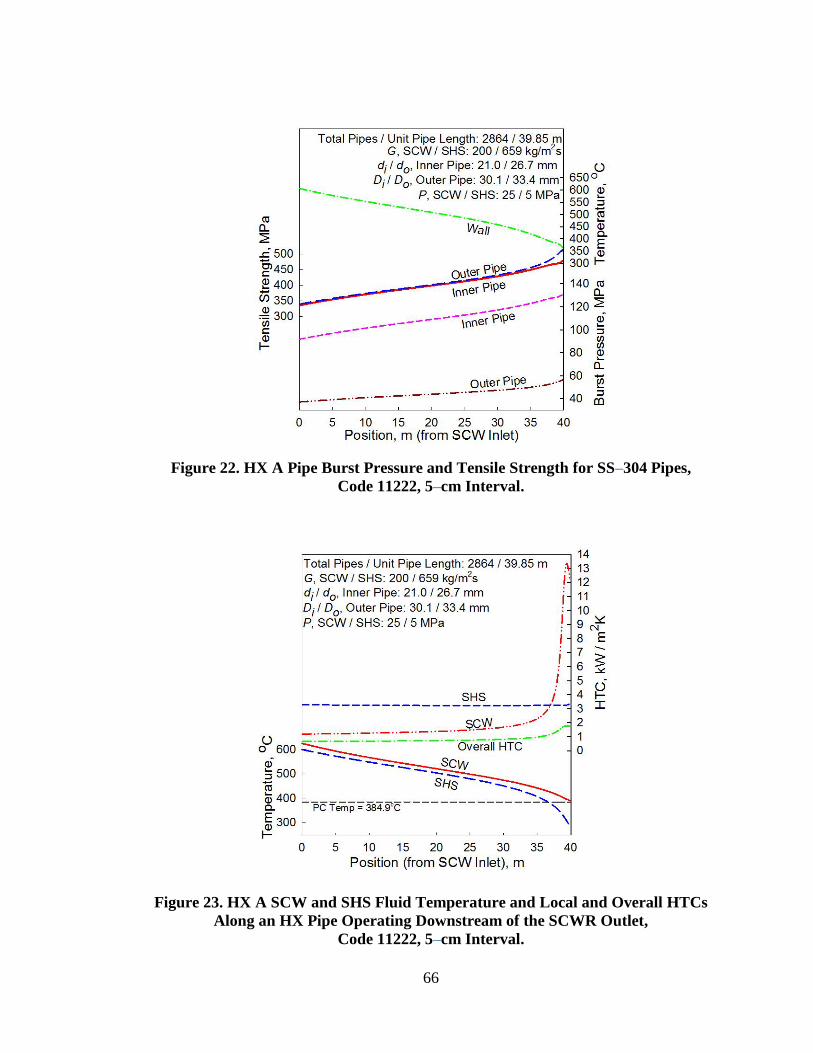
Figure 23. HX A SCW and SHS Fluid Temperature and Local and Overall HTCs Along
an HX Pipe Operating Downstream of the SCWR Outlet, Code 11222, 5–cm Interval. 66
Figure 24. HX A SCW and SHS Fluid Temperature and Thermal Resistances Along an
HX Pipe Operating Downstream of the SCWR Outlet, Code 11222, 5–cm Interval. ..... 67
Figure 25. HX A SCW Thermophysical Properties Along an HX Pipe Operating
Downstream of the SCWR Outlet Supporting the Mokry et al. Correlation, Code 11222,
5–cm Interval. ................................................................................................................... 67
Figure 26. HX A SCW Thermophysical Properties Along an HX Pipe Operating
Downstream of the SCWR Outlet Used in the Mokry et al. Correlation, Code 11222, 5–
cm Interval. ....................................................................................................................... 68
Figure 27. HX A SHS Thermophysical Properties Along an HX Pipe Operating
Downstream of the SCWR Outlet Used in the Mokry et al. Correlation, Code 11222, 5–
cm Interval. ....................................................................................................................... 68
Figure 28. HX A SHS Thermophysical Properties Along an HX Pipe Operating
Downstream of the SCWR Outlet Used in the Mokry et al. Correlation, Code 11222, 5–
cm Interval. ....................................................................................................................... 69
Figure 29. HX A SCW and SHS Fluid Temperature and Local and Overall HTCs Along
an HX Pipe, Code 13122, 10–cm Interval. ....................................................................... 71
Figure 30. HX A SCW and SHS Fluid Temperature and Local and Overall HTCs Along
an HX Pipe for Test Code 13132, 10–cm Interval............................................................ 71
Figure 31. HX A SCW and SHS Fluid Temperature and Local and Overall HTCs Along
an HX Pipe for Test Code 13232, 10‒cm Intervals. ......................................................... 72
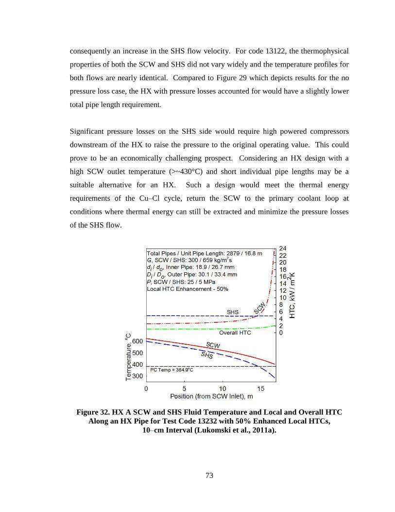
Figure 32. HX A SCW and SHS Fluid Temperature and Local and Overall HTC Along
an HX Pipe for Test Code 13232 with 50% Enhanced Local HTCs, 10–cm Interval
(Lukomski et al., 2011a). .................................................................................................. 73
Figure 33. HX A Impact of Theoretical Heat Transfer Enhancement of Local HTCs
(25%, 50% and 75%) on Overall HTC and HX Piping Requirements, 10–cm Intervals.
(Lukomski et al., 2011a). .................................................................................................. 74
Page 11
xi
Figure 34. HX A SCW and SHS Fluid Temperature and Pressure Loss Profiles Along an
HX Pipe for Code 13122, 5–cm Interval. ......................................................................... 74
Figure 35. Example of Poor HX A Test Code 11111 Where Operating Fluid
Temperature Difference Approaches Zero. ...................................................................... 75
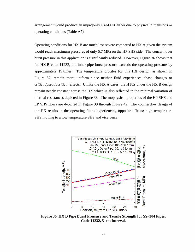
Figure 36. HX B Pipe Burst Pressure and Tensile Strength for SS–304 Pipes, Code
11232, 5–cm Interval. ....................................................................................................... 77
Figure 37. HX B HP SHS and LP SHS Fluid Temperature and Local and Overall HTCs
Along an HX Pipe Operating Downstream of the SCWR Outlet, Code 11232, 5–cm
Interval. ............................................................................................................................. 78
Figure 38. HX B HP SHS and LP SHS Fluid Temperature and Thermal Resistances
Along an HX Pipe Operating Downstream of the SCWR Outlet, Code 11232, 5–cm
Interval. ............................................................................................................................. 78
Figure 39. HX B HP SHS Thermophysical Properties Along an HX Pipe Operating
Downstream of the SCWR Outlet Supporting the Mokry et al. Correlation, Code 11232,
5–cm Interval. ................................................................................................................... 79
Figure 40. HX B HP SHS Thermophysical Properties Along an HX Pipe Operating
Downstream of the SCWR Outlet Used in the Mokry et al. Correlation, Code 11232, 5–
cm Interval. ....................................................................................................................... 79
Figure 41. HX B LP SHS Thermophysical Properties Along an HX Pipe Operating
Downstream of the SCWR Outlet Supporting the Mokry et al. Correlation, Code 11232,
5–cm Interval. ................................................................................................................... 80
Figure 42. HX B LP SHS Thermophysical Properties Along an HX Pipe Operating
Downstream of the SCWR Outlet Used in the Mokry et al. Correlation, Code 11232, 5–
cm Interval. ....................................................................................................................... 80
Page 12
xii
LIST OF TABLES
Table 1. Reactions Involved in the 4‒Step and 5‒Step Cu‒Cl Cycles (Naterer et al.,
2010). .................................................................................................................................. 7
Table 2. World Operating Nuclear Reactor Types (as of April 2011) (PRIS, 2011). ...... 13
Table 3. Overall Average and RMS Error for Heat Transfer Correlations in the
Subcritical Region (Zahlan et al., 2010). .......................................................................... 25
Table 4. Overall Weighted Average and RMS Error for Heat Transfer Correlations in the
Three Supercritical Sub-regions (Zahlan et al., 2010). ..................................................... 25
Table 5. Major Parameters of PT SCW CANDU (Mokry et al., 2011). ........................... 26
Table 6. Select Physical Properties and Composition of Materials Considered for
Intermediate HX (Matweb, 2011; Special Metals, 2011). ................................................ 38
Table 7. Pipe Dimensions in SCW Steam Generator Applications (Ornatskiy et al.,
1980). ................................................................................................................................ 41
Table 8. Operating Fluid Parameters for HX A (SCW/SHS). .......................................... 45
Table 9. Operating Fluid Parameters for HX B (HP SHS/LP SHS). ................................ 45
Table 10. Variation of SS‒304 Tensile Strength with Temperature ................................. 48
Table 11. Inner Pipe Dimensions with Wall Thickness to Outer Diameter Ratio. ........... 50
Table 12. Inner and Outer Pipe Dimension Combinations – ANSI Standards. ................ 50
Table 13. HX A Test Codes Developed for MATLAB Script. ........................................ 57
Table 14. HX B Test Codes Developed for MATLAB Script. ......................................... 57
Table 15. HX A and HX B Test Codes Analyzed in Chapter 6/Appendix B ................... 57
Table 16. HX A Design and Operating Parameter Variation for Code 11222 (5 MPa SHS
Pressure) and Code 21222 (4 MPa SHS Pressure). .......................................................... 70
Table 17. Comparison of HX B MATLAB Iterative Calculations and LMTD Method
Calculations for Code 11232. ........................................................................................... 81
Table A1. (As shown in Chapter 5) HX A Test Combinations Developed for MATLAB
Script. ............................................................................................................................... A1
Table A2. (As shown in Chapter 5) HX B Test Combinations Developed for MATLAB
Script. ............................................................................................................................... A1
Page 13
xiii
Table A3. HX A (SCW/SHS) MATLAB Results for Test Combinations Using 5 MPa
SHS Operating Fluid, 5–cm Intervals. ............................................................................. A2
Table A4. HX A (SCW/SHS) Unsuccessful MATLAB Results for Test Codes Using 5
MPa SHS Operating Fluid, 5–cm Intervals. .................................................................... A5
Table A5. HX A (SCW/SHS) MATLAB Results for Test Combinations Using 4 MPa
SHS Operating Fluid, 5–cm Intervals. ............................................................................. A6
Table A6. HX B (HP/LP SHS) MATLAB Results for Test Combinations Using 5 MPa
LP SHS Operating Fluid, 5‒cm Intervals. ....................................................................... A8
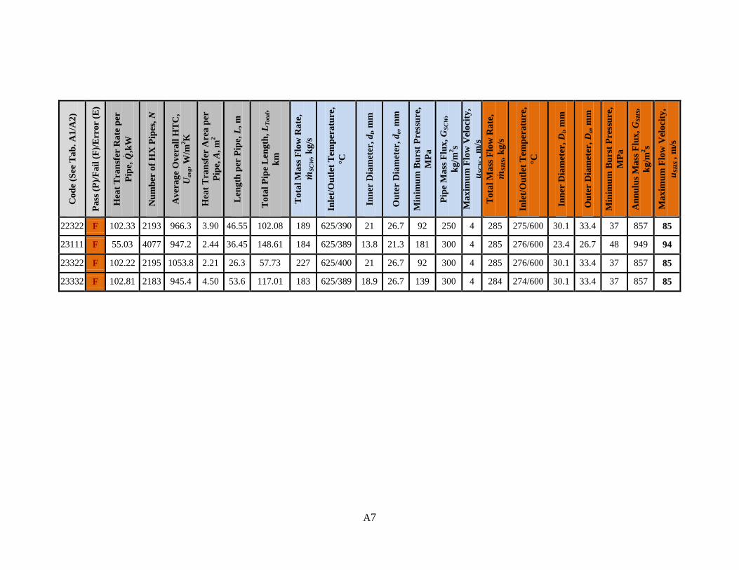
Table A7. HX B (HP/LP SHS) Unsuccessful MATLAB Results for Test Combinations
Using 5 MPa LP SHS Operating Fluid, 5–cm Intervals. ................................................. A9
Table B1. HX A (SCW/SHS) Code 11222 Comparison of CV SCW Outlet Temperatures
at Several HX Positions from MATLAB and Microsoft Excel. .................................... A10
Table B2. HX A (SCW/SHS) Code 11222 Comparison of SHS Inlet Temperatures at
Several HX Positions from MATLAB and Microsoft Excel. ........................................ A11
Table B3. HX A (SCW/SHS) Code 11222 Comparison of Wall Temperatures at Several
HX Positions from MATLAB and Microsoft Excel. ..................................................... A12
Table B4. HX B (HP/LP SHS) Code 12111 Comparison of HP SHS Outlet Temperatures
at Several HX Positions from MATLAB and Microsoft Excel. .................................... A13
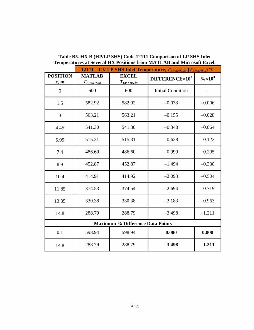
Table B5. HX B (HP/LP SHS) Code 12111 Comparison of LP SHS Inlet Temperatures at
Several HX Positions from MATLAB and Microsoft Excel. ........................................ A14
Table B6. HX B (HP/LP SHS) Code 12111 Comparison of Wall Temperatures at Several
HX Positions from MATLAB and Microsoft Excel. ..................................................... A15
Page 14
xiv
NOMENCLATURE
A: Area, m2
: Specific Heat, J/kg K
cp,avg: Average Specific Heat, J/kg K;
D, d: Diameter, m
f: Friction factor
G: Mass Flux, kg/m2s;
H: Specific Enthalpy, J/kg
h: Heat Transfer Coefficient, W/m2K
k: Thermal Conductivity, W/m K
L: Length, m
: Mass Flow Rate, kg/s
N: Number of Pipes in an HX
P: Pressure, Pa
p: Perimeter, m
Q: Thermal Energy, J
Heat Transfer Rate, W
Heat Flux, W/m2;
R: Thermal Resistance, K m2/W
S: Tensile Strength, MPa
T: Temperature, °C, K
U: Overall Heat Transfer Coefficient, W/m2K
u: Velocity, m/s;
Page 15
xv
V: Electrical Energy, J
x: Axial Position, m
Greek symbols
Δ: Difference
ρ: Density, kg/m3
μ: Viscosity, Pa·s
: Wall Thickness, m
Dimensionless Numbers
Nu: Nusselt Number
Inner Pipe;
Annulus Gap
: Prandtl Number
: Average Prandtl Number
: Reynolds Number
Inner Pipe;
Annulus Gap
Subscripts
avg: average
b: bulk
c: cross section
cr: critical
el: electrical
hy: hydraulic
i: inner
inc: increment
lm: log mean
o: outer
pc: pseudocritical
Page 16
xvi
s: surface
sat: saturation
x: increment position
w: wall
wet: wetted
Acronyms
ACR Advanced CANDU Reactor
AECL Atomic Energy of Canada Limited
ANL Argonne National Laboratory
BWR Boiling Water Reactor
CANDU CANada Deuterium Uranium
Cu‒Cl Copper Chlorine
cv Control Volume
FHR Fluoride-cooled High temperature Reactor
GE General Electric
GFR Gas-cooled Fast Reactor
GIF Generation IV International Forum
HP High Pressure
HTC Heat Transfer Coefficient
HTE High-Temperature Electrolysis
HX Heat eXchanger
IP Intermediate Pressure
JAERI Japan Atomic Energy Research Institute
LFR Lead-cooled Fast Reactor
LMTD Log Mean Temperature Difference
Page 17
xvii
LP Low Pressure
MATLAB MATrix LABoratory
MSR Molten Salt Reactor
MSFR Molten Salt Fast Reactor
MOX Mixed OXide
NHI Nuclear Hydrogen Initiative
NIST National Institute of Standards and Technology
NPP Nuclear Power Plant
PHWR Pressurized Heavy Water Reactor
PT Pressure Tube
PV Pressure Vessel
PWR Pressurized Water Reactor
REFPROP REference Fluid thermodynamic and transport PROPerties
RMS Root Mean Square
SCW SuperCritical Water
SCWR SuperCritical Water Reactor
SFR Sodium-cooled Fast Reactor
SHS SuperHeated Steam
SI Sulphur Iodine
SMR Steam Methane Reforming
STP Standard Temperature - Pressure
UO University of Ottawa
UOIT University of Ontario Institute of Technology
VHTR Very High-Temperature Reactor
Page 18
xviii
GLOSSARY
Definitions of select terms related to supercritical and near-critical fluids and are
provided to support discussion on SuperCritical Water-cooled nuclear Reactors (Pioro
and Duffey, 2007). Figure i1 may also assist to provide a better understanding of the
terms that have been defined.
Compressed fluid is a fluid at a pressure above the critical pressure but at a temperature
below the critical temperature.
Critical point (also called a critical state) is the point where the distinction between the
liquid and gas (or vapour) phases disappears, i.e. both phases have the same temperature,
pressure and volume. The critical point is characterized by the phase state parameters
Tcr, Pcr and Vcr, which have unique values for each pure substance.
Deteriorated heat transfer is characterized with lower values of the wall heat transfer
coefficient compared to those at the normal heat transfer; and hence has higher values of
wall temperature within some part of a test section or within the entire test section.
Improved heat transfer is characterized with higher values of the wall heat transfer
coefficient compared to those at the normal heat transfer; and hence lower values of wall
temperature within some part of a test section or within the entire test section.
Near-critical point is a narrow region around the critical point where all the
thermophysical properties of a pure fluid exhibit rapid variations.
Normal heat transfer can be characterized in general with wall heat transfer coefficients
similar to those of subcritical convective heat transfer far from the critical or
pseudocritical regions, when calculated according to the conventional single-phase
Dittus-Boelter type correlations.
Pseudocritical point (characterized with ppc and tpc) is a point at a pressure above the
critical pressure and at a temperature (tpc> tcr) corresponding to the maximum value of
the specific heat for this particular pressure.
Page 19
xix
Pseudocritical line is a line consisting of pseudocritical points.
Pseudocritical region is the region of temperatures, typically listed as ±25°C from the
pseudocritical temperature for a given pressure where thermophysical properties of a
pure fluid exhibit rapid changes - this analogous to the near-critical point.
Supercritical fluid is a fluid at pressures and temperature that are higher than the critical
pressure and critical temperature.
Supercritical steam is actually supercritical water because at supercritical pressures
there is no difference between phases. However, this term is widely and incorrectly used
in the literature in relation to supercritical steam generators and turbines.
Superheated steam is steam at a pressure below the critical pressure but at temperatures
above the critical temperature.
Axial Location, m
0.0 0.5 1.0 1.5 2.0 2.5 3.0 3.5 4.0
Te
mp
era
ture
, oC
300
350
400
450
600
550
500
Bulk Fluid Enthalpy, kJ/kg
1400 1600 1800 2000 2200 2400 2600 2800
HT
C,
kW
/m2K
2
4
8
12
1620
28
36
Heated length
Bulk fluid temperature
tin
tout
Inside wall temperature
Heat transfer coefficient
pin=24.0 MPa
G=503 kg/m2s
Q=54 kW
qave
= 432 kW/m2
C381.1t o
pc
Hpc
Dittus - Boelter correlation
DHT Improved HT
Normal HTNormal HT
(a) (b)
Figure i1. (a) Pressure-Temperature Diagram for Water; (b) Temperature and Heat
Transfer Coefficient Profiles Along the Heated Length of a Vertical Circular Tube:
Water, D=10 mm and L=4 m. (Pioro et al., 2011).
Page 20
1
INTRODUCTION
Hydrogen, as an energy carrier, could develop to have a significant role in the future
energy supply of industrialized nations. Although carbon based fuel sources such as oil
and gas will continue to dominate the energy landscape in the near future it is unlikely
that they will be capable of fulfilling the entire energy requirements of the global
economy as more nations industrialize while sources continue to be depleted. For other
traditional energy sources such as coal, more stringent environmental restrictions on
carbon emissions may lead to reduced consumption levels. Such projections warrant a
need for an alternative energy source to offset a fraction of the energy consumed via oil,
gas and coal sources.
Hydrogen, produced through non-carbon based methods may increase penetration with
time into the automotive, food and agricultural industry as a shift in energy sources is
realized. Thermochemical hydrogen production is one of several methods being
researched that could provide a large supply of hydrogen through centralized generation
facilities. Using water and external thermal energy (for hybrid cycles - thermal and
electrical energy) as inputs, a thermochemical cycle decomposes water into hydrogen and
oxygen while continuously recycling a number of intermediate compounds. Various
thermal energy sources may be integrated with thermochemical cycles to supply reaction
heat, including nuclear and solar power plant facilities.
The intent of this research was to conduct an evaluation of the feasibility for linking a
Generation IV nuclear reactor, the SuperCritical Water-cooled nuclear Reactor (SCWR)
concept, and a hydrogen production facility operating on the Copper Chlorine (Cu‒Cl)
thermochemical cycle through a Heat eXchanger (HX) transferring thermal energy
between the facilities. The research scope involved performing a literature survey of
recent developments in Cu‒Cl cycle research, Generation IV nuclear reactor designs,
specifically the SCWR, and applicable heat transfer correlations to be considered
followed by analysis to determine suitable design and operating conditions for an HX
linking the two facilities. The original work involved thermalhydraulic calculations
Page 21
2
based on an iterative energy balance procedure for HXs with various design parameters
and operating conditions. Certain inputs were based on existing design information for
the SCWR concept and known operating conditions of the 4-step Cu‒Cl cycle. In
addition, operating experience from the Russian steam generator industry was
incorporated to define acceptable HX piping dimensions. Theoretical enhancement of
local Heat Transfer Coefficients (HTC) was considered through the use of helically
corrugated pipes to reduce the physical size of the HX.
Chapter 1 provides a background and discussion on several hydrogen production methods
that are used today such as Steam Methane Reforming (SMR) and gasification
technology. Emerging processes such as High-Temperature Electrolysis (HTE) and
thermochemical cycles are also described with specific focus on the Cu–Cl cycle. The
reaction steps within the cycle are briefly discussed and the external thermal energy
requirements are outlined. Chapter 2 provides insight into the six Generation IV reactor
concepts currently under development. Chapter 3 discusses SuperCritical Water (SCW)
and relevant heat transfer correlations considered in this analysis. Chapter 4 describes the
Nuclear Power Plant (NPP) cycle layouts considered suitable for linking the facilities:
i) no-reheat cycle; and ii) single reheat cycle. It also contains discussion on HX design
options and use of the Log Mean Temperature Difference (LMTD) method for select HX
analysis. The methodology employed to conduct thermalhydraulic calculations is
outlined in Chapter 5. Chapter 6 is dedicated to results and the discussion of research
findings. Conclusions are presented in Chapter 7 and recommendations for future work
are listed in Chapter 8. Appendix A contains a summary of all results obtained from the
thermalhydraulic analyses. Tables documenting the verification of results are contained
in Appendix B. A summary of the calculations involved in this work are contained in
Appendix C. The MATLAB script, used as the primary calculation tool is documented in
Appendix D. Finally, publications by the author and a list of presentations at conferences
are presented in Appendices E and F, respectively.
Page 22
3
CHAPTER 1 – HYDROGEN PRODUCTION
Hydrogen is the most abundant element in the universe. However, it is not readily
available in its molecular form and must be extracted from water or hydrocarbons for
commercial and industrial applications. Currently, the most popular and least expensive
method of hydrogen production is through steam reforming of fossil fuels (i.e. Steam
Methane Reforming (SMR)) accounting for approximately 50% of world hydrogen
production (Press et al., 2009). Jones and Thomas (2008) quote the fraction as high as
90% of the world’s supply. If hydrogen is to become a sustainable energy carrier source
in the future global economy, reliance on fossil fuels for its production must be
significantly reduced.
Gasification and SMR are the most common fossil fuel-based hydrogen production
methods. Gasification involves the net-exothermic reaction of carbon-based materials
such as coal, methane or other petrochemical by-products with steam and oxygen under
reducing conditions. Required reaction chamber operating temperatures and pressures of
gasifiers are on the order of 1,250 to 1,575°C and 2 MPa (Jones and Thomas, 2008). The
resulting products, a mix of carbon monoxide and hydrogen gases, generically known as
synthetic (syn) gas, are separated for various applications. The H2/CO ratio of the
product varies depending on the gasifier type, the oxygen concentration, reactant feed
rate, and the carbon feedstock composition; for example, natural gas typically has a
H2/CO ratio of 1.75 whereas coal has a ratio of 0.80 (Jones and Thomas, 2008). The CO
gas component of syngas can be further reacted with steam at high temperatures under
the water gas shift reaction to generate more hydrogen gas and carbon dioxide.
In SMR, fossil fuels such as methane gas are reacted with steam over a nickel-based
catalyst at high temperatures producing syngas. The reaction involving methane is
endothermic requiring 252 kJ per mole of methane at standard temperature-pressure
(STP) conditions. Addition of oxygen into this reaction creates an autothermal reformer,
where the exothermic methane/oxygen reaction, known as a partial oxidation reaction,
assists in providing heat for the primary reaction (Rand and Dell, 2008).
Page 23
4
Nuclear-based hydrogen production may be achieved through water electrolysis or steam
electrolysis, which requires a combination of high temperatures and electrical energy
input. The latter process involves directing steam from an NPP to a solid-oxide
electrolyte. Efficiencies for HTE can reach up to 50 ‒ 60%, as documented by Jones and
Thomas (2008), due to the lower electrical overpotentials required, improved gas
diffusivity and the thermal energy by-product (Ryland et al., 2006). Ryland et al. (2006)
investigated the linkage of the Advanced CANDU (CANada Deuterium Uranium)
Reactor (ACR-1000) design concept developed by Atomic Energy of Canada Limited
(AECL) to an HTE facility, which predicted efficiencies of approximately 35%.
The Sulphur Iodine (SI) thermochemical cycle is a 3-Step reaction process, which has
been widely investigated in several countries under laboratory-scale test loops. A
research facility operated by the Japan Atomic Energy Research Institute (JAERI) has
produced a hydrogen output up to 30 L/h (Jones and Thomas, 2008). The process
involves the decomposition of sulfuric acid at temperatures above 800°C, processing of
intermediate liquid and gas materials and further decomposition of hydrogen iodide to
produce hydrogen. Efficiencies as high as 50% have been predicted for this cycle (Jones
and Thomas, 2008). Due to the extreme reaction temperatures of the SI cycle, only
certain technologies can meet this requirement, including the modular helium reactor
which is characterized by reactor outlet temperatures up to 850°C (Richards et al., 2006).
Hydrogen production via thermochemical cycles has become a leading alternative to
fossil-based production methods. Thermochemical cycles are desirable over traditional
electrolysis methods given the higher production efficiency. Over 200 thermochemical
cycles have been identified in literature, however, the vast majority have not progressed
beyond theoretical calculations due to various limitations including high temperature
requirements and/or low efficiencies (Naterer et al., 2008). Efforts by Argonne National
Laboratory (ANL) in the US and by researchers in other universities in Europe, Japan,
South Africa and the US are undergoing through the Nuclear Hydrogen Initiative (NHI)
to evaluate thermochemical cycles identifying those most suitable for development. The
Page 24
5
following factors have been considered: chemical viability (no significant competing
reactions/high yields), engineering feasibility (simulated operation) and efficiency. The
cycles under evaluation were: cerium-chlorine (Ce‒Cl), copper chlorine (Cu‒Cl), iron-
chlorine (Fe‒Cl), vanadium-chlorine (V‒Cl), copper sulphate (Cu‒SO4), magnesium-
iodine (Mg‒I), hybrid chlorine and a metal alloy cycle potassium-bismuth (K‒Bi) (Lewis
and Masin, 2009). The majority of these cycles are characterized by low efficiencies,
undesirable by-products, poor chemical kinetics or high-temperature requirements. From
eight contending cycles, the Cu‒Cl cycle was selected as the most promising cycle
warranting continued research and development (Lewis and Masin, 2009). Research into
thermochemical cycles such as the Cu‒Cl cycle will advance the objective of the NHI to
develop a cost effective nuclear based hydrogen production facility by 2019 (Lewis and
Masin, 2009).
Teams at several institutions including the University of Ontario Institute of Technology
(UOIT), AECL and ANL are currently advancing the research efforts on the 4-Step
hybrid Cu‒Cl cycle. Research involves scaling up and integrating a proof of principle
experimental set-up to engineering scale assemblies capable of producing up to 3 kg of
hydrogen per day (Wang et al., 2009).
1.1 COPPER-CHLORINE CYCLE
The Cu‒Cl cycle has been selected as the most suitable thermochemical cycle to be
interlinked with an SCWR (Naidin et al., 2009c). Several favourable characteristics of
the Cu‒Cl cycle make it an attractive process for hydrogen production. These include a
relatively low maximum temperature requirement (~530°C), favourable reaction kinetics
for the oxygen and hydrogen-production steps and the availability to utilize waste heat to
supply endothermic processes (Naterer et al., 2009). Various forms of the Cu‒Cl cycle
exist, including a 2-Step process proposed by Dokiya and Kotera (1976), 3-Step, 4-Step
and 5-Step processes documented by Naterer et al. (2008) and Wang et al. (2009).
Page 25
6
The 5-Step Cu‒Cl cycle is comprised of an exothermic hydrogen production step, three
endothermic processes and an electrolysis step as shown Figure 1. The 4-Step variation
combines the hydrogen production and electrolysis steps of the 5-Step process into a
single electrochemical reaction which is shown in Figure 2. This step is analogous to that
proposed by Dokiya and Kotera (1976). The associated reactions for both cycles are
shown in Table 1 and described below in more detail.
In Step 1 of the 5-Step cycle, solid copper particles react with high-temperature hydrogen
chloride gas resulting in the production of hydrogen gas and liquid cuprous chloride.
Although the reaction is exothermic, reactants must initially be heated to the threshold
temperature of approximately 475°C. Step 1 provides one of the advantages of the
5-Step cycle which is the by-product of high-temperature thermal energy as up to
139.8 MJ can be recycled for every kilogram of hydrogen produced stemming from
cooling of products and recovery of reaction heat. A major disadvantage of the 5-Step
cycle is the production and handling of solid copper compounds, which requires an
additional drying process thus increasing heat demand and complexity of the cycle.
The second reaction in the 5-Step cycle would involve an electrochemical reaction using
a feed of solid CuCl undergoing oxidation at ambient temperature to produce an aqueous
solution of CuCl2 and solid copper particles which would be routed to the hydrogen
production reactor (Step 1). Chemical kinetics would be dependent on the operating
temperature and pressure of the reactor and the composition of the reactants (Naterer et
al., 2009b). Naterer et al. (2008) outlined the electrical energy requirements to be
approximately 31 MJ per kilogram of hydrogen produced. Giving rise to the 4-Step
cycle, the combination of the first two reactions into a new electrolysis reaction occurring
at temperatures of approximately up to 100°C would produce hydrogen and copper
chloride electrolytically. Such a reaction would avoid the production of solid copper and
the required drying facilities simplifying the processes of the cycle. Research focus in
literature has gradually shifted towards the 4-Step cycle, due in part to the less complex
design requirements associated with the cycle.
Page 26
7
Table 1. Reactions Involved in the 4-Step and 5-Step Cu‒Cl Cycles
(Naterer et al., 2010).
Step Reaction
Temp.
Range
(°C)
Feed/Output
1* 2CuCl (aq) + 2HCl (aq) →
H2 (g) + 2CuCl2 (aq)
Electrolysis
(Hydrogen
Production)
~100 Feed
Aqueous CuCl and HCl
+ V + Q Electrolytic Cu
+ dry HCl + Q
Output H2 + CuCl2 (aq)
2 CuCl2 (aq) → CuCl2 (s) Drying <100
Feed Slurry containing HCl
and CuCl2 + Q
Output Granular CuCl2 +
H2O/HCl vapours
3 2CuCl2 (s) + H2O (g) →
CuO*CuCl2 (s) + 2HCl (g) Hydrolysis 375‒400
Feed Powder/granular CuCl2
+ H2O (g) + Q
Output Powder/granular
CuO*CuCl2 + 2HCl (g)
4 CuO*CuCl2 (s) →
2CuCl (l) + 1/2O2 (g)
Oxygen
Production 530‒550
Feed Powder/granular
CuO*CuCl2 (s) + Q
Output Molten CuCl salt +
oxygen
Q, thermal energy; V, electrical energy
* 5-Step Cycle Reaction 1: a) 2Cu (s) + 2HCl (g) → 2CuCl (l) + H2 (g) at 450°C
b) 2CuCl (aq) = Cu (s) + CuCl2 (aq) in HCl solution at 30-80°C
In Step 3 of the cycle, solid cupric chloride is obtained from the drying of a slurry or
solution of HCl/CuCl2 in preparation for the hydrolysis reaction. Naterer et al. (2008)
determined that drying a solution rather than a slurry precipitate would be the most heat-
intensive step in the cycle increasing the overall heat requirement of the facility by a
factor of 2.5. For the 5-Step cycle, with a slurry drying process, the overall thermal
energy requirement of the 5-Step cycle (endothermic reactions, heating of reactants and
drying processes) would be approximately 277 MJ per kilogram of hydrogen produced
while the heat released (heat of reaction, cooling of reaction products and solidification of
materials) would be approximately 116 MJ per kilogram of hydrogen (Naterer et al.,
2008). Low grade waste heat could be utilized for this reaction given the temperature
requirements are much lower compared to the other endothermic reactions in the cycle.
Page 27
8
For the purposes of this research, the thermal energy requirements of this step were
included into the overall energy demand of the cycle.
The hydrolysis reaction of the Cu‒Cl cycle involves CuCl2 and SuperHeated Steam
(SHS) undergoing an endothermic reaction at temperatures of approximately 375°C
(Naterer et al., 2009a). Solid particles of CuCl2 obtained from Step 3 are fed into a steam
stream to produce copper oxychloride (CuO*CuCl2) and hydrochloric gas. Copper
oxychloride is important in the downstream oxygen production reactor while cuprous
chloride is required in the hydrogen production step (5-Step cycle) and the
electrochemical reaction (4-Step cycle).
The final reaction in the Cu‒Cl cycle leads to the production of oxygen through the
decomposition of the copper oxychloride obtained in Step 4. This high-temperature
reaction occurs at approximately 530°C and produces oxygen gas and liquid cuprous
chloride which is fed to the electrolysis reaction after being converted to a solid.
Developing a heat exchange network to enable this reaction has been considered by
Naterer et al. (2008). One method, further discussed in Chapter 4, would use a
circulating loop of molten CuCl heated in a nuclear or solar power plant based HX and
delivered directly into the reaction vessel to provide reaction heat. Alternatively, a
molten salt would be heated through an HX by external heat sources and then pass
through a shell around the reaction vessel providing indirect heating of the reactants. In
this research, the SHS flowing between the NPP and hydrogen production facility can be
viewed as the molten salt equivalent supplying external thermal energy to the cycle.
Page 28
9
Input,
H2O(l)
Output,
H2(g)
Output,
O2(g)
H2O(g)
Heat
Recovery
H2
Production
Reactor
Step 1
~475°C
H2O(l)
CuCl2 +
H2O
CuCl(s)
CuCl(l)
Cu(aq)
HCl(g)
Cu2OCl2(s)
Heat
Heat
Heat
Heat
H2(g)
CuCl2(s)
Cu(s)
CuCl(l)
Drying
Step 3
<100°C
Hydrolysis
Step 4
~400°C
O2
Production
Step 5
~530°C
Electrolysis
Step 2
Ambient
Conditions
Heat
Recovery
Heat
Figure 1. Conceptual Cu–Cl Cycle Layout Based on a 5-Step Process
(adapted from Naterer et al., 2008; Lukomski et al., 2010b).
Page 29
10
It is desirable to maximize the amount of thermal energy recycled within the Cu‒Cl cycle
such that it may be transferred between reactions in the cycle and external heat source
requirements are reduced. A fraction of the heat produced within the cycle is considered
to be low grade, such as low-temperature water or solid powders from which thermal
energy may not be used effectively; such barriers may limit the full scale development of
Cu‒Cl cycle facilities (Wang et al., 2008). Wang et al. (2010a) assessed that
approximately 50% of the heat generated within the cycle is recoverable for useful
purposes. Wang et al. (2010b) further showed that the SI and Cu‒Cl cycles have similar
hydrogen production costs and if effective internal heat recycling is achieved they will
have an efficiency advantage over conventional electrolysis methods.
Measures to reduce external heat demand have been explored by Wang et al. (2009) in
the form of a proposed modified Cu‒Cl cycle requiring lower excess steam for the
hydrolysis reaction. An excess of steam is required to progress the hydrolysis reaction to
completion such that a high yield of product can be obtained and formation of impurities
such as CuCl and Cl2 can be minimized (Lewis et al., 2009). Wang et al. (2009) showed
that increasing the steam to CuCl2 ratio in the hydrolysis reaction does not significantly
reduce the heat required by the reaction.
The shift in focus toward a 4-Step Cu‒Cl process has eliminated a large source of
exothermic heat from the cycle normally generated in the thermochemical hydrogen
production step (Step 1 of the 5-Step cycle) shown in Table 1. Considering the
thermochemical reactions in the 4-Step cycle (Step 3, 4 and 5), the net heat input required
by the cycle is 247 kJ/g of hydrogen with a recoverable fraction of 46 kJ/g (Wang et al.,
2010b). Accounting for the 50% of recyclable thermal energy, the net external thermal
energy, Q, required by the 4-Step cycle is 224 kJ for each gram of hydrogen produced.
This value is used as an input into the thermalhydraulic calculations performed for the
HXs considered in this analysis. It is important to note that heat losses have not be
considered in this work, however, the requirements of step 2 (drying stage) have been
accounted for even though they are considered low temperature steps and could be met
by sources of waste heat.
Page 30
11
Figure 2. Conceptual Layout for the 4-Step Cu‒Cl Cycle
(adapted from Naterer et al., 2010).
Page 31
12
CHAPTER 2 – GENERATION IV NUCLEAR REACTOR DESIGNS
The energy needs of the future will be met by a diverse mix of technologies based on
traditional fossil fuel sources, nuclear fuels and emerging renewable sources such as wind
and solar power. The role played by nuclear power will grow worldwide as nations
embark on new nuclear programs while others re-consider nuclear power as a viable, safe
and efficient alternative for electrical generation. Concurrent to a renewed worldwide
interest in the industry, the development of the next generation of nuclear reactor is
underway.
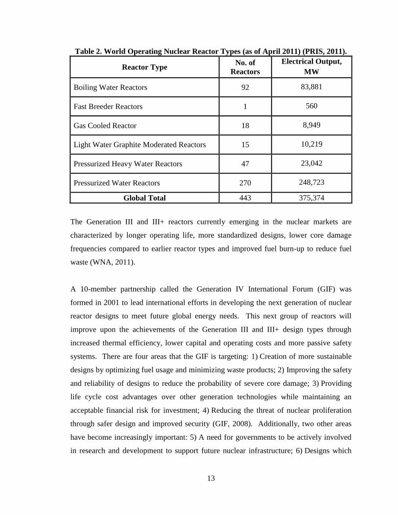
The majority of the 443 nuclear reactors currently operating around the world are part of
the second generation of reactor design and include the Pressurized Water Reactor
(PWR), Boiling Water Reactor (BWR) and Pressurized Heavy Water Reactor (PHWR) as
shown in Table 2. Designed predominantly in the 1960s and 1970s with 40-year planned
life cycles, many of the early constructions will approach their end of life in the next two
decades. Figure 3 shows a distribution of world-wide operating reactor status with a
large portion, over 80% above 20 years old. In the absence of renewed growth, the
global nuclear industry will experience a significant decline in the next two decades.
Figure 3. World-wide Status of Currently Operating Nuclear Reactors (PRIS, 2011).
Page 32
13
Table 2. World Operating Nuclear Reactor Types (as of April 2011) (PRIS, 2011).
Reactor Type No. of
Reactors
Electrical Output,
MW
Boiling Water Reactors 92 83,881
Fast Breeder Reactors 1 560
Gas Cooled Reactor 18 8,949
Light Water Graphite Moderated Reactors 15 10,219
Pressurized Heavy Water Reactors 47 23,042
Pressurized Water Reactors 270 248,723
Global Total 443 375,374
The Generation III and III+ reactors currently emerging in the nuclear markets are
characterized by longer operating life, more standardized designs, lower core damage
frequencies compared to earlier reactor types and improved fuel burn-up to reduce fuel
waste (WNA, 2011).
A 10-member partnership called the Generation IV International Forum (GIF) was
formed in 2001 to lead international efforts in developing the next generation of nuclear
reactor designs to meet future global energy needs. This next group of reactors will
improve upon the achievements of the Generation III and III+ design types through
increased thermal efficiency, lower capital and operating costs and more passive safety
systems. There are four areas that the GIF is targeting: 1) Creation of more sustainable
designs by optimizing fuel usage and minimizing waste products; 2) Improving the safety
and reliability of designs to reduce the probability of severe core damage; 3) Providing
life cycle cost advantages over other generation technologies while maintaining an
acceptable financial risk for investment; 4) Reducing the threat of nuclear proliferation
through safer design and improved security (GIF, 2008). Additionally, two other areas
have become increasingly important: 5) A need for governments to be actively involved
in research and development to support future nuclear infrastructure; 6) Designs which
Page 33
14
will enable cogeneration producing energy sources other than electricity (GIF, 2009).
Members are focusing on six reactor design concepts that are intended to form the
foundation of the future nuclear industry. Commercial integration of Generation IV
systems is expected to occur by 2030, as shown in Figure 4.
Figure 4. Evolution of Nuclear Reactor Designs (Generation IV Forum, 2008).
A general background of the six design concepts based on details from the GIF is
presented with a more detailed review of the SCWR and associated potential NPP design
layouts which could be selected for cogeneration applications.
The Sodium-cooled Fast Reactor (SFR) design concept would operate in the fast neutron
spectrum using liquid sodium as the primary coolant with reactor outlet conditions
of 550°C. A closed fuel cycle would be employed with either metal alloy or Mixed
OXide (MOX) fuel allowing for high level waste recycling. In terms of development,
this design holds an advantage over other Generation IV designs as SFRs have already
been constructed in a number of European countries and Japan (Lineberry and
Allen, n.d). As a result, the deployment of SFR technology could occur as early as 2020.
Page 34
15
Due to the relatively low reactor outlet temperature, hydrogen cogeneration via
thermochemical cycles has not been considered for SFR technology.
As with the SFR, the Lead-cooled Fast Reactor (LFR) would operate in the fast neutron
spectrum with a closed nuclear fuel cycle. The low pressure LFR coolant would be either
lead or a lead-bismuth eutectic with a metal or nitride nuclear fuel. Increased operating
temperatures ranging between 550°C and 800°C could enable thermochemical hydrogen
production, however, the proposed SSTAR and ELSY designs would operate at the lower
end of this range. Long term development of the LFR could see the rise of materials with
reduced lead corrosion rates at higher temperatures allowing for the development of a
more advanced reactor design by 2035. Lower temperature designs are anticipated to
emerge around 2025.
The Molten Salt Reactor (MSR) would operate at pressures below 500 kPa with a coolant
mixture of uranium and plutonium fuel dissolved in a molten fluoride salt mixture. There
are various evolutions of the MSR design; however, current focus is on the fast-spectrum
MSR (MSFR) and Fluoride-cooled High temperature Reactor (FHR). Advantages of this
design include a low fuel inventory and continuous recycling of actinides. The operating
temperatures of such reactors could range between 700 ‒ 800°C which would be suitable
for thermochemical hydrogen production via the Cu‒Cl cycle.
Operating with helium coolant, the Gas-cooled Fast Reactor (GFR) concept would
operate in the fast neutron spectrum with outlet temperatures of 850°C achieving high
thermal efficiencies. The reactor would operate on a closed fuel cycle with nitride or
carbide based fuels embedded with uranium or plutonium. It would be capable of
supplying thermal energy for hydrogen production via the Cu‒Cl cycle or the SI cycle.
The technology used in the GFR is similar in nature to the Very-High Temperature
Reactor (VHTR) which would also be cooled by helium.
The VHTR would operate in the thermal neutron spectrum with the helium coolant
passing through a graphite moderated core at temperatures of up to 1,000°C. The fuel
Page 35
16
would be comprised of a uranium oxide pebble or prism. Due to the very high coolant
outlet temperature, this reactor design would be suitable in process heating applications,
specifically hydrogen production through the SI and Cu‒Cl cycles.
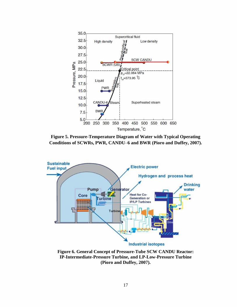
The SCWR is a design concept using SCW as a coolant with reactor inlet and outlet
temperatures of 350°C and 625°C, respectively. The reactor would operate above the
thermodynamic critical point of water (approx. 22.1 MPa, 374°C) where water exists in a
single phase state with characteristics of a low density liquid. Two reactor options would
be possible for such a reactor: a Pressure Vessel (PV) similar to conventional PWR or
BWR reactors or a Pressure Tube (PT) design as an evolution of the CANDU-type
PHWR. Due to the increased temperature and pressure of the coolant, such a reactor
would operate at efficiencies of approximately 50%, much higher than current nuclear
facilities which typically achieve efficiencies of 29 - 34%. The typical operating
conditions for several reactor design types are shown in Figure 5. An SCWR design
would also enable the direct use of the coolant for expansion in turbines for electricity
production, cogeneration of hydrogen via thermochemical cycles, production of industrial
isotopes and desalination applications. Figure 6 and 7 depict a PT type and PV type
concept, respectively, with the various economic benefits that would stem from such
systems.
Although there are two main SCWR design options under consideration there are several
potential NPP cycle layouts that can be integrated with the reactor and will be further
discussed in Chapter 4.
Page 36
17
Figure 5. Pressure-Temperature Diagram of Water with Typical Operating
Conditions of SCWRs, PWR, CANDU‒6 and BWR (Pioro and Duffey, 2007).
Figure 6. General Concept of Pressure-Tube SCW CANDU Reactor:
IP-Intermediate-Pressure Turbine, and LP-Low-Pressure Turbine
(Pioro and Duffey, 2007).
Page 37
18
Figure 7. Schematic of US Pressurized-vessel SCW Nuclear Reactor
(Pioro and Duffey, 2007).
Page 38
19
CHAPTER 3 – SUPERCRITICAL WATER AND HEAT
TRANSFER CORRELATIONS
Water is in a supercritical state when its pressure is above 22.064 MPa and its
temperature exceeds 374°C. This boundary state is termed the critical point. Above this
point, there is no visible phase distinction and the fluid is characteristic of a low density
liquid. Another phenomenon that occurs as water passes through the critical point is a
rapid variation in thermophysical properties (Pioro and Duffey, 2007). Most notably, the
specific heat of water exhibits a peak at the critical point.
Variations in properties are also exhibited at pressure and temperature combinations
above the critical point; however, they are not as significant and become less profound
with increasing pressure. These regions are termed pseudocritical and the pseudocritical
point is defined as the fluid state above the critical point (temperature and pressure)
having a maximum specific heat. The pseudocritical region ranges between ±25°C of the
pseudocritical point and is characterized by significant variation in thermophysical
properties. A sample of pseudocritical points is depicted in Figure 8 and 9 showing the
diminishing peaks in specific heat with increasing pressures. Data was obtained using
NIST REFPROP Version 9.0 software (2010) using temperature increments of 1 K. At
pressures approximately greater than 40 MPa the effects of the pseudocritical region are
almost negligible. Pioro and Duffey (2007) have compiled an extensive amount of
information related to heat transfer between fluids at supercritical pressures.
The response to changes in thermophysical properties is particularly important at the
proposed 25 MPa operating pressure of the SCWR. The light-water coolant will pass
through the pseudocritical point near the entrance of the reactor as it is heated from an
inlet temperature of 350°C to 625°C at the outlet. Moreover, knowledge of properties
within the pseudocritical region is important in the design of a cogeneration HX using
SCW as an operating fluid since rapid property changes could affect design parameters.
Page 39
20
Figure 8. Dependency of the Specific Heat of Water on Temperature and Pressure
(NIST, 2010).
Figure 9. Peak Specific Heat Values of Water at Pseudocritical Points (NIST, 2010).
Page 40
21
Figure 10. Select Thermophysical Properties of Water in the Pseudocritical Region
at 25 MPa (NIST, 2010).
The variation of a select number of thermophysical properties in the pseudocritical
region at 25 MPa is shown in Figure 10. As fluid temperature increases in the
pseudocritical region, the fluid density, dynamic viscosity and thermal conductivity all
experience near vertical drops in magnitude. The viscosity mildly recovers, however,
there is a general downward trend for these properties. The enthalpy of the fluid exhibits
a sharp increase across the pseudocritical point which is expected as the water holds a
greater energy content above that state. These particular properties are necessary to
consider as they serve as inputs into several heat transfer correlations which have been
used to predict HTCs for SCW fluid flows as described in Section 3.1.
Page 41
22
3.1 Heat Transfer Correlations
Performing thermalhydraulic calculations for a cogeneration related HX requires
calculation of HTCs for both SCW and SHS operating fluids which can be obtained
through various heat transfer correlations. Empirical correlations based on experimental
data have been used to predict HTCs at supercritical pressures as widespread
thermophysical property variations have made it difficult to develop reliable analytical
methods (Pioro and Duffey, 2007). Pioro and Duffey (2007) have compiled various heat
transfer correlations to support calculations of HTCs for forced convection water flows at
supercritical pressures. It has been noted that many SCW correlations provide varying
results regardless of being developed under similar operating ranges (Mokry et al., 2009).
Several leading correlations are briefly described along with rationale in support of the
correlation selected for this analysis.
3.1.1 Heat Transfer Correlations for SHS
For many subcritical applications the Dittus and Boelter equation (1930) is a reliable
method for calculating HTC values. Based on research of Winterton (1998) and
McAdams (1942), Incropera (2007) proposed the use of the Dittus and Boelter equation
in the following form for forced convective heat transfer for turbulent flows in circular
tubes:
(1)
Where n = 0.4 for heating (Tw > Tb) and 0.3 for cooling (Tb > Tw) and has been confirmed
experimentally in the region of 0.6 ≤ Prb ≤ 160, Reb ≥ 10,000 and L/D ≥ 10. This
equation is based solely on bulk-fluid properties and is applicable when bulk-fluid
temperature and near-wall temperatures are similar.
Another correlation for fully developed flow is the Gnielinski correlation (1976) as
documented by Incropera (2007) and includes a friction factor term, f, to account for
frictional influence on heat transfer which may be obtained from a Moody diagram or
Page 42
23
other applicable equations outlined by Incropera (2007). This correlation was obtained at
conditions of 0.5 ≤ Prb ≤ 2000 and 3000 ≤ Reb ≤ 5 × 10⁶.
(2)
3.1.2 Heat Transfer Correlations for SCW
The Bishop et al. (1964) correlation (shown as Equation 3) was obtained using
experimental data for upward SCW flow inside tubes and annuli. The test limits used to
derive the correlation are as follows: pressure, P = 22.8 ‒ 27.6 MPa, bulk-fluid
temperature, Tb = 282 ‒ 527°C, mass flux, G = 651 ‒ 3662 kg/m2s and heat fluxes, ,
between 0.31 ‒ 3.46 MW/m2. This correlation requires knowledge of both bulk-fluid and
wall-fluid thermophysical properties and a cross section averaged Prandtl number is
utilized. Piping entrance effects are accounted for through the last term of the correlation
requiring knowledge of pipe diameter and length, however, entrance effects are not
considered in this investigation. Results from heat transfer analysis show a data fit
of ±15% (Pioro and Duffey, 2007).
(3)
The Swenson et al. correlation (1965), shown as Equation 4, evaluates thermophysical
properties mainly at wall conditions. It was developed for the following range of
parameters: P = 22.8 ‒ 41.4 MPa; G = 542 ‒ 2150 kg/m2s; Tw = 93 ‒ 649°C;
Tb = 75 ‒ 576°C. The correlation replicated experimental data to within 15% (Pioro et
al., 2004). This correlation has been selected in previous studies related to HX
applications in with SCW operating fluids (Thind et al., 2009). It has also been used as a
basis for the development of other correlations, most recently the Gupta et al. correlation
(Mokry et al., 2010b).
(4)
Page 43
24
The Mokry et al. (2009) correlation, shown in Equation 5, is a recently developed
correlation for SCW applications from current experimental data and updated databases
for thermophysical properties of water. The data was obtained from a Russian facility
with an apparatus consisting of upward SCW flow in a 4 m long bare vertical stainless
steel tube with an inner diameter of 10 mm, wall thickness of 2 mm and a surface
roughness of 0.63 ‒ 0.8 µm (Mokry et al., 2011).
(5)
Test conditions for the experimental dataset were P = 24 MPa; = 70 ‒ 1250 kW/m2;
G = 200 ‒ 1500 kg/m2s; and D = 3 ‒ 38 mm. Fluid parameters are evaluated primarily at
bulk-fluid conditions. The derived correlation provided results with uncertainties
of 25% for HTC values and approximately 15% for tube wall temperatures (Mokry et
al., 2011).
Recent research by a group at the University of Ottawa (UofO) involved a literature
review of 28 data sets consisting of 6663 trans-critical heat transfer data to assist in the
development of a wide-range look-up table for heat transfer correlations. This work
evaluated the accuracy of correlations against SCW data available at the UofO. It was
determined that the Mokry et al. (2009) correlation (earlier termed Gospodinov et al.)
showed the lowest Root Mean Square (RMS) deviations in all supercritical, near-
supercritical regions and in the SHS region (Zahlan et al., 2010). Table 3 and 4 show
results from the study in the form of average error and RMS calculations for the
investigated correlations.
Based on the UO research team’s conclusions, the Mokry et al. (2009) correlation was
selected as the heat transfer correlation for all operating fluid flows in the topic HXs.
Page 44
25
Table 3. Overall Average and RMS Error for Heat Transfer Correlations in the
Subcritical Region (Zahlan et al., 2010).
Correlation Subcritical Liquid SuperHeated Steam
Av.er, % rms, % Av.er, % rms, %
Dittus and Boelter (1930) 10.4 22.5 75.3 127.3
Gnielinski (1976) ‒4.3 18.3 80.3 130.2
Mokry et al. (2009) ‒1.06 19.21 ‒4.78 19.57
Sieder and Tate (1936) 27.6 37.4 83.8 137.8
Hadaller and Banerjee (1969) 27.3 35.9 19.1 34.4
Table 4. Overall Weighted Average and RMS Error for Heat Transfer Correlations
in the Three Supercritical Sub-regions (Zahlan et al., 2010).
Correlation Liquid-like Region Gas-like Region
Critical/Pseudo-
critical Region
Av.er, % rms, % Av.er, % rms, % Av.er, % rms, %
Bishop et al. (1965) 6.3 24.2 5.2 18.4 20.9 28.9
Swenson et al. (1965) 1.5 25.2 ‒15.9 20.4 5.1 23.0
Mokry et al. (2009) ‒3.9 21.3 ‒8.5 16.5 ‒2.3 17.0
Krasnochekov et al. (1967) 15.2 33.7 ‒33.6 35.8 25.2 61.6
Watts and Chou (1982),
Normal 4.0 25.0 ‒9.7 20.8 5.5 24.0
Watts and Chou (1982),
Deteriorated 5.5 23.1 5.7 22.2 16.5 28.4
Griem (1996) 1.7 23.2 4.1 22.8 2.7 31.1
Jackson (2002) 13.5 30.1 11.5 28.7 22.0 40.6
Kuang et al. (2008) ‒6.6 23.7 2.9 19.2 ‒9.0 24.1
Cheng et al. (2009) 1.3 25.6 2.9 28.8 14.9 90.6
Dittus and Boelter (1930) 32.5 46.7 87.7 131.0 - -
Gnielinski (1976) 42.5 57.6 106.3 153.3 - -
Sieder and Tate (1936) 20.8 37.3 93.2 133.6 - -
Hadaller and Banerjee (1969) 7.6 30.5 10.7 20.5 - -
Page 45
26
CHAPTER 4 –SELECT SCW NUCLEAR POWER PLANT
LAYOUTS AND COGENERATION HEAT EXCHANGERS
As mentioned in Chapter 2, there are several SCWR design concepts currently under
development in addition to NPP cycle layouts available for HX integration. Design
details presented below can be applied to either PV or PT type SCWR designs.
Discussion is limited to two cycles currently under consideration for the SCWR as they
cover the possible SCW NPP designs which would support cogeneration applications. In
relation to cogeneration requirements for hydrogen production, reactor outlet conditions
of the primary coolant are of prime concern as coolant could be drawn into an HX from
this location. Such conditions become inputs into the thermalhydraulic calculations
performed in this research. Table 5 outlines the current SCW CANDU design concept
parameters. Based on the Cu‒Cl cycle’s external power requirement of 224 MW per
kilogram of hydrogen produced, the fraction of thermal power removed from the NPP is
approximately 8.8% of the total thermal output of the SCWR. Theoretically, an SCWR
could provide thermal energy for other thermochemical cycles granted that there is
compatibility in the maximum temperature requirement of the cycle considered. The
total thermal energy removed from the SCWR would also be impacted.
Table 5. Major Parameters of PT SCW CANDU (Mokry et al., 2011).
Parameters SCW
CANDU®
Thermal Power, MW 2540
Coolant Pressure, MPa 25
Mass Flow Rate, kg/s 1320
Length of Bundle String, m 6
Reactor Type PT
Electric Power, MW 1220
Inlet Temperature, ◦C 350
Number of Fuel Channels 300
Reactor Spectrum Thermal
Thermal Efficiency, % 48
Outlet Temperature, ◦C 625
Number of Fuel Elements in Bundle 43
Page 46
27
Research teams at UOIT, AECL and GE Hitachi have used such inputs to perform NPP
cycle calculations to determine optimal NPP arrangements to optimize thermodynamic
efficiency (Duffey et al., 2008; Naidin et al., 2009a-e; Pioro et al., 2010).
Three NPP cycle options have been considered for SCW NPP applications: i) direct;
ii) indirect; iii) dual cycle (Naidin et al., 2009a).
In a direct cycle SCW NPP layout, the SCW coolant would exit the reactor and be fed
into a supercritical turbine followed by other subcritical turbines for expansion. This
type of cycle would eliminate the need for steam generators thereby reducing the capital
and maintenance costs of the NPP. In an indirect cycle, steam generators would be
required to transfer thermal energy from a primary coolant circuit to a secondary steam
circuit with the steam expanding in a number of turbines. This cycle has a lower thermal
efficiency due to the temperature drop experienced across the steam generator and the
lower operating pressure of the steam side. An advantage of this arrangement would be a
lower probability for radioactive release as the primary coolant is exposed to fewer
pathways to the external environment. A dual cycle would combine aspects of both
direct and indirect cycles intended to achieve higher efficiency designs.
The above cycles can also be combined with steam reheat technology to further increase
thermodynamic efficiency. This concept is based on the primary coolant passing through
the reactor core more than once via several types of channels (for PT type), first as a
supercritical fluid with expansion in an HP turbine and re-entering as SHS to be reheated
and expanded in LP turbines. Many fossil-fired power plants operating on SCW cycles
utilize supercritical turbines and the majority of modern layouts introduced have
integrated single-reheat cycle turbines (Pioro et al., 2010). Preliminary analysis for a
double reheat design was performed by Naidin et al. (2009c) establishing the highest
efficiency of all available cycles; however, the design of a complex reactor steam reheat
configuration would significantly increase capital costs of the station and reduce the
economic benefit. Therefore, analysis has focused extensively on the single reheat and
no-reheat cycles. Both cycles offer locations where a cogeneration HX may be
Page 47
28
integrated. For applications specific to hydrogen production via the Cu–Cl cycle the
625°C coolant conditions at the reactor outlet exceed the temperature requirements for
the bounding Cu–Cl reaction step (O2 production, ~500 ‒ 550°C). Figure 11 shows a
series piping configuration for the SHS distribution within the Cu‒Cl cycle. Given that
the endothermic reactions occur over a large temperature difference, a series piping
arrangement can provide indirect heating to the required Cu‒Cl cycle reactors beginning
at the oxygen production step followed by the hydrolysis reactor and finally the drying
step. Although Figure 11 depicts drying of CuCl2 as part of the distribution network, the
lower temperature requirement of the reaction can be satisfied through alternate heat
sources internal or external to the cycle. As the SHS travels between the two facilities it
will experience thermal and pressure losses introducing a need for compressor units
ensuring that the steam pressure remains above the saturation pressure at all temperatures
experienced along the pipe length. Future assessments of predicted thermal losses
between the two facilities will also need to be performed to determine the impact on HX
designs.
Figure 11. Potential Intermediate SHS Network
Inside of a Hydrogen Production Facility.
Page 48
29
4.1 No-Reheat Cycle Layout
In the no-reheat cycle layout (Naidin et al., 2009a), shown in Figure 12, subcritical water
would enter the feedwater circuit at the exit of the condenser at conditions of 6.77 kPa
and 38.4°C. A condensate extraction pump would transport the coolant through five LP
heaters where it would be heated through isobaric processes. The water would then enter
a deaerator where non-condensable gases would be removed and the liquid would be
heated to near-saturated conditions. A reactor feed pump would pressurize the coolant
to 25 MPa conditions prior to passing through four additional pre-heaters raising the
coolant temperature to 350°C. After being heated by fuel bundles across the reactor core,
the coolant outlet temperature would reach 625°C. The coolant pressure drop across the
reactor would be negligible relative to the overall pressure of the system. Therefore, it is
assumed that for the purposes of this research, the operating pressure of the SCW would
remain at 25 MPa at the reactor outlet. The SCW would expand through a double-flow
HP turbine with a fraction of coolant extracted to supply the feedwater system preheaters.
Dual double-flow Intermediate Pressure (IP)/LP turbines would be required due to
coolant volume expansion. A total SCW flowrate of 1190 kg/s was analyzed for a station
electrical output of 1200 MWel. Preliminary assessments showed the thermal efficiency
for this layout to be approximately 51% (Naidin et al., 2009a).
A location on the coolant loop downstream of the reactor and upstream of the HP turbine
(See Figure 13) would be a suitable location for an HX interfaced with a hydrogen
production facility. This HX would have SCW as the operating fluid on the HP side and
SHS as the LP operating fluid. A location downstream of the HP turbine, as shown in
Figure 12, was not selected as a prospective HX location as an SHS temperature
of 410°C is not adequate to supply the highest temperature requirement of Cu–Cl cycle.
Although this temperature would theoretically meet the requirement of the hydrolysis
reaction (~375°C) the loss in temperature across the HX would reduce the steam
temperature available for the reaction. A valve upstream of HX A would control the flow
diverted to the HX based on a setpoint established between the SCW NPP and the
hydrogen production facility considering electrical and hydrogen demand. An increased
Page 49
30
hydrogen production rate would require more SCW to be diverted leading to a reduction
in electrical output of the station. Similar control valves would be found upstream of the
HX designs found on the single reheat cycle layout described in Section 4.2.
Figure 12. No-Reheat Cycle Layout for a SCW NPP
(Naidin et al., 2009a).
Figure 13. Heat Exchanger Locations in the No-Reheat Cycle SCW NPP Layout
(Lukomski et al., 2011c).
Page 50
31
4.2 Single-Reheat Layout
The single reheat layout analyzed by Naidin et al. (2009a) involved the introduction of
steam reheat channels into a PT reactor core. Figure 14 depicts such a design which
would have SCW channels located within the inner reactor region (calandria) and
channels operating with SHS flow on the outer periphery. Although this feature would
lead to an increased cycle thermal efficiency, the increase in core complexity would
require additional research and development and in turn, higher capital costs for the NPP.
The potential single reheat layout NPP is shown in Figure 15. The feedwater system
equipment would be the same as for the no-reheat layout with modified coolant flowrates
to achieve the required reactor inlet parameters. After passing through the reactor as
SCW and expanding through the HP turbine the coolant in an SHS state would re-enter
the reactor core at conditions of 6.1 MPa and 395°C. It would be reheated to 625°C, exit
the reactor at a pressure of approximately 5.7 MPa and flow to an IP turbine. The flow
would then pass to two dual-flow LP turbines and exhaust to the condenser. In this
layout, two individual generators would be used with the HP and IP turbines joined to a
primary shaft and the LP turbines located on a secondary shaft. Assessments were
performed for an SCW NPP plant electrical output of 1200 MWel. The flowrates for the
SCW and SHS along the system would be 960 kg/s and 780 kg/s, respectively. The
thermal efficiency for this cycle was calculated to be approximately 52%.
For cogeneration of hydrogen, Figure 16 depicts the potential locations of HXs on the
NPP coolant loop. The first location would remain downstream of the SCW channels
and have the same temperature and pressure conditions as the no-reheat cycle, however,
the total flow of SCW would be lower compared to the no-reheat layout. The required
mass flowrate of SCW through the cogeneration HX would not change between the two
cycles and thus a greater fraction of the single reheat cycle’s total flow would be required
for the HX. The second available location would be downstream of the steam reheat
channels as the reactor outlet temperature of the SHS would suit the Cu–Cl cycle
requirements. An HX located between the steam reheat channels and the IP turbine
Page 51
32
would remove additional coolant flow from the steam system. This would lead to an
imbalance in the work done between the HP and IP turbines as less SHS would be
available to expand in the IP turbine. Assessment of these impacts was not within the
scope of this work and so the location for the HX is evaluated only for thermalhydraulic
properties related to hydrogen production. An HX at this location would operate with
SHS on both the HP and LP sides. A control valve upstream of the HX would regulate
flow into the HX based on the electrical and hydrogen demand at a given time.
In the single reheat arrangement it is assumed that only one of the two HX designs would
be integrated into the NPP cycle, or if both are selected for integration, only one would
operate at a given time. As shown in Figure 11, the Cu–Cl cycle reactors could be heated
via a single SHS stream leaving the SCW NPP at 600°C. Since both HXs would operate
at the same SHS temperatures there is no requirement to have two independent HXs
operating simultaneously.
Figure 14. Cross Section of a Single Reheat PT SCWR Core for 1200 MWel NPP
(Mokry et al., 2011).
Page 52
33
Figure 15. Single Reheat Cycle Layout for a SCW NPP
(Naidin et al., 2009a).
Figure 16. Heat Exchanger Locations in the Single Reheat Cycle NPP Layout
(Lukomski et al., 2011b).
Page 53
34
4.3 Selection of Heat Exchanger Design and Preliminary Analysis
Two HX design types were initially considered for this analysis: i) counter-flow double-
pipe HX; ii) counter-flow shell and tube HX. A counter-flow design was selected over a
parallel-flow design to enable a larger temperature difference across the HX to be
achieved for both of the operating fluids and permit the SHS temperature on the LP side
to reach temperatures of 600°C. Under both design types the SCW would be designated
the HP fluid and would operate via the inner pipe (double-pipe design) or tube (shell and
tube design). In the case of an HX at the outlet of the reheat channels, the fluid would be
HP SHS. The fluid occupying the annulus gap (double-pipe design) or shell side (shell
and tube design) would be the LP SHS flowing in the intermediate loop between the
SCW NPP and the hydrogen production facility.
The intermediate loop operating fluid for this research was selected as SHS, as proposed
by Naidin et al. (2009b). One of the advantages of using SHS would be the chemical
compability with SCWR coolant to ensure no potential adverse reactions at the HX
interface in the event of pipe leaks. Additionally, the pressure-dependent boiling point of
water permits a wide temperature range for heating of reactors in the Cu–Cl cycle. One
of the challenges associated with the use of SHS would be the potentially significant
pressure loss due to high flow velocities. Use of molten salts (i.e. CuCl) as intermediate
heat transfer mediums has been proposed by Naterer et al. (2008) and Le Brun (2007).
The advantages of using such materials is the higher specific heat capacities compared to
steam or other types of gases which make the salts suitable for heat transfer applications
over long distances. A challenge in using molten salts would be managing the phase
change of the molten salt into a solid during periods where the SCWR or hydrogen
production facility would undergo maintenance and initial heating of the solid to a molten
state once operations were to resume. The elevated melting points for certain molten
salts (430°C for CuCl) would limit the temperature drop experienced when passing
through the Cu–Cl reactors increasing the mass flow rate requirements to ensure
sufficient thermal energy transfer. It is worthwhile to analyze the suitability of molten
Page 54
35
salts for use as a heat transfer medium, however, this was considered outside the scope of
this research.
To distinguish the discussion between the two potential HX locations on the NPP layouts
the HX found downstream of the SCW channels on both the no-reheat and single reheat
layouts was termed “HX A” while the HX found downstream of the SHS reheat channels
on the single reheat layout was termed “HX B”. These distinctions are shown in Figure
13 and 16. At this stage of research, the orientation of the HX piping (vertical or
horizontal) was not considered for physical dimensions or choice of the heat transfer
correlation. The orientation is assumed to be dependent on the containment structure
layout of the SCW NPP and would be developed in parallel as part of future design
stages.
As is shown in Figure 13 and 16, all HXs under consideration would need to be located
within the containment structure of the SCW NPP. During SCWR operation, low
concentrations of radioactive impurities could circulate in the primary coolant on a
continuous basis which would increase during accidents involving poential fuel sheath
failures. Locating the HX within the reactor/containment building of the SCW NPP
would significantly reduce the probability of reactor coolant leakage to the external
environment. The HX piping, specifically the inner pipe, would act as the containment
boundary between the primary side coolant and the SHS flow. Such concerns support the
proposed intermediate coolant loop between the two facilities. Moreover, although
delivering the NPP coolant directly to the hydrogen production facility would improve
the efficiency of the cycle it would introduce significant regulatory requirements due to
the extension of the NPP’s containment boundary. Also, since the SCW NPP and Cu–Cl
cycle operate at substantially different pressures (25 MPa versus several atmospheres),
the intermediate pressure SHS loop would lower the magnitude of material stress
experienced by piping and equipment between the SCW NPP and hydrogen production
facility.
Richards et al. (1997) investigated linking a hydrogen facility based on the SI cycle with
a modular helium reactor for hydrogen cogeneration. They suggested the distance
Page 55
36
between an NPP facilitating hydrogen production and the hydrogen facility should be
approximately 100 ‒ 150 m. It is anticipated, however, that this distance would be
challenging to implement due to safety considerations incorporated in nuclear reactor
operation. A distance of several hundred metres would be a more reasonable assumption.
Developing a piping network between the two facilities will be required to determine heat
loss characteristics along with mitigating measures to be incorporated into the HX
designs.
4.4 Log Mean Temperature Difference Method
Tools developed for HX analysis were considered for their applicability to the current
scenario. Analysis tools such as the LMTD method or the Effectiveness-NTU method
have a set of underlying assumptions that must be met prior to being applied to HX
analysis (Incropera et al., 2007; Shah and Sekulic, 2003). Among these assumptions is
that the specific heat of the operating fluid must remain constant across the length of the
HX. Moreover, the overall HTC, U, of the fluid flow system must also remain
unchanged across the HX. In the majority of applications with single phase fluid HXs
these methods are appropriate for use and an average temperature along the HX for each
fluid can represent overall flow conditions. Using the LMTD method, the average
temperature difference between the operating fluids across the HX for a counter flow
arrangement is determined from Equation 6:
(6)
Where,
The rate of thermal energy transfer across the HX is the product of the overall HTC, the
heat transfer surface area, A, and the LMTD value from Equation 6 and shown as
follows:
(7)
Page 56
37
For SCW operating fluid approaching the pseudocritical region the thermophysical
properties, as shown in Figure 10, would experience significant fluctuations proving the
LMTD method, and other available methods invalid for analysis. Due to this condition,
an iterative calculation process was selected for the HX thermalhydraulic analysis and is
described further in Chapter 5. Based on the complexity of performing an iterative
thermalhydraulic calculation on a shell and tube HX with associated baffles and
tubesheets it was decided to limit the scope of analysis to only a double-pipe HX
arrangement. Independent investigations for designs such as the shell and tube should be
performed in future work.
As HX B operating fluids would be SHS in both cases, the relative change in
thermophysical properties along the HX length would be less significant compared to an
SCW flow and so an LMTD analysis was performed for one HX B design and compared
to the iterative calculations to determine the validity of the method for future research
applications.
4.5 Heat Exchanger Piping Material
The HX piping material that is selected must satisfy safety criteria, possess favourable
heat transfer characteristics and have good corrosion properties. The two main
parameters considered in this analysis were thermal conductivity and pipe burst pressure.
Three metals commonly used in nuclear applications were selected for investigation to
determine suitability with the desired HX operating conditions: Stainless Steel 304,
Inconel‒600 and Inconel‒718. Table 6 provides a summary of the composition of each
material and some characteristics of the metals. The Inconel alloys contain high nickel
and chromium contents making them suitable in high-temperature applications. A brief
description of each metal follows:
Stainless Steel 304 – Austenitic nickel-chromium stainless steel with high
ductility, drawing and spinning properties; good corrosion and oxidation
Page 57
38
properties; commonly used in HX applications and some nuclear applications
(Matweb, 2011).
Inconel-600 Alloy – Nickel-chromium alloy with resistance to oxidation at high
temperatures, high-purity water corrosion and chloride-ion stress-corrosion
cracking; it has high strength qualities combined with good workability and is
widely used in the nuclear industry (Special Metals, 2011; Matweb, 2011).
Inconel-718 Alloy – Nickel-chromium alloy, similar to Inconel-600, having good
corrosion properties, easy fabrication processes, high tensile, fatigue, creep and
rupture strength and good weldability; it is also used extensively in the nuclear
industry (Special Metals, 2011; Matweb, 2011).
Table 6. Select Physical Properties and Composition of Materials Considered for
Intermediate HX (Matweb, 2011; Special Metals, 2011).
Property SS‒304 Inconel‒600 Inconel‒718
Density (g/cm3) 8.00 8.47 8.19
Melting Point (°C) 1,400 ‒ 1,455 1,354 ‒ 1,413 1,260 ‒ 1,336
Composition (%)
Nickel (+ Cobalt for Inconels) 8.0 ‒ 10.5 > 72.0 51.0 ‒ 56.0
Chromium 18.0 ‒ 20.0 14.0 ‒ 17.0 17.0 ‒ 21.0
Iron 66.3 ‒ 74.0 6.0 ‒ 10.0 17.0
Carbon <= 0.08 < 0.15 <= 0.08
Manganese <= 2.0 < 1.0 <= 0.35
Sulfur <= 0.03 < 0.015 <= 0.015
Silicon <= 1.0 < 0.5 <= 0.35
Copper - < 0.5 <= 0.3
Phosphorus <= 0.045 - <= 0.015
Niobium - - 4.75 ‒ 5.50
Titanium - - 0.65 ‒ 1.15
Molybdenum - - 2.8 ‒ 3.3
Page 58
39
For the operating conditions of the HX, the inner pipe will need to withstand pressures
of 25 MPa and so the burst pressure of each material for anticipated piping dimensions
must meet minimum criteria prior to selection for use. In determining burst pressure for a
material, it is necessary to know the tensile strength which is further discussed in
Chapter 5. Shown in Figure 17, the limiting tensile strength in this grouping was for
SS‒304. This data presents the general trend in variation of tensile strength for each
material influenced by fabrication methods, such as annealing periods and temperatures.
Although having a lower tensile strength compared to the Inconel alloys, the limiting
design option using an SS‒304 inner pipe would still meet the safety burst pressure as
shown in the results documented in Chapter 6. Therefore, in terms of the tensile strength
parameter, all three materials are considered adequate for this HX.
Figure 17. Variation of Tensile Strength for SS‒304 (Hendrix Group), Inconel‒600
(Annealed, Hot-Rolled Rod) (Special Metals, 2011), Inconel‒718 (Hot-Rolled Round,
Annealed and Aged 4-in Diameter Rod) (Special Metals, 2011).
The second important parameter relates to a heat transfer property. As shown in
Figure 18, the variation in thermal conductivity of the Inconel alloys is linear over the
temperature range considered. There is slight non-linear variation in the thermal
conductivity of SS‒304, but it has a similar behaviour to Inconel‒600 and the relative
difference is negligible over the temperature range considered. For heat transfer
optimization, either the SS‒304 or Inconel‒600 would be preferred. The Inconel‒718 is
Page 59
40
approximately 3 W/mK below the other materials, however, if the thermal resistance due
to the wall material is much smaller than the fluid interface resistances then this
difference in thermal conductivity has a small influence on the overall heat transfer rate.
For these preliminary calculations, SS‒304 was selected as the HX pipe material based
on the bounding burst pressure conditions for the metal. Given that the thermal
conductivity profiles of all three materials are nearly identical, the variation did not
influence the selection of the piping material. The thermal conductivity of SS‒304 is
taken from Incropera et al. (2007). Using the available data points a regression model
was fit to the data and is shown below:
kw = 2×10⁻⁸
Tw3 - 4×10
-5 Tw
2 - 3.98×10
-2 Tw + 5.728 (W/m K, Tw in K) (8)
Figure 18. Variation of Material Thermal Conductivities with Temperature
(SS–304 - Incropera et al., 2007; Inconels - Special Metals, 2011).
As documented by Pioro and Duffey (2007), SCW thermal power plants have operated as
early as 1957, however, integration with NPPs is only now gaining attention. Ornatskiy
et al. (1980) recorded tube diameters and thicknesses for several types of tubes used in
SCW steam generators in Russia which are shown in Table 7. Using the operational
experience from Ornatskiy et al. (1980) attempts were made to select piping sizes for
Page 60
41
which the ratio of wall thickness to outer pipe diameter was within the range of ratios
determined from their data.
Table 7. Pipe Dimensions in SCW Steam Generator Applications
(Ornatskiy et al., 1980).
Do, mm Wall Thickness, δ, mm Ratio (δ/ Do)
32 6.0 0.188
32 5.0 0.156
25 3.5 0.140
28 6.0 0.214
42 5.0 0.119
4.6 Heat Transfer Enhancement
To optimize the size of the HX design used in this application heat transfer enhancement
techniques were considered. Enhancement techniques can be used to increase heat
transfer area (finned surfaces), a fluid flow’s HTC (surface roughness) or a combination
of the preceding factors. It is recommended that any augmentation of the heat transfer
surface be applied to the fluid stream that has the dominant thermal resistance in the
system (Kuppan, 2000).
Pioro and Duffey (2007) reviewed literature related to heat transfer enhancement of SCW
and other fluids in horizontal and vertical circular tubes. Beyond the enhancement of
SCW HTCs, pipe augmentation may result in the delay of deteriorated heat transfer in
higher heat flux and low mass flux scenarios. Experiments have shown that for flow
through ribbed tubes temperature peaks were suppressed allowing for higher heat fluxes,
in some cases up to 50 ‒ 100% higher compared to smooth tubes, to be applied. The
majority of tests with SCW were conducted at pressures of approximately 24 MPa.
In this analysis, focus was given to a passive enhancement technique in the form of
helically-corrugated pipes. The use of a helically-corrugated pipe for the inner pipe of a
double-pipe HX would introduce a rough surface for both internal and annulus flows
resulting in increased heat transfer for both fluids. Additional benefits of helically-
corrugated pipes over other types of corrugated pipes include easier fabrication, more
Page 61
42
effective heat transfer relative to increased friction factors and low levels of fouling
(Sethumadhavan and Rao, 1986). Figure 19 depicts a cross sectional view of an HX pipe
with a helically-corrugated inner pipe. This type of arrangement causes secondary flows
within the piping resulting in better mixing of the working fluid near the pipe wall and a
reduction in the boundary layer also improving heat transfer (Pethkool et al., 2011).
(a)
(b)
Figure 19. Cross Section of Double-Pipe HX Individual Pipe with
(a) Smooth Inner Pipe (b) Helically-Corrugated Inner Pipe.
Helically-corrugated pipes are characterized by three main parameters: pipe diameter, rib
height (depth between inner and outer surface) and helical pitch (axial distance between
peaks). Studies by Pethkool et al. (2011) investigated various samples of helical pipes in
a double-pipe HX and measured enhancement effects on Nusselt number, friction factor
and thermal performance factor. The increase in heat transfer across the HX was
reported up to 232% while Vicente et al. (2004) reported Nusselt numbers up to 250%
greater for helically-corrugated tubes than those for smooth tubes in their experimental
analysis.
Page 62
43
As discussed in Chapter 6, the thermal resistance of the SCW flow was found to be
dominant when the operating conditions were not near the pseudocritical region. Within
the pseudocritical region, the increase in the SCW specific heat along with the widening
difference between the wall and bulk-fluid properties caused a notable increase in the
flow`s HTC also characterized by a lower thermal resistance compared to the SHS flow
and pipe wall material. To account for the change in dominant thermal resistance,
enhancement was predicted for both flow streams.
Page 63
44
CHAPTER 5 – THERMALHYDRAULIC CALCULATIONS
An iterative process was selected for the HX thermalhydraulic calculations. The basis for
this decision stemmed from the potential of widely varying thermophysical properties in
the SCW and SHS flows that could not be accounted for in traditional analytical methods
such as the LMTD method which assumes, among other properties, constant fluid
specific heats across the HX. In the event that the SCW operating fluid would approach
the pseudocritical region, the thermophysical properties of the fluid would rapidly
fluctuate as is shown in Figure 10. To account for the influence of thermophysical
property changes in the pseudocritical region, iterations were performed at 5 cm and
10 cm axial increments. It was discovered that lowering the step size from 10 cm to 5 cm
would improve the accuracy of individual pipe length calculations by approximately
5 cm, a negligible difference in pipe lengths typically exceeding 10 m. Therefore, the
impact of the pseudocritical region on thermophysical properties could be assessed at
either step size. Exceptions to this are discussed later in this chapter. Unless specified
otherwise, this investigation used axial increments of 5 cm.
For the counter-flow double-pipe HX, the operating fluids would enter at opposite ends
of the HX at the conditions specified in Table 8 for HX A (SCW/SHS) and Table 9 for
HX B (HP SHS/LP SHS). The inlet temperature, Tin, and pressure, P, parameters for
HX A SCW and HX B HP SHS are based on research by Naidin et al. (2009a). The
outlet temperature, Tout, of the inner pipe operating fluid varies and is governed by the
lower temperature limit established for the annulus gap flow. This was defined as 25°C
above the saturation temperature of the SHS operating pressure to ensure that SHS flow
entering the HX is a single phase fluid without any potential for condensation of the
steam. The saturation temperature at 4 MPa and 5 MPa is 250.4°C and 263.9°C,
respectively, which in turn translates to limits of 275.4°C and 288.9°C, respectively
(NIST, 2010).
Page 64
45
Table 8. Operating Fluid Parameters for HX A (SCW/SHS).
Operating Parameter SCW
(Inner Pipe)
SHS
(Annulus Gap)
Pressure, P, MPa 25 4, 5
Inlet Temperature, Tin °C 625 Tsat + 25°C
Outlet Temperature, Tout °C Variable 600
Table 9. Operating Fluid Parameters for HX B (HP SHS/LP SHS).
Operating Parameter HP SHS
(Inner Pipe)
LP SHS
(Annulus Gap)
Pressure, P, MPa 5.7 5
Inlet Temperature, Tin, °C 625 Tsat + 25°C
Outlet Temperature, Tout, °C Variable 600
5.1 Assumptions
Several assumptions were made for this analysis and are documented below:
1. A commercial scale hydrogen production rate of 1 kg/s was selected providing
a rate of 86,400 kg/day, which would be classified as a large scale hydrogen
production operation; calculations were performed at steady state operating
conditions and transient analysis was not considered;
2. Heat losses fromt the system were not accounted for as the outer wall of the
outer pipe was assumed to be insulated;
3. Heat transfer was assumed to be one dimensional, in the radial direction; this
assumption is challenged for calculations where the SCW enters into the
pseudocritical region generating large heat fluxes and significant temperature
changes which would result in axial heat transfer through the pipe;
4. Unless specified, pressure losses were not considered in this research;
5. Fully-developed flow through straight pipes was assumed and no fouling
conditions were experienced on pipe walls;
6. Thermophysical properties for the operating fluids were calculated along the
HX pipe length at the same axial position, x; properties calculated at this
position were assumed to be representative of conditions within an entire
Control Volume (cv) of 5 cm length; for HX A, these positions would
Page 65
46
correspond to the SCW inlet to a cv and the exit of SHS from a cv. Figure 21
provides a visual description of this.
5.2 Calculation Methodology
The main computational software used for the analysis was MATrix LABoratory
(MATLAB) R2009a. A script was developed, shown in Appendix D, to provide both
bulk-fluid and wall-fluid thermophysical properties along the entire length of the HX.
These properties would then be used to perform energy balance calculations.
Five input parameters were selected for the script from which all subsequent parameters
were calculated. The selected parameters are described as follows:
1. SHS/LP SHS Pressure, PSHS / PLP SHS – in terms of MPa; operating pressure of
the intermediate circuit SHS that is delivered to the Cu‒Cl cycle reactors,
limited to 5 MPa and 4 MPa (for HX A) to achieve large SHS temperature
differences across the HX.
2. Inner Pipe Dimensions, di, do – in terms of mm; based on ANSI standard
dimensions and input as a pipe outer diameter and wall thickness; discussed in
Section 5.2.1.
3. Outer Pipe Dimensions, Di, Do – in terms of mm; based on ANSI standard
dimensions and input as a pipe outer diameter and wall thickness; discussed in
Section 5.2.1.
4. SCW/HP SHS Mass Flux, GSCW / GHP SHS – in terms of kg/m2s, values for
mass flux were restricted to values that were in agreement with the Mokry et
al. correlation test range; individual pipe mass flow rate is determined based
on pipe flow area; discussed in Section 5.2.2.
5. SHS/LP SHS Mass Flow Rate (per pipe), / – in terms
of kg/s; limited to several flowrates which generated favourable results during
initial trial and error testing; discussed in Section 5.2.2.
Page 66
47
The software used to calculate the relevant thermophysical properties is NIST REFPROP,
Version 9.0 software (2010). Prior to installation of Version 9.0, the latest available
version of REFPROP (Version 8.0) was used which for certain test combinations
produced fluid properties that led to non-converging wall temperatures (See Chapter 6
and Appendix A). Similar non-convergence was experienced with Version 9 but to a
lesser extent. It is recommended that any future reproduction of tests be executed using
Version 9, however, the same combinations lead to non-converging results. Discussion
on this issue is presented in Chapter 6. The MATLAB script also calculates several
material properties for the HX piping in relation to structural integrity. Discussion in
Section 5.2.1 outlines all mechanical piping considerations involved in this research.
All of the output parameters were saved in unique Microsoft Excel spreadsheets prepared
for each combination evaluated. The output parameters recorded for every cv across the
HX length are shown below. Unless otherwise noted, thermophysical properties were
calculated for bulk-fluid conditions. As discussed in Chapter 6, results shown in
Appendix A document the operating and design parameters for the HX test combinations
evaluated and are derived from the calculation outputs below:
Generic Parameters
Number of HX pipes required for the HX, thermal energy transferred per pipe,
single pipe length, average overall HTC, inner pipe wall temperature,
inner pipe wall thermal resistance, inner pipe wall thermal conductivity,
inner/outer pipe tensile strengths, inner/outer pipe burst pressures
SCW/SHS (HX A) - HP SHS/LP SHS (HX B)
Cv outlet temperature (SCW/HP SHS), cv inlet temperature (SHS/LP SHS),
heat transfer rate, total mass flowrate, fluid density (bulk and wall),
bulk-fluid thermal conductivity, fluid dynamic visocity (bulk and wall),
Reynolds number, fluid enthalpy (bulk and wall), cross-section averaged
specific heat, cross-section averaged Prandtl number, local HTC, flow velocity
Certain parameters calculated through the MATLAB code were manipulated in the Excel
spreadsheets to calculate parameters not explicitly found in the code (ie. average overall
Page 67
48
HTC, total pipe length, heat transfer area, etc.). A summary of the calculation process
described in the remaining sections of Chapter 5 can be found in Appendix C.
5.2.1 Piping Dimensions
Although there is no thorough structural assessment performed as part of this research
there is a requirement to know a number of material properties for SS‒304 to calculate
the burst pressure of the HX piping. This is to ensure that at all positions along the HX
length the burst pressure of the inner pipe exceeds the SCW operating pressure of
25 MPa. Only the inner pipe is of major concern since the outer pipe is subjected to SHS
pressures of 5 MPa or less. Dimensions for the inner pipe are based on values found in
literature (Ornatskiy et al., 1980) and acceptable minimum pipe diameters and wall
thicknesses based on burst pressures in excess of the operating pressure using a safety
factor of 25% (31.25 MPa for an operating pressure of 25 MPa) as used in previous
studies (Thind et al., 2010). The burst pressure of a pipe is dependent on the tensile
strength, S, wall thickness, δ, and the inner diameter of the pipe, di, and is calculated
based on Equation 9 documented by Spiegel and Limbrunner (1999):
(9)
The tensile strength of SS-304 is temperature dependent which influences the burst
pressure of the HX piping. Figure 20 shows the variation in tensile strength of SS-304
indicating a decrease in tensile strength with increasing temperature. Therefore, the pipe
location having the lowest burst pressure is the SCW entrance to the HX. Effects of
thermal cycling were not considered in this work, however, the variability of the SCW
outlet temperature would impact the structural properties of the piping on that particular
side of the HX, whereas the fixed properties at the SCW entrance/SHS exit would
experience constant temperatures, thus less affected by changes in HX operating
conditions.
Table 10. SS‒304 Tensile Strength with Temperature (Hendrix Group, 2011).
Temperature, °C 24 540 650 700
Tensile Strength, MPa 600 380 303 269
Page 68
49
To calculate the inner pipe burst pressure, the inner pipe wall temperature was calculated
at each cv increment to obtain the tensile strength. Calculation of wall temperature for
the inner pipe is described in the Section 5.2.2. For the outer pipe, the pipe wall
temperature was assigned the SHS temperature for each interval since the temperature
was assumed to be constant across the wall thickness and the outer surface was insulated.
Based on the wall temperature, the tensile strength of SS‒304 was calculated using a
regression model in Microsoft Excel with an r-squared value of 0.99:
S = -0.0004Tw2 - 0.2034Tw + 605.14 (MPa, Tw in °C) (10)
There is a large gap within the data of Table 10 between temperatures of 24°C
and 540°C; however, there are several data points within the region where the tensile
strength is lowest and of greatest concern for this research. Therefore, the regression
equation for tensile strength was considered adequate for use in calculations of burst
pressure.
Figure 20. Variation of SS‒304 Tensile Strength with Temperature Using a
Regression Fit Formula.
Page 69
50
Pipe sizes selected for analysis were restricted to those listed within ANSI Standards to
produce a more standardized design. Furthermore, dimension selections were maintained
within similar ratios of wall thickness to outer pipe diameter from the Ornatskiy et al.
(1980) data shown in Table 7. Table 11 shows the ratios of inner piping used in this
analysis. Only the inner pipe ratios are presented as the high pressure SCW will interact
only with this piping. With the exception of combination 2, all of the ratios are within
the bounds of the Ornatskiy et al. (1980) steam generator data. The combinations of
piping dimensions used for the inner and outer pipes in this analysis are shown in
Table 12. The inside diameter of the piping is calculated according to Equation 11 and
Equation 12 where di and do represent the inner and outer diameters of the inner pipe,
respectively, δd represents the wall thickness of the inner pipe, Di and Do represent the
inner and outer diameters of the outer pipe, respectively, and δD represents the wall
thickness of the outer pipe.
(11)
(12)
Table 11. Inner Pipe Dimensions with Wall Thickness to Outer Diameter Ratio.
Combination do, mm δd, mm Ratio (δd/do)
1 21.3 3.73 0.175
2 26.7 2.87 0.107
3 26.7 3.91 0.146
4 26.7 5.56 0.208
Table 12. Inner and Outer Pipe Dimension Combinations – ANSI Standards.
Combination Inner Pipe (do/δd), mm Combination Outer Pipe (Do/δD), mm
1 21.3/3.73 1 26.7/1.65
2 26.7/2.87 2 33.4/1.65
3 26.7/3.91
4 26.7/5.56 3 33.4/2.77
Page 70
51
5.2.2 Temperature Calculations
As defined earlier in this chapter, operating fluid temperatures were calculated iteratively
to account for thermophysical property variations experienced in the SCW pseudocritical
region for a number of test combinations. The fluid temperature of each stream was
assumed to be constant inside subsequent cvs and thermophysical properties of each fluid
were evaluated at the same axial position, x, of HX piping. For example, in a given cv
the SCW fluid properties were calculated at the entrance of SCW into a cv while SHS
fluid properties were evaluated where the SHS exits from a cv. Figure 21 shows a cross
section of an individual HX pipe arrangement showing the thermal energy transfer, Q,
between the counter-flowing fluids and the reference positions where properties are
calculated. All properties for this cv would be calculated at positions x-1 and x, and be
valid in that cv.
Figure 21. Cross Section of the Double-Pipe HX.
As discussed in earlier sections, the Mokry et al. (2009) correlation was used as the heat
transfer correlation for all SCW and SHS flows. As this correlation relies on both bulk-
fluid and wall-fluid thermophysical properties the MATLAB script was sectioned into
two calculation groups based on local thermophysical properties each calculated at the
location specific temperature using NIST REFPROP:
SCW/SHS Bulk-Fluid properties: Fluid Density, ρb,SCW / ρb,SHS; Fluid Thermal
Conductivity, kb,SCW / kb,SHS; Dynamic Viscosity, µb,SCW / µb,SHS; Specific Enthalpy,
Hb,SCW / Hb,SHS
Page 71
52
SCW/SHS Wall-Fluid properties: Fluid Density, ρw,SCW / ρw,SHS;
Dynamic Viscosity, µw,SCW / µw,SHS; Specific Enthalpy, Hw,SCW / Hw,SHS
The first parameter required for the Mokry et al. (2009) correlation is the fluid Reynolds
number. The SCW mass flow per pipe is first calculated using Equation 13 where Ac,i is
the cross sectional area of the inner pipe in m2, and GSCW has been defined as the SCW
mass flux in kg/m2s. This calculation is not required for the SHS flow since the mass
flow rate per pipe is a user input parameter for the MATLAB script. The Reynolds
number is calculated using Equation 14 and Equation 15 for the inner pipe and annulus
gap fluid flows, respectively.
(13)
(14)
(15)
Following the calculation of the bulk-fluid properties, wall-fluid properties were obtained
in parallel by first determining the wall temperature to be used in a given cv. The wall
temperature was calculated iteratively and considered constant within each cv. For each
new cv an initial wall temperature was assumed, arbitrarily selected as 0.08 K below the
SCW temperature at the entrance of the cv, to permit the start of an interative calculation
for the cv. Using this temperature, the wall-fluid parameters for both streams were
calculated. The cross-section averaged specific heat, calculated using Equation 16 was
obtained, followed by the cross-section averaged Prandtl number using Equation 17. The
Mokry et al. (2009) correlation was then used to calculate the Nusselt number
(Equation 18) followed by the local SCW and SHS HTCs in Equation 19 and 20,
respectively.
(16)
Page 72
53
(17)
(18)
(19)
where
(20)
Knowing the local HTCs, the thermal resistances on the SCW and SHS side were
calculated according to Equations 21 and 22.
(21)
(22)
The wall temperature, Tw, was then calculated according to Equation 23 as suggested by
Shah and Sekulic (2003). This equation assumes the thermal resistance of the wall to be
negligible. As a result, wall thermophysical properties for both operating fluids were
calculated using the same wall temperature. To support this assumption, test cases
completed showed the thermal resistance of the wall to be between 10-20% of the total
resistance network for the majority of the cases evaluated which is reasonably small
compared to the contribution of the other resistances. For test cases where the SCW flow
entered the pseudocritical range near the exit of the HX, the SCW thermal resistance
dropped significantly, consequently increasing the thermal resistance contribution of the
SHS and pipe wall. This assumption would create errors in the pseudocritical region and
since wall resistance was neglected in this work, it should be considered in future
analysis. An example of the variation in thermal resistance for the operating fluids and
pipe wall can be seen in the results shown in Chapter 6.
Page 73
54
(23)
Two end results were possible for each wall temperature iteration. If the difference
between the assumed wall temperature and calculated wall temperature was equal to or
exceeded 0.001 K, one half of the difference between calculated and assumed wall
temperature was subtracted from the calculated value becoming the new “assumed”
value. If the difference between the two parameters was below –0.001 K, the wall
temperature was increased by half of the difference. These iterations were performed
until the difference in wall temperature between calculations was less than 0.001 K or the
number of iterations exceeded 1000. In the majority of cases tested, convergence was
reached within 80 iteration steps or less.
Using the wall temperature, the thermal conductivity of the pipe wall was calculated
using the regression model for SS–304 referenced in Chapter 4. This supported the
calculation of the pipe wall resistance using Equation 24. Note that Equation 24 accounts
for the thermal resistance of the wall unlike Equation 23.
(24)
Having solved for the RSCW,x, RSHS,x and Rw,x the overall HTC, Ux, was calculated using
Equation 25. The overall HTC was defined in terms of the outer wall of the inner pipe.
(25)
Following the calculation of the overall HTC, energy balances were performed between
the two operating fluid streams in successive cvs across the length of the HX.
Page 74
55
A second set of iterations were required to solve for operating fluid temperatures in each
cv. Thermal energy balance equations were developed for this analysis closely following
the process outlined by Ribando et al. (1997) who developed a computer-based tool to
perform HX numerical analysis. Equations 26 and 27 define the energy balance for each
operating fluid. The difference between the thermal energy content change (increase or
decrease) in one of the fluids must equal the thermal energy transferred from or to that
fluid. The same conditions must be satisfied for the opposite fluid. In the heat transfer
terms in the equations below the temperatures used are the average values of the
operating fluid temperature in the cv since the temperature change for both fluids is
approximately linear. The heat transfer area for the cv is defined by the outer wall of the
inner pipe and shown as Ainc in the following equations. It is again important to note that
the fluids flow in opposite directions and the SCW outlet temperature, TSCW,x, and SHS
inlet temperature, TSHS,x, are the unknown parameters for each cv. A cv’s inlet SCW
temperature is shown as TSCW,x-1 while the exit temperature of SHS is shown as TSHS,x-1.
(26)
(27)
Similar to the wall temperature calculations, a value for the inlet SHS temperature, TSHS,x,
was arbitrarily assumed to be 0.08 K less than the outlet SHS temperature in the cv. This
assumed value was then used in Equation 28 to calculate an SCW outlet temperature
which then allowed the calculation of a new SHS inlet temperature through,
Equations 29.
(28)
(29)
Page 75
56
From these temperatures, the change in thermal energy of both operating fluids was
calculated using Equations 30 and 31 and the difference between the totals was recorded.
The difference between the assumed and calculated SHS inlet temperatures was also
recorded.
(30)
(31)
Using the same approach as for the pipe wall temperatures, two scenarios were developed
for the iterative steps. If the difference between the energy was equal to or
exceeded 0.001 J, one half of the difference between the assumed SHS temperature and
the calculated SHS inlet temperature was subtracted from the calculated SHS
temperature. Oppositely, if the difference between the energies was less than –0.001 J,
the SHS temperature was increased by half of the difference. Iterations were performed
until the difference between the thermal energies was less than 0.001 J. Convergence
was typically achieved within 20 iteration steps.
The iteration process was repeated for each cv until the calculated SHS inlet temperature
entering a cv reached the established temperature boundary condition of 25°C above the
SHS saturation temperature at the operating pressure. In the case of a 5 MPa operating
pressure, iterations were ended once the SHS temperature reached approximately 289°C.
Early testing through a trial and error approach was used to identify design and operating
parameters combinations that produced favourable results. Based on the results of the
early trials, a matrix of test conditions was developed and used to perform formal trials to
identify combinations of parameters suitable for further analysis. Future recommended
optimization of the suitable test combinations will assist in determining the optimal
design and operating conditions of the HX. The 5 input parameters described earlier in
this section and the specific values under each category are shown in Table 13 and 14 for
HX A and HX B, respectively. These parameters were treated as user inputs to the
MATLAB script. For example, an HX A design with an SHS operating pressure of
5 MPa, an SCW mass flux of 200 kg/m2s, an SHS pipe mass flow rate of 0.10 kg/s, inner
Page 76
57
pipe dimensions of 26.7 mm (do)/2.87 mm (δd) and outer pipe dimensions of 33.4 mm
(Do)/1.6 mm (δD) would be coded as 11222. Table 15 shows codes for HX A and HX B
that are discussed in greater detail in Chapter 6 and in Appendix B.
Table 13. HX A Test Codes Developed for MATLAB Script.
#
SHS
Pressure,
MPa
#
SCW
Mass
Flux,
kg/m2s
#
SHS
Mass
Flowrate,
kg/s
#
Inner Pipe
Dimensions
(do / δd), mm
#
Outer Pipe
Dimensions
(Do / δD), mm
1 5 1 200 1 0.07 1 21.3/3.73 1 26.7/1.65
2 250 2 0.10 2 26.7/2.87
2 33.4/1.65
2 4 3 26.7/3.91
3 300 3 0.13 4 26.7/5.56 3 33.4/2.77
Table 14. HX B Test Codes Developed for MATLAB Script.
#
LP SHS
Pressure,
MPa
#
HP SHS
Mass
Flux,
kg/m2s
#
LP SHS
Mass
Flowrate,
kg/s
#
Inner Pipe
Dimensions
(do / δd), mm
#
Outer Pipe
Dimensions
(Do / δD), mm
1 5
1 400 1 0.07 1 21.3/3.73 1 26.7/1.65
2 600 2 0.10 2 26.7/2.87 2 33.4/1.65
3 26.7/3.91 3 33.4/2.77
Table 15. HX A and HX B Test Codes Analyzed in Chapter 6/Appendix B.
Type Code
SHS/LP
SHS
Pressure,
MPa
SCW/HP
SHS Mass
Flux,
kg/m2s
SHS/LP SHS
Mass
Flowrate,
kg/s
Inner Pipe
Dimensions
(do / δd),
mm
Outer Pipe
Dimensions
(Do / δD), mm
HX A
11111 5 200 0.07 21.3/3.73 26.7/1.65
11222 5 200 0.10 26.7/2.87 33.4/1.65
13122 5 300 0.07 26.7/2.87 33.4/1.65
13232 5 300 0.10 26.7/3.91 33.4/1.65
13132 5 300 0.07 26.7/3.91 33.4/1.65
21222 4 200 0.07 21.3/3.73 26.7/1.65
HX B 11232 5 400 0.10 26.7/3.91 33.4/2.77
12111 5 600 0.07 21.3/3.73 26.7/1.65
Two operating pressures for the SHS flow were chosen: 5 and 4 MPa. The saturation
temperature at these pressures was reasonably low allowing for significant temperature
differences to be achieved by the SHS across an HX pipe. Second, the density of SHS at
these pressures supported reasonable flow velocities. Further increasing the pressure of
Page 77
58
the SHS would reduce the flow velocity resulting in lower pressure losses; however, this
would also decrease the Reynolds number of the SHS flow likely reducing the heat
transfer rate. Also, it is anticipated that intermediate loop pressures of 4 or 5 MPa would
not create significant technical challenges for integrating the intermediate loop piping
into the Cu–Cl reactors which operate at pressures of several atmospheres.
The SCW mass flux and SHS mass flow rates were key parameters in selecting design
combinations that would produce favourable HX temperature profiles and fluid flow
velocities. A restriction for the SCW flow was that it had to meet the criteria set out by
the Mokry et al. (2009) correlation test conditions. Therefore, the lower bounding value
for the SCW mass flux was 200 kg/m2s. During preliminary testing, small incremental
variations in the SHS flow rate were tested producing significantly different results.
Larger SHS flow rates resulted in unreasonable flow velocities. Moreover, larger SHS
flow rates generated high heat transfer rates in the early stages of iterations, quickly
diminishing the temperature difference between the two operating fluids effectively
ceasing further heat transfer for the remainder of the calculations. This was also a
consequence, and limitation, of performing calculations in an axial direction from one
side of the HX. This is further discussed in Chapter 6.
For HX A, there were 81 separate tests performed using SHS pressures of 5 MPa.
Suitable combinations were those that permitted the HX SHS inlet (Tsat + 25°C) and
outlet (600°C) conditions to be met, in addition to having a maximum SHS flow velocity
of less than 75 m/s, assumed for this analysis. Limitations for SHS velocities are derived
mainly from pressure drop considerations and sources show that maximum flows should
be restricted to between 50 – 70 m/s (Spirax-Sarco, 2011). For this analysis, it was
assumed that values up to 75 m/s would be feasible. Using the successful 5 MPa test
cases, a total of 15 additional test cases were run for the 4 MPa pressures to compare the
effects of varying SHS pressure. From these tests, 11 were determined to be suitable
based on the established maximum velocity. In total, 26 suitable combinations for HX A
are proposed for future work.
Page 78
59
For HX B, 28 combinations were tested. This number is much lower compared to the
HX A trials since only one LP SHS operating pressure was tested and both the HP SHS
flux and LP SHS mass flow rates were limited to two inputs, as shown in Table 14.
Higher flowrates would require a larger volume of HP SHS to be diverted from the NPP
loop. Since the HP SHS mass flowrate exiting the reheat channels is only 780 kg/s the
allowable steam demand for the HX was limited to just over half of the remaining flow
(400 kg/s). Since this selection was made without a firm basis of the NPP’s reheat
flowrate needs it would be inappropriate to limit some combinations from future
consideration. Therefore, combinations with total HP SHS flowrates in excess of
400 kg/s but having maximum LP SHS velocities of less than 75 m/s are distinguished
separately as is discussed in Chapter 6. In this research, only 5 HX B combinations were
deemed suitable to be progressed for future analysis.
5.2.3 MATLAB Code Verification
A verification process was performed on the primary code developed in MATLAB using
Microsoft Excel iterative based calculations. Using the same equations defined in this
investigation, calculations were performed independently in Excel to solve for the
operating temperatures of the HX using the Mokry et al. (2009) correlation. Calculations
regarding the material properties of piping material were not replicated as they were not
iterative based and so MATLAB values were assumed to be correct.
Two comparisons were performed against the MATLAB code, one for each of the HX
designs under consideration. Results of the two test trials are shown in Appendix B along
with percentage difference relative to the MATLAB values for the SCW/HP SHS outlet
temperature, SHS inlet temperatures and wall temperatures. From the sample set, ten
data points were selected across the length of the HX at equal intervals, including the
entrance and exit states of the fluids. In addition, the data points with the maximum
differences were identified and listed. Additional points were selected for flow within the
pseudocritical region. Results showed a negligible difference between the MATLAB
and Excel values raising confidence in the calculation procedure used.
Page 79
60
5.2.4 Pressure Drop Calculation
Although pressure losses were neglected in the majority of this investigation, this section
provides limited discussion as well as pressure drop formulae which were used for a
single calculation. The pressure drop across the HX may become a limiting factor in
future design calculations due to excessive compressor requirements for the intermediate
SHS flow loop.
Due to the large volume of SHS passing through individual pipes, the velocity of the SHS
is significantly greater than that of the SCW, as shown in the results listed in
Table A3, A5 and A6, which translates into larger pressure losses for the SHS flow. The
pressure drop across a section of piping depends on the fluid flow characteristics, density,
flow velocity, piping material and pipe diameter. Experimental results have produced
friction factors which attempt to quantify the impact of Reynolds number variation and
pipe surface conditions on pressure losses. Equations 32 and 33 show a friction factor, f,
correlation, applied to the SCW and SHS flows, documented in Incropera et al. (2007)
and is valid for 3000 ≤ Re ≤ 5×10⁶.
(32)
(33)
The pressure drop across a section of piping was determined using a modified equation
documented by Incropera et al. (2007). Equations 34 and 35 calculate the pressure drop,
Δp, in kPa, across a single cv.
(34)
(35)
Page 80
61
The drop in pressure in both flows influenced the thermophysical properties extracted
from the NIST REFPROP program. Pressure losses were evaluated for a single HX A
code, 13122, which generated a small HX pipe length. This is further discussed
Chapter 6. Due to the short pipe length, the expected pressure losses on both the SCW
and SHS flow streams would be limited. Combinations requiring longer pipe lengths
would not be advantageous due to the high flow velocities typically associated with such
combinations and the large pipe surface area contributing to frictional losses.
In relation to the calculation procedure, pressure drop values increased along the pipe
length in the direction of flow which introduces complexity for a counter-flow design.
Thus, for the SCW flow, the initial pressure was reduced along the pipe length based on
the pressure drop calculated across each subsequent cv, per Equation 36. Oppositely, for
the SHS flow, a total pressure drop across the HX pipe length had to be assumed and
pressure drops were calculated in the reverse direction to reach the known inlet pressure.
The pressure drop profile was calculated according to Equation 37. This required manual
iterations to identify a total pressure drop that would result in the correct pressure at the
SHS inlet.
(36)
(37)
The MATLAB code found in Appendix D outlines pressure drop calculations for HX A
code 13122 and is only applicable for this combination. Trials for other codes require
manual manipulation of the SHS pressure drop across the HX.
Page 81
62
CHAPTER 6 – RESULTS AND DISCUSSION
Results from this research are divided into HX A and HX B discussions. As discussed in
Chapter 5, the methodology involved testing combinations of design and operating
parameters (defined in Table 13 and 14) to identify those most suitable for future
consideration. Complete data sets for the individual tests can be found in Appendix A,
while the discussion here is based on a summary of the main results from these tests. As
described in Chapter 5, the test cases satisfy a hydrogen production rate of 1 kg/s and the
total thermal energy transferred across the HX is approximately 224 MW which meets
the thermal energy requirement of the Cu–Cl cycle. It is important to note that this
analysis does not consider thermal losses between the two facilities.
6.1 Results for HX A (SCW/SHS) Design
Tables A3 and A4 contain summary information for 81 HX A combinations. Of these
combinations tested at 5 MPa SHS pressure, 15 sets (shown with a green “P”) were
deemed to be suitable for further investigation as they meet bounding SHS temperatures
(Tsat + 25°C and 600°C) and the maximum flow velocity of the SHS was below 75 m/s
based on restrictions set in Chapter 5.
From the group of test cases, five test combinations exhibited non-coverging wall
temperatures (exceeding 1000 iterations) in the SCW pseudocritical region and are
shown in Table A3 with a yellow “E”. No definitive cause was identified for these
discontinuities. Reductions in calculation precision were tested from 0.001 to 0.1 K for
wall temperature and 0.001 to 0.1 J for energy balance, however, the same outcomes
were experienced. It is possible that the properties in the pseudocritical region vary so
widely, especially for the cross section averaged specific heat and fluid densities that for
these particular codes a converging result for the Nusselt number cannot be obtained.
Additionally, the Mokry et al. correlation is applicable for normal and improved heat
transfer regimes, however, for flows in the deteriorated heat transfer regime it may not
produce converging results for all cases. Mokry et al. (2011) proposed an empirical
correlation to calculate the minimum applied heat flux prior to the onset of deteriorated
Page 82
63
heat transfer; this was shown to be dependent on the mass flux of the operating fluid.
Using the correlation, it was determined that SCW flow heat flux values for each of the
non-converging combinations exceeded this minimum near the outlet from the HX.
Although other combinations also exceeded the minimum heat flux values, the specific
operating conditions may have still produced converging results. Since a formal
disposition cannot be provided, these combinations should be considered in future work
in parallel with work on deteriorated heat transfer regimes to determine the overall
impact on HX design.
Table A3 lists 15 combinations with maximum SHS velocities exceeding 75 m/s which
could limit future viability when considering pressure losses and pipe erosion. Taking
this into account, test codes with velocities exceeding 75 m/s are recommended to be
excluded from future work. Next, Table A4 documents test combinations which were
shown to be thermodynamically incompatible, or alternatively, the operating and physical
design parameter combinations would produce an improperly sized HX for the required
thermal load. Using Figure 35 as an example, the temperature difference between
operating fluids quickly diminishes due to the high heat transfer rate which is the result of
the large SHS mass flux and the small pipe dimensions considered for this combination.
Other unsuitable combinations would produce similar results and due to this they should
not be investigated in future research.
Design parameters and operating conditions for one successful test combination, HX A
code 11222, are outlined in Figure 22 to 28. Under these design parameters, the inner
pipe burst pressure would be approximately 90 MPa; nearly 3.6 times larger than the
25 MPa operating pressure of the SCW contained within. Since the tensile strength
increases as temperature decreases, the burst pressure of both inner and outer piping
would increase with increasing distance away from the SCW inlet.
Code 11222 would enable sufficient heat transfer to bring the SCW flow into the
pseudocritical region near the SCW exit of the HX. As shown in Figure 23, the SCW
exits at a temperature slightly above the pseudocritical temperature of 384.9°C. This
Page 83
64
corresponds to a sharp increase in the local HTC at the inner pipe wall and a near
doubling of the overall HTC. Figure 24 shows the thermal resistances of the SCW and
SHS flows and the inner pipe wall across the length of the HX. The temperature of the
SHS increases drastically as it enters the HX due to the SCW that reaches the
pseudocritical region at the exit of the HX. The temperature gradient of the SHS
increases as the SCW progresses into the pseudocritical region limiting the possibility of
achieving a desired SCW outlet temperature of 350°C. The heat flux near the exit would
be approximately 11 times larger in magnitude compared to the entrance into the HX
(230 kW/m2 versus 21 kW/m
2). The significant SHS temperature variation when the
SCW is in the pseudocritical region restricts the development of an HX that would have
an SCW outlet temperature below the pseudocritical temperature. Therefore, an HX with
an SCW outlet temperature well above, or very near to this point should be considered in
future research.
Thermophysical properties of the SCW flow for HX A code 11222 are shown in
Figure 25 and 26. Properties in Figure 26 are used directly in the Mokry et al. (2009)
correlation. The SCW wall-fluid enters the pseudocritical region prior to the bulk fluid
(Tb,SCW > Tw,SCW) which is reflected by the larger fluid enthalpy, viscosity and density
variations of the wall fluid. The cross section averaged specific heat and averaged
Prandtl numbers (Figure 25 and 26) both exhibit a maximum at approximately 398°C,
prior to the pseudocritical temperature. Since the Mokry et al. correlation
(Equations 5/18) relies on pipe cross-section averaged parameters, the effects of the
pseudocritical point are experienced differently by the bulk and wall fluids. As the wall
fluid is several degrees below the bulk fluid, it reaches the pseudocritical temperature
which results in rapid property changes and contributes to a peak in the parameters prior
to the actual peak that would be experienced if only bulk-fluid parameters were
considered. Doubling of the bulk-fluid thermal conductivity (Figure 25) within the
pseudocritical region does not overcome the six-fold increase in the SCW Nusselt
number (Figure 26) which creates a peak in the local SCW HTC (Figure 23) and an
associated minimum in the SCW thermal resistance (Figure 24) which is typically the
dominant resistance of the fluid flows. This maximum diminishes quickly as the increase
Page 84
65
in fluid viscosity reduces the SCW Reynolds number and lowers the Nusselt number
(Figure 26). The drop in average specific heat further reduces the Nusselt number.
The thermophysical properties of the SHS flow for HX A code 11222 are shown in
Figure 27 and 28. Recall, the SHS flows opposite to the SCW in the HX or right to left
on the graphs in the proceeding pages. Variation in the SHS properties is shown to be not
as significant given the absence of a pseudocritical region. Compared to the SCW flow,
the SHS bulk-fluid properties experience more change relative to the wall-fluid
properties. This is due to the SHS bulk temperature rising considerably upon entering the
HX while the wall temperature is already at a higher temperature resulting in a higher
fluid wall temperature (Figure 24). Heating of the SHS is accompanied by a drop in the
average specific heat of the fluid and rise in the thermal conductivity (Figure 27). An
increase in the fluid viscosity produces a drop in the Reynolds number whereas the
average Prandtl number does not change significantly over the HX length (Figure 28).
The variations in these parameters are not drastic enough to heavily influence the local
HTC which remains essentially constant across the length of the HX. The largest impact
on the flow is the decrease in fluid density (Figure 28), which in turn increases flow
velocity and consequently pressure losses and pipe erosion.
Although detailed pressure losses were not considered in the majority of this work,
maximum flow velocities were recorded to provide insight into potentially limiting
arrangements. For code 11222, the maximum SHS flow velocity was estimated to be
52 m/s at the SHS outlet, whereas the maximum SCW flow velocity would be only 3 m/s,
occurring at the SCW inlet as shown in Table 16. If the SHS operating pressure reduced
to 4 MPa, the maximum velocity would increase to 65 m/s. One of the advantages of a
reduced operating pressure would be the larger temperature difference the SHS passes
through from the lower boundary condition up to 600°C and the improved heat transfer
due to increased turbulence. For code 11222, reducing the pressure to 4 MPa would
reduce the overall pipe length required for the HX by approximately 7% (Table 16).
Codes such as 11222 exhibit longer HX pipe lengths and maintain a small temperature
difference between the two operating fluids over the HX length.
Page 85
66
Figure 22. HX A Pipe Burst Pressure and Tensile Strength for SS–304 Pipes,
Code 11222, 5–cm Interval.
Figure 23. HX A SCW and SHS Fluid Temperature and Local and Overall HTCs
Along an HX Pipe Operating Downstream of the SCWR Outlet,
Code 11222, 5–cm Interval.
Page 86
67
Figure 24. HX A SCW and SHS Fluid Temperature and Thermal Resistances Along
an HX Pipe Operating Downstream of the SCWR Outlet,
Code 11222, 5–cm Interval.
Figure 25. HX A SCW Thermophysical Properties Along an HX Pipe Operating
Downstream of the SCWR Outlet Supporting the Mokry et al. Correlation,
Code 11222, 5–cm Interval.
Page 87
68
Figure 26. HX A SCW Thermophysical Properties Along an HX Pipe Operating
Downstream of the SCWR Outlet Used in the Mokry et al. Correlation,
Code 11222, 5–cm Interval.
Figure 27. HX A SHS Thermophysical Properties Along an HX Pipe Operating
Downstream of the SCWR Outlet Used in the Mokry et al. Correlation,
Code 11222, 5–cm Interval.
Page 88
69
Figure 28. HX A SHS Thermophysical Properties Along an HX Pipe Operating
Downstream of the SCWR Outlet Used in the Mokry et al. Correlation,
Code 11222, 5–cm Interval.
Pipe dimensions also influence flow characteristics which can lead to improved HTCs.
Additionally, higher SHS flows (> 0.1 kg/s per pipe) enable more thermal energy to be
transferred between the fluids resulting in lower SCW outlet temperatures for a fixed
SHS temperature difference. Alternative HX A code combinations are shown in
Figure 29 to Figure 31. For HX A codes 13122 (Figure 29) and 13132 (Figure 30), the
SCW would exit the HX at 468°C and 443°C, respectively. As the SCW temperature is
well above the pseudocritical point the local SCW HTC peaks at lower values compared
to combinations such as 11222. This is due in part to the higher SCW mass flux passing
through the HX reducing the temperature difference. For higher mass fluxes a larger
volume of SCW must be diverted to the HX reducing the amount of SCW expansion in
the HP turbine and consequently electrical power output of the SCW NPP. The SCW at
the HX exit still contains a high energy content and can be re-introduced into the SCW
loop prior to expansion in the HP turbine. If the flow is returned to preheater HXs on the
feedwater circuit a substantial amount of useful energy may not be optimally used.
Page 89
70
Table 16. HX A Design and Operating Parameter Variation for
Code 11222 (5 MPa SHS Pressure) and Code 21222 (4 MPa SHS Pressure).
HX A Code 11222 (5 MPa) 21222 (4 MPa)
HX
Gen
eral
Pa
ram
eter
s Heat Transfer Rate per Pipe, ,kW 78.34 79.29
Number of HX Pipes, N 2864 2830
Average Overall HTC, Uavg, W/m2K 809.2 804.5
Heat Transfer Area per Pipe, A, m2 3.34 3.14
Length per Pipe, L, m 39.85 37.45
Total Pipe Length, LTotal, km 114.13 105.98
SC
W –
Inn
er P
ipe
Flo
w
Total Mass Flow Rate, SCW, kg/s 198 195
Inlet/Outlet Temperature, °C 625/392 625/391
Inner Diameter, di, mm 21 21
Outer Diameter, do, mm 26.7 26.7
Average Burst Pressure, MPa 86 86
Pipe Mass Flux, GSCW, kg/m2s 200 200
Maximum Flow Velocity, uSCW, m/s 3 3
SH
S –
An
nu
lus
Gap
Flo
w Total Mass Flow Rate, SHS, kg/s 286 283
Inlet/Outlet Temperature, °C 287/600 274/600
Inner Diameter, Di, mm 30.1 30.1
Outer Diameter, Do, mm 33.4 33.4
Average Burst Pressure, MPa 40 40
Annulus Mass Flux, GSHS, kg/m2s 659 659
Maximum Flow Velocity, uSHS, m/s 52 65
Page 90
71
Figure 29. HX A SCW and SHS Fluid Temperature and Local and Overall HTCs
Along an HX Pipe, Code 13122, 10–cm Interval.
Figure 30. HX A SCW and SHS Fluid Temperature and Local and Overall HTCs
Along an HX Pipe for Test Code 13132, 10–cm Interval.
Page 91
72
Figure 31. HX A SCW and SHS Fluid Temperature and Local and Overall HTCs
Along an HX Pipe for Test Code 13232, 10‒cm Intervals.
The effects of augmented heat transfer are shown in Figure 32 and 33. For HX A code
13232, enhancing the local HTCs (both SCW and SHS) by 50% would reduce the total
pipe length of the HX from 23.0 m (Figure 31) to 16.8 m (Figure 32),
approximately 27%. Trial runs with theoretical enhancement resulting from helically-
corrugated pipes are summarized in Figure 33. The impact of increased overall HTCs,
shown in Figure 33 as percentages above the base HTC have a diminishing effect as the
enhancement level increases. Heat transfer enhancement may significantly reduce the
physical size of the HX, an advantage when considering the limited space available in a
reactor containment structure. Based on results from previous studies discussed in
Chapter 4, the theoretical enhancement assumed here may be conservative. However, it
is clear that augmentation methods should be considered in future work.
A frictional pressure loss calculation was performed for HX A code 13122 with results
shown in Figure 34. The pressure drop of the SHS is significantly greater compared to
the SCW which is heavily influenced by the much larger flow velocity of the SHS.
Furthermore, the reduced pressure of the SHS causes a decrease in density and
Page 92
73
consequently an increase in the SHS flow velocity. For code 13122, the thermophysical
properties of both the SCW and SHS did not vary widely and the temperature profiles for
both flows are nearly identical. Compared to Figure 29 which depicts results for the no
pressure loss case, the HX with pressure losses accounted for would have a slightly lower
total pipe length requirement.
Significant pressure losses on the SHS side would require high powered compressors
downstream of the HX to raise the pressure to the original operating value. This could
prove to be an economically challenging prospect. Considering an HX design with a
high SCW outlet temperature (>~430°C) and short individual pipe lengths may be a
suitable alternative for an HX. Such a design would meet the thermal energy
requirements of the Cu–Cl cycle, return the SCW to the primary coolant loop at
conditions where thermal energy can still be extracted and minimize the pressure losses
of the SHS flow.
Figure 32. HX A SCW and SHS Fluid Temperature and Local and Overall HTC
Along an HX Pipe for Test Code 13232 with 50% Enhanced Local HTCs,
10–cm Interval (Lukomski et al., 2011a).
Page 93
74
Figure 33. HX A Impact of Theoretical Heat Transfer Enhancement of Local HTCs
(25%, 50% and 75%) on Overall HTC and HX Piping Requirements,
10–cm Intervals. (Lukomski et al., 2011a).
Figure 34. HX A SCW and SHS Fluid Temperature and Pressure Loss Profiles
Along an HX Pipe for Code 13122, 5–cm Interval.
Page 94
75
Figure 35. Example of Poor HX A Test Code 11111 Where
Operating Fluid Temperature Difference Approaches Zero.
For the combinations tests listed in Table A3, total piping requirements for HX A ranged
between 40.5 km (code 13122) to 247.65 km (code 13113) and a maximum SCW mass
flow rate requirement of 423 kg/s (code 13122).
HX A can be integrated into both a no-reheat and single reheat NPP cycle for an SCW
NPP. Calculation results support 26 combinations of HX operating conditions and design
parameters which can be further pursued. Combinations within this grouping can further
be divided into those which have SCW outlet temperatures far from the pseudocritical
point (~420–460°C) and those that are near (<410°C). Since the thermal load for the
Cu–Cl cycle will be met in either case, the focus of the HX A design can be on where the
SCW is to be re-introduced into the SCW NPP loop. It has been established that the
temperature of the SCW will not fall below the pseudocritical point due to the high
energy content of the flow and so re-entry to the SCW NPP cycle at reactor inlet
conditions (25 MPa/350°C) cannot be achieved.
Page 95
76
To optimize the size of the HX, the operating pressure of the SHS flow may be lowered
or augmentation methods such as helically-corrugated piping may be incorporated to
increase the overall HTC. The advantage of lowering the pressure is that the lower
saturation pressure allows for a larger temperature difference to be achieved across the
HX reducing the total SHS flow rate requirement for the HX. A disadvantage is the
resulting increase in flow velocity has a direct square relationship impact on the pressure
drop of the flow, potentially limiting future consideration of the operating arrangement.
Those combinations with high SHS mass fluxes will have large flow velocities
contributing to greater pressure drops across the HX. As a result, it may be prudent to
consider arrangements having short individual pipe lengths that will limit pressure losses
and lead to higher SCW outlet temperatures returned to the NPP coolant loop.
Lastly, integrating HX A into the containment structure of the SCW NPP would be less
challenging for test combinations having shorter pipe lengths. From all the test
combinations investigated, the smallest volume for an HX unit would be approximately
53 m3 (cube of 3.8 m side length), required for code 13122. This value is based on the
total volume of piping for the HX in addition to a conservative 50% gap/auxiliaries factor
applied to account for pipe spacing, inlet/outlet tie-ins to the HX and other support
structures. The maximum size of HX would be 387 m3 (cube of 7.3 m side length)
required for code 13112. Minimizing the HX’s impact on the containment design would
be a preference, further supporting the use of smaller pipe length, high SCW outlet
temperature combinations.
6.2 Results for HX B (HP SHS/LP SHS) Design
Table A6 contains summary information for 19 combinations used for HX B. Of the 19
trials only 5 combinations were suitable for further consideration (shown with a green
“P”). The 5 combinations having LP SHS mass flow rate requirements beyond 400 kg/s
but acceptable flow velocities are shown with a blue “R” indicating that they may be
reviewed in future analysis if the flowrates diverted from the SCW NPP can exceed 50%
of the total flow. The remaining combinations were characterized by excessive LP SHS
flows (>75 m/s), or were not thermodynamically stable, again meaning that the
Page 96
77
arrangement would produce an improperly sized HX either due to physical dimensions or
operating conditions (Table A7).
Operating conditions for HX B are much less severe compared to HX A given the system
would reach maximum pressures of only 5.7 MPa on the HP SHS side. The concern over
burst pressure in this application is significantly reduced. However, Figure 36 shows that
for HX B code 11232, the inner pipe burst pressure exceeds the operating pressure by
approximately 19 times. The temperature profiles for this HX design, as shown in
Figure 37, remain more uniform since neither fluid experiences phase changes or
critical/pseudocritical effects. Unlike the HX A cases, the HTCs under the HX B design
remain nearly constant across the HX which is also reflected in the minimal variation of
thermal resistances depicted in Figure 38. Thermophysical properties of the HP SHS and
LP SHS flows are depicted in Figure 39 through Figure 42. The counterflow design of
the HX results in the operating fluids experiencing opposite effects: high temperature
SHS moving to a low temperature SHS and vice versa.
Figure 36. HX B Pipe Burst Pressure and Tensile Strength for SS–304 Pipes,
Code 11232, 5–cm Interval.
Page 97
78
Figure 37. HX B HP SHS and LP SHS Fluid Temperature and Local and Overall
HTCs Along an HX Pipe Operating Downstream of the SCWR Outlet,
Code 11232, 5–cm Interval.
Figure 38. HX B HP SHS and LP SHS Fluid Temperature and Thermal Resistances
Along an HX Pipe Operating Downstream of the SCWR Outlet,
Code 11232, 5–cm Interval.
Page 98
79
Figure 39. HX B HP SHS Thermophysical Properties Along an HX Pipe Operating
Downstream of the SCWR Outlet Supporting the Mokry et al. Correlation,
Code 11232, 5–cm Interval.
Figure 40. HX B HP SHS Thermophysical Properties Along an HX Pipe Operating
Downstream of the SCWR Outlet Used in the Mokry et al. Correlation,
Code 11232, 5–cm Interval.
Page 99
80
Figure 41. HX B LP SHS Thermophysical Properties Along an HX Pipe Operating
Downstream of the SCWR Outlet Supporting the Mokry et al. Correlation,
Code 11232, 5–cm Interval.
Figure 42. HX B LP SHS Thermophysical Properties Along an HX Pipe Operating
Downstream of the SCWR Outlet Used in the Mokry et al. Correlation,
Code 11232, 5–cm Interval.
Page 100
81
As discussed in Chapter 4, the LMTD method was tested for the HX B design since the
fluid specific heats would vary less across the HX compared to HX A. The cross-section
averaged specific heats are shown in Figure 39 and 40, however, a similar trend would be
expected for the bulk-fluid values.
Table 17. Comparison of HX B MATLAB Iterative Calculations and LMTD
Method Calculations for Code 11232.
User Input Design/Operating Parameters
HP SHS Pressure,
PHP SHS, MPa 5.7
LP SHS Pressure,
PLP SHS, MPa 5
HP SHS Inlet/Outlet
Temperature, Tin/Tout,°C 625/340
LP SHS Inlet/Outlet
Temperature, Tin/Tout,°C 289/600
Inner Pipe Inner Diameter,
di, mm 18.9
Outer Pipe Inner
Diameter, Di, mm 30.1
Inner Pipe Outer Diameter,
do, mm 26.7
Outer Pipe Outer
Diameter, Do, mm 33.4
Inner Pipe Mass Flux,
GHP SHS, kg/m2s
400 Annulus Mass Flux,
GLP SHS, kg/m2s
659
Iterative
Calculation
LMTD Method
Calculation
Heat Transfer Rate
per Pipe, , kW 77.88 77.95
Average Overall HTC, Uavg,
W/m2K
784 766
No. of HX Pipes, N 2881 2878
Heat Transfer Surface Area
per Pipe, A, m2
2.48 2.79
Length per Pipe, L, m 29.55 33.25
Total Pipe Length,
LTotal, km 85.13 95.69
HP SHS Total Mass Flow
Rate, HP SHS, kg/s 323 322
HP SHS Maximum Flow
Speed, uHP SHS, m/s 28 29
LP SHS Total Mass Flow
Rate, LP SHS, kg/s 288 289
LP SHS Maximum Flow
Speed, uLP SHS, m/s 52 52
Page 101
82
To confirm the functionality of the method for future HX B design applications, a test
calculation using the LMTD method was carried out for HX B code 11232 with results
shown in Table 17. The LMTD method overpredicted the individual pipe length
requirement of the HX at 33.25 m compared to 29.55 m for the iterative based
calculations. The average overall HTC for the LMTD method was slightly below that for
the iterative case. One explanation for this is that the large temperature differences cause
the specific heats of the SHS flows to vary across the HX length, enough to create an
error in the heat transfer area requirements. Based on these results, it is recommended
that the LMTD method not be considered in future studies for an HX B design.
For the HX B test combinations investigated, the overall volume required for the HX
would be less compared to the HX A combinations. The smallest HX size was obtained
for code 23122 with a volume requirement of approximately 52 m3 (cube of 3.7 m side
length) accounting for the same factors specified for HX A. The largest HX would be for
combination 23112, having a volume of approximately 349 m3 (cube of 7 m side length).
The design of HX B may be considered more standardized given that both operating
fluids are at a relatively low pressure compared to HX A. For this design, the flow rate
drawn from the SCW NPP will be larger compared to HX A and will make up a larger
fraction of the remaining primary coolant flow. Given that the HP SHS exits the HX
between approximately 340 ‒ 390°C a suitable re-entry point back into the NPP loop will
need to be considered. Due to the substantial steam flowrate, this may be a significant
consideration in the future HX B design. To address concerns of diversion from the
SCW NPP coolant loop and pressure losses in future research, the focus of HX B studies
should be on combinations having low total HP SHS flow requirements with low LP SHS
flow velocities.
Page 102
83
CHAPTER 7 – CONCLUSIONS
The intent of this work was to evaluate the feasibility of linking an SCWR to a hydrogen
production facility operating on a thermochemical 4-step Cu‒Cl cycle through an HX
located at specific locations on an SCW NPP coolant loop. This cogeneration application
would enable an environmentally sustainable hydrogen production process to help meet
the world’s future energy needs.
A literature survey was performed to discover recent progress related to the Cu‒Cl cycle
and the development of the SCWR and other Generation IV nuclear reactors. For the
Cu‒Cl cycle, current focus lies with the 4-step cycle based on research at institutions
such as UOIT. The net external thermal energy requirements for the cycle were
determined to be 224 MW per kilogram of hydrogen produced. Using effective recycling
of heat amongst the reactions is a key aspect of the cycle which could reduce external
energy requirements. The SCWR is one of 6 next generation reactors being researched.
For this reactor, two NPP cycle layouts are under consideration: no-reheat and single
reheat; both of which could operate with an HX linked to a hydrogen production facility.
While the no-reheat cycle can incorporate one HX design, the single reheat layout can
incorporate two distinct designs. Following review of a select number of heat transfer
correlations, the Mokry et al. (2009) correlation was chosen based on favourable reviews
in recent studies.
One HX design, HX A would operate with SCW in the inner pipe and SHS in the annulus
gap and be located at the reactor outlet for the no-reheat or single reheat NPP layouts. A
second design, HX B, specifically designed for the single reheat NPP layout, would have
HP SHS in the inner pipe and LP SHS in the annulus gap. To determine suitable
operating and design parameters for an HX, a matrix of test conditions based on a number
of user inputs was created: SHS (HX A) / LP SHS (HX B) operating pressure, SHS
(HX A) / LP SHS (HX B) pipe mass flow rate, SCW (HX A) / HP SHS (HX B) mass flux
and inner and outer pipe dimensions. These parameters were then tested with a
MATLAB script which performed iterative energy balance calculations for the two types
Page 103
84
of HXs in a counter-flow double-pipe arrangement using NIST REFPROP as the
thermophysical property database. The script was verified using Microsoft Excel
iterative calculations. Comparison of the results from the two sources showed minimal
differences in predicted SCW/SHS/pipe wall temperatures providing assurance that
formulas were properly recorded. Stainless Steel 304 was assessed to be a suitable HX
piping material based on minimum adequate burst pressure and thermal conductivity
characteristics. Both Inconel–600 and Inconel–718 may also be used in future studies
due to superior material properties.
For both the HX A and HX B designs, operating and design parameter combinations
were identified which met the total Cu–Cl cycle thermal energy demand with the
intermediate SHS fluid returning to the hydrogen production facility at temperatures of
up to 600°C. In total, there were 124 HX combinations tested (96 HX A, 28 HX B) of
which 31 were deemed suitable for investigation in subsequent analysis. Suitability
criteria included the requirement to raise the SHS flow from the inlet temperature to
600°C, limit the maximum SHS flow velocity to 75 m/s and for HX B, consider
combinations with total HP SHS flowrates of less than 400 kg/s.
An HX A design would require a significant level of research and development due to the
severe conditions of the operating fluids. Due to the significant heat transfer occurring
within the SCW pseudocritical region, the SHS flow experiences an extreme temperature
rise immediately upon entering the HX and quickly approaches the operating temperature
of the SCW. This limits the temperature at which the SCW leaves the HX to be above
the pseudocritical temperature. Several combinations reached an SCW outlet
temperature of 389°C, slightly above the pseudocritical temperature of 384.9°C for
25 MPa. The majority of combinations produced SCW outlet temperatures significantly
above the pseudocritical temperature (~440 – 460°C) or within the pseudocritical region
(<410°C). Focusing on these combinations would help to identify the optimal re-entry
points into the NPP coolant loop. In terms of physical size requirements, it is estimated
that approximately 53 m3, or a cube of side length 3.8 m, would be required for the
smallest size HX designs. Heat transfer enhancement methods were considered for HX A
Page 104
85
in the form of helically-corrugated pipes showing that significant reductions in pipe
length requirements can be achieved.
Although pressure losses were not thoroughly evaluated as part of this work, brief
discussion was provide and testing of one combination. Pressure losses may limit the
development of combinations having long piping requirements and high SHS flow
velocities. For future work on HX A, it is recommended that focus be directed on
combinations characterized by short pipe lengths, reasonably higher SCW outlet
temperatures (>~430°C) and lower SHS flow velocities as these will combine adequate
heat transfer qualities and limit pressure losses across the HX.
For the HX B design, the operational characteristics are much less stringent compared to
those for HX A as the operating fluids are both SHS at significantly lower pressures. The
challenge associated with this design is the required HP SHS mass flow rate for a number
of combinations exceeds half of the available coolant flow on the main NPP coolant loop.
It was assumed that just over 50% of the available SHS in the NPP coolant loop could be
diverted to the HX while maintaining a reduced level of electrical output. Limitations on
SHS flow diversion should be considered as part of detailed calculation processes. For
the suitable test combinations, the HP SHS outlet temperatures from the HX range from
approximately 340 to 390°C which would also require re-entry points to be developed for
the steam flow. For the HX B side requirements, the estimated volume required for the
smallest HX design would be approximately 52 m3, or a cube of side length 3.7 m. The
focus of HX B studies should be on combinations having low total HP SHS flow
requirements with low flow velocities.
A thermal approximation was performed for an HX B combination using the LMTD
method; however, it was shown that this method would not be appropriate under the
operating scenarios investigated in this work. This is due to the significant variation in
thermophysical properties due to the extremely large temperature differences experienced
by the operating fluids resulting in LMTD assumptions being invalid.
Page 105
86
From a heat transfer perspective, thermalhydraulic calculations have shown that the
counter-flow double-pipe HX is a viable choice in linking an SCW NPP with a hydrogen
production facility based on the Cu–Cl cycle. The information from this research may
act as a basis for future research with the MATLAB script being modified to suit the
requirements of the research path.
Page 106
87
CHAPTER 8 – FUTURE WORK
Research in this field will undergo continuous evolution since developments in the
SCWR design concept parameters or Cu–Cl cycle processes may significantly influence
the design parameters for the HX. It is recommended that, in addition to more detailed
investigations on the suitable combinations identified in this work, future analysis should
consider the following topics:
Potential SCW and HP SHS re-entry locations along the NPP coolant loop for
HX A and HX B arrangements, respectively, should be considered – such points
will be governed by the selected NPP layout;
Optimization of the recommended test combinations should be performed to
identify suitable ranges of design and operating conditions;
Validation of the MATLAB script to determine code limitations; resolution of
non-converging test combinations encountered during this research by
considering the effects of deteriorated heat transfer regime along HX piping;
Pressure loss calculations should be refined, accounting for sources beyond
friction losses briefly discussed in this analysis;
The impact of HX geometry should be considered (influence of vertical/horizontal
flow) along with the applicability of the Mokry et al. correlation as a heat transfer
correlation for horizontal flows;
Modification of the inner pipe wall temperature calculation in the MATLAB
script to account for the pipe wall thermal resistance in response to scenarios
where the resistance cannot be neglected (i.e. SCW flow experiences
pseudocritical effects lowering the relative thermal resistance); thermal resistance
of the pipe wall was neglected for wall temperature calculation in this analysis;
Consideration of alternative intermediate loop operating fluids (i.e. molten salts)
to assess feasibility for use in cogeneration HXs.
Page 107
88
REFERENCES
Bishop, A., Sandberg, R., and Tong, L., 1964. Forced Convection Heat Transfer to Water
at Near-critical Temperatures and Supercritical Pressures, Atomic Power Division,
Pittsburgh, PA., USA: Westinghouse Electric Corporation.
Dittus, F.W. and Boelter, L.M.K., 1930. Heat Transfer in Automobile Radiators of the
Tubular Type, University of California, Berkeley, Publications on Engineering, Vol. 2,
Issue 13. pp. 443-461.
Dokiya, D. and Kotera, Y., 1976. Hybrid Cycle with Electrolysis Using a Cu-Cl System,
International Journal of Hydrogen Production and Applications. Vol. 1, Issue 6,
pp. 144-153.
Duffey, R.B., Pioro, I., Zhou, X. et al., 2008. Supercritical Water-Cooled Nuclear
Reactors: Current and Future Concepts – Steam Cycle Options. Proceedings of the 16th
International Conference on Nuclear Engineering, Orlando, Florida, USA, Paper No.
48869. 9 Pages.
Forsberg, C. W., 2007. Future Hydrogen Markets for Large-Scale Hydrogen Production
Systems, Internationa Journal of Hydrogen Energy, Vol. 32, pp. 431-439.
Generation IV International Forum, 2009. GIF R&D Outlook for Generation IV Nuclear
Energy System., 38 slides.
Generation IV International Forum, 2008. Introduction to Generation IV Nuclear Energy
Systems and the International Forum, 23 slides.
Hendrix Group. (n.d.). Stainless Steel Data – High Temperature Properties. Accessed
June 2, 2011 from
http://www.hghouston.com/Resources/MaterialPropertyData/StainlessSteelData/HighTe
mperatureProperties.aspx
Incropera, F. P., Dewitt, D. P., Bergman, T. L., Lavine, A. S., 2007. Fundamentals of
Heat and Mass Transfer – 6th
Edition. New Jersey: John Wiley & Sons, Inc.
Jones, R. H., and Thomas, G. J., 2008. Materials for the Hydrogen Economy, CRC Press.
Taylor & Francis Group: Boca Raton, Florida.
Kuppan, T., Heat Exchange Design Handbook, Marcel Dekker: New York, NY. 2000.
1119 Pages.
Lewis, M., Ferrandon, M., and Tatterson, D. 2009. R&D Status for the Cu-Cl
Thermochemical Cycle, DOE Hydrogen Program.
Page 108
89
Lewis, M.A. and Masin, J.G., 2009. The Evaluation of Alternative Thermochemical
Cycles-Part II: The Down-Selection Process, International Journal of Hydrogen Energy,
Vol. 34, Issue 9, pp. 4125-4135.
Le Brun, 2007. Moten Salts and Nuclear Energy Production, Journal of Nuclear
Materials, Vol. 360(1) pp. 1-5.
Lineberry, M.J., and Allen, T.R., n.d. The Sodium-cooled Fast Reactor, Argonne
National Laboratory. 8 Pages.
Lukomski, A., Gabriel, K., and Pioro, I., 2011a. Use of a Supercritical Water-Cooled
Reactor for Process Heat to Support Thermochemical Hydrogen Production. Proceedings
of the 14th International Topical Meeting on Nuclear Reactor Thermalhydraulics,
NURETH-14, Toronto, Ontario, 12 Pages.
Lukomski, A., Gabriel, K., Pioro, I. and Naterer, G., 2011b. Intermediate Double-Pipe
Heat Exchanger for Thermochemical Hydrogen Co-Generation with SCW NPP,
Proceedings of the 19th
International Conference on Nuclear Engineering, Makuhari,
Chiba, Japan. Paper No. 43640. 9 Pages.
Lukomski, A., Pioro, I. and Gabriel, K., 2011c. Hydrogen Production Using Process Heat
from a Supercritical Water-cooled Nuclear Power Plant via a Double-pipe Heat
Exchanger, Proceedings of the 5th
International Symposium on SCWRs, Vancouver,
British Columbia, Canada, March 13-16, 2011. Paper #71. 12 Pages.
Lukomski, A., Pioro, I. and Gabriel, K. 2010a. Characteristics of Cu-Cl Cycle Based
Hydrogen Production Via Linkage With a SuperCritical Water Reactor (SCWR) to
Provide Process Heating, Proceedings of the 34th
CNS-CNA Student Conference,
Montreal, Quebec, Canada, May 24-27 2010. 10 Pages.
Lukomski, A. J., Pioro, I., Gabriel, K. 2010b. Preliminary Discussion on the Linking of a
Supercritical Water Reactor (SCWR) and Cu-Cl Cycle Based Hydrogen Production
Facility, Proceedings of the 2nd
Canada-China Joint Workshop on Supercritical Water-
Cooled Reactors, Toronto, Ontario, Canada, 2010 April 23-28, 2010. 12 Pages.
Matweb. (n.d.). Material Property Data. Accessed June 2, 2011, from
http://www.matweb.com/index.aspx.
Mokry, S., Lukomski, A., Gabriel, K., Pioro, I., Naterer, G., 2011a. Thermalhydraulic
and Heat Transfer Correlation for an Intermediate Heat Exchanger Linking a
Supercritical Water-Cooled Reactor and a Copper-Chlorine Cycle for Hydrogen
Production, Proceedings of the International Conference on Hydrogen Production
(ICH2P), Thessaloniki, Greece. 17 Pages.
Mokry, S., Pioro, I., Farah, A. et al. 2011b. Development of Supercritical Water Heat-
Transfer Correlation for Vertical Bare Tubes, Nuclear Engineering and Design, Vol. 241,
Issue 4, pp. 1126-1136.
Page 109
90
Mokry, S., Pioro, I., Kirillov, P., Gospodinov, Y., 2010a. Supercritical-water Heat
Transfer in a Vertical Bare Tube, Nuclear Engineering and Design, Vol. 240, Issue 3,
pp. 568-576.
Mokry, S., Farah, A., King, K., Gupta, S., Pioro, I., 2010b. Updated Heat-Transfer
Correlations for Supercritical Water in Vertical Bare Tubes, Proceedings of the 7th
International Conference on Heat Transfer, Fluid Mechanics and Thermodynamics,
Antalya, Turkey, July 19-21, 2010. pp 1121-1131.
Mokry, S., Farah A., King, K., et al., 2009. Development of Supercritical Water Heat-
Transfer Correlation for Vertical Bare Tubes, Proceedings of the International
Conference Nuclear Energy for New Europe 2009, Bled, Slovenia, September 14-17,
2009. Paper #210. 14 Pages.
Naidin, M., Mokry, S. and Pioro, I., 2009a. SCW NPPs: Layouts and Thermodynamic
Cycles, Proceedings of the International Conference Nuclear Energy for New Europe
2009, Bled, Slovenia, September 14-17, Paper #704, 12 Pages.
Naidin, M., Mokry, S., Monichan, R., et al., 2009b. Thermodynamic Analysis of SCW
NPP Cycles with Thermo-chemical Co-generation of Hydrogen, Proceedings of the
International Conference on Hydrogen Production, Oshawa, Ontario, Canada, May 3-6,
pp. 178-192.
Naidin, M., Mokry, S, Baig, F., et al., 2009c. Thermal Design Options for Pressure-
channel SCWRs with Co-Generation of Hydrogen, Journal of Engineering for Gas
Turbines and Power, Vol. 131. pp. 012901-1-8.
Naidin, M.C., Monichan, R, Zirn, U. et al., 2009d. Thermodynamic Considerations for a
Single-Reheat Cycle SCWR, Proceedings of the 17th
International Conference on Nuclear
Engineering, Brussels, Belgium. Paper No. 75984. 8 Pages.
Naidin, M.C., Pioro, I., Zirn, U., Chophla, K. et al., 2009e. Supercritical Water Reactor
NPP Concept: No-Reheat Cycle Option, Proceedings of the 17th
International Conference
on Nuclear Engineering, Brussels, Belgium. Paper No. 75989. 9 Pages.
Naterer, G.F., Suppiah, S., Stolberg, L. et al., 2010. Canada’s Program on Nuclear
Hydrogen Production and the Thermochemical Cu-Cl Cycle, International Journal of
Hydrogen Energy, Vol. 35, pp. 10905-10926.
Naterer, G., Suppiah, S., Lewis, M. et al., 2009a. Recent Canadian Advances in Nuclear-
Based Hydrogen Production and the Thermochemical Cu-Cl Cycle, International Journal
of Hydrogen Energy, Vol. 34, pp. 2901-2917.
Naterer, G., Gabriel, K., Lu, L. et al., 2009b. Recent Advances in Nuclear Based in
Hydrogen Production with the Thermochemical Copper-Chlorine Cycle. Journal of
Engineering for Gas Turbines and Power, Vol. 131, 032905. 10 Pages.
Page 110
91
Naterer, G.F, Gabriel, K., Wang, Z.L, et al., 2008. Thermochemical Hydrogen Production
with a Copper-Chlorine Cycle I: Oxygen Release from Copper Oxychloride
Decomposition, International Journal of Hydrogen Energy, Vol. 33, pp. 5439-5450.
National Institute of Standards and Technology, 2010. NIST Reference Fluid
Thermodynamic and Transport Properties-REFPROP. NIST Standard Reference
Database 23, Ver. 9.0. Boulder, CO, U.S.: Department of Commerce.
Ornatskiy, A.P., Dashkiev, Yu.G. and Perkov, V.G., 1980. Supercritical Steam
Generators, (In Russian), Vyshcha Shkola Publishing House, Kiev, Ukraine, 287 Pages.
Pethkool, S., Eiamsa-ard, S., Kwankaomeng, S., Promvonge, P., 2011. Turbulent Heat
Transfer Enhancement in a Heat Exchanger Using Helically Corrugated Tube,
International Communications in Heat and Mass Transfer. Vol. 38, Iss. 3, pp 340-347.
Pioro, I., Mokry, S., Draper, S., 2011. Specifics of Thermophysical Properties and
Forced-Convective Heat Transfer at Critical and SuperCritical Pressures. UOIT.
64 pages.
Pioro, I., Mokry, S., Peiman, W., Grande, L., and Saltanov, E., 2010. Supercritical Water-
cooled Nuclear Reactors: NPP Layouts and Thermal Design Options of Pressure
Channels. Proceedings of the Pacific Basin Nuclear Conference, Cancun, Mexico.
31 Pages.
Pioro, I. and Duffey, R., 2007. Heat Transfer and Hydraulic Resistance at Supercritical
Pressures in Power Engineering Applications, ASME Press, New York, NY, USA,
334 Pages.
Power Reactor Information System, 2011. Nuclear Power Plants Information –
Operational & Long Term Shutdown Reactors by Type. Last Updated April 20, 2011.
http://www.iaea.org/programmes/a2/. Accessed May 7, 2011.
Press, R.J., Santhanam, K.S.V., Miri, M.J., Bailey, A.V., Takacs, G.A., 2009.
Introduction to Hydrogen Technology, John Wiley & Sons, Inc.: Hoboken, New Jersey.
Rand, D.A.J and Dell, R.M., 2008. Hydrogen Energy – Challenges and Prospects, The
Royal Society of Chemistry: Cambridge, UK.
Ribando, R.J., O’Leary, G.W., and Carlson-Skalak, S., 1997. General Numerical Scheme
for Heat Exchanger Thermal Analysis and Design, Computer Applications in
Engineering Education. Vol. 5, Issue 4, pp. 231-242.
Richards, M., Shenoy, A., Schultz, K. et al., 2006. H2-MHR Conceptual Designs Based
on the Sulphur-Iodine Process and High-Temperature Electrolysis, International Journal
of Nuclear Hydrogen Production and Applications, Vol. 1, No. 1, pp. 36-50.
Page 111
92
Ryland, D.K., Li, H., Sadhankar, R.R., 2006. Electrolytic Hydrogen Generation using
CANDU Nuclear Reactors, Proceedings of the Second Intl Green Energy Conference,
Oshawa, Ontario, Canada, 2006 June 25-29.
Sethumadhavan, R. and Rao, R., 1986. Turbulent Flow Friction and Heat Transfer
Characteristics of Single and Multistart Spirally Enhanced Tubes, Trans. ASME, Journal
of Heat Transfer, 108, pp. 55-61.
Shah, R. and Sekulic, D., 2003. Fundamentals of Heat Exchanger Design. 1st Edition,
John Wiley and Sons, Inc.: Hoboken, New Jersey, USA, 750 Pages.
Special Metals, (n.d.). Inconel Alloy 600. Accessed June 2, 2011 from
http://www.specialmetals.com/products/inconelalloy600.php
Special Metals, (n.d.). Inconel Alloy 718. Accessed June 2, 2011 from
http://www.specialmetals.com/products/inconelalloy718.php
Spiegel, L. and Limbrunner, G.G., 1999. Applied Statics and Strength of Materials, 2nd
Edition, Prentice Hall Inc: Upper Saddle River, New Jersey, USA, 644 Pages.
Spirax-Sarco. 2011. Pipes and Pipe Sizing. Accessed August 8, 2011 from
http://www.spiraxsarco.com/resources/steam-engineering-tutorials/steam-
distribution/pipes-and-pipe-sizing.asp
Swenson, H.S., Carver, J.R., and Kakarala, C.R., 1965. Heat Transfer to Supercritical
Water in Smooth-Bare Tubes, Journal of Heat Transfer, Trans. ASME Series C, 87 (4),
pp. 477-484.
Thind, H., Pioro, I., and Harvel, G., 2010. Supercritical Water-cooled Nuclear Reactor
with Intermediate Heat Exchangers, Proceedings of the 18th
International Conference on
Nuclear Engineering (ICONE-17), Xi’an, China, May 17-21. Paper #30. 10 Pages.
Vicente, P.G, Garcia, A., Viedma, A., 2004. Experimental Investigation on Heat Transfer
and Frictional Characteristics of Spirally Corrugated Tubes in Turbulent Flow at
Different Prandtl Numbers, International Journal of Heat and Mass Transfer, Vol. 47,
pp. 671-681.
Wang, Z., Naterer, G.F., and Gabriel, K.S., 2010a. Thermal Integration of SCWR
Nuclear and Thermochemical Hydrogen Plants, Proceedings of the 2nd
Canada-China
Joint Workshop on Supercritical Water-Cooled Reactors (CCSC-2010), Toronto, Ontario,
Canada, April 25-28, 12 Pages.
Wang., Z.L., Naterer, G.F., Gabriel, K., et al., 2010b. Comparison of Sulfur-Iodine and
Copper-Chlorine Thermochemical Hydrogen Production Cycles, Int. J. of Hydrogen
Energy, Vol. 35, pp. 4820-4830.
Page 112
93
Wang, Z.L., Naterer, G.F, Gabriel, K., et al., 2009. New Cu-Cl Thermochemical Cycle
for Hydrogen Production with Reduced Excess Steam Requirements, International
Journal of Green Energy, Vol. 6, pp. 616-626.
Wang, Z., Gabriel, K., Naterer, G.F., 2008. Thermochemical Process Heat Requirements
of the Copper-Chlorine Cycle for Nuclear-based Hydrogen Production, Proceedings of
the 29th
Conference of the Canadian Nuclear Society, Toronto, Ontario, Canada,
June 1-4. 11 Pages.
World Nuclear Association, 2011. Advanced Nuclear Power Reactors. Last updated
March 2011. http://www.world-nuclear.org/info/inf08.html. Accessed May 8, 2011.
Zahlan, H., Groeneveld, D.C., Tavoularis, S., 2010. Look-up for Trans-Critical Heat
Transfer, Proc. 2nd
Canada-China Joint Workshop on Supercritical Water-Cooled
Reactors (CCSC-2010), Toronto, Ontario, Canada, April 25-28, 18 Pages.
Page 113
A1
APPENDIX A – RESULTS TABLES
The tables on the following pages detail the results of testing combinations for both
HX A and HX B designs. The testing matrices for the two types of HXs are shown in
Table 13 and 14 and below as Table A1 and A2 for reference.
Table A1. (As shown in Chapter 5) HX A Test Combinations Developed for
MATLAB Script.
#
SHS
Pressure,
MPa
#
SCW
Mass
Flux,
kg/m2s
#
SHS
Mass
Flowrate,
kg/s
#
Inner Pipe
Dimensions
(do / δd), mm
#
Outer Pipe
Dimensions
(Do / δD), mm
1 5 1 200 1 0.07 1 21.3/3.73 1 26.7/1.65
2 250 2 0.10 2 26.7/2.87
2 33.4/1.65
2 4 3 26.7/3.91
3 300 3 0.13 4 26.7/5.56 3 33.4/2.77
Table A2. (As shown in Chapter 5) HX B Test Combinations Developed for
MATLAB Script.
#
LP SHS
Pressure,
MPa
#
HP SHS
Mass
Flux,
kg/m2s
#
LP SHS
Mass
Flowrate,
kg/s
#
Inner Pipe
Dimensions
(do / δd), mm
#
Outer Pipe
Dimensions
(Do / δD), mm
1 5
1 400 1 0.07 1 21.3/3.73 1 26.7/1.65
2 600 2 0.10 2 26.7/2.87 2 33.4/1.65
3 26.7/3.91 3 33.4/2.77
Page 114
A2
Table A3. HX A (SCW/SHS) MATLAB Results for Test Combinations Using 5 MPa SHS Operating Fluid, 5–cm Intervals.
HX GENERAL PARAMETERS SCW – INNER PIPE FLOW SHS – ANNULUS GAP FLOW
Co
de
(See
Ta
b.
A1
/A2
)
Pa
ss (
P)/
Fa
il (
F)/
Err
or
(E)
Hea
t T
ran
sfer
Ra
te p
er
Pip
e,
,kW
Nu
mb
er o
f H
X P
ipes
, N
Av
era
ge
Ov
era
ll H
TC
,
Uavg
, W
/m2K
Hea
t T
ran
sfer
Are
a p
er
Pip
e, A
, m
2
Len
gth
per
Pip
e, L
, m
To
tal
Pip
e L
eng
th,
LT
ota
l,
km
To
tal
Ma
ss F
low
Ra
te,
S
CW
, k
g/s
Inle
t/O
utl
et T
emp
era
ture
,
°C
Inn
er D
iam
eter
, d
i, m
m
Ou
ter
Dia
met
er,
do,
mm
Min
imu
m B
urst
Pre
ssu
re,
MP
a
Pip
e M
ass
Flu
x,
GS
CW
,
kg
/m2s
Ma
xim
um
Flo
w V
elo
city
,
uS
CW
, m
/s
To
tal
Ma
ss F
low
Ra
te,
S
HS,
kg
/s
Inle
t/O
utl
et T
emp
era
ture
,
°C
Inn
er D
iam
eter
, D
i, m
m
Ou
ter
Dia
met
er,
Do,
mm
Min
imu
m B
urst
Pre
ssu
re,
MP
a
An
nu
lus
Ma
ss F
lux
, G
SH
S,
kg
/m2s
Ma
xim
um
Flo
w V
elo
city
,
uS
HS,
m/s
11132 P 54.51 4116 658.7 1.97 23.45 96.52 230 625/401 18.9 26.7 139 200 3 288 289/600 30.1 33.4 37 462 36
11222 P 78.34 2864 809.2 3.34 39.85 114.13 198 625/392 21 26.7 92 200 3 286 287/600 30.1 33.4 37 659 52
12122 P 54.82 4093 772.1 1.00 11.95 48.91 353 625/446 21 26.7 91 250 4 287 287/600 30.1 33.4 37 462 36
12142 P 54.56 4112 626.3 3.17 37.8 155.43 196 625/391 15.6 26.7 239 250 4 288 289/600 30.1 33.4 37 462 36
12232 P 77.94 2879 816.6 3.15 37.6 108.25 202 625/393 18.9 26.7 139 250 4 288 289/600 30.1 33.4 37 659 52
12322 P 101.12 2219 964.8 4.22 50.3 111.62 191 625/390 21 26.7 92 250 4 288 289/600 30.1 33.4 37 857 67
13111 P 54.84 4091 951.8 2.69 40.15 164.25 185 625/389 13.8 21.3 181 300 4 286 287/600 23.4 26.7 48 949 75
13112 P 54.48 4119 533.6 4.78 71.45 294.3 186 625/389 13.8 21.3 178 300 4 288 289/600 30.1 33.4 37 197 16
13113 P 54.64 4107 632.8 4.04 60.3 247.65 185 625/389 13.8 21.3 179 300 4 287 288/600 27.86 33.4 67 276 22
13122 P 54.89 4088 827 0.83 9.9 40.47 423 625/468 21 26.7 91 300 4 286 287/600 30.1 33.4 37 462 36
13132 P 54.89 4088 763.2 1.04 12.35 50.49 343 625/443 18.9 26.7 138 300 4 286 287/600 30.1 33.4 37 462 36
13142 P 54.52 4116 670.3 1.86 22.15 91.17 235 625/403 15.6 26.7 238 300 4 288 289/600 30.1 33.4 37 462 36
Page 115
A3
Co
de
(See
Ta
b.
A1
/A2
)
Pa
ss (
P)/
Fa
il (
F)/
Err
or
(E)
Hea
t T
ran
sfer
Ra
te p
er
Pip
e,
,kW
Nu
mb
er o
f H
X P
ipes
, N
Av
era
ge
Ov
era
ll H
TC
,
Uavg
, W
/m2K
Hea
t T
ran
sfer
Are
a p
er
Pip
e, A
, m
2
Len
gth
per
Pip
e, L
, m
To
tal
Pip
e L
eng
th,
LT
ota
l,
km
To
tal
Ma
ss F
low
Ra
te,
S
CW
, k
g/s
Inle
t/O
utl
et
Tem
per
atu
re,
°C
Inn
er D
iam
eter
, d
i, m
m
Ou
ter
Dia
met
er,
do,
mm
Min
imu
m B
urst
Pre
ssu
re,
MP
a
Pip
e M
ass
Flu
x,
GS
CW
,
kg
/m2s
Ma
xim
um
Flo
w V
elo
city
,
uS
CW
, m
/s
To
tal
Ma
ss F
low
Ra
te,
S
HS,
kg
/s
Inle
t/O
utl
et
Tem
per
atu
re,
°C
Inn
er D
iam
eter
, D
i, m
m
Ou
ter
Dia
met
er,
Do,
mm
Min
imu
m B
urst
Pre
ssu
re,
MP
a
An
nu
lus
Ma
ss F
lux
, G
SH
S,
kg
/m2s
Ma
xim
um
Flo
w V
elo
city
,
uS
HS,
m/s
13232 P 77.95 2879 879.3 1.93 23 66.22 242 625/405 18.9 26.7 139 300 4 288 289/600 30.1 33.4 37 659 52
13322 P 101.25 2216 1060 2.29 27.3 60.5 229 625/401 21 26.7 92 300 4 288 289/600 30.1 33.4 37 857 67
13332 P 101.63 2208 950 4.94 58.85 129.94 185 625/389 18.9 26.7 139 300 4 287 288/600 30.1 33.4 37 857 67
11122 E* 54.94 4084 708.9 1.35 16.05 65.55 282 625/420 21 26.7 92 200 3 286 287/600 30.1 33.4 37 462 36
12123 E* 55.52 4041 1048.4 0.74 8.85 35.76 349 625/445 21 26.7 92 250 4 283 284/600 27.86 33.4 68 1408 111
12132 E* 54.44 4122 714.9 1.31 15.6 64.3 288 625/423 18.9 26.7 138 250 4 289 289/600 30.1 33.4 37 462 36
12222 E* 78.41 2862 894.8 1.82 21.7 62.11 247 625/407 21 26.7 92 250 4 286 287/600 30.1 33.4 37 659 52
13222 E* 78.01 2877 957.4 1.35 16.05 46.18 298 625/426 21 26.7 91 300 4 288 288/600 30.1 33.4 37 659 52
11123 F 54.46 4120 929.1 1.02 12.2 50.26 284 625/421 21 26.7 92 200 3 288 289/600 27.86 33.4 67 1408 111
11133 F 55.04 4077 838.1 1.55 18.5 75.42 228 625/400 18.9 26.7 140 200 3 285 286/600 27.86 33.4 67 1408 111
11223 F 78.66 2853 990.5 2.73 32.6 93.01 197 625/391 21 26.7 92 200 3 285 286/600 27.86 33.4 67 2012 158
12133 F 54.94 4084 941 1.00 11.9 48.6 286 625/422 18.9 26.7 140 250 4 286 287/600 27.86 33.4 67 1408 111
12143 F 54.75 4098 775.9 2.56 30.55 125.19 195 625/391 15.6 26.7 241 250 4 287 288/600 27.86 33.4 67 1408 111
12223 F 77.78 2885 1135.3 1.43 17.05 49.19 249 625/408 21 26.7 92 250 4 289 289/600 27.86 33.4 67 2012 158
Page 116
A4
Co
de
(See
Ta
b.
A1
/A2
)
Pa
ss (
P)/
Fa
il (
F)/
Err
or
(E)
Hea
t T
ran
sfer
Ra
te p
er
Pip
e,
,kW
Nu
mb
er o
f H
X P
ipes
, N
Av
era
ge
Ov
era
ll H
TC
,
Uavg
, W
/m2K
Hea
t T
ran
sfer
Are
a p
er
Pip
e, A
, m
2
Len
gth
per
Pip
e, L
, m
To
tal
Pip
e L
eng
th,
LT
ota
l,
km
To
tal
Ma
ss F
low
Ra
te,
S
CW
, k
g/s
Inle
t/O
utl
et T
emp
era
ture
,
°C
Inn
er D
iam
eter
, d
i, m
m
Ou
ter
Dia
met
er,
do,
mm
Min
imu
m B
urst
Pre
ssu
re,
MP
a
Pip
e M
ass
Flu
x,
GS
CW
,
kg
/m2s
Ma
xim
um
Flo
w V
elo
city
,
uS
CW
, m
/s
To
tal
Ma
ss F
low
Ra
te,
S
HS,
kg
/s
Inle
t/O
utl
et T
emp
era
ture
,
°C
Inn
er D
iam
eter
, D
i, m
m
Ou
ter
Dia
met
er,
Do,
mm
Min
imu
m B
urst
Pre
ssu
re,
MP
a
An
nu
lus
Ma
ss F
lux
, G
SH
S,
kg
/m2s
Ma
xim
um
Flo
w V
elo
city
,
uS
HS,
m/s
12233 F 78.37 2863 1001.9 2.58 30.7 87.89 200 625/392 18.9 26.7 140 250 4 286 287/600 27.86 33.4 67 2012 158
12323 F 101.67 2207 1172.1 3.50 41.75 92.14 190 625/390 21 26.7 92 250 4 287 288/600 27.86 33.4 67 2615 206
13123 F 54.69 4103 1143.2 0.60 7.15 29.34 425 625/469 21 26.7 92 300 4 287 287/600 27.86 33.4 68 1408 111
13133 F 55.02 4079 1025.6 0.77 9.2 37.53 343 625/443 18.9 26.7 139 300 4 286 286/600 27.86 33.4 68 1408 111
13143 F 54.59 4111 853.9 1.46 17.4 71.53 235 625/403 15.6 26.7 240 300 4 288 288/600 27.86 33.4 67 1408 111
13223 F 78.31 2866 1251.6 1.03 12.3 35.25 297 625/426 21 26.7 92 300 4 287 287/600 27.86 33.4 67 2012 158
13233 F 78.27 2867 1110.1 1.53 18.25 52.32 241 625/405 18.9 26.7 140 300 4 287 287/600 27.86 33.4 67 2012 158
13323 F 101.12 2219 1318 1.84 21.95 48.71 230 625/401 21 26.7 92 300 4 288 289/600 27.86 33.4 67 2615 206
13333 F 101.3 2215 1137 4.12 49.15 108.87 186 625/389 18.9 26.7 140 300 4 288 289/600 27.86 33.4 67 2615 206
Entries with E* indicate combinations which experienced discontinuities during iterative calculations – they may be considered for future analysis.
Page 117
A5
Table A4. HX A (SCW/SHS) Unsuccessful MATLAB Results for Test Codes
Using 5 MPa SHS Operating Fluid, 5–cm Intervals.
Code PSHS,
MPa
GSCW,
kg/m2s
SHS,pipe,
kg/s
do / δd, mm,
Inner Pipe
Do / δD, mm,
Outer Pipe
Code PSHS,
MPa
GSCW,
kg/m2s
SHS,pipe,
kg/s
do / δd, mm,
Inner Pipe
Do / δD, mm,
Outer Pipe
11111 5 200 0.07 21.3/3.73 26.7/1.65 12113 5 250 0.07 21.3/3.73 33.4/2.77
11112 5 200 0.07 21.3/3.73 33.4/1.65 12211 5 250 0.1 21.3/3.73 26.7/1.65
11113 5 200 0.07 21.3/3.73 33.4/2.77 12212 5 250 0.1 21.3/3.73 33.4/1.65
11142 5 200 0.07 26.7/5.56 33.4/1.65 12213 5 250 0.1 21.3/3.73 33.4/2.77
11143 5 200 0.07 26.7/5.56 33.4/2.77 12242 5 250 0.1 26.7/5.56 33.4/1.65
11211 5 200 0.1 21.3/3.73 26.7/1.65 12243 5 250 0.1 26.7/5.56 33.4/2.77
11212 5 200 0.1 21.3/3.73 33.4/1.65 12311 5 250 0.13 21.3/3.73 26.7/1.65
11213 5 200 0.1 21.3/3.73 33.4/2.77 12312 5 250 0.13 21.3/3.73 33.4/1.65
11232 5 200 0.1 26.7/3.91 33.4/1.65 12313 5 250 0.13 21.3/3.73 33.4/2.77
11233 5 200 0.1 26.7/3.91 33.4/2.77 12332 5 250 0.13 26.7/3.91 33.4/1.65
11242 5 200 0.1 26.7/5.56 33.4/1.65 12333 5 250 0.13 26.7/3.91 33.4/2.77
11243 5 200 0.1 26.7/5.56 33.4/2.77 12342 5 250 0.13 26.7/5.56 33.4/1.65
11311 5 200 0.13 21.3/3.73 26.7/1.65 12343 5 250 0.13 26.7/5.56 33.4/2.77
11312 5 200 0.13 21.3/3.73 33.4/1.65 13211 5 300 0.1 21.3/3.73 26.7/1.65
11313 5 200 0.13 21.3/3.73 33.4/2.77 13212 5 300 0.1 21.3/3.73 33.4/1.65
11322 5 200 0.13 26.7/2.87 33.4/1.65 13213 5 300 0.1 21.3/3.73 33.4/2.77
11323 5 200 0.13 26.7/2.87 33.4/2.77 13242 5 300 0.1 26.7/5.56 33.4/1.65
11332 5 200 0.13 26.7/3.91 33.4/1.65 13243 5 300 0.1 26.7/5.56 33.4/2.77
11333 5 200 0.13 26.7/3.91 33.4/2.77 13311 5 300 0.13 21.3/3.73 26.7/1.65
11342 5 200 0.13 26.7/5.56 33.4/1.65 13312 5 300 0.13 21.3/3.73 33.4/1.65
11343 5 200 0.13 26.7/5.56 33.4/2.77 13313 5 300 0.13 21.3/3.73 33.4/2.77
12111 5 250 0.07 21.3/3.73 26.7/1.65 13342 5 300 0.13 26.7/5.56 33.4/1.65
12112 5 250 0.07 21.3/3.73 33.4/1.65 13343 5 300 0.13 26.7/5.56 33.4/2.77
Page 118
A6
Table A5. HX A (SCW/SHS) MATLAB Results for Test Combinations Using 4 MPa SHS Operating Fluid, 5–cm Intervals.
HX GENERAL PARAMETERS SCW – INNER PIPE FLOW SHS – ANNULUS GAP FLOW
Co
de
(See
Ta
b.
A1
/A2
)
Pa
ss (
P)/
Fa
il (
F)/
Err
or
(E)
Hea
t T
ran
sfer
Ra
te p
er
Pip
e,
,kW
Nu
mb
er o
f H
X P
ipes
, N
Av
era
ge
Ov
era
ll H
TC
,
Uavg
, W
/m2K
Hea
t T
ran
sfer
Are
a p
er
Pip
e, A
, m
2
Len
gth
per
Pip
e, L
, m
To
tal
Pip
e L
eng
th,
LT
ota
l,
km
To
tal
Ma
ss F
low
Ra
te,
S
CW
, k
g/s
Inle
t/O
utl
et T
emp
era
ture
,
°C
Inn
er D
iam
eter
, d
i, m
m
Ou
ter
Dia
met
er,
do,
mm
Min
imu
m B
urst
Pre
ssu
re,
MP
a
Pip
e M
ass
Flu
x,
GS
CW
,
kg
/m2s
Ma
xim
um
Flo
w V
elo
city
,
uS
CW
, m
/s
To
tal
Ma
ss F
low
Ra
te,
S
HS,
kg
/s
Inle
t/O
utl
et T
emp
era
ture
,
°C
Inn
er D
iam
eter
, D
i, m
m
Ou
ter
Dia
met
er,
Do,
mm
Min
imu
m B
urst
Pre
ssu
re,
MP
a
An
nu
lus
Ma
ss F
lux
, G
SH
S,
kg
/m2s
Ma
xim
um
Flo
w V
elo
city
,
uS
HS,
m/s
21132 P 55.52 4042 655.5 1.90 22.65 91.55 226 625/400 18.9 26.7 139 200 3 283 273/600 30.1 33.4 37 462 46
21222 P 79.29 2830 804.5 3.14 37.45 105.98 195 625/391 21 26.7 92 200 3 283 274/600 30.1 33.4 37 659 65
22122 P 55.76 4024 768.3 0.99 11.8 47.48 347 625/444 21 26.7 91 250 4 282 272/600 30.1 33.4 37 462 46
22142 P 55.38 4051 622.6 2.97 35.4 143.41 193 625/391 15.6 26.7 239 250 4 284 274/600 30.1 33.4 37 462 46
22232 P 79.2 2833 812.2 2.98 35.5 100.57 198 625/392 18.9 26.7 139 250 4 283 274/600 30.1 33.4 37 659 65
23112 P 55.27 4060 527.1 4.38 65.5 265.93 183 625/389 13.8 21.3 178 300 4 284 275/600 30.1 33.4 37 197 19
23113 P 55.27 4060 626.2 3.69 55.15 223.91 183 625/389 13.8 21.3 179 300 4 284 275/600 27.86 33.4 67 276 27
23122 P 55.5 4043 821.8 0.82 9.8 39.62 419 625/467 21 26.7 91 300 4 283 273/600 30.1 33.4 37 462 46
23132 P 55.22 4063 758.1 1.02 12.15 49.37 341 625/442 18.9 26.7 138 300 4 284 275/600 30.1 33.4 37 462 46
23142 P 55.55 4039 666.9 1.80 21.45 86.64 231 625/401 15.6 26.7 238 300 4 283 273/600 30.1 33.4 37 462 46
23232 P 79.17 2835 874.9 1.87 22.3 63.22 238 625/404 18.9 26.7 139 300 4 284 274/600 30.1 33.4 37 659 65
Page 119
A7
Co
de
(See
Ta
b.
A1
/A2
)
Pa
ss (
P)/
Fa
il (
F)/
Err
or
(E)
Hea
t T
ran
sfer
Ra
te p
er
Pip
e,
,kW
Nu
mb
er o
f H
X P
ipes
, N
Av
era
ge
Ov
era
ll H
TC
,
Uavg
, W
/m2K
Hea
t T
ran
sfer
Are
a p
er
Pip
e, A
, m
2
Len
gth
per
Pip
e, L
, m
To
tal
Pip
e L
eng
th,
LT
ota
l,
km
To
tal
Ma
ss F
low
Ra
te,
S
CW
, k
g/s
Inle
t/O
utl
et T
emp
era
ture
,
°C
Inn
er D
iam
eter
, d
i, m
m
Ou
ter
Dia
met
er,
do,
mm
Min
imu
m B
urst
Pre
ssu
re,
MP
a
Pip
e M
ass
Flu
x,
GS
CW
,
kg
/m2s
Ma
xim
um
Flo
w V
elo
city
,
uS
CW
, m
/s
To
tal
Ma
ss F
low
Ra
te,
S
HS,
kg
/s
Inle
t/O
utl
et T
emp
era
ture
,
°C
Inn
er D
iam
eter
, D
i, m
m
Ou
ter
Dia
met
er,
Do,
mm
Min
imu
m B
urst
Pre
ssu
re,
MP
a
An
nu
lus
Ma
ss F
lux
, G
SH
S,
kg
/m2s
Ma
xim
um
Flo
w V
elo
city
,
uS
HS ,
m/s
22322 F 102.33 2193 966.3 3.90 46.55 102.08 189 625/390 21 26.7 92 250 4 285 275/600 30.1 33.4 37 857 85
23111 F 55.03 4077 947.2 2.44 36.45 148.61 184 625/389 13.8 21.3 181 300 4 285 276/600 23.4 26.7 48 949 94
23322 F 102.22 2195 1053.8 2.21 26.3 57.73 227 625/400 21 26.7 92 300 4 285 276/600 30.1 33.4 37 857 85
23332 F 102.81 2183 945.4 4.50 53.6 117.01 183 625/389 18.9 26.7 139 300 4 284 274/600 30.1 33.4 37 857 85
Page 120
A8
Table A6. HX B (HP/LP SHS) MATLAB Results for Test Combinations Using 5 MPa LP SHS Operating Fluid, 5‒cm Intervals.
HX GENERAL PARAMETERS HP SHS – INNER PIPE FLOW LP SHS – ANNULUS GAP FLOW
Co
de
(See
Ta
b.
A1
/A2
)
Pa
ss (
P)/
Fa
il (
F)/
Rev
iew
(R
)
Hea
t T
ran
sfer
Ra
te p
er
Pip
e,
,kW
Nu
mb
er o
f H
X P
ipes
, N
Av
era
ge
Ov
era
ll H
TC
,
Uavg
, W
/m2K
Hea
t T
ran
sfer
Are
a p
er
Pip
e, A
, m
2
Len
gth
per
Pip
e, L
, m
To
tal
Pip
e L
eng
th,
LT
ota
l,
km
To
tal
Ma
ss F
low
Ra
te,
H
P S
HS,
kg
/s
Inle
t/O
utl
et T
emp
era
ture
,
°C
Inn
er D
iam
eter
, d
i, m
m
Ou
ter
Dia
met
er,
do,
mm
Min
imu
m B
urst
Pre
ssu
re,
MP
a
Pip
e M
ass
Flu
x,
GH
P S
HS
kg
/m2s
Ma
xim
um
Flo
w V
elo
city
,
uH
P S
HS
, m
/s
To
tal
Ma
ss F
low
Ra
te,
L
P S
HS,
kg
/s
Inle
t/O
utl
et T
emp
era
ture
,
°C
Inn
er D
iam
eter
, d
i, m
m
Ou
ter
Dia
met
er,
do,
mm
Min
imu
m B
urst
Pre
ssu
re,
MP
a
Pip
e M
ass
Flu
x,
GL
P S
HS
kg
/m2s
Ma
xim
um
Flo
w V
elo
city
,
uL
P S
HS
, m
/s
11222 P 78.04 2875 873.8 1.51 18.0 51.75 397 625/389 21 26.7 91 400 28 288 288/600 30.1 33.4 37 659 52
11232 P 77.88 2881 784.1 2.48 29.55 85.13 323 625/341 18.9 26.7 138 400 28 288 289/600 30.1 33.4 37 659 52
12111 P 54.4 4125 1025 0.99 14.8 61.05 372 625/375 13.8 21.3 180 600 43 289 289/600 23.4 26.7 48 949 75
12112 P 54.51 4117 555.4 1.83 27.35 112.6 372 625/374 13.8 21.3 177 600 43 288 289/600 30.1 33.4 37 197 16
12113 P 54.55 4114 665.1 1.53 22.85 94 371 625/374 13.8 21.3 178 600 43 288 289/600 27.86 33.4 67 276 22
11122 R 54.48 4118 789 0.86 10.2 42 568 625/458 21 26.7 91 400 28 288 289/600 30.1 33.4 37 462 36
11132 R 54.43 4123 715.3 1.10 13.1 54.01 462 625/420 18.9 26.7 138 400 28 289 289/600 30.1 33.4 37 462 36
12122 R 54.83 4092 940.4 0.60 7.2 29.46 847 625/512 21 26.7 91 600 43 286 287/600 30.1 33.4 37 462 36
12132 R 54.63 4107 853.6 0.72 8.55 35.11 690 625/487 18.9 26.7 137 600 43 287 288/600 30.1 33.4 37 462 36
12222 R 78.11 2873 1066.8 0.88 10.5 30.17 595 625/465 21 26.7 91 600 43 287 288/600 30.1 33.4 37 659 52
12232 R 77.72 2887 954.6 1.13 13.45 38.83 485 625/430 18.9 26.7 138 600 43 289 289/600 30.1 33.4 37 659 52
11123 F 54.65 4106 1039.9 0.65 7.75 31.82 567 625/457 21 26.7 92 400 28 287 288/600 27.86 33.4 68 1408 111
11133 F 54.75 4098 912.5 0.86 10.3 42.21 459 625/419 18.9 26.7 139 400 28 287 288/600 27.86 33.4 68 1408 111
Page 121
A9
Co
de
(See
Ta
b.
A1
/A2
)
Pa
ss (
P)/
Fa
il (
F)/
Rev
iew
(R
)
Hea
t T
ran
sfer
Ra
te p
er
Pip
e,
,kW
Nu
mb
er o
f H
X P
ipes
, N
Av
era
ge
Ov
era
ll H
TC
,
Uavg
, W
/m2K
Hea
t T
ran
sfer
Are
a p
er
Pip
e, A
, m
2
Len
gth
per
Pip
e, L
, m
To
tal
Pip
e L
eng
th,
LT
ota
l,
km
To
tal
Ma
ss F
low
Ra
te,
H
P S
HS,
kg
/s
Inle
t/O
utl
et
Tem
per
atu
re,
°C
Inn
er D
iam
eter
, d
i, m
m
Ou
ter
Dia
met
er,
do,
mm
Min
imu
m B
urst
Pre
ssu
re,
MP
a
Pip
e M
ass
Flu
x,
GH
P S
HS
kg
/m2s
Ma
xim
um
Flo
w V
elo
city
,
uH
P S
HS
, m
/s
To
tal
Ma
ss F
low
Ra
te,
L
P S
HS,
kg
/s
Inle
t/O
utl
et
Tem
per
atu
re,
°C
Inn
er D
iam
eter
, d
i, m
m
Ou
ter
Dia
met
er,
do,
mm
Min
imu
m B
urst
Pre
ssu
re,
MP
a
Pip
e M
ass
Flu
x,
GL
P S
HS
kg
/m2s
Ma
xim
um
Flo
w V
elo
city
,
uL
P S
HS
, m
/s
11223 F 78.11 2873 1077.8 1.22 14.6 41.95 397 625/389 21 26.7 92 400 28 287 288/600 27.86 33.4 67 2012 158
11233 F 77.82 2883 939.4 2.07 24.65 71.07 323 625/341 18.9 26.7 140 400 28 288 289/600 27.86 33.4 67 2012 158
12123 F 54.66 4105 1325.6 0.43 5.1 20.94 850 625/513 21 26.7 92 600 43 287 288/600 27.86 33.4 68 1408 111
12133 F 54.38 4126 1155.9 0.53 6.3 25.99 693 625/488 18.9 26.7 139 600 43 289 289/600 27.86 33.4 68 1408 111
12223 F 77.65 2890 1396.2 0.67 8.0 23.12 598 625/466 21 26.7 92 600 43 289 289/600 27.86 33.4 68 2012 158
12233 F 77.84 2883 1206.4 0.89 10.65 30.7 484 625/430 18.9 26.7 139 600 43 288 289/600 27.86 33.4 68 2012 158
Table A7. HX B (HP/LP SHS) Unsuccessful MATLAB Results for Test Combinations
Using 5 MPa LP SHS Operating Fluid, 5–cm Intervals.
Code PLP HS, MPa GHP SHS, kg/m2s LP SHS,pipe, kg/s
do / δd, mm,
Inner Pipe
Do / δD, mm,
Outer Pipe
11111 5 400 0.07 21.3/3.73 26.7/1.65
11112 5 400 0.07 21.3/3.73 33.4/1.65
11113 5 400 0.07 21.3/3.73 33.4/2.77
11211 5 400 0.1 21.3/3.73 26.7/1.65
11212 5 400 0.1 21.3/3.73 33.4/1.65
11213 5 400 0.1 21.3/3.73 33.4/2.77
12211 5 600 0.1 21.3/3.73 26.7/1.65
12212 5 600 0.1 21.3/3.73 33.4/1.65
12213 5 600 0.1 21.3/3.73 33.4/2.77
Page 122
A10
APPENDIX B – CODE VERIFICATION
The tables below show the comparison between independent MATLAB and Excel
calculations as described in Chapters 5 and 6. Tables B1 to Tables B3 are for HX A
code 11222 and Tables B4 to B6 show results for HX B code 12111.
Table B1. HX A (SCW/SHS) Code 11222 Comparison of CV SCW Outlet
Temperatures at Several HX Positions from MATLAB and Microsoft Excel.
11222 – CV SCW Outlet Temperature, TSCW,out, (TSCW,x) °C
POSITION
x, m
MATLAB
TSCW,out
EXCEL
TSCW,out DIFFERENCE×10
3 %×10
3
0 625 625 Initial Condition -
4 599.32 599.32 0.120 0.020
8 577.16 577.16 0.093 0.016
12 557.38 557.38 ‒0.280 ‒0.050
15.95 539.29 539.29 ‒0.927 ‒0.172
19.95 521.62 521.62 ‒1.865 ‒0.357
23.95 503.80 503.80 ‒3.186 ‒0.632
27.9 485.05 485.05 ‒5.085 ‒1.048
31.9 463.26 463.26 ‒7.932 ‒1.712
35.9 435.08 435.09 ‒13.407 ‒3.081
38 414.19 414.21 ‒20.055 ‒4.842
38.5 407.92 407.94 ‒20.368 ‒4.993
39 401.20 401.22 ‒19.486 ‒4.857
39.5 394.84 394.86 ‒16.828 ‒4.262
39.85 391.14 391.16 ‒13.811 ‒3.531
Maximum % Difference Data Points
5.65 589.82 589.82 0.158 5.65
38.35 409.86 409.88 ‒20.398 38.35
Page 123
A11
Table B2. HX A (SCW/SHS) Code 11222 Comparison of SHS Inlet
Temperatures at Several HX Positions from MATLAB and Microsoft Excel.
11222 – CV SHS Inlet Temperature, TSHS,in, (TSHS,x) °C
POSITION
x, m
MATLAB
TSHS,in
EXCEL
TSHS,in DIFFERENCE×10
3 %×10
3
0 600 600 Initial Condition -
4 577.68 577.68 ‒0.087 ‒0.015
8 557.80 557.81 ‒0.429 ‒0.077
12 539.43 539.43 ‒1.067 ‒0.198
15.95 521.97 521.97 ‒1.986 ‒0.381
19.95 504.18 504.18 ‒3.280 ‒0.651
23.95 485.27 485.28 ‒5.127 ‒1.057
27.9 464.02 464.03 ‒7.824 ‒1.686
31.9 436.89 436.90 ‒12.551 ‒2.873
35.9 395.56 395.58 ‒24.360 ‒6.158
38 356.29 356.34 ‒45.908 ‒12.883
38.5 341.77 341.82 ‒52.436 ‒15.340
39 323.72 323.78 ‒59.622 ‒18.414
39.5 302.61 302.68 ‒66.159 ‒21.858
39.85 286.91 286.97 ‒68.423 ‒23.843
Maximum % Difference Data Points
0.25 598.51 598.51 0.000 0.000
39.85 286.91 286.97 ‒68.423 ‒23.843
Page 124
A12
Table B3. HX A (SCW/SHS) Code 11222 Comparison of Wall Temperatures at
Several HX Positions from MATLAB and Microsoft Excel.
11222 – CV Wall Temperature, Tw, °C
POSITION
x, m
MATLAB
Tw
EXCEL
Tw DIFFERENCE×10
3 %×10
3
0 - - - -
4 582.84 582.84 ‒0.042 ‒0.007
8 562.51 562.51 ‒0.304 ‒0.054
12 543.90 543.90 ‒0.869 ‒0.160
15.95 526.39 526.39 ‒1.706 ‒0.324
19.95 508.78 508.78 ‒2.884 ‒0.567
23.95 490.37 490.37 ‒4.541 ‒0.926
27.9 470.14 470.15 ‒6.900 ‒1.468
31.9 445.35 445.36 ‒10.677 ‒2.397
35.9 411.35 411.37 ‒17.538 ‒4.263
38 389.08 389.10 ‒15.343 ‒3.943
38.5 385.53 385.56 ‒25.494 ‒6.612
39 382.12 382.14 ‒24.130 ‒6.314
39.5 373.80 373.82 ‒25.630 ‒6.856
39.85 365.08 365.11 ‒29.482 ‒8.075
Maximum % Difference Data Points
1.2 598.60 598.60 0.008 0.001
39.85 365.08 365.11 ‒29.482 ‒8.075
Page 125
A13
Table B4. HX B (HP/LP SHS) Code 12111 Comparison of HP SHS Outlet
Temperatures at Several HX Positions from MATLAB and Microsoft Excel.
12111 – CV HP SHS Outlet Temperature, THP SHS,out, (THP SHS,x) °C
POSITION
x, m
MATLAB
THP SHS,out
EXCEL
THP SHS,out DIFFERENCE×10
3 %×10
3
0 625 625 Initial Condition -
1.5 611.87 611.87 0.091 0.015
3 596.72 596.72 0.115 0.019
4.45 579.88 579.88 0.043 0.007
5.95 559.87 559.87 ‒0.081 ‒0.014
7.4 537.72 537.72 ‒0.268 ‒0.050
8.9 511.55 511.55 ‒0.540 ‒0.105
10.4 481.77 481.78 ‒0.921 ‒0.191
11.85 449.41 449.41 ‒1.400 ‒0.312
13.35 412.40 412.40 ‒1.918 ‒0.465
14.8 374.06 374.06 ‒1.505 ‒0.402
Maximum % Difference Data Points
2.6 600.98 600.98 0.127 0.021
13.35 412.40 412.40 ‒1.918 ‒0.465
Page 126
A14
Table B5. HX B (HP/LP SHS) Code 12111 Comparison of LP SHS Inlet
Temperatures at Several HX Positions from MATLAB and Microsoft Excel.
12111 – CV LP SHS Inlet Temperature, TLP SHS,in, (TLP SHS,x) °C
POSITION
x, m
MATLAB
TLP SHS,in
EXCEL
TLP SHS,in DIFFERENCE×10
3 %×10
3
0 600 600 Initial Condition -
1.5 582.92 582.92 ‒0.033 ‒0.006
3 563.21 563.21 ‒0.155 ‒0.028
4.45 541.30 541.30 ‒0.348 ‒0.064
5.95 515.31 515.31 ‒0.628 ‒0.122
7.4 486.60 486.60 ‒0.999 ‒0.205
8.9 452.87 452.87 ‒1.494 ‒0.330
10.4 414.91 414.92 ‒2.093 ‒0.504
11.85 374.53 374.54 ‒2.694 ‒0.719
13.35 330.38 330.38 ‒3.183 ‒0.963
14.8 288.79 288.79 ‒3.498 ‒1.211
Maximum % Difference Data Points
0.1 598.94 598.94 0.000 0.000
14.8 288.79 288.79 ‒3.498 ‒1.211
Page 127
A15
Table B6. HX B (HP/LP SHS) Code 12111 Comparison of Wall Temperatures at
Several HX Positions from MATLAB and Microsoft Excel.
12111 – CV Wall Temperature, Tw, °C
POSITION
x, m
MATLAB
Tw
EXCEL
Tw DIFFERENCE×10
3 %×10
3
0 - - - -
1.5 591.32 591.32 0.002 0.000
3 572.96 572.96 ‒0.076 ‒0.013
4.45 552.57 552.57 ‒0.232 ‒0.042
5.95 528.39 528.39 ‒0.464 ‒0.088
7.4 501.67 501.68 ‒0.778 ‒0.155
8.9 470.27 470.27 ‒1.202 ‒0.256
10.4 434.83 434.84 ‒1.732 ‒0.398
11.85 396.90 396.90 ‒2.299 ‒0.579
13.35 354.75 354.75 ‒2.820 ‒0.795
14.8 313.56 313.56 ‒3.000 ‒0.957
Maximum % Difference Data Points
0.85 598.50 598.50 0.009 0.001
14.8 313.56 313.56 ‒3.000 ‒0.957
Page 128
A16
APPENDIX C – SUMMARY OF CALCULATION STEPS
The following is a summary of the iterative calculation steps as described in Chapter 5
and executed via the MATLAB script documented in Appendix D. The calculations
begin with a selection of independent parameters: intermediate loop operating pressure in
MPa, mass flux of fluid in the HX inner pipe in kg/m2s, pipe mass flow rate of the fluid
in the HX annulus gap in kg/s, inner pipe dimensions (outer diameter and thickness) in
mm and outer pipe dimensions (outer diameter and thickness) in mm. All major
calculation steps are shown below and performed for both operating fluids in the HX at
each cv, unless otherwise noted. For simplicity, variables are shown in terms of HX A
operating fluids. Where thermophysical properties were required, the NIST REFPROP
(2010) database provided information via MATLAB.
1. Inner diameters of the inner, di, and outer, Di, pipes are calculated (Eqns. 11 – 12)
Determination of Inner Pipe Wall Temperature
2. Calculation of Reynolds number, , and extraction of bulk-fluid
thermophysical properties for the cv (Eqns. 13 – 15)
3. An initial uniform inner pipe wall temperature is assumed to be 0.08 K below the
SCW temperature to enable iterative calculations to proceed
4. Extraction of wall-fluid thermophysical properties for the cv and calculation of
the cross-section averaged specific heat, , used to calculate cross-section
averaged Prandtl number, (Eqns. 16 – 17)
5. Using , , wall-fluid density, and bulk-fluid density, , the
Mokry et al. correlation is used to calculate the Nusselt number, ,
(Eqns. 5, 18); for applicable test combinations, enhancement of the HTC is
through increases to the of 25, 50 and 75% above the base case
6. The local HTCs, , are calculated followed by the thermal resistances
of the operating fluids, and pipe wall including the thermal
conductivity of the pipe wall, (Eqns. 8, 19 – 22, 24)
Page 129
A17
7. The cv inner pipe wall temperature, , is calculated and compared to the
temperature assumed in Step 3; if the difference between the values is equal to or
exceeds 0.001 K, one half of the difference between the calculated and assumed
value is subtracted from the calculated value and becomes the new “assumed”
value; if the difference between the compared values is less than –0.001 K, the
calculated value is increased by half of the difference; if the difference is between
–0.001 K and 0.001 K the iteration is terminated (Eqn. 23)
8. After finding an acceptable wall temperature, the overall HTC, Ux, is calculated
using the thermal resistances of the fluids (Eqn. 25)
Determination of Operating Fluid Temperatures for CV
9. An initial inner SHS cv inlet temperature is assumed to be 0.08 K below the SHS
cv outlet temperature to enable iterative calculations to proceed
10. Using rearranged energy balance equations and Ux from Step 8, an SCW cv outlet
temperature, , is calculated; subsequently a new SHS inlet temperature,
is calculated using a rearranged energy balance (Eqns. 26 – 29)
11. Using the calculated temperatures, the heat transfer rate of both operating fluids is
calculated and compared; if the difference between the values is equal to or
exceeds 0.001 J, one half of the difference between the assumed and calculated
SHS temperature is subtracted from the calculated value becomes the new
“assumed” value; if the difference between the compared values is less than
–0.001 J, the calculated value is increased by half of the difference; if the
difference is between –0.001 J and 0.001 J the iteration is terminated
(Eqns. 30 – 31)
12. The MATLAB script moves to the next cv where Steps 2 to 11 are repeated until
the calculated SHS cv inlet temperature reaches 25°C above at the operating
pressure when the iteration process is terminated
Material Strength Calculation
13. For each cv, the tensile strength, S, of the inner pipe is calculated based on
allowing for the calculation of the pipe burst pressure, P (Eqns. 9 – 10)
Page 130
A18
Pressure Loss Calculations
14. For test combinations where pressure losses were evaluated, the friction factor,
, is calculated based on (Eqns. 32 – 33)
15. The pressure drop across a cv is calculated based on as well as other
thermophysical and design parameters (Eqns. 34 – 35); Note: only the HX inlet
pressures are known for each operating fluid and given that all calculations
progress from one end of the HX to the other, an outlet pressure must be assumed
for the SHS flow and pressure drops are added across the HX to achieve the inlet
pressure
Once all values are known they are stored in individual Microsoft Excel spreadsheets for
analysis and further data manipulation.
Verification of the calculations is completed using iterative calculations in Excel based
on the same formulae outlined in Chapter 5.
Page 131
A19
APPENDIX D – MATLAB SCRIPT
This MATLAB script was developed to perform thermalhydraulic assessments on a number of HX designs. It has been formatted to
allow for direct transfer to a MATLAB m-file.
%%%%%%%%%%%%%%%%%%%%%%%%%%%%%%%%%%%%%%%%%%%%%%%%%%%%%%%%%%%%%%%%%%%%% % Thermalhydraulic Calculations for HX Located on SCW NPP SCWR % % No-Reheat and Single Reheat Cycle Layouts % % HX A - Located downstream of reactor outlet % % HX B - Located downstream of steam reheat reactor outlet % % Counterflow HX, SCW Inner Tube, SHS Annulus Gap % % Andrew Lukomski - 2011 - UOIT % % Assumption - H2 production rate is 1 kg/s % %%%%%%%%%%%%%%%%%%%%%%%%%%%%%%%%%%%%%%%%%%%%%%%%%%%%%%%%%%%%%%%%%%%%%
clear all; clc; format long; fluid = 'WATER.FLD'; % Water is defined as the operating fluid pi = 3.14159265358979; % Definition of Pi
%%%%%%%%%%%%%%%%%%%%%%%%%%%%%%%%%%%%%%%%%%%%%%%%%%%%%%%%%%%%%%%%%%%%%%%%%%% % Parameters for iterative calculations are defined as follows: % system-parameter % e.g. scwmflowtot -> SCW loop - mass flow rate - total % Acronyms used: SCW - SuperCriticalWater, SHS - SuperHeatedSteam %%%%%%%%%%%%%%%%%%%%%%%%%%%%%%%%%%%%%%%%%%%%%%%%%%%%%%%%%%%%%%%%%%%%%%%%%%%
% Define operating requirements of the Cu-Cl Cycle (4-Step, electrolytic production) % Energy requirements found in ISSCWR paper Lukomski et al. (2011) based on conclusions of Wang et
al.(2010)
% Thermal Energy Required by Cu-Cl Cycle h2maxreq = 247178.22 ; % kJ/kg, Maximum Energy Requirement, No Recycling disp('The total heat energy requirement in kJ/kg is: ') disp(h2maxreq)
Page 132
A20
% Recyclable Thermal Energy Within Cu-Cl Cycle h2maxrecyc = 45640 ; % kJ/kg, Maximum Thermal Energy Recoverable h2fracrecyc = 0.5; % fraction of heat recycled internal to the Cu-Cl Cycle disp('The maximum amount of heat recyclable (kJ/kg) and actual amount of heat recycled (kJ/kg) from the
CuCl Cycle is: ') disp(h2maxrecyc), disp(h2fracrecyc*h2maxrecyc)
% Net Thermal Energy Requirement h2energyreq = h2maxreq - (h2maxrecyc*h2fracrecyc); % kJ/s, Actual Heat Requirement of Cu-Cl Cycle disp('The actual heat energy requirement in kJ/kg is: ') disp(h2energyreq)
heatexcalc = input('What HX is to be modeled? HX A SCW/SHS-1, HX B SHS/SHS Iterative-2, HX B SHS/SHS Log
Mean-3: '); printresults = input('Do you want to print results? Yes-1, No-0: ');
if(heatexcalc == 1 || heatexcalc == 2) pressurelosses = input('Do you want to account for pressure losses? Yes-1, No-0: ') % Each test case must
be prepared manually, see section on pressure losses end %%%%%%%%%%%%%%%%%%%%%%%%%%%%%%%%%%%%%%%%%%%%%%%%%%%%%%%%%%%%%%%%%%%%%%%%%%% % Heat Exchanger located at Reactor Outlet SCW Channels (HX A) / Reheater Outlet Channels % (HX B) Calculations - Iterative based % Note - Variables are in terms of SCW and SHS based on the interface of % the HX downstream of the SCWR's SCW channels. Although coolant flow for HX B % on the SCWR side is no longer supercritical, variable titles are still shown % as 'scw' to distringuish between the SHS flows on the HX sides. %%%%%%%%%%%%%%%%%%%%%%%%%%%%%%%%%%%%%%%%%%%%%%%%%%%%%%%%%%%%%%%%%%%%%%%%%%%
if (heatexcalc == 1 || heatexcalc == 2) % 1 Corresponds to HX A, 2 Corresponds to HX B
frachx1 = 1; % Input fraction of total thermal energy required that is transferred by this HX hx1req = frachx1 * h2energyreq; disp('The energy transferred via HX A is: '), disp(hx1req)
Page 133
A21
htcenhancement = 1; % Default Fraction of Heat Transfer Enhancement - i.e. 25% increase corresponds to 1.25
% Coded Test Matrix Available to Simplify User Inputs codedtest = 1;%input('Use Coded Test Parameters? Yes - 1, No - 0: '); % Coded Tests Use Predetermined
Combinations
if(codedtest == 1) if(heatexcalc == 1) % HX A entershspressure = input('Input SHS Pressure (MPa) - 5 MPa=1, 4 MPa=2: '); testpressure = [5000 4000]; enterscwmassflux = input('Input SCW Mass Flux (kg/m2s) - 200=1, 250=2, 300=3: '); testscwmassflux = [200 250 300]; entershspipeflow = input('Input SHS Pipe Mass Flow (kg/s) - 0.07=1, 0.1=2, 0.13=3: '); testshspipeflow = [0.07 0.10 0.13]; enterinnerpipedim = input('Input Inner Pipe Combo (mm) - 21.3/3.73=1, 26.7/2.87=2, 26.7/3.91=3,
26.7/5.56=4: '); testinnerpipedim = [0.0213 0.0267 0.0267 0.0267]; testinnerpipethi = [0.00373 0.00287 0.00391
0.00556]; enterouterpipedim = input('Input Outer Pipe Combo (mm) - 26.7/1.65=1, 33.4/1.65=2, 33.4/2.77=3: '); testouterpipedim = [0.0267 0.0334 0.0334]; testouterpipethi = [0.00165 0.00165 0.00277]; htcenhancement = input('Input Fraction of Heat Transfer Enhancement - ie. 25% = 1.25: '); end
if(heatexcalc == 2) % HX B entershspressure = input('Input LP SHS Pressure (MPa) - 5 MPa= 1: '); testpressure = [5000]; enterscwmassflux = input('Input HP SHS Mass Flux (kg/m2s) - 400= 1, 600= 2: '); testscwmassflux = [400 600]; entershspipeflow = input('Input LP SHS Pipe Mass Flow (kg/s) - 0.07= 1, 0.10= 2: '); testshspipeflow = [0.07 0.10]; enterinnerpipedim = input('Input Inner Pipe Combo (mm) - 21.3/3.73= 1, 26.7/2.87= 2, 26.7/3.91= 3:
'); testinnerpipedim = [0.0213 0.0267 0.0267]; testinnerpipethi = [0.00373 0.00287 0.00391]; enterouterpipedim = input('Input Outer Pipe Combo (mm) - 26.7/1.65= 1, 33.4/1.65= 2, 33.4/2.77= 3:
'); testouterpipedim = [0.0267 0.0334 0.0334]; testouterpipethi = [0.00165 0.00165 0.00277]; htcenhancement = input('Input Fraction of Heat Transfer Enhancement - ie. 25% = 1.25: ');
Page 134
A22
end end
%%%%%%%%%%%%%%%%%%%%%%%%%%%%%%%%%%%%%%%%%%%%%%%%%%%%%%%%%%%%%%%%%%%%%%%%%%% % HX Operating and Design Parameters on SCW Side %%%%%%%%%%%%%%%%%%%%%%%%%%%%%%%%%%%%%%%%%%%%%%%%%%%%%%%%%%%%%%%%%%%%%%%%%%%
if(heatexcalc == 1) % HX A scwpress = 25000; % kPa, SCW pressure; Pressure losses are neglected end if(heatexcalc == 2) % HX B scwpress = 5700; % kPa, SHS pressure; Pressure losses are neglected end
scwtempin = 898.15; % K, SCW HX Inlet temperature
scwpipediaout = 0.0267; % m, Inner pipe, outer diameter if(codedtest == 1) % If using coded tests, matrix is referenced scwpipediaout = testinnerpipedim(enterinnerpipedim); end
scwpipethick = 0.00391; % m, Thickness of inner pipe if(codedtest == 1) % If using coded tests, matrix is referenced scwpipethick = testinnerpipethi(enterinnerpipedim); end
scwpipediain = scwpipediaout-2*scwpipethick; % m, Inner pipe, inner diameter scwflowarea = (pi/4)*(scwpipediain)^2; % m2, Flow area of inner pipe
disp('HX 1 Inner Tube Dimensions in mm') disp([scwpipediaout*1000, scwpipethick*1000, scwpipediain*1000])
scwmassflux = 500; % kg/m2s, Mass flux of SCW, (lower limit of 200 kg/m2s based on Mokry et al.
correlation) if(codedtest == 1) % If using coded tests, matrix is referenced scwmassflux = testscwmassflux(enterscwmassflux);
Page 135
A23
end
scwtubemassflow = scwmassflux * scwflowarea; % kg/s, Mass flow rate of SCW per pipe
%%%%%%%%%%%%%%%%%%%%%%%%%%%%%%%%%%%%%%%%%%%%%%%%%%%%%%%%%%%%%%%%%%%%%%%%%%% % HX Operating and Physical Parameters on SHS Side %%%%%%%%%%%%%%%%%%%%%%%%%%%%%%%%%%%%%%%%%%%%%%%%%%%%%%%%%%%%%%%%%%%%%%%%%%%
shspress = 5000; % kPa, Assume no Pressure Drop for this Analysis if(codedtest == 1) shspress = testpressure(entershspressure); end
shslowlimit = refpropm('T', 'P', shspress, 'Q', 1, fluid); % K, Introduce saturation temperature of SHS
at operating pressure shstempin = shslowlimit + 25; % K, Inlet temperature of SHS into HX, account for a 25 K buffer to
saturation point shstempout = 873.15; % K, Outlet SHS temperature
shspipediaout = 0.0334; % m, Outer pipe, outer diameter if(codedtest == 1) shspipediaout = testouterpipedim(enterouterpipedim); end
shspipethick = 0.00165; % m, Thickness of outer pipe if(codedtest == 1) shspipethick = testouterpipethi(enterouterpipedim); end
shspipediain = shspipediaout - 2*shspipethick; % m, Outer pipe, inner diameter shsflowarea = (pi/4)*((shspipediain)^2 - (scwpipediaout)^2); % m2, Flow area of annulus gap shswetperimeter = pi*(scwpipediaout + shspipediain); % m, Wetted perimeter for the annulus gap; inner
pipe OD and outer pipe ID shshyddia = (4*(pi/4)*(shspipediain^2 - scwpipediaout^2))/ shswetperimeter; % m, Hydraulic diameter
disp('HX1 Outer Tube Dimensions in mm')
Page 136
A24
disp([shspipediaout*1000, shspipethick*1000, shspipediain*1000])
shstubemassflow = 0.09; % kg/s, Mass flow rate of SHS per pipe if(codedtest == 1) shstubemassflow = testshspipeflow(entershspipeflow); end shsmassflux = shstubemassflow/shsflowarea; % kg/m2s, Mass flux of SHS
pipegap = shspipediain - scwpipediaout; % m, Annulus gap thickness
%%%%%%%%%%%%%%%%%%%%%%%%%%%%%%%%%%%%%%%%%%%%%%%%%%%%%%%%%%%%%%%%%%%%%%%%%%% % Iterative Calculation for HX A/HX B %%%%%%%%%%%%%%%%%%%%%%%%%%%%%%%%%%%%%%%%%%%%%%%%%%%%%%%%%%%%%%%%%%%%%%%%%%%
calculate = 1; if (calculate == 1) % If "calculate" equals "1" enter into iterative process
inc = 0.05; % m, Increment to be used for each step calculation - steps are at 0.05 m (5 cm) iternumber = 2000; % User defined maximum number of control volumes (HX positions/nodes) hxlength = iternumber*inc; % m, Maximum length of HX based on defined number of positions/nodes incarea = inc*pi*scwpipediaout; % m2, Incremental HX inner pipe outer wall area for
% In this counter flow application, the calculation will proceed from the % HX inlet of the SCW and outlet of the SHS. For the SCW, the outlet % temperature for a given control volume becomes the inlet temperature for the next one. % For the SHS, the inlet temperature for a given control volume becomes the % outlet temperature for the next one.
% Create empty matrices with the same number of cells as the number of % control volumes % SCW Bulk Parameters scwdensity = zeros(iternumber, 1); % kg/m3, Local density parameter scwthermcond = zeros(iternumber, 1); % W/mK, Local thermal conductivity parameter scwviscosity = zeros(iternumber, 1); % Pa s, Local viscosity parameter scwenthalpy = zeros(iternumber, 1); % J/kg, Local enthalpy parameter scwreynolds = zeros(iternumber, 1); % Local Reynolds parameter
Page 137
A25
% SCW Wall Parameters scwdensitywall = zeros(iternumber, 1); % kg/m3, Local wall density parameter scwviscositywall = zeros(iternumber, 1); % Pa s, Local wall viscosity parameter scwenthalpywall = zeros(iternumber, 1); % J/kg, Local wall enthalpy parameter
% SCW Global Parameters scwcpavg = zeros(iternumber, 1); % J/kgK, global average cp parameter scwprandtl = zeros(iternumber, 1); % Global Prandtl parameter scwnusselt = zeros(iternumber, 1); % Global Nusselt parameter scwhtc = zeros(iternumber, 1); % W/m2K, Global HTC coefficient scwoutlettemp = zeros(iternumber, 1); % K, Outlet temperature for a given control volume scwoutlettemp(1,1) = scwtempin; % K, Known temperature of SCW entering HX, consider inlet of
HX the outlet of SCWR piping scwmcp = zeros(iternumber, 1); % W/K, Heat capacity rate for SCW scwmcpdt = zeros(iternumber, 1); % W, Heat transfer rate for SCW scwpressure = zeros(iternumber, 1); % kPa, SCW Pressure scwpressure(1,1) = scwpress; % kPa, Inlet pressure of SCW scwtubespeed = zeros(iternumber, 1); % m/s, Fluid velocity across the HX scwdeltap = zeros(iternumber, 1); % kPa, Pressure difference experienced across a control volume scwdeltap(1) = 0; % kPa, Initialize pressure loss parameter
% For description of parameters see SCW definitions above % SHS Bulk Parameters shsdensity = zeros(iternumber, 1); shsthermcond = zeros(iternumber, 1); shsviscosity = zeros(iternumber, 1); shsenthalpy = zeros(iternumber, 1); shsreynolds = zeros(iternumber, 1);
% SHS Wall Parameters shsdensitywall = zeros(iternumber, 1); shsviscositywall = zeros(iternumber, 1); shsenthalpywall = zeros(iternumber, 1);
% SHS Global Parameters shscpavg = zeros(iternumber, 1);
Page 138
A26
shsprandtl = zeros(iternumber, 1); shsnusselt = zeros(iternumber, 1); shshtc = zeros(iternumber, 1); shsinlettemp = zeros(iternumber, 1); % K, SHS inlet temperature into a given control volume shsinlettemp(1,1) = shstempout; % K, Fixed temperature of SHS exiting HX, consider outlet of HX
the re-entry point to the SCWR shsmcp = zeros(iternumber, 1); shsmcpdt = zeros(iternumber, 1); shspressure = zeros(iternumber, 1); shspressure(1,1) = shspress; shstubespeed = zeros(iternumber, 1); shsdeltap = zeros(iternumber, 1); shsdeltap(1,1) = 0;
% Wall conditions walltemp = zeros(iternumber, 1); % K, Temperature of wall, assume constant across wallthermcond = zeros(iternumber, 1); % W/mk, Thermal conductivity of the wall, calculated by
iterations position = zeros(iternumber, 1); % m, Position along pipe position(1,1) = 0; % First position in the HX is 0 counterwall1 = zeros(iternumber, 1); % Tracks number of iterations required to find wall temperature
for each control volume counterwall2 = zeros(iternumber, 1); % Tracks number of iterations to find each wall temperature countertemp1 = zeros(iternumber, 1); % Tracks number of iterations to find each control volume
temperature countertemp2 = zeros(iternumber, 1); % Tracks number of iterations to find each control volume
temperature
% Overall Conditions resistscw = zeros(iternumber, 1); % K m2/W, SCW thermal resistance resistshs = zeros(iternumber, 1); % K m2/W, SHS thermal resistance resistwall = zeros(iternumber, 1); % K m2/W, Wall thermal resistance U = zeros(iternumber, 1); % W/m2K, Overall HTC UA = zeros(iternumber, 1); % W/K scwheattrans = zeros(iternumber, 1); % W, Total heat transfer rate based on SCW thermal energy loss shsheatrec = zeros(iternumber, 1); % W, Total heat transfer rate based on SHS thermal energy gain
Page 139
A27
% Pipe Material Conditions pipetenstrin = zeros(iternumber, 1); % MPa, Tensile Strength of SS-304 inner pipe pipemodelasin = zeros(iternumber, 1); % MPa, Modulus of Elasticity of SS-304 outer pipe pipetenstrout = zeros(iternumber, 1); % MPa, Tensile Strength of SS-304 inner pipe pipemodelasout = zeros(iternumber, 1); % MPa, Modulus of Elasticity of SS-304 outer pipe pipepoisson = zeros(iternumber, 1); % Poissons Ratio, based on interpretation of graphical data pipeburstin = zeros(iternumber, 1); % MPa, Burst pressure for inner pipe pipecollapsein = zeros(iternumber, 1); % MPa, Collapse pressure for inner pipe pipeburstout = zeros(iternumber, 1); % MPa, Burst pressure for outer pipe pipecollapseout = zeros(iternumber, 1); % MPa, Collapse pressure for outer pipe
% General Tracking Parameters track = zeros(iternumber, 1); track2 = zeros(iternumber, 1); track3 = zeros(iternumber, 1); trackwall = zeros(iternumber, 1); trackinter = zeros(iternumber, 1);
%%%%%%%%%%%%%%%%%%%%%%%%%%%%%%%%%%%%%%%%%%%%%%%%%%%%%%%%%%%%%%%%%%%%%%%%%%% % Create "for loop" to calculate inlet (SHS) and outlet (SCW) temperatures % for each control volume along the length of the HX. First must calculate % wall temperature to find overall HTC, followed by energy balance % calculations to find operating fluid temperatures. %%%%%%%%%%%%%%%%%%%%%%%%%%%%%%%%%%%%%%%%%%%%%%%%%%%%%%%%%%%%%%%%%%%%%%%%%%%
for i = 2:1:iternumber position(i) = inc*i-inc; % m, Subtract increment to correct calculation
% Bulk Fluid Parameters - Remain constant within a given control volume % SCW scwdensity(i,1) = refpropm('D', 'T', scwoutlettemp(i-1,1),'P', scwpressure(i-1,1), fluid); scwthermcond(i,1) = refpropm('L', 'T', scwoutlettemp(i-1,1),'P', scwpressure(i-1,1), fluid); scwviscosity(i,1) = refpropm('V', 'T', scwoutlettemp(i-1,1),'P', scwpressure(i-1,1), fluid); scwenthalpy(i,1) = refpropm('H', 'T', scwoutlettemp(i-1,1),'P', scwpressure(i-1,1), fluid); scwreynolds(i,1) = (4*scwtubemassflow)/(pi*scwpipediain*scwviscosity(i,1));
Page 140
A28
% SHS shsdensity(i,1) = refpropm('D', 'T', shsinlettemp(i-1,1),'P', shspressure(i-1,1), fluid); shsthermcond(i,1) = refpropm('L', 'T', shsinlettemp(i-1,1),'P', shspressure(i-1,1), fluid); shsviscosity(i,1) = refpropm('V', 'T', shsinlettemp(i-1,1),'P', shspressure(i-1,1), fluid); shsenthalpy(i,1) = refpropm('H', 'T', shsinlettemp(i-1,1),'P', shspressure(i-1,1), fluid); shsreynolds(i,1) = (4*shstubemassflow)/(pi*(shspipediain + scwpipediaout)*shsviscosity(i,1));
%%%%%%%%%%%%%%%%%%%%%%%%%%%%%%%%%%%%%%%%%%%%%%%%%%%%%%%%%%%%%%%%%%%%%%%%%%% % Create "while loop" to calculate wall temperature for use in the Mokry et % al. correlation. Calculation procedure: Assume a wall temperature; % calculate relevant wall fluid thermophysical parameters; calculate new wall % temperature using SCW and SHS thermal resistances; compare assumed and calculated % values and if not equal then recalculate using modified wall temperature. %%%%%%%%%%%%%%%%%%%%%%%%%%%%%%%%%%%%%%%%%%%%%%%%%%%%%%%%%%%%%%%%%%%%%%%%%%%
diffwalltemp = 1; walltempguess = scwoutlettemp(i-1,1)-0.08; % K, Assume an initial value of wall temperature to
enable iterative calculation walltemp(i,1) = walltempguess; counterwall1(i,1) = 1; counterwall2(i,1) = 1; criteria1 = 0.001; % Used in while loop and if statement to define acceptance criteria
while (abs(diffwalltemp) > criteria1)
% SCW Wall Calculations scwdensitywall(i,1) = refpropm('D', 'T', walltemp(i,1),'P', scwpressure(i-1,1), fluid); scwviscositywall(i,1) = refpropm('V', 'T', walltemp(i,1),'P', scwpressure(i-1,1), fluid); scwenthalpywall(i,1) = refpropm('H', 'T', walltemp(i,1),'P', scwpressure(i-1,1), fluid);
scwcpavg(i,1) = (scwenthalpywall(i,1) - scwenthalpy(i,1)) / (walltemp(i,1) - scwoutlettemp(i-1,1)); scwprandtl(i,1) = (scwcpavg(i,1)*scwviscosity(i,1))/scwthermcond(i,1) ; scwnusselt(i,1) =
enhancement*0.0061*((scwreynolds(i,1))^(0.904))*((scwprandtl(i,1))^0.684)*((scwdensitywall(i,1)/scwdensity(
i,1))^0.564); % Nusselt Number based on Mokry et al. correlation scwhtc(i,1) = (scwnusselt(i,1)*scwthermcond(i,1))/(scwpipediain);
Page 141
A29
% SHS Wall Calculations shsdensitywall(i,1) = refpropm('D', 'T', walltemp(i,1),'P', shspressure(i-1,1), fluid); shsviscositywall(i,1) = refpropm('V', 'T', walltemp(i,1),'P', shspressure(i-1,1), fluid); shsenthalpywall(i,1) = refpropm('H', 'T', walltemp(i,1),'P', shspressure(i-1,1), fluid);
shscpavg(i,1) = (shsenthalpywall(i,1) - shsenthalpy(i,1)) / (walltemp(i,1) - shsinlettemp(i-1,1)); shsprandtl(i,1) = (shscpavg(i,1)*shsviscosity(i,1))/shsthermcond(i,1) ; shsnusselt(i,1) =
htcenhancement*0.0061*((shsreynolds(i,1))^(0.904))*((shsprandtl(i,1))^0.684)*((shsdensitywall(i,1)/shsdensi
ty(i,1))^0.564); % Nusselt Number based on Mokry et al. correlation shshtc(i,1) = (shsnusselt(i,1)*shsthermcond(i,1))/(shshyddia);
% HTC Properties Calculations wallthermcond(i,1) = 0.00000002*(walltemp(i,1))^3 - 0.00004*(walltemp(i,1))^2 +
0.0398*(walltemp(i,1))+ 5.728; % Using equation from curve fit for known values resistscw(i,1) = scwpipediaout/(scwpipediain*scwhtc(i,1)); % Thermal resistance at inner surface of
inner pipe resistwall(i,1) = (scwpipediaout*log(scwpipediaout/scwpipediain))/(2*wallthermcond(i,1)); % Thermal
resistance across wall resistshs(i,1) = 1/shshtc(i,1); % Thermal resistance at outer surface of inner pipe
interwalltemp = walltemp(i,1); % Assign assumed wall temperature to intermediate "interwalltemp"
parameter walltemp(i,1) = ((scwoutlettemp(i-1,1)/resistscw(i,1)) + (shsinlettemp(i-
1,1)/resistshs(i,1)))/(1/resistscw(i,1) + 1/resistshs(i,1)); % K, Calculation of wall temperature
diffwalltemp = walltemp(i,1)-interwalltemp; % Find difference between calculated and assumed wall
temperature
track(i,1) = diffwalltemp; trackwall(i,1) = walltemp(i,1); trackinter(i,1) = interwalltemp;
% The following "if statements" are used obtain a converging wall temperature if (diffwalltemp == criteria1 || diffwalltemp > criteria1)
Page 142
A30
walltemp(i,1) = walltemp(i,1) - abs(diffwalltemp)/2; counterwall1(i,1) = counterwall1(i,1) + 1; end
if (diffwalltemp < -criteria1) walltemp(i,1) = walltemp(i,1) + abs(diffwalltemp)/2; counterwall2(i,1) = counterwall2(i,1) + 1; end
if(counterwall1(i,1) == 1000 || counterwall2(i,1) == 1000) % If the number of iterations reaches
defined maximum, stop iteration process disp('Temperature Error - Iteration Maximum (1000) reached'), disp(position(i)) break end end % Part of "while" loop
% Calculations related to the Overall HTC U(i,1) = 1/(resistscw(i,1) + resistshs(i,1) + resistwall(i,1)); % Calculated overall HTC using
values from wall temperature results from "while" loop U(1) = U(2,1) - 1; % Define overall HTC at HX inlet - value is assumed for data completion purposes
only walltemp(1) = walltemp(2,1) + 0.5; % Define wall temperature at HX inlet - value is assumed for
data completion purposes only UA(i,1) = U(i,1)*incarea;
%%%%%%%%%%%%%%%%%%%%%%%%%%%%%%%%%%%%%%%%%%%%%%%%%%%%%%%%%%%%%%%%%%%%%%%%%%% % Create a second "while loop" to calculate control volume SCW outlet % temperature and SHS inlet temperature. Calculation procedure: assume % SHS inlet temperature to calculate SCW outlet temperature. Using % calculated SCW outlet temperature to calculate a new SHS inlet temperature. % Calculate heat transfer rate on the SCW and SHS side, compare values. % If not equal, decrease/increase SHS inlet temperature accordingly and % repeat the process. Exit process when values are approximately equal. %%%%%%%%%%%%%%%%%%%%%%%%%%%%%%%%%%%%%%%%%%%%%%%%%%%%%%%%%%%%%%%%%%%%%%%%%%%
diffmcpdt = 1;
Page 143
A31
shsinlettempguess = shsinlettemp(i-1,1)-0.08; % K, Assume an initial value of inlet temperature for
SHS to enable iterative calculation shsinlettemp(i,1) = shsinlettempguess; countertemp(i,1) = 1; criteria2 = 0.001; % Used in while loop and if statement to define acceptance criteria
scwmcp(i,1) = scwtubemassflow*refpropm('C', 'T', scwoutlettemp(i-1,1),'P', scwpressure(i-1,1),
fluid); % W/K, Heat capacity rate on SCW side shsmcp(i,1) = shstubemassflow*refpropm('C', 'T', shsinlettemp(i-1,1),'P', shspressure(i-1,1),
fluid); % W/K, Heat capacity rate on SHS side
while (abs(diffmcpdt) > criteria2)
scwoutlettemp(i,1) = ((scwmcp(i,1)-0.5*UA(i,1))*scwoutlettemp(i-1,1) +
0.5*UA(i,1)*(shsinlettemp(i,1)... + shsinlettemp(i-1,1))) / (scwmcp(i,1) + 0.5*UA(i,1)); % Calculate SCW outlet temperature based on
SHS test value
intershsinlettemp = shsinlettemp(i,1); % Assign assumed SHS inlet temperature to intermediate
variable to compare with calculated value
shsinlettemp(i,1) = (shsinlettemp(i-1,1)*(shsmcp(i,1)+0.5*UA(i,1))-0.5*UA(i,1)*(scwoutlettemp(i-
1,1)... + scwoutlettemp(i,1))) / (shsmcp(i,1) - 0.5*UA(i,1)); % Calculate SHS inlet temperature based on
calculated SCW temperature
scwmcpdt(i,1) = scwmcp(i,1)*(scwoutlettemp(i-1,1) - scwoutlettemp(i,1)); % Calculate Heat Transfer
Rate on the SCW side shsmcpdt(i,1) = shsmcp(i,1)*(shsinlettemp(i,1) - shsinlettemp(i-1,1)); % Calculate Heat Transfer
Rate on the SHS side
diffmcpdt = scwmcpdt(i,1) + shsmcpdt(i,1); % Calculate the difference in heat transfer rates diffshsinlettemp = intershsinlettemp - shsinlettemp(i,1); % Calculate the difference in SHS
temperatures track2(i,1) = diffshsinlettemp; track3(i,1) = diffmcpdt;
Page 144
A32
% The following "if statements" are used obtain a converging SHS control % volume inlet temperatures which balance the overall heat transfer rate if (diffmcpdt == criteria2 || diffmcpdt > criteria2) shsinlettemp(i,1) = shsinlettemp(i,1) - diffshsinlettemp/2; countertemp1(i,1) = countertemp1(i,1) + 1; end
if (diffmcpdt < -criteria2) shsinlettemp(i,1) = shsinlettemp(i,1) + abs(diffshsinlettemp)/2; countertemp2(i,1) = countertemp2(i,1) + 1; end
if(countertemp1(i,1) == 1000 || countertemp2(i,1) == 1000) % If number of iterations reaches
defined maximum, exit process disp('Heat Balance Error - Iteration Maximum (1000) reached'), disp(position(i)) break end
end % Part of "while loop" to balance heat transfer rates
scwheattrans(i,1) = sum(scwmcpdt); % Total heat transfer rate taken on SCW side (loss to SHS) shsheatrec(i,1) = sum(shsmcpdt); % Total heat transfer rate taken on SHS side (gained from SCW) shstubespeed(i,1) = shstubemassflow/(shsflowarea*refpropm('D', 'T', shsinlettemp(i-1,1), 'P',
shspressure(i-1,1), fluid)); % m/s, maximum SHS velocity scwtubespeed(i,1) = scwtubemassflow/(scwflowarea*refpropm('D', 'T', scwoutlettemp(i-1,1), 'P',
scwpressure(i-1,1), fluid)); % m/s, maximum SCW velocity
%%%%%%%%%%%%%%%%%%%%%%%%%%%%%%%%%%%%%%%%%%%%%%%%%%%%%%%%%%%%%%%%%%%%%%%%%%% % Pressure Drop Calculations - Only account for frictional losses %%%%%%%%%%%%%%%%%%%%%%%%%%%%%%%%%%%%%%%%%%%%%%%%%%%%%%%%%%%%%%%%%%%%%%%%%%%
scwpressure(i) = scwpress; % Set SCW pressure for next control volume to initial pressure (no-pressure
losses) shspressure(i) = shspress; % Set SHS pressure for next control volume to initial pressure (no-pressure
losses)
Page 145
A33
% For SCW Flow if(pressurelosses == 1) scwfricfactor = (1/(0.790*log(scwreynolds(i,1))-1.64)^2); scwdeltap(i) = 0.001*scwfricfactor*scwdensity(i,1)*inc*(1/(2*scwpipediain))*... (scwtubemassflow/(scwflowarea*refpropm('D', 'T', scwoutlettemp(i-1,1), 'P', scwpressure(i-1,1),
fluid)))^2; % kPa, Pressure drop scwpressure(i) = (scwpressure(i-1,1)-scwdeltap(i)); % New SCW pressure for iterations end
% For SHS Flow if(pressurelosses == 1) shspressure(1) = shspress-447; % Assumed SHS pressure drop across HX - ONLY VALID FOR HX A CODE 13122,
other codes must be re-evaluated shsfricfactor = (1/((0.790*log(shsreynolds(i,1))-1.64)^2)); shsdeltap(i) = 0.001*shsfricfactor*shsdensity(i,1)*inc*(1/(2*shshyddia))*... (shstubemassflow/(shsflowarea*refpropm('D', 'T', shsinlettemp(i-1,1), 'P', shspressure(i-1,1),
fluid)))^2; % kPa, Pressure drop shspressure(i) = (shspressure(i-1) + shsdeltap(i)); % New SHS pressure for iterations end
%%%%%%%%%%%%%%%%%%%%%%%%%%%%%%%%%%%%%%%%%%%%%%%%%%%%%%%%%%%%%%%%%%%%%%%%%%% % Pipe Material Calculations % Piping is contructed from Stainless Steel 304 %%%%%%%%%%%%%%%%%%%%%%%%%%%%%%%%%%%%%%%%%%%%%%%%%%%%%%%%%%%%%%%%%%%%%%%%%%% pipetenstrin(i) = -0.0004*(walltemp(i,1)-273.15)^2 - 0.2034*(walltemp(i,1)-273.15) + 605.14; % MPa,
Tensile strength of inner pipe pipetenstrout(i) = -0.0004*(shsinlettemp(i,1)-273.15)^2 - 0.2034*(shsinlettemp(i,1)-273.15) + 605.14; %
MPa, Tensile strength of outer pipe
pipeburstin(i) = (2*pipetenstrin(i)*scwpipethick)/scwpipediain; % MPa, Burst pressure for inner pipe pipeburstout(i) = (2*pipetenstrout(i)*shspipethick)/shspipediain; % MPa, Burst pressure for outer
pipe
%%%%%%%%%%%%%%%%%%%%%%%%%%%%%%%%%%%%%%%%%%%%%%%%%%%%%%%%%%%%%%%%%%%%%%%%%%
Page 146
A34
% Ensure that the SHS temperature entering the HX is well above saturation if(shsinlettemp(i,1)< shstempin) % If SHS temperature falls below lower limit or the maximem
iterations are reached, end the calculation break end
end % Part of 'for loop' to run iterations across the HX
end % Part of the if statement to conduct iterations
% Final calculation is to calculate the number of pipes required to % transfer the entire thermal energy load. reqtubes = ceil((hx1req*1000)/scwheattrans(i,1)); shsflowtot = reqtubes*shstubemassflow; scwflowtot = reqtubes*scwtubemassflow;
%%%%%%%%%%%%%%%%%%%%%%%%%%%%%%%%%%%%%%%%%%%%%%%%%%%%%%%%%%%%%%%%%%%%%%%%%%% % Plotting and Printing of values into EXCEL %%%%%%%%%%%%%%%%%%%%%%%%%%%%%%%%%%%%%%%%%%%%%%%%%%%%%%%%%%%%%%%%%%%%%%%%%%%
graphscwoutlettemp = scwoutlettemp(1:i,:) - 273.15; % Graph SCW temperatures in Celsius graphshsinlettemp = shsinlettemp(1:i,:) - 273.15; % Graph SHS temperatures in Celsius graphwalltemp = walltemp(1:i,:) - 273.15; % Graph Wall temperatures in Celsius
mcps = [scwmcpdt(1:i,:), shsmcpdt(1:i,:)]; mcs = [scwmcp(1:i,:), shsmcp(1:i,:)]; plot(position(1:i,:), graphscwoutlettemp,'-r', position(1:i,:), graphshsinlettemp, '-.b',position(1:i,:),
U(1:i,:), '--g', position(1:i,:), graphwalltemp, ':b') title('HX Temperatures'), xlabel('Position, m'), ylabel('Temperature, C') location = 'NorthEast'; leg= legend('SCW Temp.', 'SHS Temp.',2, 'Location', location);
disp('The SCW outlet temperature is: '), disp(scwoutlettemp(i,1)-273.15) disp('The maximum SHS and SCW flow velocities are (respectively): '), disp(max(shstubespeed)),
disp(max(scwtubespeed)) disp('The number of tubes required for the HX is: '), disp(reqtubes) disp('The length of a single pipe is: '), disp(max(position)) disp('The total mass flow of SCW (kg/s) is: '), disp(scwflowtot)
Page 147
A35
disp('The total mass flow of SHS (kg/s) is: '), disp(shsflowtot)
% Print Thermal Energy Transferred disp('The total energy transferred (SCW/SHS flows) in kJ is: '), disp(scwheattrans(i,1)/1000),
disp(shsheatrec(i,1)/1000)
disp('SHS max speed: '), disp(max(shstubespeed(1:i,1))); if(heatexcalc == 1) % Print values for HX A to Excel spreadsheet printvaluessingle = printresults; if(printvaluessingle == 1)
% The following are parameters with single entries (not involved in % iterative calculations) excelnamessingle = { 'Maximum Energy Requirement, kJ', 'Maximum Energy for Recycling, kJ',
'Fraction of Energy Recycled', 'Actual Energy Required, kJ', 'Fraction of Energy Transferred by HX1',
'Energy Transferred by HX1, kJ', 'Number of Tubes Required',... ... 'SCW Pressure, MPa', 'SCW Total Flow, kg/s', 'Inner Tube Outer Diameter, m', 'Inner Tube
Pipe Thickness, m', 'Inner Tube Inner Diameter, m',... 'Inner Tube Flow Area, m2', 'SCW Mass Flux, kg/m2s', 'Maximum SCW Speed, m/s', 'SCW Tube
Mass Flow Rate, kg/s',... ... 'SHS Pressure, MPa', 'SHS Total Flow, kg/s', 'Outer Tube Outer Diameter, m', 'Outer Tube
Pipe Thickness, m', 'Outer Tube Inner Diameter, m',... 'Annulus Flow Area, m2', 'SHS Mass Flux, kg/m2s', 'Maximum SHS Speed, m/s', 'Annulus
Wetted Perimeter, m', 'Annulus Hydraulic Diameter, m', 'SHS Tube Mass Flow Rate, kg/s', 'Pipegap, m'};
excelvaluessingle = horzcat(h2maxreq, h2maxrecyc, h2fracrecyc, h2energyreq, frachx1, hx1req,
reqtubes,... ... scwpressure(i,1), scwflowtot, scwpipediaout, scwpipethick,scwpipediain,... scwflowarea, scwmassflux, max(scwtubespeed), scwtubemassflow,... ... shspressure(i,1), shsflowtot, shspipediaout, shspipethick, shspipediain,... shsflowarea, shsmassflux, max(shstubespeed), shswetperimeter, shshyddia,
shstubemassflow, pipegap);
Page 148
A36
writefilenamessingle = xlswrite('tempdata.xls',excelnamessingle, 'HXA-HXB General','A1'); writefilevaluessingle= xlswrite('tempdata.xls',excelvaluessingle, 'HXA-HXB General','A2');
printvalues = printresults; if(printvalues == 1)
% The following parameters are involved in the iterative calculation % process excelnames = {'position, m', 'SCW Outlet Temperatures, C', 'SCW Heat Capacity Rate, W/K', 'SCW Heat
Transfer Rate, W', 'SCW Total Heat Transfer Rate', ... 'SHS Inlet Temperatures, C', 'SHS Heat Capacity Rate, W/K', 'SHS Heat Transfer Rate, W',
'SHS Total Heat Transfer Rate', ... ... 'Wall Temperatures, C', 'Overall Heat Transfer Coefficient, W/m2K', 'UA-Value, W/K',
'Thermal Resistance (Inner Wall), K/W', ... 'Thermal Resistance (Wall), K/W', 'Thermal Resistance (Outer Wall), K/W', 'Wall Thermal
Conductivity, W/mK', ... ... 'SCW Density, kg/m3', 'SCW Thermal Conductivity, W/mK', 'SCW Viscosity, Pa s', 'SCW
Enthalpy, J/kg', ... 'SCW Reynolds Number', 'SCW Density (Wall), kg/m3', 'SCW Viscosity (Wall), Pa s', 'SCW
Enthalpy (Wall), J/kg', ... 'SCW Average Cp, J/kgK', 'SCW Prandtl', 'SCW Nusselt Number', 'SCW Heat Transfer
Coefficient, W/m2K', ... ... 'SHS Density, kg/m3', 'SHS Thermal Conductivity, W/mK', 'SHS Viscosity, Pa s', 'SHS
Enthalpy, J/kg', ... 'SHS Reynolds Number', 'SHS Density (Wall), kg/m3', 'SHS Viscosity (Wall), Pa s', 'SHS
Enthalpy (Wall), J/kg', ... 'SHS Average Cp, J/kgK', 'SHS Prandtl', 'SHS Nusselt Number', 'SHS Heat Transfer
Coefficient, W/m2K',... ... 'Inner Pipe Tensile Strength, MPa', 'Inner Pipe Burst Pressure, MPa',... 'Outer Pipe Tensile Strength, MPa', 'Outer Pipe Burst Pressure, MPa',... ... 'SCW Pressure, kPa', 'SHS Pressure kPa'};
Page 149
A37
excelvalues = horzcat(position(1:i,:), scwoutlettemp(1:i,:)-273.15, scwmcp(1:i,:), scwmcpdt(1:i,:),
scwheattrans(1:i,:), shsinlettemp(1:i,:)-273.15, shsmcp(1:i,:), shsmcpdt(1:i,:), shsheatrec(1:i,:),... walltemp(1:i,:)-273.15, U(1:i,:), UA(1:i,:), resistscw(1:i,:), resistwall(1:i,:),
resistshs(1:i,:), wallthermcond(1:i,:),... ... scwdensity(1:i,:), scwthermcond(1:i,:), scwviscosity(1:i,:), scwenthalpy(1:i,:),
scwreynolds(1:i,:), scwdensitywall(1:i,:),... scwviscositywall(1:i,:), scwenthalpywall(1:i,:), scwcpavg(1:i,:), scwprandtl(1:i,:),
scwnusselt(1:i,:), scwhtc(1:i,:),... ... shsdensity(1:i,:), shsthermcond(1:i,:), shsviscosity(1:i,:), shsenthalpy(1:i,:),
shsreynolds(1:i,:), shsdensitywall(1:i,:),... shsviscositywall(1:i,:), shsenthalpywall(1:i,:), shscpavg(1:i,:), shsprandtl(1:i,:),
shsnusselt(1:i,:), shshtc(1:i,:),... ... pipetenstrin(1:i,:), pipeburstin(1:i,:), pipetenstrout(1:i,:), pipeburstout(1:i,:),... ... scwpressure(1:i,:), shspressure(1:i,:));
writefilenames = xlswrite('tempdata.xls',excelnames, 'HXA-HXB Detail','A1'); writefilevalues = xlswrite('tempdata.xls',excelvalues, 'HXA-HXB Detail','A2'); end % Part of if statement for SCW/SHS variable printing end % Part of if statement for SCW/SHS variable printing end
%%%%%%%%%%%%%%%%%%%%%%%%%%%%%%%%%%%%%%%%%%%%%%%%%%%%%%%%%%%%%%%%%%%%%%%%%%% if(heatexcalc == 2) % Print values for the HX B to Excel Spreadsheet printvaluessingle = printresults; if(printvaluessingle == 1)
% The following are parameters with single entries (not involved in % iterative calculations) excelnamessingle = { 'Maximum Energy Requirement, kJ', 'Maximum Energy for Recycling, kJ',
'Fraction of Energy Recycled', 'Actual Energy Required, kJ', 'Fraction of Energy Transferred by HX1',
'Energy Transferred by HX1, kJ', 'Number of Tubes Required',... ...
Page 150
A38
'Inlet HP SHS Pressure, MPa', 'HP SHS Total Flow, kg/s', 'Inner Tube Outer Diameter, m',
'Inner Tube Pipe Thickness, m', 'Inner Tube Inner Diameter, m',... 'Inner Tube Flow Area, m2', 'HP SHS Mass Flux, kg/m2s', 'Maximum HP SHS Speed, m/s', 'HP
SHS Tube Mass Flow Rate, kg/s',... ... 'Inlet LP SHS Pressure, MPa', 'LP SHS Total Flow, kg/s', 'Outer Tube Outer Diameter, m',
'Outer Tube Pipe Thickness, m', 'Outer Tube Inner Diameter, m',... 'Annulus Flow Area, m2', 'LP SHS Mass Flux, kg/m2s', 'Maximum LP SHS Speed, m/s',
'Annulus Wetted Perimeter, m', 'Annulus Hydraulic Diameter, m', 'LP SHS Tube Mass Flow Rate, kg/s',
'Pipegap, m'};
excelvaluessingle = horzcat(h2maxreq, h2maxrecyc, h2fracrecyc, h2energyreq, frachx1, hx1req,
reqtubes,... ... scwpressure(1,1), scwtubemassflow*reqtubes, scwpipediaout, scwpipethick,scwpipediain,... scwflowarea, scwmassflux, max(scwtubespeed), scwtubemassflow,... ... shspressure(i,1), shsflowtot, shspipediaout, shspipethick, shspipediain,... shsflowarea, shsmassflux, max(shstubespeed), shswetperimeter, shshyddia,
shstubemassflow, pipegap);
writefilenamessingle = xlswrite('tempdata.xls',excelnamessingle, 'HXA-HXB General','A1'); writefilevaluessingle= xlswrite('tempdata.xls',excelvaluessingle, 'HXA-HXB General','A2');
printvalues = printresults; if(printvalues == 1)
% The following parameters are involved in the iterative calculation % process excelnames = {'position, m', 'HP SHS Outlet Temperatures, C', 'HP SHS Heat Capacity Rate, W/K', 'HP
SHS Heat Transfer Rate, W', 'HP SHS Total Heat Transfer Rate', ... 'LP SHS Inlet Temperatures, C', 'LP SHS Heat Capacity Rate, W/K', 'LP SHS Heat Transfer
Rate, W', 'LP SHS Total Heat Transfer Rate', ... ... 'Wall Temperatures, C', 'Overall Heat Transfer Coefficient, W/m2K', 'UA-Value, W/K',
'Thermal Resistance (Inner Wall), K/W', ...
Page 151
A39
'Thermal Resistance (Wall), K/W', 'Thermal Resistance (Outer Wall), K/W', 'Wall Thermal
Conductivity, W/mK', ... ... 'HP SHS Density, kg/m3', 'HP SHS Thermal Conductivity, W/mK', 'HP SHS Viscosity, Pa s',
'HP SHS Enthalpy, J/kg', ... 'HP SHS Reynolds Number', 'HP SHS Density (Wall), kg/m3', 'HP SHS Viscosity (Wall), Pa
s', 'HP SHS Enthalpy (Wall), J/kg', ... 'HP SHS Average Cp, J/kgK', 'HP SHS Prandtl', 'HP SHS Nusselt Number', 'HP SHS Heat
Transfer Coefficient, W/m2K', ... ... 'LP SHS Density, kg/m3', 'LP SHS Thermal Conductivity, W/mK', 'LP SHS Viscosity, Pa s',
'LP SHS Enthalpy, J/kg', ... 'LP SHS Reynolds Number', 'LP SHS Density (Wall), kg/m3', 'LP SHS Viscosity (Wall), Pa
s', 'LP SHS Enthalpy (Wall), J/kg', ... 'LP SHS Average Cp, J/kgK', 'LP SHS Prandtl', 'LP SHS Nusselt Number', 'LP SHS Heat
Transfer Coefficient, W/m2K',... ... 'Inner Pipe Tensile Strength, MPa', 'Inner Pipe Burst Pressure, MPa', 'Outer Pipe
Tensile Strength, MPa', 'Outer Pipe Burst Pressure, MPa',... ... 'HP SHS Pressure, MPa', 'LP SHS Pressure MPa'};
excelvalues = horzcat(position(1:i,:), scwoutlettemp(1:i,:)-273.15, scwmcp(1:i,:), scwmcpdt(1:i,:),
scwheattrans(1:i,:), shsinlettemp(1:i,:)-273.15, shsmcp(1:i,:), shsmcpdt(1:i,:), shsheatrec(1:i,:),... walltemp(1:i,:)-273.15, U(1:i,:), UA(1:i,:), resistscw(1:i,:), resistwall(1:i,:),
resistshs(1:i,:), wallthermcond(1:i,:),... ... scwdensity(1:i,:), scwthermcond(1:i,:), scwviscosity(1:i,:), scwenthalpy(1:i,:),
scwreynolds(1:i,:), scwdensitywall(1:i,:),... scwviscositywall(1:i,:), scwenthalpywall(1:i,:), scwcpavg(1:i,:), scwprandtl(1:i,:),
scwnusselt(1:i,:), scwhtc(1:i,:),... ... shsdensity(1:i,:), shsthermcond(1:i,:), shsviscosity(1:i,:), shsenthalpy(1:i,:),
shsreynolds(1:i,:), shsdensitywall(1:i,:),... shsviscositywall(1:i,:), shsenthalpywall(1:i,:), shscpavg(1:i,:), shsprandtl(1:i,:),
shsnusselt(1:i,:), shshtc(1:i,:),... ...
Page 152
A40
pipetenstrin(1:i,:), pipeburstin(1:i,:), pipetenstrout(1:i,:), pipeburstout(1:i,:),... ... scwpressure(1:i,:), shspressure(1:i,:));
writefilenames = xlswrite('tempdata.xls',excelnames, 'HXA-HXB Detail','A1'); writefilevalues = xlswrite('tempdata.xls',excelvalues, 'HXA-HXB Detail','A2'); end % Part of if statement for SCW/SHS variable printing end % Part of if statement for SCW/SHS variable printing end % Part of if statement for printing of HX A parameters end % Part of if statement for iterative calculations for HX A and HX B
%%%%%%%%%%%%%%%%%%%%%%%%%%%%%%%%%%%%%%%%%%%%%%%%%%%%%%%%%%%%%%%%%%%%%%%%%%% % HX B - Log Mean Temperature Difference Method % Verification Calculation Procedure %%%%%%%%%%%%%%%%%%%%%%%%%%%%%%%%%%%%%%%%%%%%%%%%%%%%%%%%%%%%%%%%%%%%%%%%%%%
% Note: Although coolant flow on the primary side (SCWR) at this location % is no longer supercritical (SCW) water, variables on the primary flow side % still include 'scw' to distinguish between the SHS flows on the HX sides. % SCW is actually High Pressure SHS.
if (heatexcalc == 3)
rxreheatflow = 780 ; % Steam flow at the reheater outlet
hx2req = h2energyreq; disp('The energy transferred by via HX2 is: '), disp(hx2req)
% HX Operating and Physical Parameters on HP SHS Side scwpressure2 = 5700; % kPa, assume no pressure drop
scwtempin2 = 898.15; % K, inlet temperature of HP SHS scwenthalpyin2 = refpropm('H', 'T', scwtempin2, 'P', scwpressure2, fluid)/1000; % inlet enthapy, kJ/kg scwtempout2 = 613.15; % K, outlet temperature of HP SHS scwenthalpyout2 = refpropm('H', 'T', scwtempout2, 'P', scwpressure2, fluid)/1000; % outlet enthapy, kJ/kg scwflowtot2 = hx2req / (scwenthalpyin2 - scwenthalpyout2); % kg/s, SCW required flow for HX
Page 153
A41
scwpipediaout2 = 0.0267; % m, inner pipe, outer diameter scwpipethick2 = 0.00391; % m, thickness of inner pipe scwpipediain2 = scwpipediaout2-2*scwpipethick2; % m, inner pipe, inner diameter scwflowarea2 = (pi/4)*(scwpipediain2)^2; % m2, flow area of inner pipe disp('HX B Inner tube dimensions in mm') disp([scwpipediaout2*1000, scwpipethick2*1000, scwpipediain2*1000])
scwmassflux2 = 400; % kg/m2s, mass flux of HP SHS, lower limit of 200 kg/m2s based on Mokry et al.
correlation
scwtubemassflow2 = scwmassflux2 * scwflowarea2; % kg/s, mass flow rate of HP SHS per pipe scwtubespeed2 = scwtubemassflow2 / (scwflowarea2*refpropm('D', 'T', scwtempin2, 'P', scwpressure2, fluid));
% m/s, HP SHS velocity HX entry point
reqtubes2 = ceil(scwflowtot2/scwtubemassflow2); % Number of HX pipe units tubes required for the HX based
on HP SHS flowrate requirements
% HX Operating and Physical Parameters on LP SHS Side
shspressure2 = 5000; % kPa, assume no pressure drop shslowlimit2 = refpropm('T', 'P', shspressure2, 'Q', 1, fluid); % K, Introduce saturation temperature of LP
SHS at operating pressure
shstempin2 = shslowlimit2 + 25; % K, Inlet temperature of SHS into HX, account for a 25 K buffer to
saturation point shsenthalpyin2 = refpropm('H', 'T', shstempin2, 'P', shspressure2, fluid)/1000; % kJ/kg, Inlet enthalpy
shstempout2 = 873.15; % K, Outlet temperature of SHS shsenthalpyout2 = refpropm('H', 'T', shstempout2, 'P', shspressure2, fluid)/1000; % kJ/kg, Outlet enthalpy
shsflowtot2 = hx2req / (shsenthalpyout2 - shsenthalpyin2); % kg/s, Required SHS mass flow rate for HX
shspipediaout2 = 0.0334; % m, Outer pipe, outer diameter shspipethick2 = 0.00165; % m, Thickness of outer pipe shspipediain2 = shspipediaout2 - 2*shspipethick2; % m, Annulus pipe, inner diameter
Page 154
A42
shsflowarea2 = (pi/4)*((shspipediain2)^2 - (scwpipediaout2)^2); % m2, Flow area of inner pipe shswetperimeter2 = pi*(scwpipediaout2 + shspipediain2); % m, Wetted perimeter for the annulus gap; inner
pipe OD and outer pipe ID shshyddia2 = (4*(pi/4)*(shspipediain2^2 - scwpipediaout2^2))/ shswetperimeter2; % m, Hydraulic diameter disp('HX2 Outer tube dimensions in mm'), disp([shspipediaout2*1000, shspipethick2*1000,
shspipediain2*1000])
shstubemassflow2 = 0.1; % kg/s, Mass flow rate of SHS per pipe shsmassflux2 = shstubemassflow2/shsflowarea2; % kg/m2s, Mass flux of SHS, lower limit of 200 kg/m2s based
on Mokry et al. correlation
shstubespeed2 = shstubemassflow2 / (shsflowarea2*refpropm('D', 'T', shstempout2, 'P', shspressure2,
fluid)); % m/s, SHS speed at arbitrary point at 700 K
pipegap2 = shspipediain2 - scwpipediaout2; % Annulus gap between the pipes
%%%%%%%%%%%%%%%%%%%%%%%%%%%%%%%%%%%%%%%%%%%%%%%%%%%%%%%%%%%%%%%%%%%%%%%%%%% % Pipe Material Calculations % Piping is contructed from Stainless Steel 304 %%%%%%%%%%%%%%%%%%%%%%%%%%%%%%%%%%%%%%%%%%%%%%%%%%%%%%%%%%%%%%%%%%%%%%%%%%%
avgtemphx2 = (shstempin2 + shstempout2 + scwtempin2 + scwtempout2)/4; % K, average of all inlet/outlet
temperatures pipetenstr2 = -0.0004*(avgtemphx2-273.15)^2 - 0.2034*(avgtemphx2-273.15) + 605.14; % MPa, Tensile strength
of SS-304 at average temperature pipemodelas2 = -81.544*(avgtemphx2-273.15) + 198075; % MPa, Modulus of Elasticity of SS-304 pipepoisson2 = 0.28; % based on interpretation of graphical data
pipeburstin2 = (2*pipetenstr2*scwpipethick2)/scwpipediaout2; % MPa, burst pressure for inner pipe pipecollapsein2 = ((2*pipemodelas2)/(1-pipepoisson2^2))*(scwpipethick2/scwpipediaout2)^3; % MPa, collapse
pressure for inner pipe
pipeburstout2 = (2*pipetenstr2*shspipethick2)/shspipediaout2; % MPa, burst pressure for outer pipe pipecollapseout2 = ((2*pipemodelas2)/(1-pipepoisson2^2))*(shspipethick2/shspipediaout2)^3; % MPa, collapse
pressure for outer pipe
Page 155
A43
%%%%%%%%%%%%%%%%%%%%%%%%%%%%%%%%%%%%%%%%%%%%%%%%%%%%%%%%%%%%%%%%%%%%%%%%%%%% % HP/LP SHS Thermophysical Parameters % Bulk Fluid scwtempavg2 = (scwtempin2 + scwtempout2)/2; scwdensity2 = refpropm('D', 'T', scwtempavg2,'P', scwpressure2, fluid); scwthermcond2 = refpropm('L', 'T', scwtempavg2,'P', scwpressure2, fluid); scwviscosity2 = refpropm('V', 'T', scwtempavg2,'P', scwpressure2, fluid); scwenthalpy2 = refpropm('H', 'T', scwtempavg2,'P', scwpressure2, fluid); scwreynolds2 = (4*scwtubemassflow2)/(pi*scwpipediain2*scwviscosity2);
shstempavg2 = (shstempin2 + shstempout2)/2; shsdensity2 = refpropm('D', 'T', shstempavg2,'P', shspressure2, fluid); shsthermcond2 = refpropm('L', 'T', shstempavg2,'P', shspressure2, fluid); shsviscosity2 = refpropm('V', 'T', shstempavg2,'P', shspressure2, fluid); shsenthalpy2 = refpropm('H', 'T', shstempavg2,'P', shspressure2, fluid); shsreynolds2 = (4*shstubemassflow2)/(pi*(shspipediain2 + scwpipediaout2)*shsviscosity2);
% Calculate logarithmic temperature difference for a counterflow HX design deltaT1 = scwtempin2 - shstempout2; deltaT2 = scwtempout2 - shstempin2; tlog = (deltaT1 - deltaT2)/log(deltaT1/deltaT2);
%%%%%%%%%%%%%%%%%%%%%%%%%%%%%%%%%%%%%%%%%%%%%%%%%%%%%%%%%%%%%%%%%%%%%%%%%%% % Iterative calculation to find the HX wall temperature. See process for HX % A for procedure used. %%%%%%%%%%%%%%%%%%%%%%%%%%%%%%%%%%%%%%%%%%%%%%%%%%%%%%%%%%%%%%%%%%%%%%%%%%%
diffwalltemp2 = 1; walltempguess = scwtempavg2-0.08; walltemp2 = walltempguess; counterwall2 = 1; criteria3 = 0.001;
while (abs(diffwalltemp2) > criteria3)
Page 156
A44
% SCW Wall Fluid Rough Calculations scwdensitywall2 = refpropm('D', 'T', walltemp2,'P', scwpressure2, fluid); scwviscositywall2 = refpropm('V', 'T', walltemp2,'P', scwpressure2, fluid); scwenthalpywall2 = refpropm('H', 'T', walltemp2,'P', scwpressure2, fluid);
% SCW Overall Fluid Rough Calculations scwcpavg2 = (scwenthalpywall2 - scwenthalpy2) / (walltemp2 - scwtempavg2); scwprandtl2 = (scwcpavg2*scwviscosity2)/scwthermcond2; scwnusselt2 =
0.0061*((scwreynolds2)^(0.904))*((scwprandtl2)^0.684)*((scwdensitywall2/scwdensity2)^0.564); % Nusselt
Number based on Mokry et al. correlation scwhtc2 = (scwnusselt2*scwthermcond2)/(scwpipediain2);
% SHS Wall Fluid Rough Calculations shsdensitywall2 = refpropm('D', 'T', walltemp2,'P', shspressure2, fluid); shsviscositywall2 = refpropm('V', 'T', walltemp2,'P', shspressure2, fluid); shsenthalpywall2 = refpropm('H', 'T', walltemp2,'P', shspressure2, fluid);
% SHS Overall Fluid Rough Calculations shscpavg2 = (shsenthalpywall2 - shsenthalpy2) / (walltemp2 - shstempavg2); shsprandtl2 = (shscpavg2*shsviscosity2)/shsthermcond2; shsnusselt2 =
0.0061*((shsreynolds2)^(0.904))*((shsprandtl2)^0.684)*((shsdensitywall2/shsdensity2)^0.564); % Nusselt
Number based on Mokry et al. correlation shshtc2 = (shsnusselt2*shsthermcond2)/(shshyddia2);
% HTC Properties Rough Calculations wallthermcond2 = 0.00000002*(walltemp2)^3 - 0.00004*(walltemp2)^2 + 0.0398*(walltemp2)+ 5.728; %
using equation from curve fit for known values resistscw2 = scwpipediaout2/(scwpipediain2*scwhtc2); % K m2/ W, thermal resistance at inner surface resistwall2 = (scwpipediaout2*log(scwpipediaout2/scwpipediain2))/(2*wallthermcond2); % K m2/ W, %
thermal resistance across wall resistshs2 = 1/shshtc2; % K m2/ W, % thermal resistance at outer surface
interwalltemp2 = walltemp2;
Page 157
A45
walltemp2 = ((scwtempavg2/resistscw2) + (shstempavg2/resistshs2))/(1/resistscw2 + 1/resistshs2); %
K, Calculation of wall temperature
diffwalltemp2 = interwalltemp2 - walltemp2; % Calculate difference in assumed and calculated wall
temperatures
% The following "if statements" are used obtain a converging wall temperature
if (diffwalltemp2 == criteria3 || diffwalltemp2 > criteria3) walltemp2 = walltemp2 - diffwalltemp2/2; counterwall2 = counterwall2 + 1; end
if (diffwalltemp2 < -criteria3) walltemp2 = walltemp2 + diffwalltemp2/2; counterwall2 = counterwall2 + 1; end
if(counterwall2 == 1000) % If the number of iterations reaches defined maximum, stop iteration
process disp('Error - Iteration Maximum (1000) reached') break end
end
U2 = 1/(resistscw2 + resistshs2 + resistwall2); % Overall HTC As2= (hx2req*1000/reqtubes2)/(U2*tlog); % Required HX heat transfer surface area L2 = As2/(pi*scwpipediaout2); % Required length for an individual pipe
disp('The Heat Transfer Surface Area (m2) per tube would be: '), disp(As2) disp('The length of each tube (m) within the HX would be: '), disp(L2) disp('The total HP SHS/LP SHS flow (kg/s) would be: '), disp(scwflowtot2), disp(shsflowtot2) disp('The number of tubes required would be: '), disp(reqtubes2) disp('The maximum HP SHS speed (m/s) would be: '), disp(scwtubespeed2) disp('The maximum LP SHS speed (m/s) would be: '), disp(shstubespeed2)
Page 158
A46
%%%%%%%%%%%%%%%%%%%%%%%%%%%%%%%%%%%%%%%%%%%%%%%%%%%%%%%%%%%%%%%%%%%%%%%%%%% % Printing of values into EXCEL %%%%%%%%%%%%%%%%%%%%%%%%%%%%%%%%%%%%%%%%%%%%%%%%%%%%%%%%%%%%%%%%%%%%%%%%%%%
printvalues2 = printresults; if(printvalues2 == 1)
% The following are parameters with single entries (not involved in % iterative calculations) excelvaluessingle2 = horzcat(rxreheatflow, h2maxreq, h2maxrecyc, h2fracrecyc, h2energyreq, hx2req,
reqtubes2,... ... scwpressure2, scwtempin2-273.15, scwenthalpyin2, scwtempout2-273.15, scwenthalpyout2,
scwflowtot2, scwpipediaout2, scwpipethick2, scwpipediain2,... scwflowarea2, scwmassflux2, scwtubespeed2, scwtubemassflow2,... ... shspressure2, shstempin2-273.15, shsenthalpyin2, shstempout2-273.15, shsenthalpyout2,
shsflowtot2, shspipediaout2, shspipethick2, shspipediain2,... shsflowarea2, shsmassflux2, shstubespeed2, shswetperimeter2, shshyddia2,
shstubemassflow2, pipegap2,... ... avgtemphx2, pipetenstr2, pipeburstin2, pipeburstout2); % excelnamessingle2 = { 'Reactor Primary Side SHS Flow, kg/s', 'Maximum Energy Requirement, kJ', 'Maximum
Energy for Recycling, kJ', 'Fraction of Energy Recycled', 'Actual Energy Required, kJ', 'Energy Transferred
by HX2, kJ', 'Number of Tubes Required',... ... 'HP SHS Pressure, MPa', 'HP SHS Inlet Temperature, C', 'HP SHS Inlet Enthalpy, kJ/kg',
'HP SHS Outlet Temperature, C', 'HP SHS Outlet Enthalpy, kJ/kg', 'HP SHS Total Flow, kg/s', 'Inner Tube
Outer Diameter, m', 'Inner Tube Pipe Thickness, m', 'Inner Tube Inner Diameter, m',... 'Inner Tube Flow Area, m2', 'HP SHS Mass Flux, kg/m2s', 'Average HP SHS Speed, m/s', 'HP
SHS Tube Mass Flow Rate, kg/s',... ... 'LP SHS Pressure, MPa', 'LP SHS Inlet Temperature, C', 'LP SHS Inlet Enthalpy, kJ/kg',
'LP SHS Outlet Temperature, C', 'LP SHS Outlet Enthalpy, kJ/kg', 'LP SHS Total Flow, kg/s', 'Outer Tube
Outer Diameter, m', 'Outer Tube Pipe Thickness, m', 'Outer Tube Inner Diameter, m',...
Page 159
A47
'Annulus Flow Area, m2', 'LP SHS Mass Flux, kg/m2s', 'LP SHS Speed, m/s', 'Annulus
Wetted Perimeter, m', 'Annulus Hydraulic Diameter, m', 'LP SHS Mass Flow Rate, kg/s', 'Pipegap, m',... ... 'Average HX Temperature, K', 'Pipe Tensile Strength, MPa', 'Inner Pipe Burst Pressure,
MPa', 'Outer Pipe Burst Pressure, MPa'};
% Select following parameters were involved in the iterative calculation % process excelvaluessingle22 = horzcat(deltaT1, deltaT2, tlog, walltemp2-273.15, U2, As2, L2, wallthermcond2,
resistscw2, resistwall2, resistshs2,... ... scwtempavg2-273.15, scwdensity2, scwthermcond2, scwviscosity2, scwenthalpy2,
scwreynolds2,... scwdensitywall2, scwviscositywall2, scwenthalpywall2, scwcpavg2, scwprandtl2,
scwnusselt2, scwhtc2,... ... shstempavg2-273.15, shsdensity2, shsthermcond2, shsviscosity2, shsenthalpy2,
shsreynolds2,... shsdensitywall2, shsviscositywall2, shsenthalpywall2, shscpavg2, shsprandtl2,
shsnusselt2, shshtc2);
excelnamessingle22 = { 'Delta T1', 'Delta T2', 'TLog', 'Avg. Wall Temperature, C', 'Avg. Overall HTC,
W/m2K', 'Heat Transfer Area, m2', 'Tube Length, m', 'Wall Thermal Conductivity, W/mK', 'Thermal Resistance
- HP SHS, K/W', 'Thermal Resistance - Wall, K/W', 'Thermal Resistance - LP SHS, K/W'... ... 'HP SHS Avg. Temperature, C', 'HP SHS Density, kg/m3', 'HP SHS Thermal
Conductivity, W/mK', 'HP SHS Viscosity, Pa s', 'HP SHS Enthalpy, J/kg', 'HP SHS Reynolds Number',... 'HP SHS Density (Wall), kg/m3', 'HP SHS Viscosity (Wall), Pa s', 'HP SHS Enthalpy
(Wall), J/kg', 'HP SHS Average Cp, J/kgK', 'HP SHS Prandtl', 'HP SHS Nusselt Number', 'HP SHS Heat Transfer
Coefficient, W/m2K',... ... 'LP SHS Avg. Temperature, C', 'LP SHS Density, kg/m3', 'LP SHS Thermal
Conductivity, W/mK', 'LP SHS Viscosity, Pa s', 'LP SHS Enthalpy, J/kg', 'LP SHS Reynolds Number',... 'LP SHS Density (Wall), kg/m3', 'LP SHS Viscosity (Wall), Pa s', 'LP SHS Enthalpy
(Wall), J/kg', 'LP SHS Average Cp, J/kgK', 'LP SHS Prandtl', 'LP SHS Nusselt Number', 'LP SHS Heat Transfer
Coefficient, W/m2K'};
Page 160
A48
writefilenamessingle2 = xlswrite('tempdata.xls',excelnamessingle2, 'HXB-LogMean','A1'); writefilevaluessingle2 = xlswrite('tempdata.xls',excelvaluessingle2, 'HXB-LogMean','A2'); writefilenamessingle22 = xlswrite('tempdata.xls',excelnamessingle22, 'HXB-LogMean','A4'); writefilevaluessingle22= xlswrite('tempdata.xls',excelvaluessingle22, 'HXB-LogMean','A5');
end end % Applies to "if statement" for HX B LMTD analysis selection
Page 161
A49
APPENDIX E – PUBLICATIONS
In total, 6 papers have been prepared for participation in international conferences.
Lukomski, A., Gabriel, K., Pioro, I. and Naterer, G., 2011. Use of a Supercritical Water
Cooled Reactor for Process Heat to Support Thermochemical Hydrogen Production,
Proceedings of the 14th
International Topical Meeting on Nuclear Reactor
Thermalhydraulics (NURETH-14), Toronto, Ontario, Sept. 25-30, 2011. 12 Pages.
Mokry, S., Lukomski, A., Gabriel, K., Pioro, I., Naterer, G., 2011. Thermalhydraulic and
heat transfer correlations for an intermediate heat exchanger linking a supercritical water-
cooled reactor and a copper-chlorine cycle of hydrogen production, Proceedings of the
2nd
International Conference on Hydrogen Production, Thessaloniki, Greece, June 19-22,
2011. 17 Pages.
Lukomski, A., Gabriel, K., Pioro, I. and Naterer, G., 2011. Intermediate Double-Pipe
Heat Exchanger for Thermochemical Hydrogen Co-Generation with SCW NPP,
Proceedings of the 19th
International Conference on Nuclear Engineering, Makuhari,
Chiba, Japan. Paper No. 43640. 9 Pages.
Lukomski, A., Pioro, I. and Gabriel, K., 2011. Hydrogen Production Using Process Heat
from a Supercritical Water-cooled Nuclear Power Plant via a Double-pipe Heat
Exchanger, Proceedings of the 5th
International Symposium on SCWRs, Vancouver,
British Columbia, Canada, March 13-16, 2011. Paper #71. 12 Pages.
Lukomski, A., Pioro, I. and Gabriel, K., 2010. Aspects of Hydrogen Production Using a
Supercritical Water-Cooled Nuclear Reactor, Proceedings of the 34th
Student Conference
of the Canadian Nuclear Sciety and Canadian Nuclear Association, Montreal Quebec,
Canada, May 24-27, 2010. 10 Pages.
Lukomski, A., Pioro, I. and Gabriel, K., 2010. Aspects of Hydrogen Co-Generation
Using a Thermochemical Cycle Linked to a Supercritical Water-Cooled Nuclear Reactor,
Proceedings of the 5th
Canada-China Joint Workshop on Supercritical Water-Cooled
Nuclear Reactors, Toronto, Ontario, Canada, April 25-28, 2010. 12 Pages.
Page 162
A50
APPENDIX F – CONFERENCES
In addition to conference paper preparation, three conferences have been attended and
attendance is planned at a fourth:
19th
International Conference on Nuclear Engineering, October 24-25, 2011. Osaka,
Japan: ASME/JSME.
14th
International Topical Meeting on Nuclear Reactor Thermalhydraulics, Sept. 25-30,
2011. Toronto, Canada: CNS.
34th
CNS/CNA Student Conference, May 24-27th
, 2010. Montreal, Canada: CNS.
2nd
Canada-China Joint Workshop on SuperCritical Water-cooled Reactors (CCSC 2010).
Toronto, Canada: CNS.