Submitted by:

Jeff Coburn RTI

3040 Cornwallis Road P.O. Box 12194

Research Triangle Park, NC 27709

919-990-8651 (phone) 919-990-8600 (fax)

cob@rti.org

2

Identifying Cost-Effective Refinery Emission-Reduction Strategies

Jeffrey B. Coburn RTI, Research Triangle Park, NC 27709 USA

Abstract

The RTI integrated refinery emission model (RTI Model) is designed to assess

sources of refinery hazardous air pollutants, including benzene, toluene, and xylene (BTX)

and other volatile organic compounds (VOCs); dioxins; benzopyrenes and other polyaromatic

hydrocarbons; and trace metals and particulate matter. The model can assist petroleum

refinery managers and operators in developing both refinery emissions and source

characterization data suitable for use in risk assessment models. Users can calculate screening

estimates for more than 60 compounds using only process-capacity data, or calculate more-

refined estimates using more-detailed data for a specific refinery (stream compositions, unit

location, stack heights, etc.). This paper describes the RTI Model, its applications and

validation, and presents several case studies that demonstrate how it can be applied to

identify cost-effective strategies for reducing emissions.

Model Overview

The RTI refinery emission model (RTI Model) was specifically developed to provide

complete emission estimates and source characterization data suitable for use as input to risk

assessment models. The characterization of risks associated with refinery emissions has been

an area of growing concern in both the United States and in the European regulatory

community. This unique tool provides the data needed to perform a risk assessment for a

given refinery. The model can also assist petroleum refinery managers and operators in

developing emission estimates for their facilities and in identifying cost-effective emission-

control strategies.

The RTI Model is an Access database model that can be used to characterize the

emissions of hazardous air pollutants (HAPs) from all processes typically present at a

petroleum refinery. The model requires, as minimum input data, information on the process

capacities of each refinery process unit, such as the information reported in the Oil & Gas

Journal Worldwide Refining Survey (Stell, 2000). With these minimum input data, the model

3

calculates emission estimates using a variety of reported emission factors, typical process-

stream compositional data, as well as calculation protocols developed by RTI. The model can

also use either reported emissions data or detailed, process-specific data (e.g., process

equipment component counts and stream compositional data), if they are available, to

develop more-refined emission estimates.

The RTI Model provides source characteristics and HAP emission estimates for each

of the following emission sources:

Process heaters and boilers

Flares/thermal oxidizers (includes marine vessel loading emissions)

Wastewater collection and treatment systems

Cooling towers

Fugitive equipment leaks (all processes)

Tanks (both storage and process tanks)

Truck and rail (product) loading operations

Catalytic reforming regeneration vents

Catalytic cracking regeneration vents

Sulfur recovery unit (sulfur plant) vents.

The model provides emission estimates for more than 60 compounds typically emitted

from petroleum refineries. These chemicals include a variety of volatile organic compounds

(VOCs), such as benzene, toluene, and xylene (BTX); polycylic aromatic hydrocarbons

(PAHs); dioxins; hydrogen chloride; reduced sulfur compounds; and metals (e.g., nickel and

mercury).

The RTI Model is a versatile tool that users can apply to develop emission

inventories, identify primary sources of chemical-specific emissions, evaluate the

effectiveness of alternative emission-reduction schemes, and provide input for refinery risk

assessments.

4

RTI Model Validation

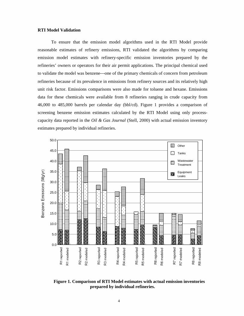
To ensure that the emission model algorithms used in the RTI Model provide

reasonable estimates of refinery emissions, RTI validated the algorithms by comparing

emission model estimates with refinery-specific emission inventories prepared by the

refineries’ owners or operators for their air permit applications. The principal chemical used

to validate the model was benzeneone of the primary chemicals of concern from petroleum

refineries because of its prevalence in emissions from refinery sources and its relatively high

unit risk factor. Emissions comparisons were also made for toluene and hexane. Emissions

data for these chemicals were available from 8 refineries ranging in crude capacity from

46,000 to 485,000 barrels per calendar day (bbl/cd). Figure 1 provides a comparison of

screening benzene emission estimates calculated by the RTI Model using only process-

capacity data reported in the Oil & Gas Journal (Stell, 2000) with actual emission inventory

estimates prepared by individual refineries.

Figure 1. Comparison of RTI Model estimates with actual emission inventories

prepared by individual refineries.

0.0

5.0

10.0

15.0

20.0

25.0

30.0

35.0

40.0

45.0

50.0

Equipment Leaks

Wastewater Treatment

Tanks

Other

5

In general, the RTI Model provided benzene emission estimates that were within a

factor of 2 of the reported emissions for each generalized emission source category (emission

estimates for toluene and hexane exhibited similar agreement with reported values). Emission

estimates for equipment leaks and wastewater treatment exhibited the best comparison with

the reported values.1

For the most part, the tank emission estimates did not appear to have a particular bias,

but the emission estimates for this source could vary widely from the reported emission

estimates. These variations are a direct result of the assumptions used in the RTI Model when

only process-capacity information is provided. For example, the tank emissions reported for

Refinery 4 are much higher than those projected by the model. This discrepancy is caused

predominately by emissions reported from three fixed-roof tanks at the refinery. The RTI

Model, when used with only process-capacity information, assumes that all tanks with

significant VOC content have floating roofs. These three fixed-roof tanks at Refinery 4 had a

significant VOC and benzene loading and therefore higher tank emissions than projected by

the RTI Model. On the other hand, the reported tank emissions for Refinery 5 are much lower

than those estimated by the model. Refinery 5 operates an aromatics unit that produces

toluene and xylene, but does not produce benzene as a product. The RTI Model, when used

with only process-capacity information, cannot distinguish among specific aromatics

produced in the aromatics unit. The default emission estimates are based on an aromatics unit

that produces three aromatic products (benzene, toluene, and xylene). The RTI Model

estimates roughly 5 Mg/yr of benzene emissions occur from the benzene product storage

tanks. By simply specifying the aromatics produced by the aromatics unit, the resulting tank

emissions for this refinery compare well with the reported values. These comparisons

indicate how site-specific detail can be incorporated into the RTI Model inputs to provide

more-refined emission estimates for a given refinery.

In every case, the RTI Model’s estimates for “other” sources are higher than the

reported emissions. The “other” sources include emissions from cooling towers, combustion

sources, flares, and product-loading operations. Emissions from these sources were not

always reported by the refineries in their permit applications. Therefore, it is uncertain if the

1 Refinery 4 did not report any benzene emissions from the wastewater treatment system; it is unclear if the RTI Model overestimated these emissions or if the refinery underreported them.

6

emission estimates for “other” sources were overestimated by the RTI Model or

underreported in these refinery emission inventories.

The RTI Model emission estimates for the overall refinery were within 30 percent of

the reported values for 5 of the 8 refineries and were within approximately 50 percent of the

reported values for all but 1 refinery. The emission estimates for Refinery 5 were off by a

factor of 2. As discussed previously, this discrepancy is largely due to the lack of benzene

product from the aromatics unit for this refinery. Although the tank emission estimates are

affected most significantly by the specification of which aromatics are produced in the

aromatics unit, the benzene emission estimates for some of the other emission sources (e.g.,

equipment leaks and wastewater treatment) are also reduced. By entering this one site-

specific factor into the model, the RTI Model’s estimated overall benzene emissions fall to

within 50 percent of the reported emissions for all of the refineries.

The model validation comparisons suggest that the RTI Model is a practical tool for

performing facility-wide emission inventories and developing emission estimates for use in

risk assessments. Site-specific information can easily be incorporated into the model to

provide more accurate emission estimates for a given refinery. The RTI Model outputs can

also be used to identify sources that are major contributors to a refinery’s air emissions, and

this information can help facility managers and operators target cost-effective emission-

reduction strategies.

The following case studies illustrate how the RTI Model has been applied to achieve a

variety of environmental goals. Although the case studies themselves are hypothetical, they

are based on data and characteristics adapted from an actual facility. All three case studies

use the same facility, Refinery X, to demonstrate model applications. Case Studies 1 and 2

illustrate how the RTI model can be used to identify sources that are significant contributors

to a refinery’s emissions or risk level. Case Study 1 shows how the modeling tool can be used

to identify primary sources of VOC emissions and identify effective emission-reduction

projects to meet the refinery’s emission-reduction goals. Case Study 2 shows how the RTI

Model can be used to assess risk. These two case studies provide a contrast between an

emission-reduction and a risk-reduction paradigm. For the same refinery, these two goals

target completely different emission sources, and consequently, different control strategies.

Case Study 3 shows how control-cost functions included within the RTI Model provide

7

preliminary cost estimates that can be used to evaluate the cost-effectiveness of alternative

control strategies.

Case Study 1. Detailed Refinery Analysis: VOC Emission-Reduction Goal

Introduction

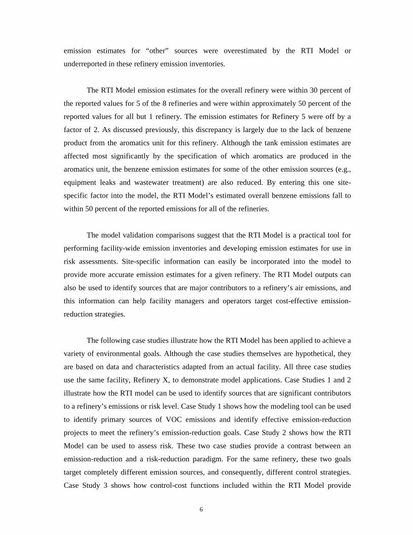
In this case study, Refinery X sought to reduce its VOC emissions by 50 percent to

meet ambient air standards. To achieve this 50 percent reduction in VOC emissions, the

refinery had to identify cost-effective control options. In general, the process operations at

Refinery X conform with the general assumptions used by the RTI model when estimating

emissions from process-capacity data (see Table 1 for process unit capacities for this

refinery). However, it has the following special features, which do not conform with the

general assumptions:

The facility has a few miscellaneous process vents (scrubber and stripper

overheads, distillation tower condensers/accumulators, flash/knock-out drums,

etc.) that have significant VOC emissions, but are uncontrolled.

The facility has 3 fixed-roof tanks that have significant VOC loadings.

The equalization basin in the facility’s wastewater treatment area is uncovered.

Table 1. Process Data for Refinery X

Process Unit Capacity (bbl/cd)

Crude 250,000 Vacuum Distillation 90,000 Coking 25,000 Catalytic Cracking 100,000 Catalytic Reforming 40,000 Catalytic Hydrotreating 110,000 Alkylation 40,000 Aromatics 15,000

8

Methods

The RTI Model was used to calculate emission estimates for this facility using the

process capacities presented in Table 1 and the RTI Model default emission estimates for

uncontrolled miscellaneous process vents. Additional emissions were estimated for the

uncovered equalization basin using the RTI-developed WATER9 emission model (U.S. EPA,

2001). Next, to develop the VOC emission estimates for the refinery, the constituent-specific

emission estimates provided by the RTI Model were summed for the volatile compounds.

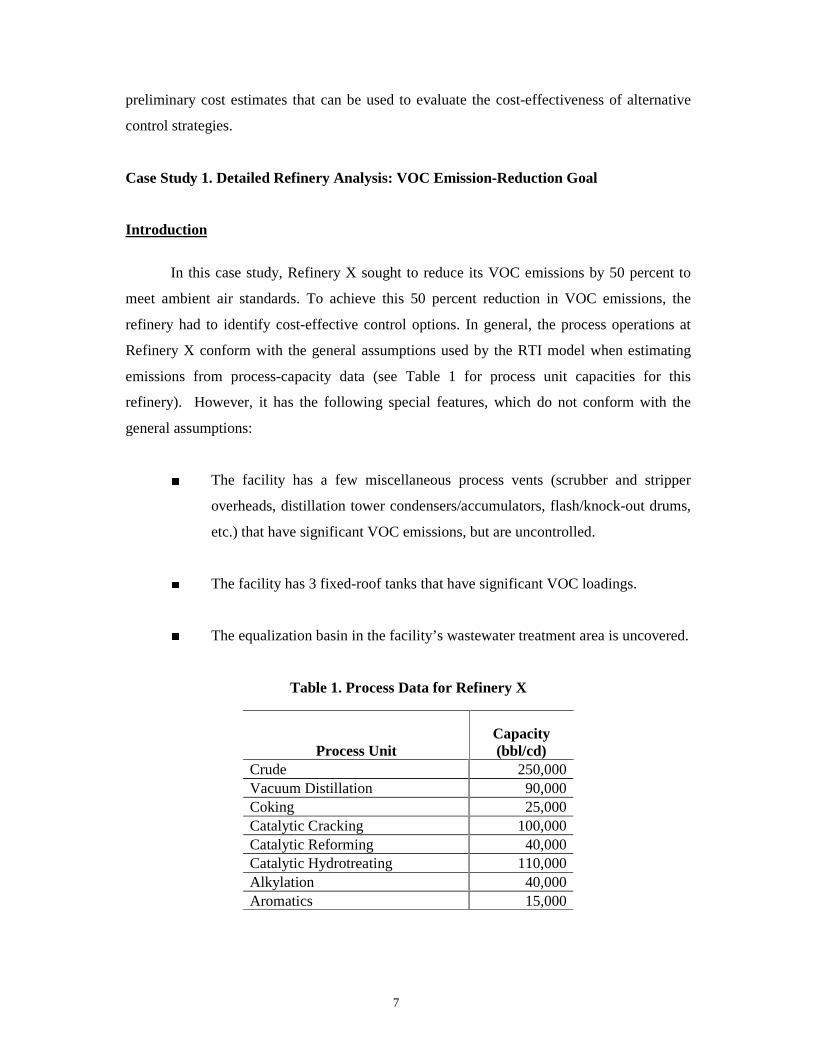
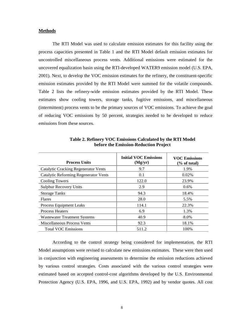
Table 2 lists the refinery-wide emission estimates provided by the RTI Model. These

estimates show cooling towers, storage tanks, fugitive emissions, and miscellaneous

(intermittent) process vents to be the primary sources of VOC emissions. To achieve the goal

of reducing VOC emissions by 50 percent, strategies needed to be developed to reduce

emissions from these sources.

Table 2. Refinery VOC Emissions Calculated by the RTI Model before the Emission-Reduction Project

Process Units Initial VOC Emissions

(Mg/yr) VOC Emissions

(% of total) Catalytic Cracking Regenerator Vents 9.7 1.9%

Catalytic Reforming Regenerator Vents 0.1 0.02%

Cooling Towers 122.0 23.9%

Sulphur Recovery Units 2.9 0.6%

Storage Tanks 94.3 18.4% Flares 28.0 5.5%

Process Equipment Leaks 114.1 22.3% Process Heaters 6.9 1.3%

Wastewater Treatment Systems 40.9 8.0%

Miscellaneous Process Vents 92.3 18.1%

Total VOC Emissions 511.2 100%

According to the control strategy being considered for implementation, the RTI

Model assumptions were revised to calculate new emissions estimates. These were then used

in conjunction with engineering assessments to determine the emission reductions achieved

by various control strategies. Costs associated with the various control strategies were

estimated based on accepted control-cost algorithms developed by the U.S. Environmental

Protection Agency (U.S. EPA, 1996, and U.S. EPA, 1992) and by vendor quotes. All cost

9

estimates were calculated in 2001 U.S. dollars; a VOC recovery credit of $0.16 per kilogram

of VOC recovered was used for all applicable emission sources.

Results

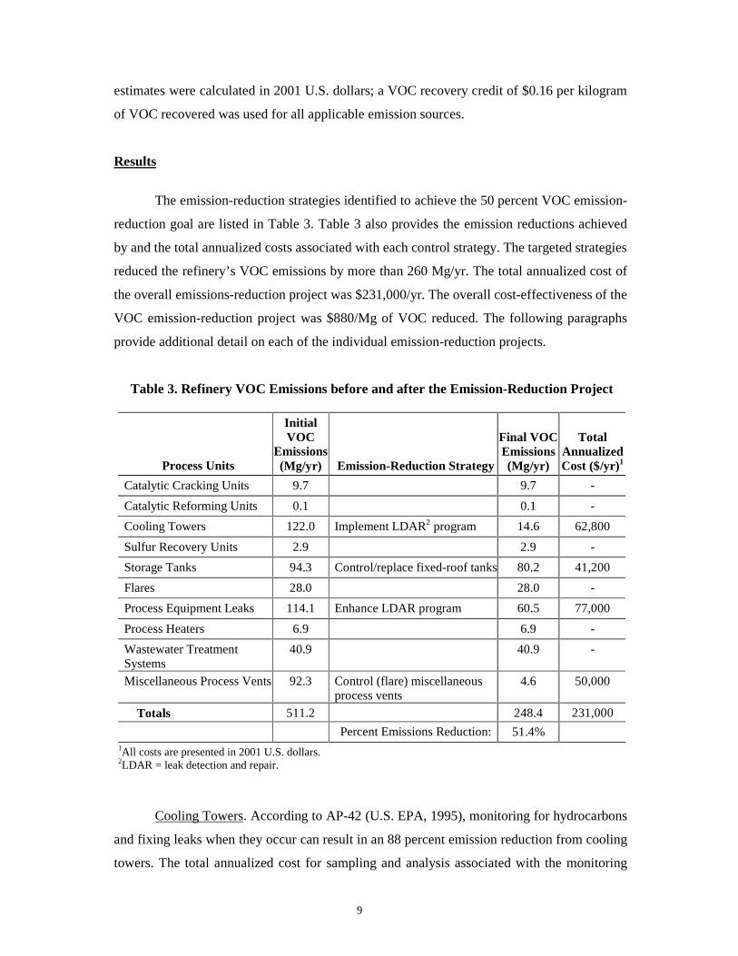
The emission-reduction strategies identified to achieve the 50 percent VOC emission-

reduction goal are listed in Table 3. Table 3 also provides the emission reductions achieved

by and the total annualized costs associated with each control strategy. The targeted strategies

reduced the refinery’s VOC emissions by more than 260 Mg/yr. The total annualized cost of

the overall emissions-reduction project was $231,000/yr. The overall cost-effectiveness of the

VOC emission-reduction project was $880/Mg of VOC reduced. The following paragraphs

provide additional detail on each of the individual emission-reduction projects.

Table 3. Refinery VOC Emissions before and after the Emission-Reduction Project

Process Units

Initial VOC

Emissions (Mg/yr) Emission-Reduction Strategy

Final VOC Emissions (Mg/yr)

Total Annualized Cost ($/yr)1

Catalytic Cracking Units 9.7 9.7 -

Catalytic Reforming Units 0.1 0.1 -

Cooling Towers 122.0 Implement LDAR2 program 14.6 62,800

Sulfur Recovery Units 2.9 2.9 -

Storage Tanks 94.3 Control/replace fixed-roof tanks 80.2 41,200

Flares 28.0 28.0 -

Process Equipment Leaks 114.1 Enhance LDAR program 60.5 77,000

Process Heaters 6.9 6.9 -

Wastewater Treatment Systems

40.9 40.9 -

Miscellaneous Process Vents 92.3 Control (flare) miscellaneous process vents

4.6 50,000

Totals 511.2 248.4 231,000

Percent Emissions Reduction: 51.4% 1All costs are presented in 2001 U.S. dollars. 2LDAR = leak detection and repair.

Cooling Towers. According to AP-42 (U.S. EPA, 1995), monitoring for hydrocarbons

and fixing leaks when they occur can result in an 88 percent emission reduction from cooling

towers. The total annualized cost for sampling and analysis associated with the monitoring

10

protocol was $48,000/yr;2 additional cost of labor and parts for repairing the leaks was

estimated at $32,000/yr. The product recovery credit was estimated at $17,200/yr. Therefore,

the net costs associated with a quarterly leak detection and repair (LDAR) program for heat

exchangers was $62,800/yr, or $580/Mg VOC reduced.

Storage Tanks. Tank emission estimates are based on data correlations for typical tank

farms that predominately employ floating-roof tanks. The RTI Model estimates the relative

amounts of different types of liquid stored (either crude, aromatics, light distillates, or heavy

distillates) based on the types and capacities of the processes used by the refinery. Once

storage tanks are identified as a potential source of concern, more-detailed modeling of the

tank farm emissions is made using site-specific data for individual tanks, to provide improved

emission estimates and to identify appropriate control scenarios.

For the most part, Refinery X controls storage tank emissions using floating-roof

tanks, but it also employs three 30-meter diameter fixed-roof tanks. Using site-specific data,

the TANKS 4.09 software program (U.S. EPA, 1999) was used to provide tank-specific

emission estimates for these fixed-roof tanks. The three tanks were estimated to contribute

more than 15 Mg/yr to the VOC emissions total. Upgrading these tanks with internal floating

roofs or venting the fixed-roof tanks to a common refrigerated condenser were both projected

to reduce VOC emissions by 95 percent or more. The total annualized cost for upgrading the

three tanks with internal floating roofs was estimated at $43,500/yr; the total annualized cost

for installing a refrigerated condenser and venting the three fixed-roof tanks to the condenser

was estimated at $143,000/yr. An annual credit of $2,300 was realized from the reduced

VOC loss (or VOC recovered) with either option. Based on these costs, the control strategy

of upgrading the three fixed-roof tanks with internal floating roofs was selected. Therefore,

the net total annualized cost of the storage-tank control option was $41,200/yr, or the cost-

effectiveness of the storage tank controls was $2,920/Mg VOC reduced.

Equipment Leaks. LDAR programs must define the frequency of monitoring, the

value above which the equipment component is defined to be leaking, and the acceptable

percentage of leaking components. The latter two values are optional input parameters to the

RTI Model equipment leak algorithm and can be used to assess the emission reduction

2 All dollar amounts are in 2001 U.S. dollars.

11

obtainable through different LDAR programs. Regulatory requirements often determine the

frequency of monitoring, but a proactive LDAR program should vary monitoring frequency

based on the monitoring results. If equipment leak criteria are exceeded, a higher frequency

of monitoring is needed; if equipment leak criteria are consistently met, less-frequent

monitoring is acceptable. For Refinery X, performing an LDAR that reduced the allowable

percentage of leaking components by a factor of 2 (maintaining the current leak definition of

10,000 ppmv) was projected to reduce VOC emissions by 47 percent. The existing LDAR at

the refinery used semiannual inspections. The proactive LDAR program used quarterly

inspections and reverted back to semiannual monitoring when the percentage of leaking

equipment fell below target levels for one year (four consecutive monitoring events). The

added annual cost associated with the more stringent LDAR program was estimated at

$85,600/yr and included costs for both more-frequent monitoring and more-frequent repairs.

A recovery credit of $8,600/yr was realized from lower product loss through leaking

equipment. Therefore, the net annual cost was $77,000/yr, or $1,440/Mg VOC reduced.

Miscellaneous Process Vents. Miscellaneous process vents include distillation tower

condensers/accumulators, flash/knock-out drums, scrubber and stripper overheads, and vents

from blowdown condensers/accumulators. Large miscellaneous process vents are generally

controlled by a flare or by venting the gas to the refinery fuel gas system, depending on the

vent stream composition. However, small miscellaneous process vents may vent directly to

the atmosphere. The uncontrolled miscellaneous vents are characterized based on size, VOC

content, and proximity to an existing flare system to identify specific vent streams with a

sufficient heating value that could be easily controlled. For Refinery X, approximately 90

Mg/yr of the VOC emissions were attributable to uncontrolled process vents that were

amenable to control. The VOC control efficiency of flaring was assumed to be 98 percent.

Costs associated with the project included knock-out drums, piping, and one 2.5-centemeter

diameter flare. Total annualized costs for the system were estimated at $50,000/yr, or

$570/Mg VOC controlled.

The refinery-wide emission inventory provided by the RTI Model enabled primary

sources of VOC emissions to be identified, which then allowed appropriate emission-

reduction strategies to be targeted to achieve the desired goal. In the end, total VOC

emissions were reduced by more than 260 Mg/yr at a total annualized cost of $231,000 (see

12

Table 3). The overall cost-effectiveness of the VOC emission-reduction project was $880/Mg

VOC reduced.

Case Study 2. Detailed Refinery Analysis: Risk-Reduction Goal

Introduction

In this case study, Refinery X was evaluated to show how the RTI Model could be

used to assess risk. This time, the refinery sought to identify cost-effective control options

for reducing its cancer risk to humans to below 10-6. The refinery emissions were the same as

in Case Study 1, but the focus was now the potency of the individual constituents emitted and

the proximity of the emission sources to the most-exposed individual (MEI). The RTI Model

was developed specifically to output emissions data and source characterization data for input

into a risk assessment model. RTI has the capability to perform multipathway risk

assessments using its multimedia, multipathway, multireceptor risk assessment (3MRA)

model and its multipathway risk assessment tool (MPRAT). These modeling tools were

developed in conjunction with EPA and have been subject to peer review. For this case study,

however, only inhalation exposure was evaluated.

Methods

The Industrial Source Complex Short-Term Model, version 3 (ISCST3), was used to

calculate dispersion factors based on a unit emission rate (1 g/m2/sec for area sources and

1 g/sec for point sources). This model is a standard, EPA-approved model for predicting

atmospheric dispersion and deposition of chemical species up to 50 km from the source.

Cancer risks were calculated using the health benchmarks from EPA’s Integrated Risk

Information System (IRIS).

In modeling emissions and dispersion from the tank farm, tanks were modeled

together as one large area source rather than separately as individual sources. Similarly,

process fugitives (equipment leaks) were treated as one large area source within the

processing area of the refinery. Wastewater treatment emissions were divided into two area

sources: one area source within the processing area of the refinery for the wastewater

collection system and one area source for all wastewater treatment units in the wastewater

13

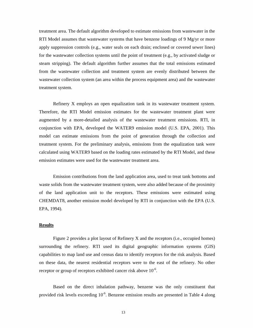
treatment area. The default algorithm developed to estimate emissions from wastewater in the

RTI Model assumes that wastewater systems that have benzene loadings of 9 Mg/yr or more

apply suppression controls (e.g., water seals on each drain; enclosed or covered sewer lines)

for the wastewater collection systems until the point of treatment (e.g., by activated sludge or

steam stripping). The default algorithm further assumes that the total emissions estimated

from the wastewater collection and treatment system are evenly distributed between the

wastewater collection system (an area within the process equipment area) and the wastewater

treatment system.

Refinery X employs an open equalization tank in its wastewater treatment system.

Therefore, the RTI Model emission estimates for the wastewater treatment plant were

augmented by a more-detailed analysis of the wastewater treatment emissions. RTI, in

conjunction with EPA, developed the WATER9 emission model (U.S. EPA, 2001). This

model can estimate emissions from the point of generation through the collection and

treatment system. For the preliminary analysis, emissions from the equalization tank were

calculated using WATER9 based on the loading rates estimated by the RTI Model, and these

emission estimates were used for the wastewater treatment area.

Emission contributions from the land application area, used to treat tank bottoms and

waste solids from the wastewater treatment system, were also added because of the proximity

of the land application unit to the receptors. These emissions were estimated using

CHEMDAT8, another emission model developed by RTI in conjunction with the EPA (U.S.

EPA, 1994).

Results

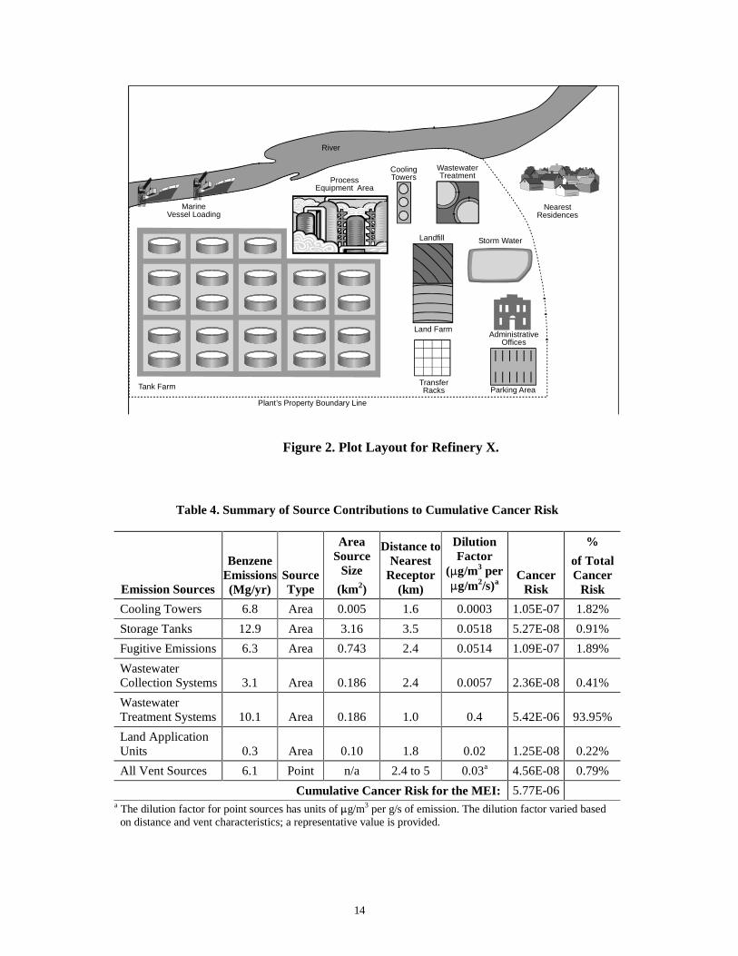
Figure 2 provides a plot layout of Refinery X and the receptors (i.e., occupied homes)

surrounding the refinery. RTI used its digital geographic information systems (GIS)

capabilities to map land use and census data to identify receptors for the risk analysis. Based

on these data, the nearest residential receptors were to the east of the refinery. No other

receptor or group of receptors exhibited cancer risk above 10-6.

Based on the direct inhalation pathway, benzene was the only constituent that

provided risk levels exceeding 10-6. Benzene emission results are presented in Table 4 along

14

Figure 2. Plot Layout for Refinery X.

Table 4. Summary of Source Contributions to Cumulative Cancer Risk

Emission Sources

Benzene Emissions (Mg/yr)

Source Type

Area Source

Size

(km2)

Distance to Nearest

Receptor (km)

Dilution Factor

(�g/m3 per �g/m2/s)a

Cancer Risk

%

of Total Cancer

Risk

Cooling Towers 6.8 Area 0.005 1.6 0.0003 1.05E-07 1.82%

Storage Tanks 12.9 Area 3.16 3.5 0.0518 5.27E-08 0.91%

Fugitive Emissions 6.3 Area 0.743 2.4 0.0514 1.09E-07 1.89%

Wastewater Collection Systems 3.1 Area 0.186 2.4 0.0057 2.36E-08 0.41%

Wastewater Treatment Systems 10.1 Area 0.186 1.0 0.4 5.42E-06 93.95%

Land Application Units 0.3 Area 0.10 1.8 0.02 1.25E-08 0.22%

All Vent Sources 6.1 Point n/a 2.4 to 5 0.03a 4.56E-08 0.79%

Cumulative Cancer Risk for the MEI: 5.77E-06 a The dilution factor for point sources has units of �g/m3 per g/s of emission. The dilution factor varied based on distance and vent characteristics; a representative value is provided.

LandFarm

TransferRacks

Storm Water

AdministrativeOffices

Parking Area

Plant’s Property Boundary Line

CoolingTowers

WastewaterTreatment

River

MarineVessel Loading

Tank Farm

Landfill

Land Farm

ProcessEquipment Area

NearestResidences

15

with the distance from the emission source to the nearest receptor, or more specifically, to the

MEI. Table 4 also provides some source characterization data and the contribution made to

the total risk by each emission source.

The risk-reduction paradigm had a completely different focus than the VOC emission-

reduction paradigm. In this case, the wastewater treatment system completely dominated the

risk results because of the proximity of the wastewater treatment system to the residential

neighborhood. To reduce the cancer risk incidence to the MEI to less than 10-6, the benzene

emissions from the wastewater treatment system had to be reduced to 1.21 Mg/yr or less, an

88 percent emission reduction.

Based on the site-specific benzene concentration in the inlet wastewater and more-

detailed modeling of the wastewater treatment system with WATER9, it was determined that

covering the equalization basin would not sufficiently reduce the benzene emissions from the

wastewater treatment system. Even when using site-specific biodegradation rate constants in

WATER9, the existing wastewater treatment system could not sufficiently reduce the

emissions below the desired levels.

The alternatives remaining were to convert the existing wastewater treatment system

to a powdered activated carbon treatment (PACT) system or to install a steam stripper. Based

on the Henry’s law constant for benzene (a measure of the volatility of a compound in dilute

aqueous solution), the removal efficiency of the steam stripper for benzene should exceed

98 percent. As such, the steam stripper was considered the more reliable technology for this

application to achieve the desired level of emissions control. The capital investment and

annual operating costs to pretreat all of the refinery wastewater (roughly 7,500 m3/day) were

estimated at $4.5 million and $2.75 million, respectively.

In an effort to reduce the project costs, a third alternative was devised to segregate

certain wastewater streams from the crude unit, the coker, the reformer, and the aromatics

unit for pretreatment with the steam stripper, and to install a cover on the equalization basin.

Based on the RTI Model estimates, these units accounted for roughly 75 percent of the

refinery’s benzene loading to the system in less than one-half the volume of wastewater

currently generated by the refinery. The emission reductions effected by a steam stripper for

these wastewater streams, coupled with the emission reductions achievable by covering the

16

equalization basin, achieved the necessary 88 percent reduction in benzene emissions from

the wastewater treatment system. Although the capital investment of this third alternative was

roughly equivalent to the cost of the large steam stripper, the annual operating costs were

reduced by $1.4 million compared to steam stripping all of the refinery’s wastewater.

Application of the RTI Model helped to identify a more cost-effective means of achieving the

desired risk-reduction goal.

Case Study 3. Compliance with Particulate Matter Standards

Introduction

In this case study, Refinery X sought to identify cost-effective regulatory compliance

strategies for the fluid catalytic cracking unit (FCCU) catalyst regenerator vent. The FCCU

catalyst regenerator burns off coke that is deposited on the catalyst during the cracking

process. The FCCU catalyst regenerator is the primary source of particulate matter (PM)

emissions from a refinery; nickel (Ni) emissions associated with this vent stream are a

potential concern with respect to human risk. The FCCU catalyst regenerator may also be a

significant contributor to sulfur oxide (SOx) emissions. Depending on the location of the

refinery, the refinery may be subject to PM, Ni, and/or SOx emission limits from the FCCU

catalyst regenerator vent or subject to PM and SO2 concentration limits at the fence line. This

case study specifically evaluated alternative control strategies with respect to meeting a PM

emission limit of 50 mg/m3 from the FCCU catalyst regenerator vent.

Given the premise of this case study, the RTI Model was not needed to identify the

primary source of emissions to target emission-reduction strategies. Instead, the regulatory

statute dictated the emission source to be controlled. For the most part, cost analyses are

performed for specific applications using site-specific parameters. Some generalized costing

algorithms are, however, included in the RTI Model. This case study also serves to illustrate

how costing algorithms are used in the RTI Model to provide preliminary cost estimates.

Refinery X’s FCCU, which has a capacity of 100,000 bbls/cd, is a complete

combustion unit with an average coke burn rate at capacity of 28 Mg/hr (62,000 lbs/hr). The

FCCU catalyst regenerator flow rate was estimated to be 340,000 standard m3/hr at full

capacity (standard conditions used here were 1 atmosphere and 20°C). Current exhaust-

17

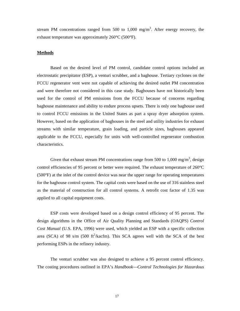
stream PM concentrations ranged from 500 to 1,000 mg/m3. After energy recovery, the

exhaust temperature was approximately 260°C (500°F).

Methods

Based on the desired level of PM control, candidate control options included an

electrostatic precipitator (ESP), a venturi scrubber, and a baghouse. Tertiary cyclones on the

FCCU regenerator vent were not capable of achieving the desired outlet PM concentration

and were therefore not considered in this case study. Baghouses have not historically been

used for the control of PM emissions from the FCCU because of concerns regarding

baghouse maintenance and ability to endure process upsets. There is only one baghouse used

to control FCCU emissions in the United States as part a spray dryer adsorption system.

However, based on the application of baghouses in the steel and utility industries for exhaust

streams with similar temperature, grain loading, and particle sizes, baghouses appeared

applicable to the FCCU, especially for units with well-controlled regenerator combustion

characteristics.

Given that exhaust stream PM concentrations range from 500 to 1,000 mg/m3, design

control efficiencies of 95 percent or better were required. The exhaust temperature of 260°C

(500°F) at the inlet of the control device was near the upper range for operating temperatures

for the baghouse control system. The capital costs were based on the use of 316 stainless steel

as the material of construction for all control systems. A retrofit cost factor of 1.35 was

applied to all capital equipment costs.

ESP costs were developed based on a design control efficiency of 95 percent. The

design algorithms in the Office of Air Quality Planning and Standards (OAQPS) Control

Cost Manual (U.S. EPA, 1996) were used, which yielded an ESP with a specific collection

area (SCA) of 98 s/m (500 ft2/kacfm). This SCA agrees well with the SCA of the best

performing ESPs in the refinery industry.

The venturi scrubber was also designed to achieve a 95 percent control efficiency.

The costing procedures outlined in EPA’s HandbookControl Technologies for Hazardous

18

Air Pollutants (U.S. EPA, 1991) were used to develop costs for venturi scrubbers. The

projected pressure drop across the scrubber was estimated to be 30" of water.

The baghouse is anticipated to achieve a PM removal efficiency of 99 percent or

higher. The baghouse was designed as a modular pulse-jet unit with an air-to-cloth ratio of 55

m/hr (3 ft/min). Because of the operating temperature of the control system, fiberglass was

selected as the fabric material for the filter bags. Costing procedures followed guidance

presented in the Control Cost Manual (U.S. EPA, 1996).

Given the control device design parameters, control costs were developed for 6

different exhaust flow rates from 25,000 to 340,000 standard m3/hr. Control-cost curves were

developed using linear regression analyses for the total capital investment and the annual

operating costs.

Results

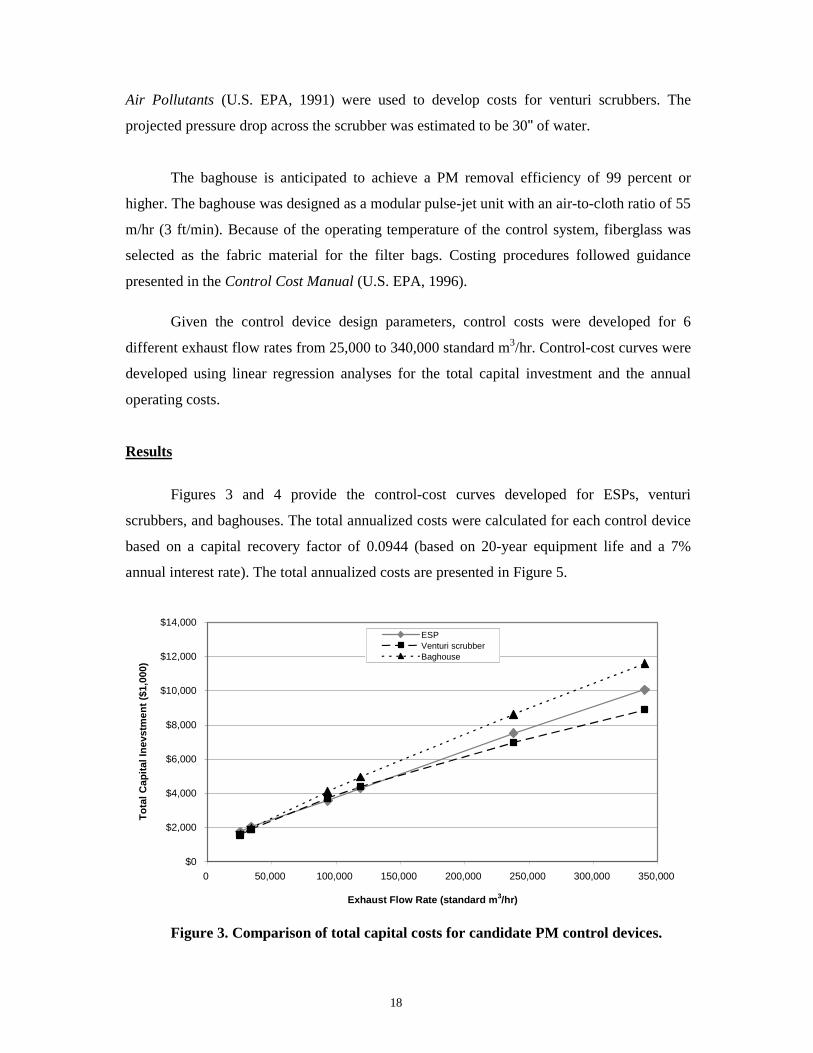
Figures 3 and 4 provide the control-cost curves developed for ESPs, venturi

scrubbers, and baghouses. The total annualized costs were calculated for each control device

based on a capital recovery factor of 0.0944 (based on 20-year equipment life and a 7%

annual interest rate). The total annualized costs are presented in Figure 5.

Figure 3. Comparison of total capital costs for candidate PM control devices.

$0

$2,000

$4,000

$6,000

$8,000

$10,000

$12,000

$14,000

0 50,000 100,000 150,000 200,000 250,000 300,000 350,000

Exhaust Flow Rate (standard m3/hr)

To

tal C

apit

al In

evst

men

t ($

1,00

0)

ESPVenturi scrubberBaghouse

19

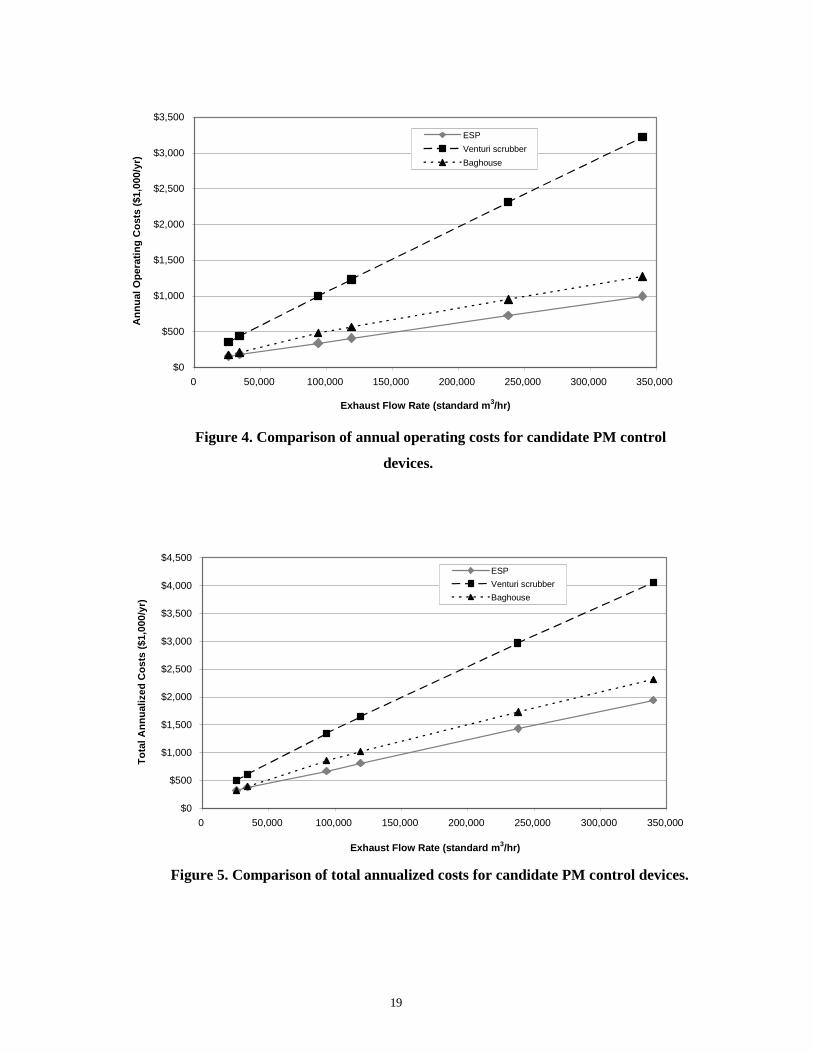
Figure 4. Comparison of annual operating costs for candidate PM control

devices.

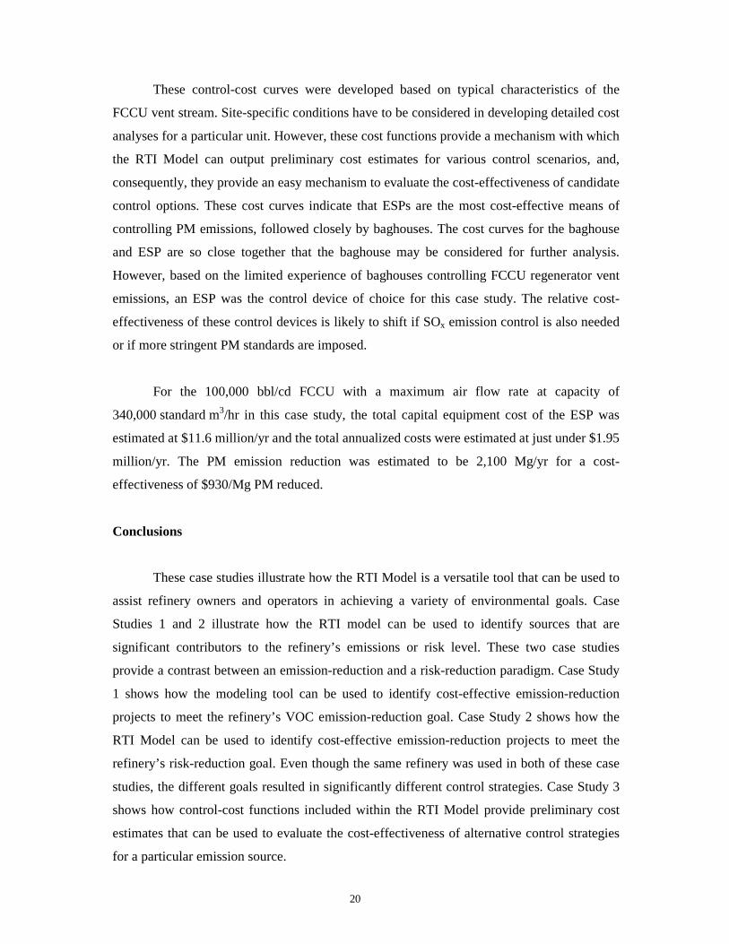
Figure 5. Comparison of total annualized costs for candidate PM control devices.

$0

$500

$1,000

$1,500

$2,000

$2,500

$3,000

$3,500

$4,000

$4,500

0 50,000 100,000 150,000 200,000 250,000 300,000 350,000

Exhaust Flow Rate (standard m3/hr)

To

tal A

nn

ual

ized

Co

sts

($1,

000/

yr)

ESP

Venturi scrubber

Baghouse

$0

$500

$1,000

$1,500

$2,000

$2,500

$3,000

$3,500

0 50,000 100,000 150,000 200,000 250,000 300,000 350,000

Exhaust Flow Rate (standard m3/hr)

An

nu

al O

per

atin

g C

ost

s ($

1,00

0/yr

)ESP

Venturi scrubber

Baghouse

20

These control-cost curves were developed based on typical characteristics of the

FCCU vent stream. Site-specific conditions have to be considered in developing detailed cost

analyses for a particular unit. However, these cost functions provide a mechanism with which

the RTI Model can output preliminary cost estimates for various control scenarios, and,

consequently, they provide an easy mechanism to evaluate the cost-effectiveness of candidate

control options. These cost curves indicate that ESPs are the most cost-effective means of

controlling PM emissions, followed closely by baghouses. The cost curves for the baghouse

and ESP are so close together that the baghouse may be considered for further analysis.

However, based on the limited experience of baghouses controlling FCCU regenerator vent

emissions, an ESP was the control device of choice for this case study. The relative cost-

effectiveness of these control devices is likely to shift if SOx emission control is also needed

or if more stringent PM standards are imposed.

For the 100,000 bbl/cd FCCU with a maximum air flow rate at capacity of

340,000 standard m3/hr in this case study, the total capital equipment cost of the ESP was

estimated at $11.6 million/yr and the total annualized costs were estimated at just under $1.95

million/yr. The PM emission reduction was estimated to be 2,100 Mg/yr for a cost-

effectiveness of $930/Mg PM reduced.

Conclusions

These case studies illustrate how the RTI Model is a versatile tool that can be used to

assist refinery owners and operators in achieving a variety of environmental goals. Case

Studies 1 and 2 illustrate how the RTI model can be used to identify sources that are

significant contributors to the refinery’s emissions or risk level. These two case studies

provide a contrast between an emission-reduction and a risk-reduction paradigm. Case Study

1 shows how the modeling tool can be used to identify cost-effective emission-reduction

projects to meet the refinery’s VOC emission-reduction goal. Case Study 2 shows how the

RTI Model can be used to identify cost-effective emission-reduction projects to meet the

refinery’s risk-reduction goal. Even though the same refinery was used in both of these case

studies, the different goals resulted in significantly different control strategies. Case Study 3

shows how control-cost functions included within the RTI Model provide preliminary cost

estimates that can be used to evaluate the cost-effectiveness of alternative control strategies

for a particular emission source.

21

The RTI Model is a unique tool that can be used with a minimum of process data to

develop emission inventories, identify primary sources of chemical-specific emissions, and

provide input for refinery risk assessments. Additional site-specific process information can

be entered into the model to provide more accurate emission inventories or risk assessments.

When combined with control-cost analyses, the RTI Model provides an excellent tool for

developing cost-effective control strategies.

References

Stell, J. 2000. 2000 Worldwide Refining Survey. Survey Editor. Oil & Gas Journal,

December 18, 2000. pp. 66-120.

U.S. EPA (Environmental Protection Agency). 1991. HandbookControl Technologies for

Hazardous Air Pollutants. Publication No. EPA/625/6-91/014. Office of Research and

Development, Washington, DC.

U.S. EPA (Environmental Protection Agency). 1992. Hazardous Air Pollutant Emissions

from Process Units in the Snythetic Organic Chemical Manufacturing Industry –

Background Information for Proposed Standards. EPA-453/D-92-016b. Office of Air

Quality Planning and Standards, Research Triangle Park, NC.

U.S. EPA (Environmental Protection Agency). 1994. Air Emissions Models for Waste and

Wastewater. EPA-453/R-94-080A. Office of Air Quality Planning and Standards,

Research Triangle Park, NC.

U.S. EPA (Environmental Protection Agency). 1995. Compilation of Air Pollutant Emission

Factors. AP-42. Office of Air Quality Planning and Standards, Research Triangle

Park, NC.

U.S. EPA (Environmental Protection Agency). 1996. OAQPS Control Cost Manual.

Publication No. EPA 453/B-96-001. Office of Air Quality Planning and Standards,

Research Triangle Park, NC.

22

U.S. EPA (Environmental Protection Agency). 1999. User’s Guide to TANKSStorage Tank

Emissions Calculation Software, Version 4.0. Office of Air Quality Planning and

Standards, Research Triangle Park, NC.

U.S. EPA (Environmental Protection Agency). 2001. User’s Guide for WATER9 Software,

Version 1.0.0. Office of Air Quality Planning and Standards, Research Triangle Park,

NC.