Successful transient EM survey in the North Sea at 100 m water depth Anton Ziolkowski*, David Wright, Guy Hall, and Craig Clarke, Petroleum Geo-Services, 40 Sciennes, Edinburgh EH9 1NJ, United Kingdom. Summary We describe the acquisition, processing, and interpretation of a successful transient electromagnetic survey acquired in water 100 m deep in the North Sea with a 30-channel sea- floor receiver cable and bipole current source. The equipment was deployed along several lines to record data with very dense subsurface coverage: source-receiver offsets in the range 1,000 – 6,000 m with 200 m increments and mid-points every 100 m. Data quality was appraised and processed in real time. A special feature of the processing was removal of the air wave, which allowed the data to be inverted for subsurface resistivities using tried and tested algorithms. We present the results, revealing a promising target, and step-by-step processing and inversion of the data. Introduction The conventional deep-water controlled-source EM exploration method was developed by the academic community (Cox, 1981; Cox et al., 1986; Sinha et al., 1990; Constable and Cox, 1996). The method uses multi- component EM receiver nodes on the sea floor and a dipole current source, towed just above the sea floor, that transmits a continuous periodic signal, typically a square wave. In the last few years this method has been applied to hydrocarbon exploration (Eidismo et al., 2002; Srnka et al., 2005; Constable and Srnka, 2007). It is well known that in water depths less than about 300 m the measurements are dominated by electromagnetic coupling between the atmosphere and the underlying geology. This is known as the shallow-water or airwave problem and makes interpretation of the data for sub-sea resistivity variations very difficult. Citing ideas proposed by Edwards (1997) and Scholl and Edwards (2007), Weiss (2007) argued that the air wave problem becomes tractable if a transient source signal, with a beginning and an end, is used instead of a continuous square wave. Wright et al. (2002, 2005) and Ziolkowski et al. (2007) describe the multi-transient EM method. The essence of the method is to obtain the complete impulse response of the earth for a current dipole source and an in-line receiver measuring the electric field, and to invert the impulse response for subsurface resistivity variations. In practice data are collected using geometries similar to 2D seismic reflection, with a source and line of receivers moving along the survey line, such that a regular grid of impulse responses is obtained in Common-Mid-Point (CMP) versus offset coordinates. In the land case the air wave is an impulse that arrives before the earth response. That is, the air wave is completely separable from the earth response. As Weiss (2007) points out, such a clear separation of “air” and “geology” signatures is more complicated in shallow- water environments. Ziolkowski and Wright (2007) addressed this issue. They pointed out that while the air wave decays with source- receiver offset r as 1/r 3 , the earth response decays as 1/r 5 . Therefore at large enough offset the air wave can be measured independently of the earth response and then used in a scheme to remove it from shorter-offset data. In their scheme an inverse filter was found for the air wave. Application of this filter to the shorter offset data compressed the air wave to an impulse, which was then cut out of the data. Convolution of the resulting data with the measured air wave resulted in an impulse response from which the air wave had been removed This paper describes the acquisition, processing, and inversion of shallow-water multi-transient EM data. Data Acquisition Figure 1: Showing deployment of sea-bottom receiver cable from one vessel and deployment of the bipole current source from a second vessel. Both vessels needed to hold their positions and had dynamic positioning. Figure 1 shows a schematic of the marine setup. The current bipole source consisted of two electrodes 200 m apart buoyed 2 m off the sea floor, and to which a pseudo- random binary sequence (PRBS) was applied, switching between +700A and -700A. A PRBS is a sequence that switches between two levels at pseudo-random multiples of some basic time interval Δt. Δt was varied for different offset ranges. The actual source current was not a perfect PRBS and was measured and then transmitted to the receiver vessel for data quality control and deconvolution. The observer on the receiver vessel controlled the source transmission. Source Receiver Buo 667 SEG Las Vegas 2008 Annual Meeting 667 Downloaded 01/01/15 to 77.99.219.105. Redistribution subject to SEG license or copyright; see Terms of Use at http://library.seg.org/
Transcript
Successful transient EM survey in the North Sea at 100 m water depth Anton Ziolkowski*, David Wright, Guy Hall, and Craig Clarke, Petroleum Geo-Services, 40 Sciennes, Edinburgh EH9 1NJ, United Kingdom. Summary
We describe the acquisition, processing, and interpretation of a successful transient electromagnetic survey acquired in water 100 m deep in the North Sea with a 30-channel sea-floor receiver cable and bipole current source. The equipment was deployed along several lines to record data with very dense subsurface coverage: source-receiver offsets in the range 1,000 – 6,000 m with 200 m increments and mid-points every 100 m. Data quality was appraised and processed in real time. A special feature of the processing was removal of the air wave, which allowed the data to be inverted for subsurface resistivities using tried and tested algorithms. We present the results, revealing a promising target, and step-by-step processing and inversion of the data.
Introduction The conventional deep-water controlled-source EM exploration method was developed by the academic community (Cox, 1981; Cox et al., 1986; Sinha et al., 1990; Constable and Cox, 1996). The method uses multi-component EM receiver nodes on the sea floor and a dipole current source, towed just above the sea floor, that transmits a continuous periodic signal, typically a square wave. In the last few years this method has been applied to hydrocarbon exploration (Eidismo et al., 2002; Srnka et al., 2005; Constable and Srnka, 2007). It is well known that in water depths less than about 300 m the measurements are dominated by electromagnetic coupling between the atmosphere and the underlying geology. This is known as the shallow-water or airwave problem and makes interpretation of the data for sub-sea resistivity variations very difficult. Citing ideas proposed by Edwards (1997) and Scholl and Edwards (2007), Weiss (2007) argued that the air wave problem becomes tractable if a transient source signal, with a beginning and an end, is used instead of a continuous square wave. Wright et al. (2002, 2005) and Ziolkowski et al. (2007) describe the multi-transient EM method. The essence of the method is to obtain the complete impulse response of the earth for a current dipole source and an in-line receiver measuring the electric field, and to invert the impulse response for subsurface resistivity variations. In practice data are collected using geometries similar to 2D seismic reflection, with a source and line of receivers moving along the survey line, such that a regular grid of impulse
responses is obtained in Common-Mid-Point (CMP) versus offset coordinates. In the land case the air wave is an impulse that arrives before the earth response. That is, the air wave is completely separable from the earth response. As Weiss (2007) points out, such a clear separation of “air” and “geology” signatures is more complicated in shallow-water environments. Ziolkowski and Wright (2007) addressed this issue. They pointed out that while the air wave decays with source-receiver offset r as 1/r3, the earth response decays as 1/r5. Therefore at large enough offset the air wave can be measured independently of the earth response and then used in a scheme to remove it from shorter-offset data. In their scheme an inverse filter was found for the air wave. Application of this filter to the shorter offset data compressed the air wave to an impulse, which was then cut out of the data. Convolution of the resulting data with the measured air wave resulted in an impulse response from which the air wave had been removed This paper describes the acquisition, processing, and inversion of shallow-water multi-transient EM data. Data Acquisition
Figure 1: Showing deployment of sea-bottom receiver
cable from one vessel and deployment of the bipole current source from a second vessel. Both vessels needed to hold their positions and had dynamic positioning.
Figure 1 shows a schematic of the marine setup. The current bipole source consisted of two electrodes 200 m apart buoyed 2 m off the sea floor, and to which a pseudo-random binary sequence (PRBS) was applied, switching between +700A and -700A. A PRBS is a sequence that switches between two levels at pseudo-random multiples of some basic time interval Δt. Δt was varied for different offset ranges. The actual source current was not a perfect PRBS and was measured and then transmitted to the receiver vessel for data quality control and deconvolution. The observer on the receiver vessel controlled the source transmission.
Source Receiver
Buo
667SEG Las Vegas 2008 Annual Meeting
Main Menu
667
Dow
nloa
ded
01/0
1/15
to 7
7.99
.219
.105
. Red
istr
ibut
ion
subj
ect t
o SE
G li
cens
e or
cop
yrig
ht; s
ee T
erm
s of
Use
at h
ttp://
libra
ry.s
eg.o
rg/
Successful transient EM survey in the North Sea at 100 m water depth
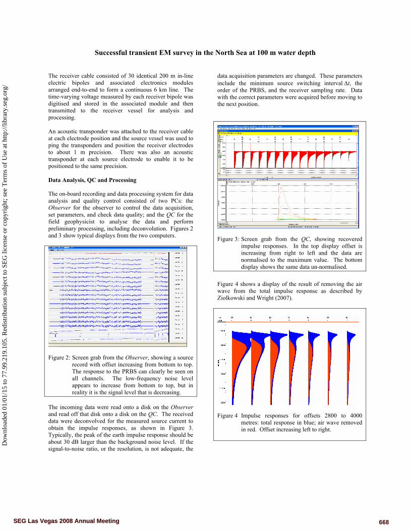
The receiver cable consisted of 30 identical 200 m in-line electric bipoles and associated electronics modules arranged end-to-end to form a continuous 6 km line. The time-varying voltage measured by each receiver bipole was digitised and stored in the associated module and then transmitted to the receiver vessel for analysis and processing. An acoustic transponder was attached to the receiver cable at each electrode position and the source vessel was used to ping the transponders and position the receiver electrodes to about 1 m precision. There was also an acoustic transponder at each source electrode to enable it to be positioned to the same precision. Data Analysis, QC and Processing The on-board recording and data processing system for data analysis and quality control consisted of two PCs: the Observer for the observer to control the data acquisition, set parameters, and check data quality; and the QC for the field geophysicist to analyse the data and perform preliminary processing, including deconvolution. Figures 2 and 3 show typical displays from the two computers.
Figure 2: Screen grab from the Observer, showing a source
record with offset increasing from bottom to top. The response to the PRBS can clearly be seen on all channels. The low-frequency noise level appears to increase from bottom to top, but in reality it is the signal level that is decreasing.
The incoming data were read onto a disk on the Observer and read off that disk onto a disk on the QC. The received data were deconvolved for the measured source current to obtain the impulse responses, as shown in Figure 3. Typically, the peak of the earth impulse response should be about 30 dB larger than the background noise level. If the signal-to-noise ratio, or the resolution, is not adequate, the
data acquisition parameters are changed. These parameters include the minimum source switching interval Δt, the order of the PRBS, and the receiver sampling rate. Data with the correct parameters were acquired before moving to the next position.
Figure 3: Screen grab from the QC, showing recovered
impulse responses. In the top display offset is increasing from right to left and the data are normalised to the maximum value. The bottom display shows the same data un-normalised.
Figure 4 shows a display of the result of removing the air wave from the total impulse response as described by Ziolkowski and Wright (2007).
Figure 4 Impulse responses for offsets 2800 to 4000
metres: total response in blue; air wave removed in red. Offset increasing left to right.
668SEG Las Vegas 2008 Annual Meeting
Main Menu
668
Dow
nloa
ded
01/0
1/15
to 7
7.99
.219
.105
. Red
istr
ibut
ion
subj
ect t
o SE
G li
cens
e or
cop
yrig
ht; s
ee T
erm
s of
Use
at h
ttp://
libra
ry.s
eg.o
rg/
Successful transient EM survey in the North Sea at 100 m water depth
The Data It can be seen from the data, particularly in Figures 3 and 4, that the duration of the response increases with offset. In fact, as shown, for example, in Ziolkowski and Wright (2007), the duration of the earth response increases in proportion to r2. It follows that the spectrum of the response shifts towards the lower frequencies as 1/r2. This is shown schematically in Figure 5. At shorter offsets the response has higher frequencies than at longer offsets. It pays to tailor the input spectrum to the response, as depicted in Figure 5. If a single broad-band signal is used for all offsets, it will be good at short offsets, but the high frequencies will be attenuated at long offsets and so the effort put into those high frequencies will be wasted. It is also easy to show (Ziolkowski, 2007) that the voltage at the receiver is proportional to the minimum time interval tΔ in the PRBS. To maximize signal amplitude, it is essential to make Δt as large as possible. Using a Δt at the source that is too small has two detrimental effects: it creates frequencies that are too high to be measured; and it reduces the amplitude of the signal at the receiver. Figure 5: Showing how the bandwidth of the earth impulse
response varies with offset for a 1 ohm-m half-space. The spectrum of the input PRBS is adjusted, typically in three bands, for short, intermediate and long offsets.
Figure 6 shows a display of data collected for one line in CMP-offset coordinates. Each data point represents an impulse response. The data points in the display have been color-coded according to the sampling interval tΔ used in the acquisition. Figure 7 shows the impulse responses for one shot in the offset range 2000-3200 m. The excellent signal-to-noise ratio and the dramatic decrease of amplitude with offset are very clear. At the shortest offsets the air wave is not apparent. At the longer offsets it appears as the sharp peak at the front. The second peak is the earth impulse response.
The time of the peak of the earth impulse response increases approximately as the square of offset Figure 6: Display of data acquired on one line. Each data
point represents an impulse response. Δt has the following values: short offsets (blue) 25 ms; intermediate offsets (green) 100 ms; long offsets (red) 200 ms. Vertical scale is offset, 1800-6200 m; horizontal scale is CMP position. This line is approximately 18 km long.
Figure 7: Impulse responses for offsets 2000-3200 m at
200 m intervals, plotted on the same scale. Vertical timing lines are at 2 s intervals.
Figure 8 shows a common-offset display of impulse responses at an offset of approximately 2800 m. The amplitude variations trace-to–trace are caused partly by small variations in offset and partly by lateral variations in geology. Figures 9 and 10 show impulse responses, similar to those shown in Figure 7, but for intermediate and long offsets. The sharp air wave at the front becomes dominant and the signal-to-noise ratio degrades slightly at the longest offsets.
Bandwidth of half-space impulse response versus offset
0.01
0.1
1
10
100
1000
10000
1 11 21 31 41 51
Offset 100 m to 5100 m (units of 100 m)
Freq
uenc
y (H
z)
Lowest required frequencyHighest required frequency
1sf2sf
3sf
Bandwidth of half-space impulse response versus offset
0.01
0.1
1
10
100
1000
10000
1 11 21 31 41 51
Offset 100 m to 5100 m (units of 100 m)
Freq
uenc
y (H
z)
Lowest required frequencyHighest required frequency
1sf2sf
3sf
669SEG Las Vegas 2008 Annual Meeting
Main Menu
669
Dow
nloa
ded
01/0
1/15
to 7
7.99
.219
.105
. Red
istr
ibut
ion
subj
ect t
o SE
G li
cens
e or
cop
yrig
ht; s
ee T
erm
s of
Use
at h
ttp://
libra
ry.s
eg.o
rg/
Successful transient EM survey in the North Sea at 100 m water depth
Figure 8: Common-offset display of short offset impulse
responses at 2800 m, plotted on the same scale. The vertical scale is 5 seconds.
Figure 9: Impulse responses for offsets 3200-4400 m at
200 m intervals, plotted on the same scale. Vertical timing lines are at 2 s intervals.
Figure 10: Impulse responses for offsets 4400-5600 m at
200 m intervals, plotted on the same scale. Vertical timing lines are at 2 s intervals.
Inversion The inversion approach is fully described in Ziolkowski et al. (2007). The data were arranged in common mid-point (CMP) gathers and, starting with a simple half-space, a one-dimensional model was found by Occam inversion (Constable et al., 1987) for each gather. The model results for each CMP position were displayed side-by-side. Figure 11 shows preliminary unconstrained inversion results from one MTEM line, with the corresponding seismic data below. The resistive target to the left of the well position roughly corresponds to the bracketed bright spot on the seismic data. It is interesting that the most resistive part of the section does not correspond to the highest amplitude of the seismic data.
Figure 11: Seismic data (lower figure) and inverted multi-
transient EM data on the same line. Red is resistive and blue is conductive.
Conclusions We have obtained excellent marine multi-transient EM data in shallow water in the the North Sea. The air wave has been successfully removed and the data have been readily inverted using an unconstrained Occam inversion to reveal a promising resistive target that correlates with a seismic bright spot. Acknowledgments We thank Apache Corporation for permission to show the data, and our colleagues Yvonne Hempenstall and Richard Goodwin for help in data processing.
670SEG Las Vegas 2008 Annual Meeting
Main Menu
670
Dow
nloa
ded
01/0
1/15
to 7
7.99
.219
.105
. Red
istr
ibut
ion
subj
ect t
o SE
G li
cens
e or
cop
yrig
ht; s
ee T
erm
s of
Use
at h
ttp://
libra
ry.s
eg.o
rg/
EDITED REFERENCES Note: This reference list is a copy-edited version of the reference list submitted by the author. Reference lists for the 2008 SEG Technical Program Expanded Abstracts have been copy edited so that references provided with the online metadata for each paper will achieve a high degree of linking to cited sources that appear on the Web. REFERENCES Constable, S. C., and C. S. Cox, 1996, Marine controlled-source electromagnetic sounding: part 2: The PEGASUS Experiment:
Journal of Geophysical Research, 101, 5519–5530. Constable, S. C., R. L. Parker, and C. G. Constable, 1987, Occam’s inversion: A practical algorithm for generating smooth
models from EM sounding data: Geophysics, 52, 289–300. Constable, S., and L. J. Srnka, 2007, An introduction to marine controlled source electromagnetic methods for hydrocarbon
exploration: Geophysics, 72, WA3–WA12. Cox, C. S., 1981, On the electrical conductivity of the oceanic lithosphere: Physics of the Earth and Planetary Interiors, 25, 289–
300. Cox, C. S., S. C. Constable, A. D. Chave, and S. C. Webb, 1986, Controlled-source electromagnetic sounding of the oceanic
lithosphere: Nature, 320, 52–54. Edwards, R. N., 1997, On the resource evaluation of marine gas hydrate deposits using the sea floor transient electric dipole-
dipole method: Geophysics, 62, 63–74. Eidismo, T., S. Ellingsrud, L. M. MacGregor, S. Constable, M. C. Sinha, J. Johansen, F. N. Kong, and H. Westerdahl, 2002, Sea
bed logging (SBL), a new method for remote and direct identification of hydrocarbon filled layers in deepwater areas: First Break, 20, 144–152.
Scholl, C., and R. N. Edwards, 2007, Marine downhole to seafloor dipole-dipole electromagnetic methods and the resolution of resistive targets: Geophysics, 72, WA27–WA38.
Sinha, M. C., P. D. Patel, M. J. Unsworth, T. R. E. Owen, and M. R. J. MacCormack, 1990, An active-source EM sounding system for marine use: Marine Geophysical Research, 12, 59–68.
Srnka, L. J., J. J. Carrazone, E. A. Eriksen, and M. S. Ephron, 2005, Remote reservoir resistivity mapping—An overview: 75th Annual International Meeting, SEG, Expanded Abstracts, 569–571.
Weiss, C. J., 2007, The fallacy of the “shallow-water problem” in marine CSEM exploration: Geophysics, 72, A93–A97. Wright, D., A. Ziolkowski, and B. Hobbs, 2002, Hyydrocarbon detection and monitoring with a multicomponent transient
electromagnetic (MTEM) survey: The Leading Edge, 21, 852–864. ———2005, Detection of subsurface resistivity contrasts with application to location of fluids: U. S. Patent 6 914 433. Ziolkowski, A., 2007, Developments in the transient electromagnetic method: First Break, 25, 99–106. Ziolkowski, A., B. A. Hobbs, and D. Wright, 2007, Multitransient electromagnetic demonstration survey in France: Geophysics,
72, 197–209. Ziolkowski, A., and D. Wright, 2007, Removal of the air wave in shallow marine transient EM data: 77th Annual International