Summary of Beam Optics Gaussian beams, waves with limited spatial extension perpendicular to propagation direction, Gaussian beam is solution of paraxial Helmholtz equation, Gaussian beam has parabolic wavefronts, (as seen in lab experiment), Gaussian beams characterized by focus waist and focus depth, Optoelectronic, 2007 – p.1/41
Transcript
Summary of Beam Optics
Gaussian beams,
waves with limited spatial extension perpendicular topropagation direction,
Gaussian beam is solution of paraxial Helmholtzequation,
Gaussian beam has parabolic wavefronts, (as seen inlab experiment),
Gaussian beams characterized by focus waist andfocus depth,
Optoelectronic, 2007 – p.1/41
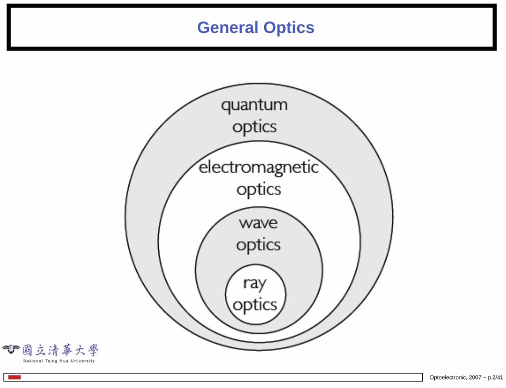
General Optics
Optoelectronic, 2007 – p.2/41
ElectroMagnetic waves
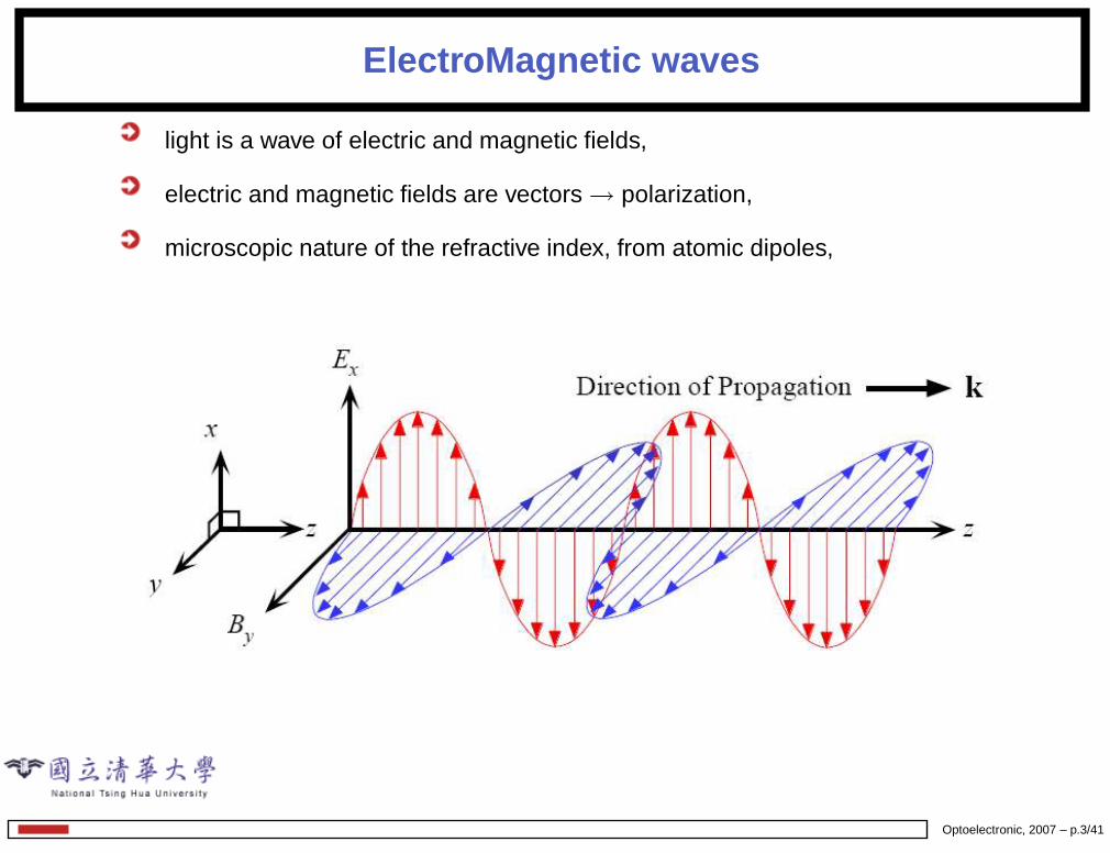
light is a wave of electric and magnetic fields,
electric and magnetic fields are vectors → polarization,
microscopic nature of the refractive index, from atomic dipoles,
Optoelectronic, 2007 – p.3/41
Syllabus
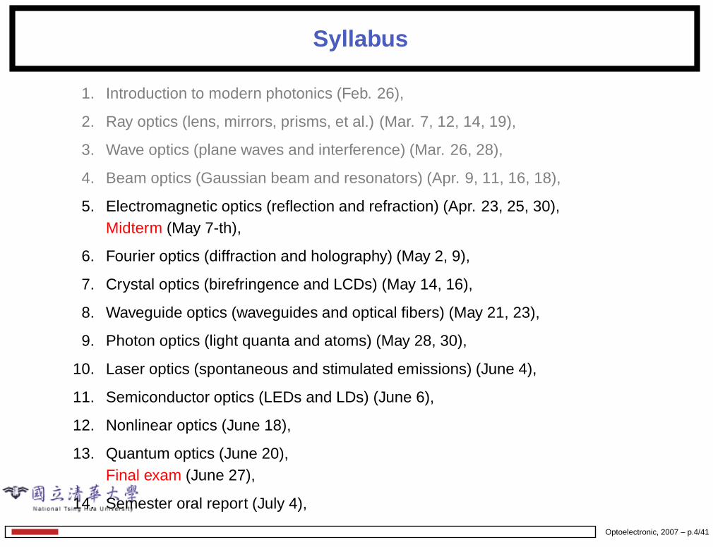
1. Introduction to modern photonics (Feb. 26),
2. Ray optics (lens, mirrors, prisms, et al.) (Mar. 7, 12, 14, 19),
3. Wave optics (plane waves and interference) (Mar. 26, 28),
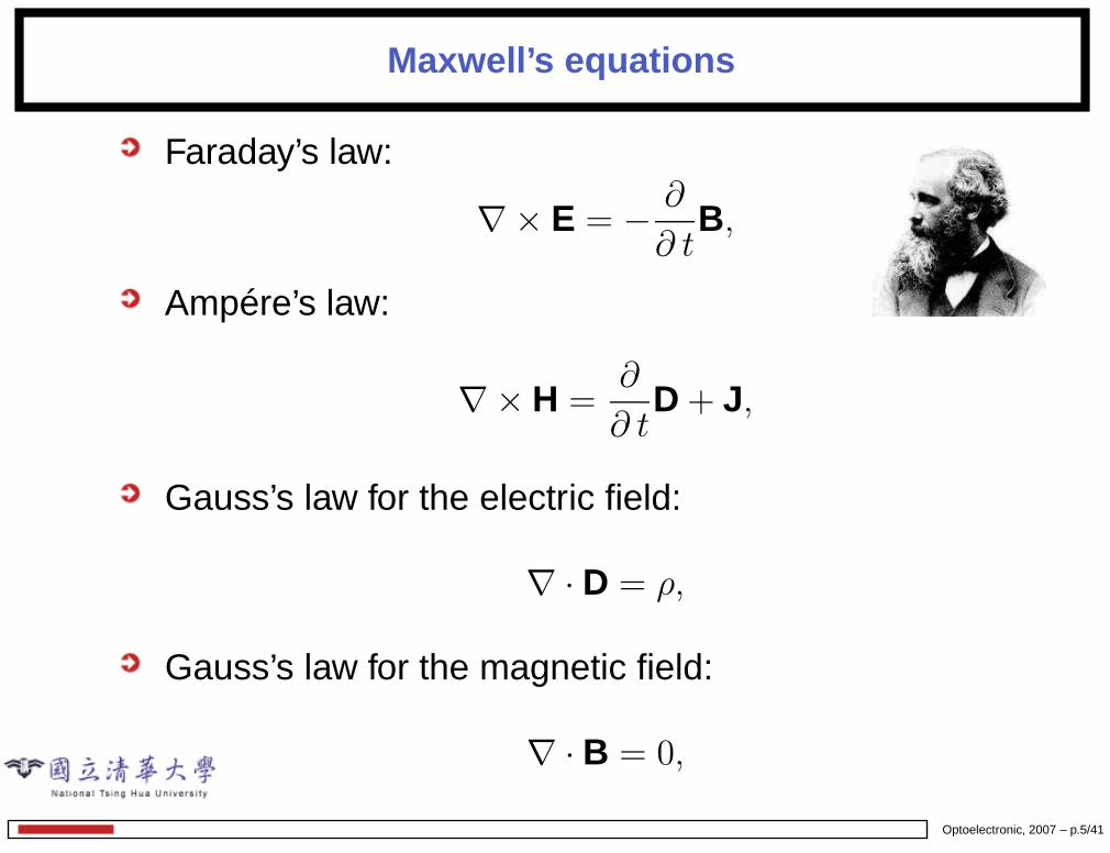
Maxwell’s equations in free space, there is vacuum, no free charges, no currents,J = ρ = 0,
both E and B satisfy wave equation,
∇2E = ǫ0µ0∂2E∂t2
,
we can use the solutions of wave optics,
E(r, t) = E0exp(iωt)exp(−ik · r),
B(r, t) = B0exp(iωt)exp(−ik · r),
Optoelectronic, 2007 – p.6/41
Elementary electromagnetic waves
The k, B0, and E0 are standing perpendicular on each other,
k × B = − ω
c2E, k × E = ωB,
|B0| = |E0|/c,
light is a TEM wave,
Optoelectronic, 2007 – p.7/41
Poynting’s theorem
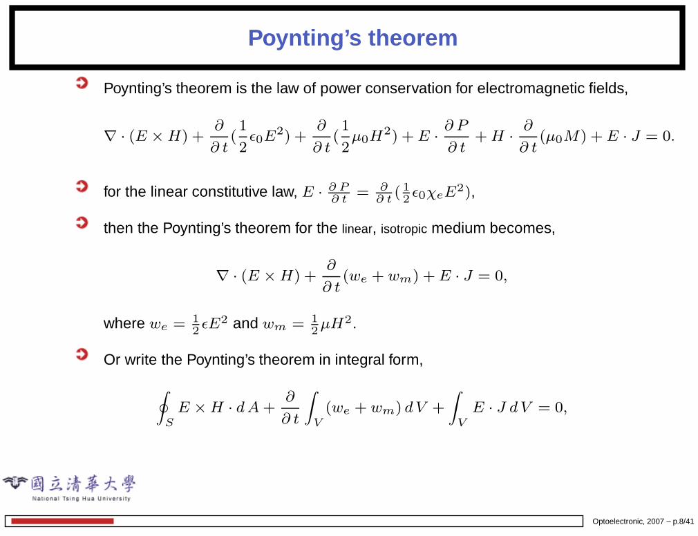
Poynting’s theorem is the law of power conservation for electromagnetic fields,
∇ · (E × H) +∂
∂ t(1
2ǫ0E2) +
∂
∂ t(1
2µ0H2) + E · ∂ P
∂ t+ H · ∂
∂ t(µ0M) + E · J = 0.
for the linear constitutive law, E · ∂ P∂ t
= ∂∂ t
( 12ǫ0χeE2),
then the Poynting’s theorem for the linear, isotropic medium becomes,
∇ · (E × H) +∂
∂ t(we + wm) + E · J = 0,
where we = 12ǫE2 and wm = 1
2µH2.
Or write the Poynting’s theorem in integral form,
∮
SE × H · d A +
∂
∂ t
∫
V(we + wm) d V +
∫
VE · J d V = 0,
Optoelectronic, 2007 – p.8/41
Energy density and intensity of a plane wave
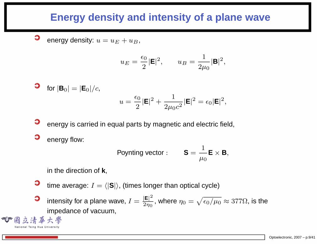
energy density: u = uE + uB ,
uE =ǫ0
2|E|2, uB =
1
2µ0|B|2,
for |B0| = |E0|/c,
u =ǫ0
2|E|2 +
1
2µ0c2|E|2 = ǫ0|E|2,
energy is carried in equal parts by magnetic and electric field,
energy flow:
Poynting vector : S =1
µ0E × B,
in the direction of k,
time average: I = 〈|S|〉, (times longer than optical cycle)
intensity for a plane wave, I =|E|2
2η0, where η0 =
√
ǫ0/µ0 ≈ 377Ω, is theimpedance of vacuum,
Optoelectronic, 2007 – p.9/41
Maxwell’s equations in a medium
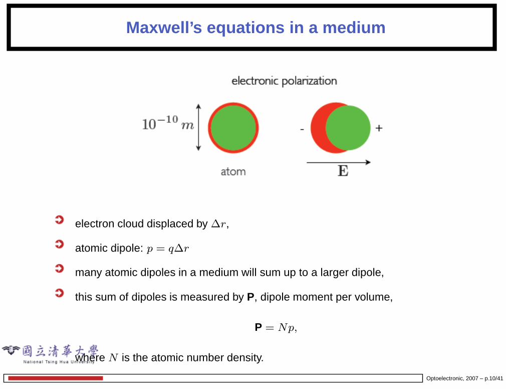
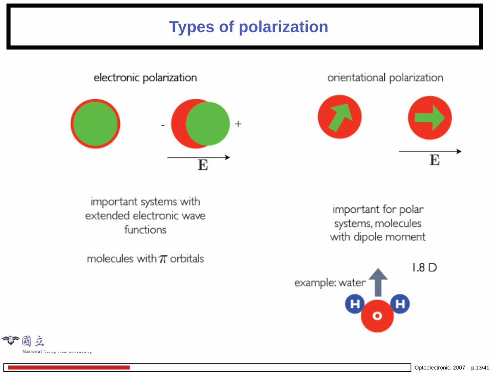
electron cloud displaced by ∆r,
atomic dipole: p = q∆r
many atomic dipoles in a medium will sum up to a larger dipole,
this sum of dipoles is measured by P, dipole moment per volume,
P = Np,
where N is the atomic number density.
Optoelectronic, 2007 – p.10/41
Maxwell’s equations in a medium
Total electron charges Q,
Q = −∮
P dA,
= −∫ ∫ ∫
∇ · P dV, Gauss theorem,
=
∫ ∫ ∫
ρ dV,
ρ = −∇ · P,
time dependent polarization creates also current,
J = Nqv,
= Nqdrdt
,
= Ndp
dt,
=dPdt
,
Optoelectronic, 2007 – p.11/41
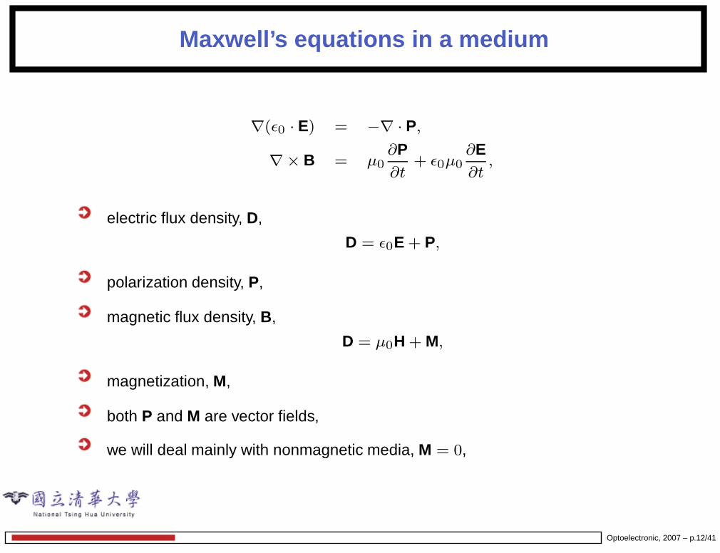
Maxwell’s equations in a medium
∇(ǫ0 · E) = −∇ · P,
∇× B = µ0∂P∂t
+ ǫ0µ0∂E∂t
,
electric flux density, D,
D = ǫ0E + P,
polarization density, P,
magnetic flux density, B,
D = µ0H + M,
magnetization, M,
both P and M are vector fields,
we will deal mainly with nonmagnetic media, M = 0,
Optoelectronic, 2007 – p.12/41
Types of polarization
Optoelectronic, 2007 – p.13/41
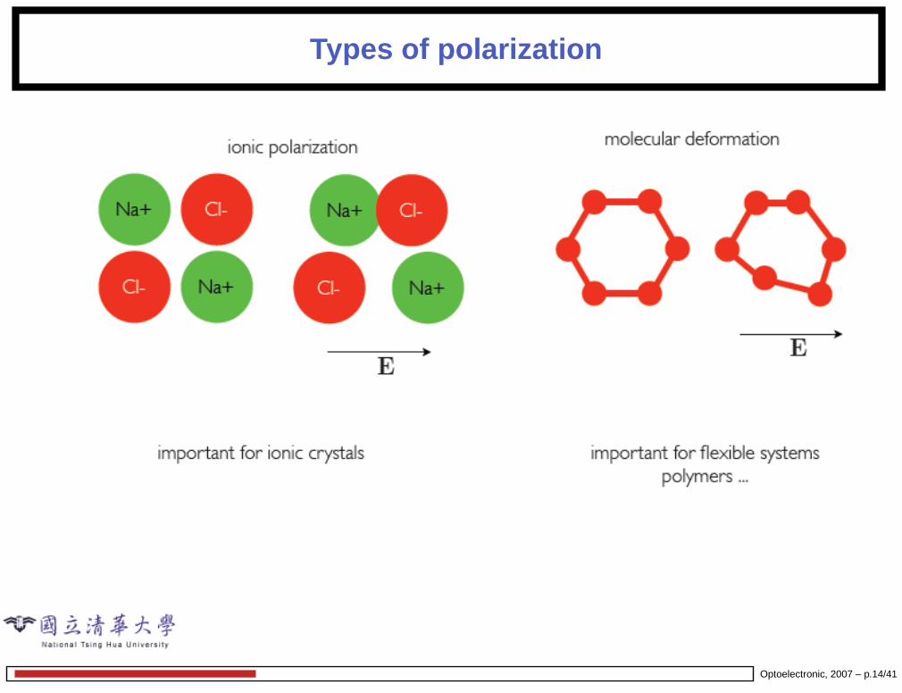
Types of polarization
Optoelectronic, 2007 – p.14/41
Dielectric media
linear: a medium is said to be linear if P(r, t) is linearly related to E(r, t), this isimportant for superposition (no superposition possible in a nonlinear medium),
nondispersive a medium is said to be nondispersive if
P(t) = E(t),
medium responds instantaneously (idealization, since polarization is never reallyinstantaneous),
homogeneous: a medium is said to be homogeneous if the relation between P andE are not a function of r,
isotropic: a medium is said to be isotropic if the relation between P and E are not afunction of direction P||E, example for anisotropy: birefringence,
Optoelectronic, 2007 – p.15/41
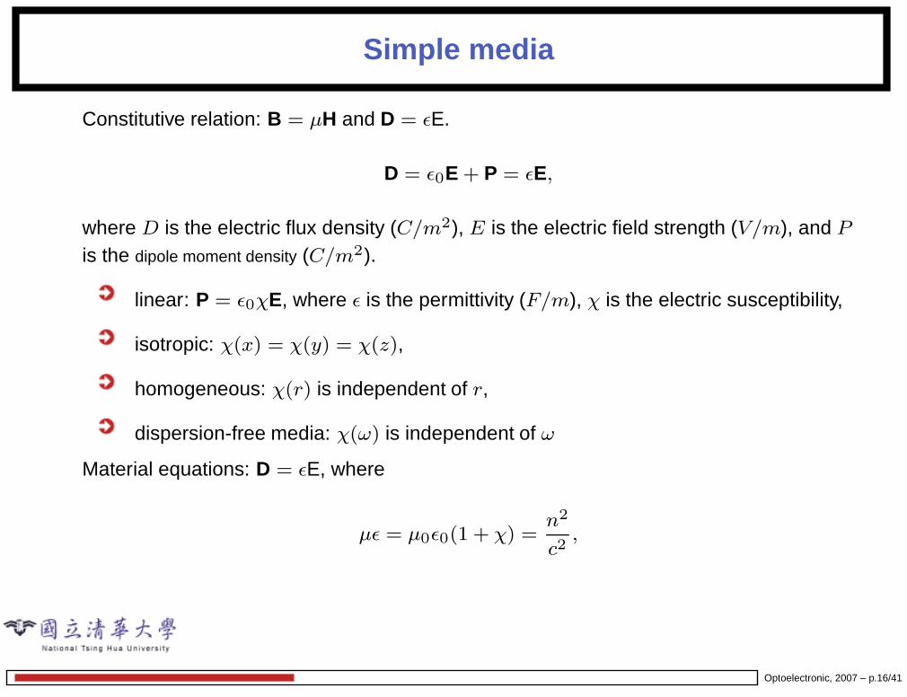
Simple media
Constitutive relation: B = µH and D = ǫE.
D = ǫ0E + P = ǫE,
where D is the electric flux density (C/m2), E is the electric field strength (V/m), and P
is the dipole moment density (C/m2).
linear: P = ǫ0χE, where ǫ is the permittivity (F/m), χ is the electric susceptibility,
isotropic: χ(x) = χ(y) = χ(z),
homogeneous: χ(r) is independent of r,
dispersion-free media: χ(ω) is independent of ω
Material equations: D = ǫE, where
µǫ = µ0ǫ0(1 + χ) =n2
c2,
Optoelectronic, 2007 – p.16/41
Model for the polarization response
damped harmonic oscillator
d2x
dt2+ σ
dx
dt+ ω2
0x =q
mE(t),
assume E(t) = E0exp(−iωt), and x(t) = x0exp(−iωt), then
x(t) =1
ω20 − iωσ − ω2
q
mE(t),
electronic dipole, p(t) = qx(t), and the polarization, P(t) = Nq∆x(t) = ǫ0χE(t),where χ is a complex number,
real media have usually multiple resonances,
Optoelectronic, 2007 – p.17/41
More general
χ(ω) =Nq2
ǫ0m
1
ω20 − iωσ − ω2
Quantum mechanics,
χ(ω) =Ne2
ǫ0m
∑
j
fj
ω2j − iωσj − ω2
where fj is the oscillator strength,
redefine,
χ(ν) = χ0ν20
ν20 − ν2 + iν∆ν
χ = χ′ + iχ”, where
χ′(ν) = χ0ν20(ν2
0 − ν2)
(ν20 − ν2)2 + (ν∆ν)2
,
χ”(ν) = χ0ν20ν∆ν
(ν20 − ν2)2 + (ν∆ν)2
, Lorentzian function,
Optoelectronic, 2007 – p.18/41
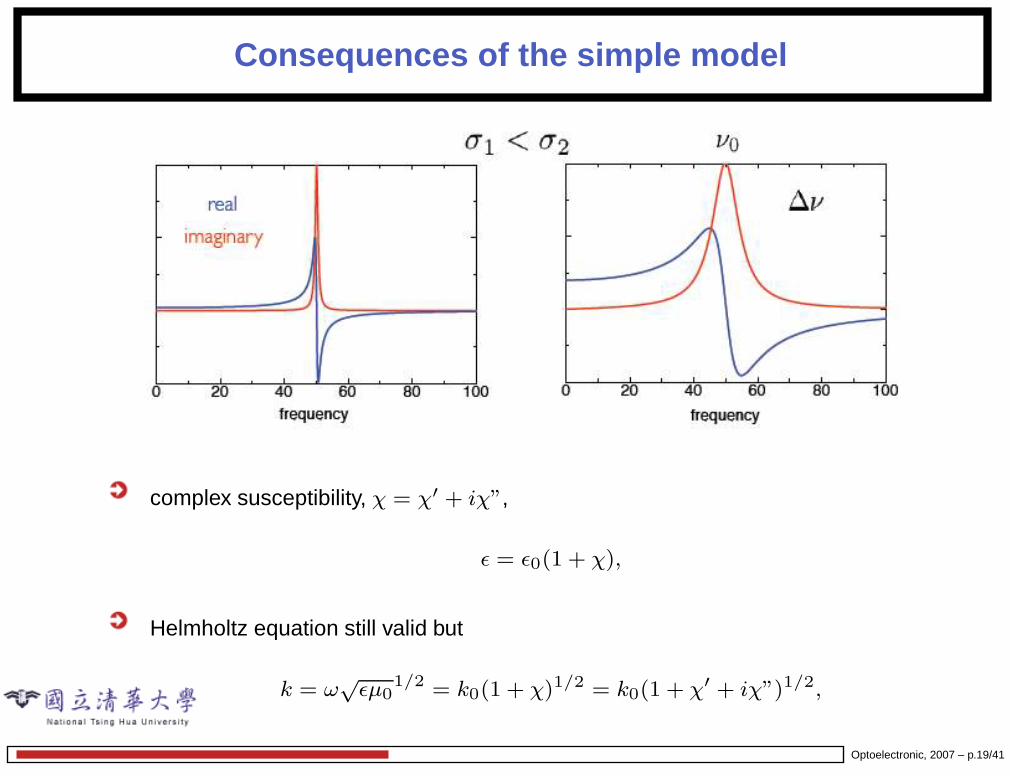
Consequences of the simple model
complex susceptibility, χ = χ′ + iχ”,
ǫ = ǫ0(1 + χ),
Helmholtz equation still valid but
k = ω√
ǫµ01/2 = k0(1 + χ)1/2 = k0(1 + χ′ + iχ”)1/2,
Optoelectronic, 2007 – p.19/41
Relation to refractive index
plane waves: exp(−ikz),
k = ω√
ǫµ01/2 = k0(1 + χ)1/2 = k0(1 + χ′ + iχ”)1/2,
simplify
k = β − iα
2= n
ω
c,
refractive index is now also a complex number,
plane waves,
exp(−ikz) = exp(−iβz)exp(−α
2),
intensity,
I ∝ |exp(−ikz)|2 = exp(−αz),
where α is absorption coefficient,
Optoelectronic, 2007 – p.20/41
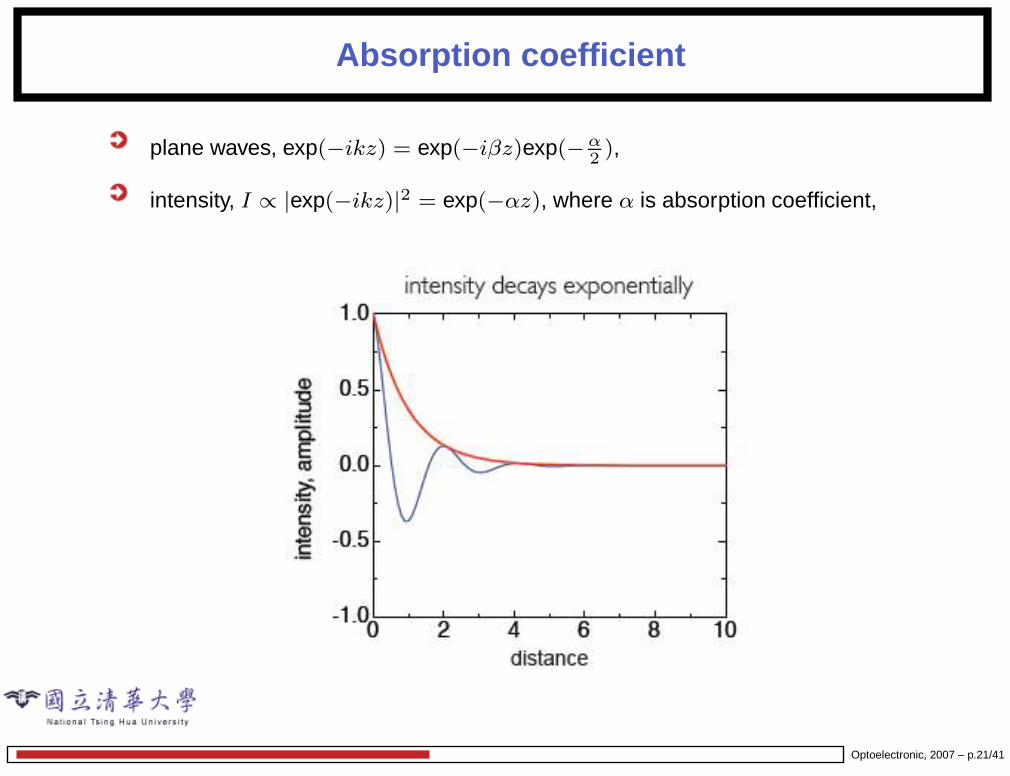
Absorption coefficient
plane waves, exp(−ikz) = exp(−iβz)exp(−α2),
intensity, I ∝ |exp(−ikz)|2 = exp(−αz), where α is absorption coefficient,
Optoelectronic, 2007 – p.21/41
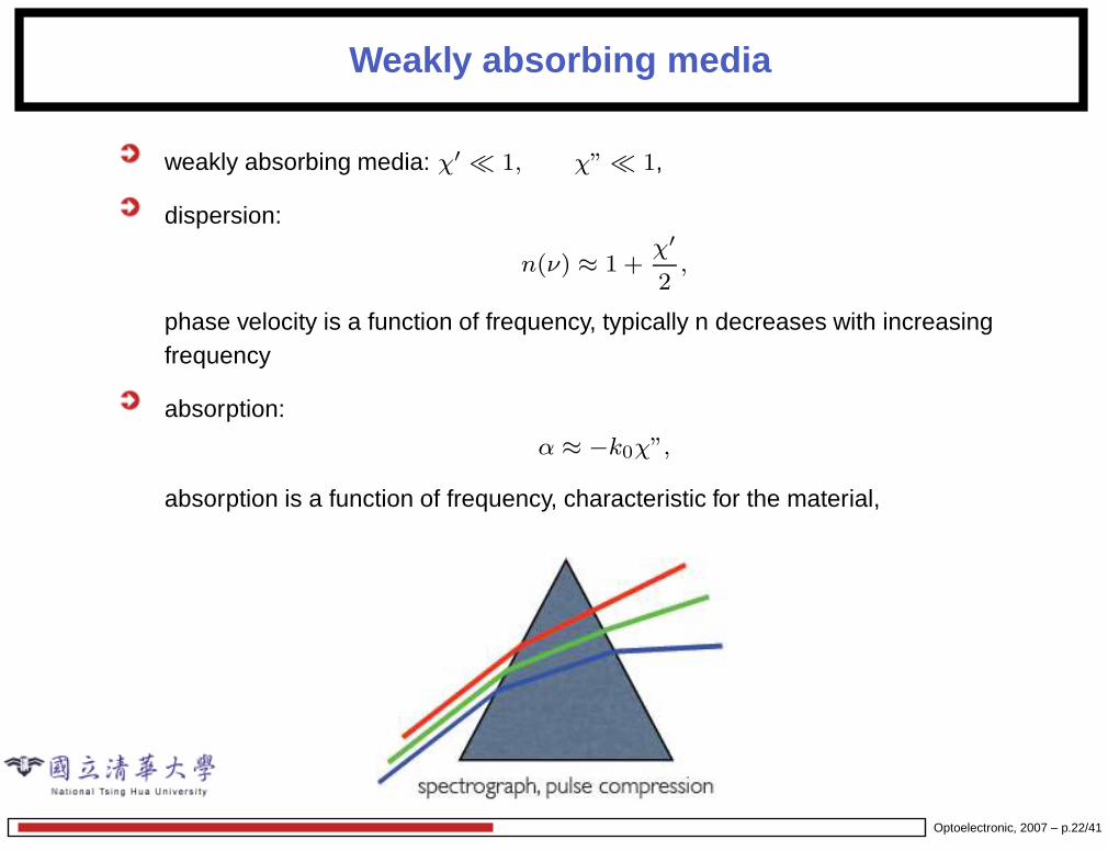
Weakly absorbing media
weakly absorbing media: χ′ ≪ 1, χ” ≪ 1,
dispersion:
n(ν) ≈ 1 +χ′
2,
phase velocity is a function of frequency, typically n decreases with increasingfrequency
absorption:
α ≈ −k0χ”,
absorption is a function of frequency, characteristic for the material,
Optoelectronic, 2007 – p.22/41
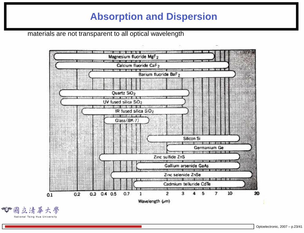
Absorption and Dispersion
materials are not transparent to all optical wavelength
Optoelectronic, 2007 – p.23/41
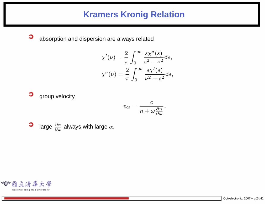
Kramers Kronig Relation
absorption and dispersion are always related
χ′(ν) =2
π
∫ ∞
0
sχ”(s)
s2 − ν2ds,
χ”(ν) =2
π
∫ ∞
0
sχ′(s)
ν2 − s2ds,
group velocity,
vG =c
n + ω ∂n∂ω
,
large ∂n∂ω
always with large α,
Optoelectronic, 2007 – p.24/41
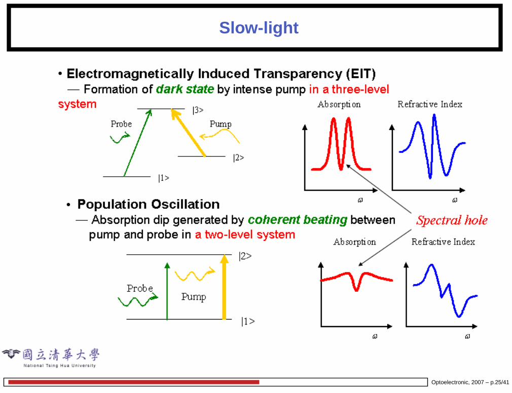
Slow-light
Optoelectronic, 2007 – p.25/41
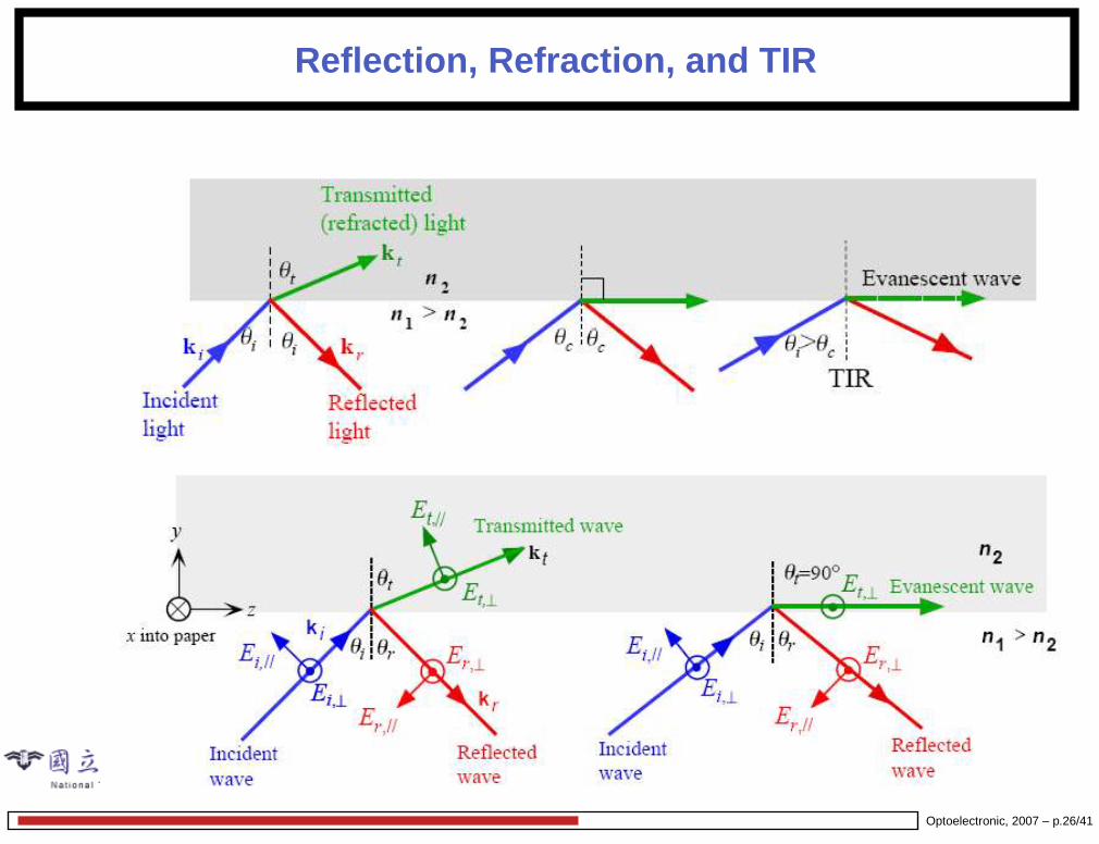
Reflection, Refraction, and TIR
Optoelectronic, 2007 – p.26/41
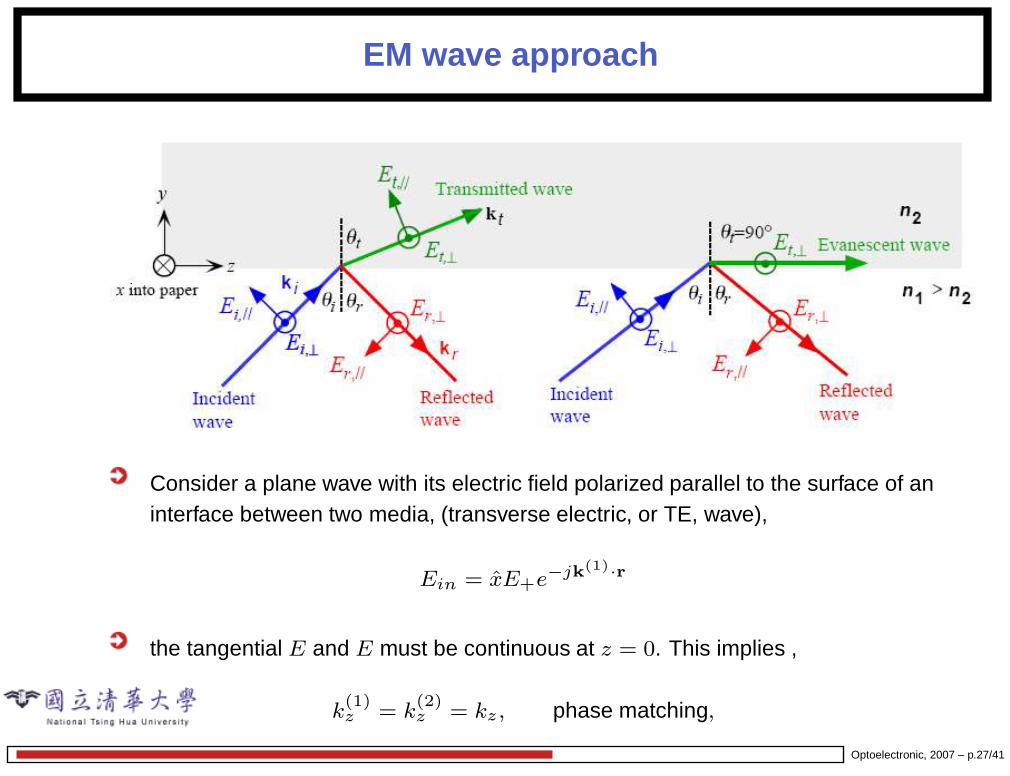
EM wave approach
Consider a plane wave with its electric field polarized parallel to the surface of aninterface between two media, (transverse electric, or TE, wave),
Ein = xE+e−jk(1)·r
the tangential E and E must be continuous at z = 0. This implies ,
k(1)z = k
(2)z = kz , phase matching,
Optoelectronic, 2007 – p.27/41
EM wave approach
The consequence is Snell’s law,
√µ1ǫ1 sin θ1 =
√µ2ǫ2 sin θ2.
At y < 0, the superposition of the incident and reflected waves is,
Ex = [E(1)+ e−jk
(1)y y + E
(1)− e+jk
(1)y y ]e−jkzz ,
from Faraday’s law,
Hz = − k(1)y
ωµ1[E
(1)+ e−jk
(1)y y − E
(1)− e+jk
(1)y y ]e−jkzz ,
where
k(1)y
ωµ1=
√
ǫ1
µ1cos θ1 ≡ Y
(1)0 ,
is the characteristic admittance by medium 1 to a TE wave at inclination θ1 with respect
at the y direction. The inverse of Y(1)0 is the characteristic impedance Z
(1)0 .
Optoelectronic, 2007 – p.28/41
EM wave approach
At y > 0, the transmitted waves is,
Ex = E(2)+ e−jk
(2)y ye−jkzz ,
with the z component of the H field,
Hz = − k(2)y
ωµ2E
(2)+ e−jk
(2)y ye−jkzz ,
with the characteristic admittance in medium 2,
k(2)y
ωµ2=
√
ǫ2
µ2cos θ2 ≡ Y
(2)0 .
Continuity of the tangential components of E and H requires the ratio
Z ≡ −Ex
Hz
to be continuous. Z is the wave impedance at the interface.
Optoelectronic, 2007 – p.29/41
EM wave approach
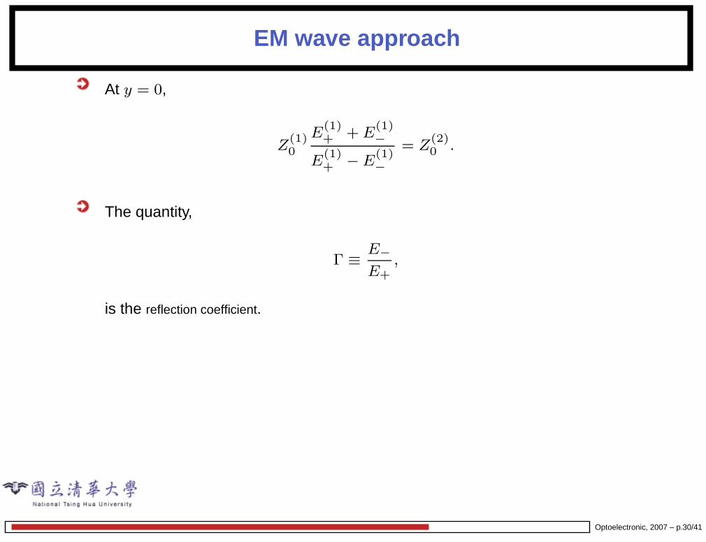
At y = 0,
Z(1)0
E(1)+ + E
(1)−
E(1)+ − E
(1)−
= Z(2)0 .
The quantity,
Γ ≡ E−
E+,
is the reflection coefficient.
Optoelectronic, 2007 – p.30/41
EM wave approach
For E(1)− /E
(1)+ ,
Γ(1) =Z
(2)0 − Z
(1)0
Z(2)0 + Z
(1)0
,
using Snell’s law,
Γ(1) =
√
1 − sin2 θ1 −√
1 − sin2 θ1ǫ1µ1ǫ2µ2
√
ǫ2µ1ǫ1µ2
√
1 − sin2 θ1 +√
1 − sin2 θ1ǫ1µ1ǫ2µ2
√
ǫ2µ1ǫ1µ2
.
The density of power flow in the y direction is
1
2Re[E × H∗] · y = −1
2Re[ExHz ] =
1
2Y
(1)0 |E(1)
+ |2(1 − |Γ(1)|2).
Thus |Γ|2 is the ratio of reflected to incident power flow.
Optoelectronic, 2007 – p.31/41
Fresnel’s equations: TE
for TE waves, E⊥, the reflection coefficient,
r⊥ =E
(1)− (0)
E(1)+ (0)
=
√
1 − sin2 θ1 −√
1 − sin2 θ1ǫ1µ1ǫ2µ2
√
ǫ2µ1ǫ1µ2
√
1 − sin2 θ1 +√
1 − sin2 θ1ǫ1µ1ǫ2µ2
√
ǫ2µ1ǫ1µ2
,
=cos θ1 − [n2 − sin2 θ1]1/2
cos θ1 + [n2 − sin2 θ1]1/2,
where n ≡ n2n1
= ( ǫ2ǫ1
)1/2, and the transmission coefficients,
t⊥ =2 cos θ1
cos θ1 + [n2 − sin2 θ1]1/2,
relations between reflection and transmission coefficients,
r⊥ + 1 = t⊥,
Optoelectronic, 2007 – p.32/41
Fresnel’s equations: TM
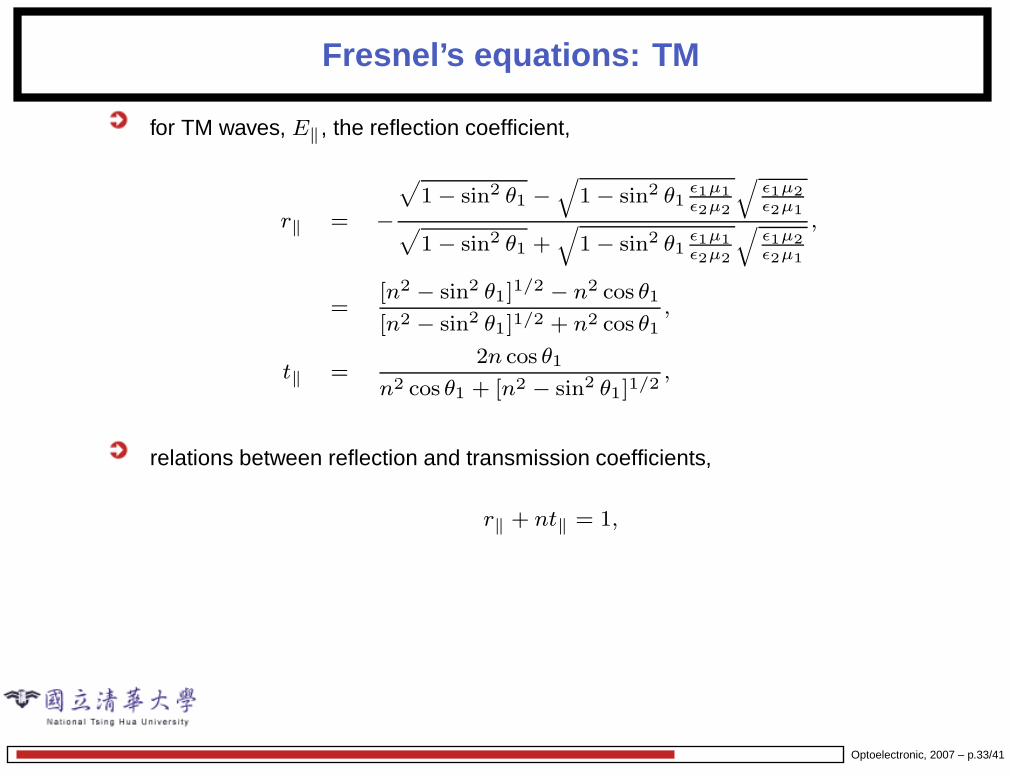
for TM waves, E‖, the reflection coefficient,
r‖ = −
√
1 − sin2 θ1 −√
1 − sin2 θ1ǫ1µ1ǫ2µ2
√
ǫ1µ2ǫ2µ1
√
1 − sin2 θ1 +√
1 − sin2 θ1ǫ1µ1ǫ2µ2
√
ǫ1µ2ǫ2µ1
,
=[n2 − sin2 θ1]1/2 − n2 cos θ1
[n2 − sin2 θ1]1/2 + n2 cos θ1,
t‖ =2n cos θ1
n2 cos θ1 + [n2 − sin2 θ1]1/2,
relations between reflection and transmission coefficients,
r‖ + nt‖ = 1,
Optoelectronic, 2007 – p.33/41
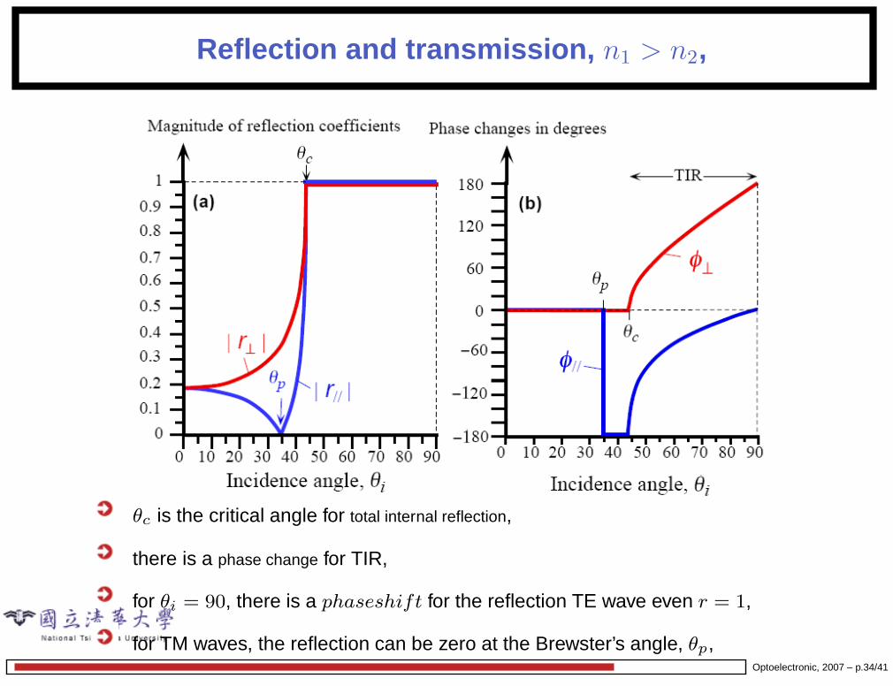
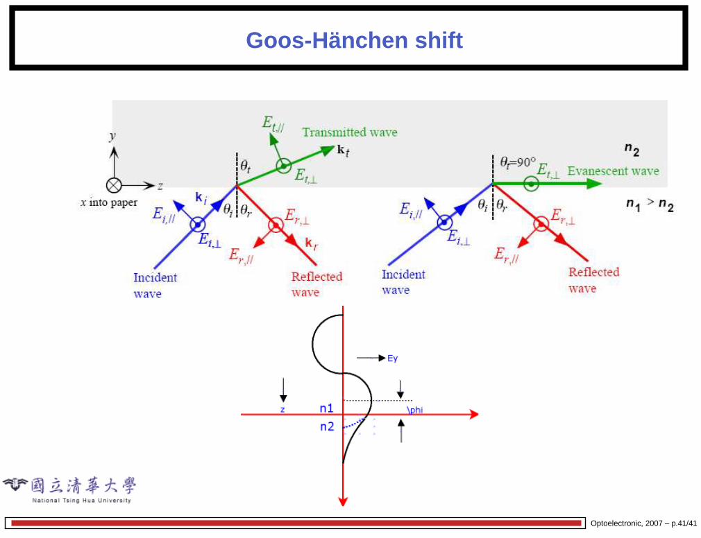
Reflection and transmission, n1 > n2,
θc is the critical angle for total internal reflection,
there is a phase change for TIR,
for θi = 90, there is a phaseshift for the reflection TE wave even r = 1,
for TM waves, the reflection can be zero at the Brewster’s angle, θp,Optoelectronic, 2007 – p.34/41
EM wave approach: TM
Consider a plane wave with its magnetic field polarized parallel to the surface of aninterface between two media, (transverse magnetic, or TM, wave),
at y < 0, the superposition of the incident and reflected waves is,
Hx = [H(1)+ e−jk
(1)y y + H
(1)− e+jk
(1)y y]e−jkzz ,
from Ampére’s law,
Ez =k(1)y
ωǫ1[H
(1)+ e−jk
(1)y z − H
(1)− e+jk
(1)y z ]e−jkzz .
At y > 0, the transmitted waves is,
Hx = H(2)+ e−jk
(2)y ye−jkzz ,
with the z component of the E field,
Ez =k(2)y
ωǫ2H
(2)+ e−jk
(2)y ye−jkzz ,
Optoelectronic, 2007 – p.35/41
EM wave approach: TM
with the characteristic admittance of the traveling TM wave,
Y0 =ωǫ
ky=
√
ǫ
µ
1
cos θ.
continuity of the tangential components of E and H requires the ratio
Z ≡ Ez
Hx
to be continuous. Z is the wave impedance at the interface.
at y = 0,
Z(1)0
H(1)+ − H
(1)−
H(1)+ + H
(1)−
= Z(2)0 .
The quantity, Γ ≡ −H−
H+, is the reflection coefficient.
Optoelectronic, 2007 – p.36/41
EM wave approach: TM
For E(1)− /E
(1)+ ,
Γ(1) =Z
(2)0 − Z
(1)0
Z(2)0 + Z
(1)0
,
using Snell’s law,
Γ(1) = −
√
1 − sin2 θ1 −√
1 − sin2 θ1ǫ1µ1ǫ2µ2
√
ǫ1µ2ǫ2µ1
√
1 − sin2 θ1 +√
1 − sin2 θ1ǫ1µ1ǫ2µ2
√
ǫ1µ2ǫ2µ1
,
=[n2 − sin2 θ1]1/2 − n2 cos θ1
[n2 − sin2 θ1]1/2 + n2 cos θ1,
t‖ =2n cos θ1
n2 cos θ1 + [n2 − sin2 θ1]1/2,
TM waves can be transmitted reflection-free at a dielectric interface, whenµ1 = µ2 = µ0, for the angle θ1 = θB , the so-called Brewster angle,
θB = tan−1
√
ǫ2
ǫ1.
Optoelectronic, 2007 – p.37/41
Total internal reflection
If medium 1 has a larger value of√
µǫ, optical denser, than medium 2, Snell’s lawfails to yield a real angle θ2 for a certain range of angle of incidence.
for µ1 = µ2 = µ0,
sin θc =
√
ǫ2
ǫ1=
n2
n1.
When no real solution of θ2 are found, the propagation constant must be allowedto become negative imaginary,
k(2)z = k
(1)z , k
(2)y = −jα
(2)y .
In this case,
[k(2)z ]2 + [k
(2)y ]2 = [k
(2)z ]2 − [α
(2)y ]2 = ω2µ0ǫ2,
and
k(2)z =
√
ω2µ0ǫ2 + [α(2)z ]2.
Optoelectronic, 2007 – p.38/41
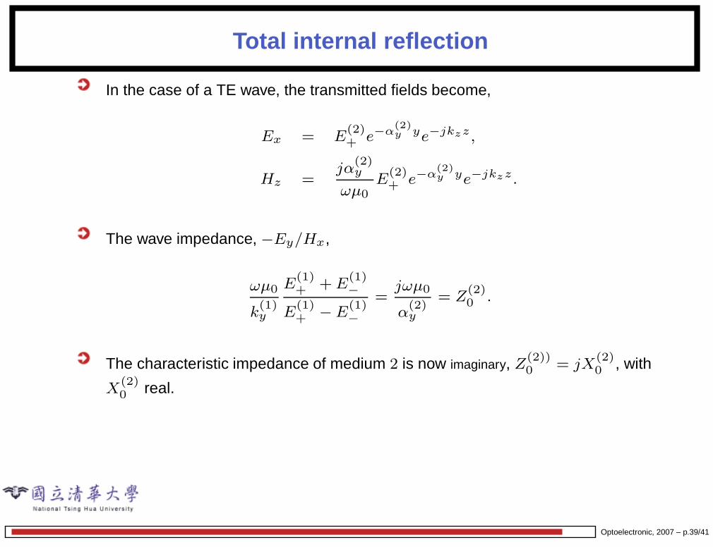
Total internal reflection
In the case of a TE wave, the transmitted fields become,
Ex = E(2)+ e−α
(2)y ye−jkzz ,
Hz =jα
(2)y
ωµ0E
(2)+ e−α
(2)y ye−jkzz .
The wave impedance, −Ey/Hx,
ωµ0
k(1)y
E(1)+ + E
(1)−
E(1)+ − E
(1)−
=jωµ0
α(2)y
= Z(2)0 .
The characteristic impedance of medium 2 is now imaginary, Z(2))0 = jX
(2)0 , with
X(2)0 real.
Optoelectronic, 2007 – p.39/41
Total internal reflection
Then the reflection coefficient, Γ = E(1)− /E
(1)+ ,
Γ(1) =E
(1)−
E(1)+
=jX
(2)0 − Z
(1)0
jX(2)0 + Z
(1)0
,
|Γ(1)| = 1, and the magnitude of the reflected wave, E(1)− , equals to the magnitude