ORNL/TM-2016/693 Supervisory Control System for Multi- Modular Advanced Reactors Sacit M. Cetiner (ORNL) Michael D. Muhlheim (ORNL) Askin Guler-Yigitoglu (ORNL) Randall J. Belles (ORNL) Scott M. Greenwood (ORNL) T. Jay Harrison (ORNL) Richard S. Denning (OSU emeritus) Christopher A. Bonebrake (PNNL) Gerges Dib (PNNL) David Grabaskas (ANL) Acacia J. Brunett (ANL) November 2016 Approved for public release. Distribution is unlimited
Transcript
ORNL/TM-2016/693
Supervisory Control System for Multi-Modular Advanced Reactors
Sacit M. Cetiner (ORNL) Michael D. Muhlheim (ORNL) Askin Guler-Yigitoglu (ORNL)
Randall J. Belles (ORNL) Scott M. Greenwood (ORNL)
T. Jay Harrison (ORNL)
Richard S. Denning (OSU emeritus)
Christopher A. Bonebrake (PNNL) Gerges Dib (PNNL)
David Grabaskas (ANL) Acacia J. Brunett (ANL)
November 2016
Approved for public release. Distribution is unlimited
DOCUMENT AVAILABILITY
Reports produced after January 1, 1996, are generally available free via US Department of Energy (DOE) SciTech Connect. Website http://www.osti.gov/scitech/ Reports produced before January 1, 1996, may be purchased by members of the public from the following source: National Technical Information Service 5285 Port Royal Road Springfield, VA 22161 Telephone 703-605-6000 (1-800-553-6847) TDD 703-487-4639 Fax 703-605-6900 E-mail [email protected] Website http://www.ntis.gov/help/ordermethods.aspx Reports are available to DOE employees, DOE contractors, Energy Technology Data Exchange representatives, and International Nuclear Information System representatives from the following source: Office of Scientific and Technical Information PO Box 62 Oak Ridge, TN 37831 Telephone 865-576-8401 Fax 865-576-5728 E-mail [email protected] Website http://www.osti.gov/contact.html
This report was prepared as an account of work sponsored by an agency of the United States Government. Neither the United States Government nor any agency thereof, nor any of their employees, makes any warranty, express or implied, or assumes any legal liability or responsibility for the accuracy, completeness, or usefulness of any information, apparatus, product, or process disclosed, or represents that its use would not infringe privately owned rights. Reference herein to any specific commercial product, process, or service by trade name, trademark, manufacturer, or otherwise, does not necessarily constitute or imply its endorsement, recommendation, or favoring by the United States Government or any agency thereof. The views and opinions of authors expressed herein do not necessarily state or reflect those of the United States Government or any agency thereof.
ORNL/TM-2016/693
Reactor and Nuclear Systems Division
SUPERVISORY CONTROL SYSTEM FOR MULTI-MODULAR ADVANCED REACTORS
Sacit M. Cetiner (ORNL) Michael D. Muhlheim (ORNL) Askin Guler-Yigitoglu (ORNL)
Randall J. Belles (ORNL) Scott M. Greenwood (ORNL)
T. Jay Harrison (ORNL)
Richard S. Denning (OSU emeritus)
Christopher A. Bonebrake (PNNL) Gerges Dib (PNNL)
David Grabaskas (ANL) Acacia J. Brunett (ANL)
Date Published: November 30, 2016
Prepared by OAK RIDGE NATIONAL LABORATORY
Oak Ridge, TN 37831-6283 managed by
UT-BATTELLE, LLC for the
US DEPARTMENT OF ENERGY under contract DE-AC05-00OR22725
iii
CONTENTS
LIST OF FIGURES ............................................................................................................................ vii LIST OF TABLES ............................................................................................................................... xi ACRONYMS ..................................................................................................................................... xiii ACKNOWLEDGMENTS .................................................................................................................. xv EXECUTIVE SUMMARY .............................................................................................................. xvii ABSTRACT ...................................................................................................................................... xxi 1. INTRODUCTION ........................................................................................................................ 1 2. DEVELOPMENT OF A RISK-INFORMED SUPERVISORY CONTROL SYSTEM .............. 3 2.1 FUNCTION OF A CONTROL SYSTEM .................................................................................. 4 2.2 CONSTRAINTS ON CONTROL SYSTEMS ............................................................................ 5 2.3 REQUIREMENTS AND CAPABILITIES OF THE SCS ......................................................... 6
2.3.1 Supervisory control system hierarchy ............................................................................ 6 2.3.2 System-level functional taxonomy ................................................................................. 6 2.3.3 Human-machine interface .............................................................................................. 7
2.4 FUNCTIONAL ELEMENTS OF THE SCS ARCHITECTURE ............................................... 8 2.4.1 Probabilistic decision-making module ......................................................................... 10 2.4.2 Enhanced risk monitors module ................................................................................... 10 2.4.3 Performance-based decision-making module .............................................................. 11 2.4.4 Utility Theory Algorithm to Select a Control Option .................................................. 11
2.5 SOFTWARE IMPLEMENTATION OF THE SUPERVISORY CONTROL SYSTEM ......... 11 3. PROBABILISTIC DECISION-MAKING MODEL ................................................................. 13 3.1 CONTROL SYSTEM LOGIC MODELS ................................................................................ 14
3.1.1 Failure data ................................................................................................................... 17 3.2 IDENTIFICATION OF CONTROL OPTIONS ....................................................................... 18
3.2.1 Reconfiguration and execution of probabilistic models .............................................. 19 3.2.2 Reconstruction of ET from component failure .......................................................... 20 3.2.3 Deconstruction of ET to identify corrective actions ................................................. 21
3.3 INTERFACES TO ENHANCED RISK MONITORS (ERM) MODULE ............................... 24 3.4 RESULTS OF PROBABILISTIC MODELS ........................................................................... 26 4. PERFORMANCE-BASED SYSTEM MODEL ........................................................................ 29 4.1 REACTOR AND PRIMARY HEAT TRANSPORT SYSTEM ............................................... 29 4.2 INTERMEDIATE HEAT EXCHANGER AND INTERMEDIATE HEAT
TRANSPORT SYSTEM .......................................................................................................... 31 4.3 STEAM GENERATOR SYSTEM ........................................................................................... 33 4.4 POWER CONVERSION SYSTEM ......................................................................................... 35 4.5 CONTROL SYSTEMS ............................................................................................................. 39
4.5.1 Level control ................................................................................................................ 40 5. UTILITY THEORY ALGORITHM USED TO GENERATE A DECISION ......................... 43 5.1 LIKELIHOOD OF SUCCESS .................................................................................................. 44 5.2 UTILITY VARIABLES ........................................................................................................... 45 5.3 UTILITY WEIGHTS ................................................................................................................ 48 5.4 UTILITY FUNCTIONS ........................................................................................................... 48 6. DEMONSTRATION OF A SUPERVISORY CONTROL SYSTEM ....................................... 51 6.1 PROBABILISTICALLY IDENTIFIED CONTROL ACTIONS ............................................. 52 6.2 PERFORMANCED-BASED ASSESSMENT OF CONTROL OPTIONS .............................. 53
6.2.1 Control option 3 ........................................................................................................... 54 6.2.2 Control option 4 ........................................................................................................... 58
6.3 ASSESSMENT OF CONTROL OPTIONS USING UTILITY THEORY .............................. 62
iv
6.3.1 Assessment of control option 3 .................................................................................... 63 6.3.2 Assessment of control option 4 .................................................................................... 66
6.4 GENERATION OF CONTROL SIGNAL ............................................................................... 68 7. SUMMARY AND CONCLUSIONS ......................................................................................... 69 7.1 SUMMARY OF A RISK-INFORMED PERFORMANCE-BASED DECISION-
MAKING PROCESS ................................................................................................................ 69 7.2 TECHNICAL ACCOMPLISHMENTS .................................................................................... 70
7.2.1 Advancement in control system technology ................................................................ 70 7.2.2 Actual plant conditions evaluated in real-time............................................................. 70 7.2.3 Uncertainties in component behavior included ............................................................ 70 7.2.4 Dynamic behavior of models ....................................................................................... 71
7.3 IMPORTANCE OF A RISK-INFORMED PERFORMANCE-BASKED SCS ....................... 71 7.3.1 Reduction in control room operators ........................................................................... 71 7.3.2 Reduction in O&M costs ............................................................................................. 72 7.3.3 Optimization of design and performance ..................................................................... 72 7.3.4 Increased plant availability, reliability, and safety ....................................................... 72
7.4 OTHER APPLICATIONS ........................................................................................................ 73 7.5 FUTURE WORK ...................................................................................................................... 73 8. References .................................................................................................................................. 75 APPENDIX A—ALMR PRISM PLANT DESCRIPTION ............................................................. A-2 A-1 Overall Plant Description ........................................................................................................ A-2 A-2 Reactor Module ....................................................................................................................... A-3 A-3 Reactivity Control and Shutdown ........................................................................................... A-3 A-4 Intermediate Heat Transport System ....................................................................................... A-3 A-5 Steam Generator System ......................................................................................................... A-5 A-6 Power Conversion System ...................................................................................................... A-7 APPENDIX B—FAILURE MODES AND RELIABILITY DATA FOR PRISM BOP ................. B-1 B-1 Introduction ............................................................................................................................ B-1 B.2 Balance of Plant Reliability Data ........................................................................................... B-1 B-2.1 Turbines .................................................................................................................................. B-2
B-2.1.1 Failure modes ............................................................................................................. B-2 B-2.1.2 Reliability Data ........................................................................................................ B-3
D-3 Application of ERM Module in SCS ........................................................................................ D-4 D-4 References ................................................................................................................................ D-8
vii
LIST OF FIGURES
Fig. 2-1. Illustration of supervisory control execution. ................................................................................. 3 Fig. 2-2. Conceptual state space formed by arbitrary state variables x1 and x2. ........................................... 4 Fig. 2-3. Illustration of heat flow in a thermal power plant. ......................................................................... 6 Fig. 2-4. Functional architecture of the supervisory control system. ............................................................ 9 Fig. 2-5. Software elements of the supervisory control decision-making application. ............................... 12 Fig. 3-1. Secondary cooling system for the ALMR PRISM [5]. ................................................................ 14 Fig. 3-2. ET for steam flow to turbine with one steam generator in operation (Scenario 1). ..................... 16 Fig. 3-3. Sequence to identify probabilistically ranked control options. .................................................... 19 Fig. 3-4. TCV drifting-close status is communicated to the probabilistic model. ................................... 19 Fig. 3-5. FT reconstruction continues until ET branch link is identified. .................................................. 20 Fig. 3-6. ET branch numbers used to map FT to ET. ................................................................................. 20 Fig. 3-7. Reconfigured ET. ......................................................................................................................... 21 Fig. 3-8. Deconstruction of ET to identify decision options. ...................................................................... 22 Fig. 3-9. Deconstruction of ET branch 14 identifies SCS command signals for successfully
avoiding a trip setpoint. ................................................................................................................. 23 Fig. 3-10. FTs capture component failure and carry SCS control instructions (OOS). ............................. 24 Fig. 3-11. Interaction between the ERM module and the probabilistic decision-making module. ............. 24 Fig. 3-12. Probabilistic model updated based on ERM monitoring. ........................................................... 25 Fig. 3-13. Order of probabilistic options changes with degraded FW FCV. .............................................. 26 Fig. 4-1. Top-level diagram view of the ALMR PRISM power block. ...................................................... 29 Fig. 4-2. Reactor and primary heat transport system model for ALMR PRISM. ....................................... 30 Fig. 4-3. Diagram layer for the reactor kinetics and coolant subchannel. ................................................... 31 Fig. 4-4. Diagram view for the ALMR PRISM IHX. ................................................................................. 31 Fig. 4-5. Elements of the shell-side pressure drop. .................................................................................... 32 Fig. 4-6. Diagram view for the ALMR PRISM IHX shell-side flow paths. ............................................... 32 Fig. 4-7. ALMR PRISM intermediate heat transport system layout. .......................................................... 33 Fig. 4-8. Diagram layer for the ALMR PRISM steam generator and drum model. .................................. 34 Fig. 4-9. Illustration of key phenomena in the steam generator steam drum model. ................................. 35 Fig. 4-10. Drawing that shows the three main steam lines, the common header, the turbine stop
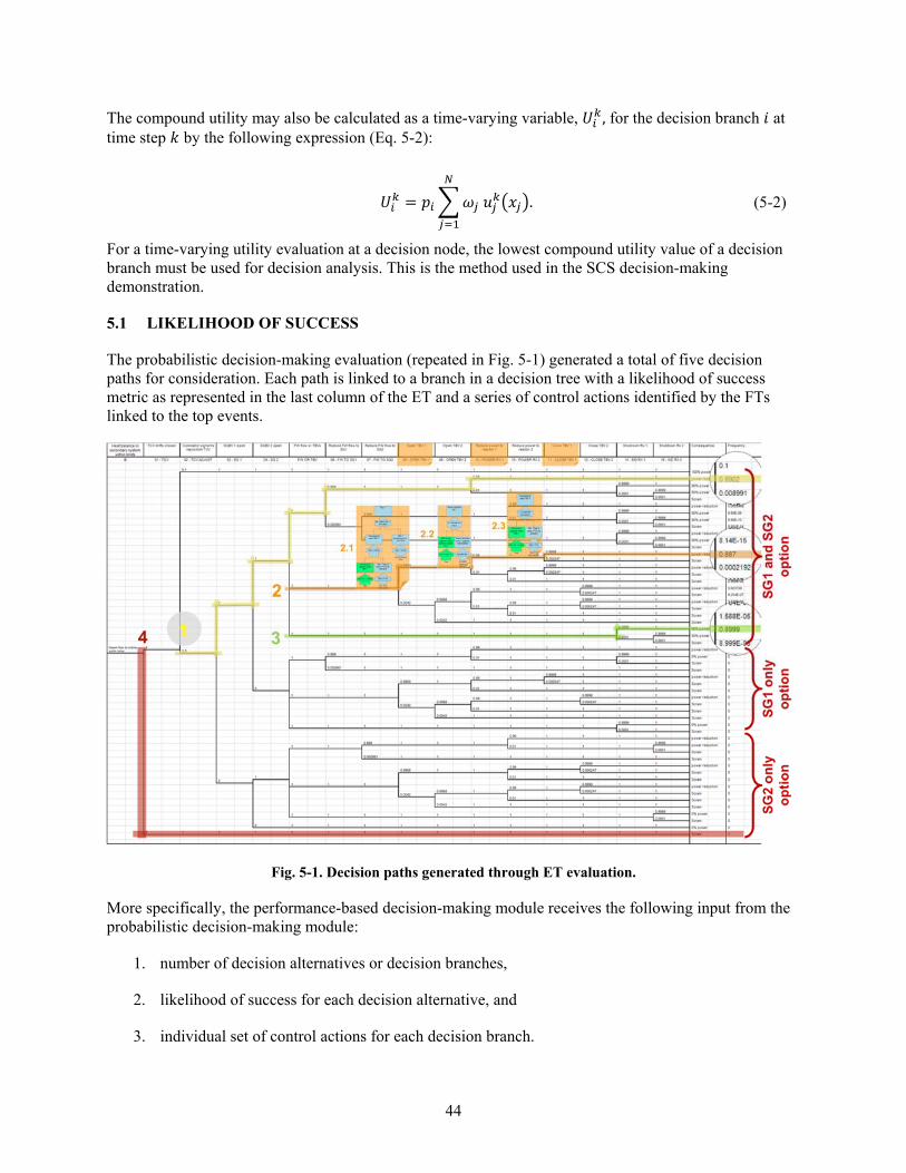
valve, and the turbine control valve. .............................................................................................. 36 Fig. 4-11. High-pressure FWH and connecting lines to steam generator drains. ....................................... 36 Fig. 4-12. ALMR PRISM power conversions system model layout. ......................................................... 37 Fig. 4-13. Typical nodalization example of a horizontal feedwater heater in RELAP5. ........................... 38 Fig. 4-14. Key phenomena in the deaerator model. .................................................................................... 38 Fig. 4-15. Temperature profiles of condensate and feedwater in a three-zone condenser. ........................ 39 Fig. 4-16. High-level sensing and actuation interfaces for the ALMR PRISM power block. .................... 40 Fig. 4-17. Level control system with feedback path only. .......................................................................... 40 Fig. 4-18. Level control system with feedforward and feedback paths. ..................................................... 41 Fig. 5-1. Decision paths generated through ET evaluation. ........................................................................ 44 Fig. 6-1. BOP components monitored by the ERM functions for SCS demonstration. .............................. 51 Fig. 6-2. Identification of control options based on probabilistic assessment. ........................................... 53 Fig. 6-3. (a) Turbine control valve opening as a function of time; (b) change of mass flow rate in
the BOP due to TCV closure. ........................................................................................................ 54 Fig. 6-4. Change of power output in response to partial closure of TCV followed by supervisory
control actions: (a) power block thermal output; (b) reactor modules 1 and 2 thermal outputs. ........................................................................................................................................... 55
Fig. 6-5. Change of generator electrical output in response to partial closure of TCV followed by supervisory control actions. ........................................................................................................... 55
viii
Fig. 6-6. Change of core inlet and mixed outlet temperatures in reactor modules 1 and 2 in response to partial closure of TCV followed by supervisory control actions. ............................... 56
Fig. 6-7. Change of primary cold pool temperatures in reactor modules 1 and 2 in response to partial closure of TCV followed by supervisory control actions. .................................................. 56
Fig. 6-8. Change of core exit temperatures in reactor modules 1 and 2 in response to partial closure of TCV followed by supervisory control actions: (a) exit temperatures in an average driver assembly; (b) exit temperatures in an average blanket assembly. .......................... 57
Fig. 6-9. Power conversion system steam header dynamics in response to partial closure of TCV followed by supervisory control actions: (a) change of pressure; (b) change of temperature. ................................................................................................................................... 57
Fig. 6-10. Change of liquid levels in three steam generator drums in response to partial closure of TCV followed by supervisory control actions. .............................................................................. 58
Fig. 6-11. Change of power output in response to partial closure of TCV followed by supervisory control actions: (a) power block thermal output; (b) reactor modules 1 and 2 thermal outputs. ........................................................................................................................................... 59
Fig. 6-12. Change of generator electrical output in response to partial closure of TCV followed by supervisory control actions. ...................................................................................................... 59
Fig. 6-13. Change of core inlet (a) and core mixed outlet (4) temperatures in reactor modules 1 and 2 in response to partial closure of TCV followed by supervisory control actions based on Scenario 4. ................................................................................................................................ 60
Fig. 6-14. Change of primary cold pool temperatures in reactor modules 1 and 2 in response to partial closure of TCV followed by supervisory control actions based on Scenario 4. ................. 60
Fig. 6-15. Change of core exit temperatures in reactor modules 1 and 2 in response to partial closure of TCV followed by supervisory control actions based on Scenario 4: (a) exit temperatures in an average driver assembly; (b) exit temperatures in an average blanket assembly. ........................................................................................................................................ 61
Fig. 6-16. Power conversion system steam header dynamics in response to partial closure of TCV followed by supervisory control actions based on Scenario 4: (a) change of pressure; (b) change of temperature. ................................................................................................................... 61
Fig. 6-17. Change of liquid levels in three steam generator drums in response to partial closure of TCV followed by supervisory control actions based on Scenario 4. ............................................. 62
Fig. 6-18. Variation of utility for the driver assembly exit temperature attribute. ...................................... 64 Fig. 6-19. Variation of utility for the primary system cold pool temperature attribute. ............................. 64 Fig. 6-20. Variation of utility for the header pressure attribute. ................................................................. 65 Fig. 6-21. Variation of utility for the steam generator drum liquid level attribute. .................................... 65 Fig. 6-22. Variation of utility for the driver assembly exit temperature attribute. ...................................... 66 Fig. 6-23. Variation of utility for the primary system cold pool temperature attribute............................... 66 Fig. 6-24. Variation of utility for the header pressure attribute. ................................................................. 67 Fig. 6-25. Variation of utility for the steam generator drum liquid level attribute. ................................... 67 Fig. A-1. ALMR PRISM power plant layout [ALMR PRISM PSID Appendix G]. ................................ A-2 Fig. A-2. ALMR PRISM power block piping diagram. ........................................................................... A-3 Fig. A-3. ALMR PRISM primary and intermediate heat transport systems. ............................................ A-4 Fig. A-4. ALMR PRISM IHX. ................................................................................................................. A-4 Fig. A-5. System diagram of an ALMR PRISM power block. ................................................................. A-6 Fig. A-6. ALMR PRISM power conversion system flow diagram. .......................................................... A-7 Fig. C-1. ET for feedwater flow control valve (FWCV) drifts in close direction (Scenario 2). ............... C-2 Fig. C-2. Deconstruction of ET branch 4 identifies SCS command signals for successfully
avoiding a trip setpoint................................................................................................................. C-5 Fig. C-3. Deconstruction of ET branch 11 identifies SCS command signals. ......................................... C-5 Fig. D-1. An example output of a particle filter tracking simulation for a pneumatic valve
Fig. D-2. Input parameters and state variables for the ERM implementation of a pneumatic valve. ....... D-3 Fig. D-3. Schematic diagram of a pneumatic actuating valve. ................................................................. D-5 Fig. D-4. Modified control function block incorporating the dynamic response characteristics of
a pneumatic valve. ....................................................................................................................... D-6
xi
LIST OF TABLES
Table 3-1. BOP components ....................................................................................................................... 17 Table 3-2. Valve failure modes ................................................................................................................... 17 Table 3-3. Types of valves with reliability data .......................................................................................... 18 Table 3-4. Control options identified from deconstruction process ............................................................ 22 Table 3-5. Re-ranking of control options based on changing component health ........................................ 26 Table 5-1. ALMR PRISM heat transport system design values ................................................................. 46 Table 5-2. Reactor trip variables and associated safety functions for ALMR PRISM ............................... 46 Table 5-3. Process utility variables for ALMR PRISM supervisory control system .................................. 48 Table 6-1. Control options identified from deconstruction process ............................................................ 52 Table 6-2. Re-ranking of control options based on changing component health ........................................ 53 Table 6-3. Utility values for Control Options 3 and 4 using equal weights ................................................ 68 Table B-1. BOP components .................................................................................................................... B-1 Table B-2. LWR IE Cause (1987–1995) (U.S. Nuclear Regulatory Commission) ................................. B-1 Table B-3. Fossil and nuclear turbine comparison1 .................................................................................. B-2 Table B-4. Main turbine components (Electric Power Research Institute, 2004) ..................................... B-2 Table B-5. Main turbine events (1982–1998) (Electric Power Research Institute, 2004) ....................... B-3 Table B-6. Main turbine reliability data (Electric Power Research Institute, 2004) ................................. B-3 Table B-7: 38 in. LSB turbine data (Electric Power Research Institute, 2004) ........................................ B-3 Table B-8. Feedwater heater subcomponents (Electric Power Research Institute, 2003) ....................... B-4 Table B-9. NPRDS feedwater heater component reliability data (Electric Power Research
Institute, 2003) ............................................................................................................................. B-5 Table B-10. Feedwater heater failure rates (Electric Power Research Institute, 2003) ........................... B-5 Table B-11. Fossil plant low pressure heater component reliability data (Electric Power Research
Institute, 1981; Electric Power Research Institute, 1982) ............................................................ B-6 Table B-12. Coal-fired plant high pressure heater component reliability data (Electric Power
Research Institute, 1981) ............................................................................................................. B-6 Table B-13. Generator components (Electric Power Research Institute, 2003) ....................................... B-7 Table B-14. Generator reliability data (Electric Power Research Institute, 2003) .................................... B-8 Table B-15. Generator reliability data (Electric Power Research Institute, 2003) .................................... B-8 Table B-16. Generator forced outage rate by size (Electric Power Research Institute, 2003) ................. B-9 Table B-17. Fossil plant generator reliability data (Electric Power Research Institute, 1981;
Electric Power Research Institute, 1982) ..................................................................................... B-9 Table B-18. Fossil generator forced outage rate by size (Electric Power Research Institute, 2003) ....... B-9 Table B-19. Condenser failure modes ..................................................................................................... B-10 Table B-20. Condenser IE frequency (U.S. Nuclear Regulatory Commission; U.S. Nuclear
Regulatory Commission, 2012) ................................................................................................. B-10 Table B-21. French condenser failure rate (Electric Power Research Institute, 2003) .......................... B-11 Table B-22. Nuclear condenser failure data (Electric Power Research Institute, 2003) ........................ B-11 Table B-23. Fossil plant condenser failure data (Electric Power Research Institute, 1981; Electric
Power Research Institute, 1982) ................................................................................................ B-11 Table B-24. Motor-driven pump failure modes (U.S. Nuclear Regulatory Commission, 2007) ........... B-12 Table B-25. Motor-driven pump reliability data (U.S. Nuclear Regulatory Commission, 2007) .......... B-13 Table B-26. Fossil plant condensate pump component failure data (Electric Power Research
Institute, 1981; Electric Power Research Institute, 1982) .......................................................... B-13 Table B-27. Deaerator failure modes (Electric Power Research Institute, 1981; Electric Power
Research Institute, 1982) ........................................................................................................... B-13
xii
Table B-28. Fossil plant deaerator failure data (Electric Power Research Institute, 1981; Electric Power Research Institute, 1982) ................................................................................................ B-14
2007) .......................................................................................................................................... B-16 Table B-34. Turbine bypass valve reliability data (U.S. Nuclear Regulatory Commission, 2007) ....... B-17 Table B-35. Main steam isolation valve reliability data (U.S. Nuclear Regulatory Commission,
2007) .......................................................................................................................................... B-17 Table B-36. Check valve reliability data (U.S. Nuclear Regulatory Commission, 2007) ..................... B-18 Table B-37. manual valve reliability data (U.S. Nuclear Regulatory Commission, 2007) .................... B-18 Table C-1. ET analysis summary .............................................................................................................. C-4 Table C-2. Control options identified from deconstruction process ......................................................... C-4 Table D-1. Valve parameters to represent the mechanical behavior of turbine control valve and
the feedwater control valves. ....................................................................................................... D-7
xiii
ACRONYMS
AL analytical limit °C degrees Centigrade ALMR advanced liquid-metal reactor ART Advanced Reactor Technologies BOP balance-of-plant CDF core damage frequency DLL dynamic link library DOE US Department of Energy ECA equipment condition assessment EM electromagnetic ERM enhanced risk monitor ESFAS engineered safeguards features actuation system ET event tree FCV flow control valve FT fault tree FW feedwater GDC general design criteria ICHMI Instrumentation, Controls, and Human-Machine Interface ICS integrated control system IHTS intermediate heat transport system IHX intermediate heat exchanger kg/s kilogram per second LCO limiting condition of operation LSSS limiting safety system setting m meter m3/s cubic meters per second MAUT multi-attribute utility theory MPa mega Pascals MSIV main steam isolation valve MWe megawatt electric n/cm2s neutrons per centimeter squared per second NPP nuclear power plant NRC US Nuclear Regulatory Commission O&M operation and maintenance OPRA operational performance risk assessment ORNL Oak Ridge National Laboratory PCS power conversion system PHM prognostic health management PNNL Pacific Northwest National Laboratory POF probability of failure PRA probabilistic risk assessment PRISM Power Reactor Inherently Safe Module PSID preliminary safety information document R&D research and development RO reactor operator RPS reactor protection system SCS supervisory control system SG steam generator
xiv
SGBV steam generator block valve SGS steam generator system SL safety limit SMR small modular reactor SSC systems, structures, and components TBV turbine bypass valve TCV turbine control valve TRANSFORM TRANsient Simulation Framework of Reconfigurable Models TS technical specification
xv
ACKNOWLEDGMENTS
This project was funded by the US Department of Energy’s Office of Nuclear Energy under the Instrumentation, Control, and Human-Machine Interface (ICHMI) technical area of the Advanced Reactor Technologies (ART) program.
xvii
EXECUTIVE SUMMARY
The US Department of Energy (DOE) Office of Nuclear Energy (NE) established the Instrumentation, Control and Human-Machine Interface (ICHMI) technology area under the Advanced Small Modular Reactor (AdvSMR) Research and Development (R&D) Program to resolve significant technical hurdles to completing the design commercializing AdvSMRs. These technical challenges arise from the unique features and characteristics inherent to AdvSMR compact design. The coupling of the probabilistic risk assessment (PRA) with the deterministic analysis was initiated was initiated under the DOE Advanced Reactor Technologies (ART) program under the ART safety and licensing program. The SCS work continued within the ICHMI technical area under the ART program.
As part of the AdvSMR R&D program, the Supervisory Control of Multi-Modular SMR Plants project was established to create innovative control strategies and methods to supervise multi-unit plants.
This report documents the final results of research activities by demonstrating the feasibility and benefits of an autonomous decision-making control system. Specifically, this report advances the state of the art of decision making within a supervisory control system (SCS) by coupling probabilistic and deterministic analyses to provide real-time decision-making capabilities based on the status of the plant/systems and component health.
The SCS fulfills four fundamental objectives:
1. Upon a change of state (e.g., component failure) or anticipated change of state identified by a condition monitoring system, the SCS identifies the alternatives with the greatest likelihood of success (i.e., maintaining reactor operation by preventing unnecessary reactor trips and challenges to plant safety systems) based on actual, current plant and component status.
2. These probabilistically identified alternatives account for uncertainties in the projected status of component performance level and are deterministically evaluated for controllability and investment protection.
3. Based on the probabilistic and deterministic inputs, the SCS identifies a preferred single solution or a single trajectory and plans the steps needed to finalize optimum responses.
4. The SCS transmits a control signal(s) to a component or system and informs the operator of actions taken.
The human machine interface (HMI) functions of the SCS provide operators with the proper interfaces to oversee the control actions taken by the SCS and the ability to potentially override those actions as needed. The SCS level of automation not only identifies preferred alternative control actions but also implements control actions. On one hand, the SCS logic leading to selection of a control action can be fully automated and communicated to a human operator, who can choose to implement the selected or different a different action. On the other hand, the SCS can perform and implement the decision process without human intervention. The level of automated control depends on the plant characteristics (e.g., the magnitude of safety margins and the response time of the system in approaching a safety limit), as well as the perceived maturity of SCS technology by the regulatory authority. This will allow the degree of automated control to be expanded so that the full benefits of an automated system can be realized.
In this study, the basic approach to an SCS was developed and demonstrated within the context of a specific AdvSMR design. The SCS models are based on the control actions associated with an ALMR Power Reactor Innovative Small Module (PRISM). Argonne National Laboratory (ANL) staff members
xviii
provided reliability data for key components modeled in this study and described the anticipated plant response to potential transients based on analyses performed with the SAS1A computer code.
A key element of the SCS is the system that monitors the status of equipment and alerts the SCS to equipment failures or to the expected future degradation of equipment performance level. The enhanced risk monitor (ERM) concept for this system was developed by Pacific Northwest National Laboratory (PNNL) staff members.
The specific control system used to demonstrate the SCS concept is the power conversion system. For the ALMR PRISM design, this control system has essentially the same characteristics as a light-water reactor power conversion system. ORNL staff members developed probabilistic models for the potential control actions of this system mimicking the actions of an operator based on the development of fault tree and event tree (FT/ET) models. A logical framework was developed to identify alternative control system response actions to off-normal conditions and to select a preferred alternative. ORNL personnel also modeled the thermal-hydraulic response of the power conversion system to project the system’s response to control actions.
The SCS advances control system technology by assessing control options based on monitoring component health and improving characterization of current and projected plant status of the plant. Unlike conventional control systems, the combined ERM/SCS accounts for:
any combinations of current and projected status of critical plant equipment in real time,
a probabilistic description of the current and projected status of equipment,
for alternative control actions, the ability to project the dynamic plant behavior, including permutations of occurrences and timing of equipment failures, and
a probabilistic ranking of control options based on component health.
This project has successfully demonstrated the capability to make risk-informed performance-based control decisions based on actual plant status in real time. The value of coupling probabilistic and performance-based system models was demonstrated by the re-ranking of control options based on the use of a utility algorithm. Within the SCS, the probabilistic assessment provides a ranking of viable control actions; however, certain instructions generated by the probabilistic model only include an abstract notion of action without specifications. For instance, one instruction may be to reduce power without specifying how much reduction is needed. The performance-based system models assess and rank each of the probabilistically identified control actions by taking into account the physical behavior (current and projected) of the system. The performance-based decision making module receives inputs from the probabilistic decision-making module and the ERM module to generate a single solution. Interfaces to these modules are defined later in the section. A utility theory algorithm factors into the decision making by estimating the distance from and approach to a trip setpoint for each control option. If the magnitude of a negative utility value increases rapidly as the system approaches the trip setpoint, that option is not likely to be the preferred option. This can lead to a re-ranking of the control options.
Some benefits of an SCS approach that are expected based on this study include:
reduced operator work load,
potential reduction in operations and maintenance (O&M) costs through integrated ERM and a predictive approach to plant maintenance,
xix
design and performance optimization through application of traditional risk techniques to the consideration of the operational performance risk of the plant, and
increased plant availability, reliability, and safety.
xxi
ABSTRACT
The proposed supervisory control system (SCS) may provide considerable benefits to advanced small modular reactors, including reduced plant staffing, optimized maintenance activities, greater plant availability, and higher operating efficiency. The SCS makes risk-informed decisions based on (1) a probabilistic assessment of the likelihood of success given the status of the plant/systems and component health, and (2) a deterministic assessment between plant operating parameters and reactor protection parameters to prevent unnecessary trips and challenges to plant safety system—one measure of SCS success.
The probabilistic portion of the decision-making engine of the SCS is based on the control actions associated with an advanced liquid-metal reactor (ALMR) Power Reactor, Innovative, Small Module (PRISM). Within the SCS, the probabilistic assessment provides a ranking of viable control actions; however, certain instructions generated by the probabilistic model only include an abstract notion of action without specifications. For instance, one instruction may be to reduce power without specifying how much reduction is needed. The prognostic/diagnostic models incorporate the health of components into the decision-making process. Once the control options are identified and ranked based on the likelihood of success, the SCS transmits the options to the deterministic portion of the platform.
The performance-based system models assess and rank each of the probabilistically identified control actions by taking into account the physical behavior (current and projected) of the system. The performance-based decision making module receives inputs from the probabilistic decision-making module and the ERM module to generate a single solution. Interfaces to these modules are defined later in the section.
A utility theory algorithm factors into the decision making by estimating the distance from and approach to a trip setpoint for each control option. If the magnitude of a negative utility value increases rapidly as the system approaches the trip setpoint, that option is not likely to be the preferred option. This can lead to a re-ranking of the control options. The SCS then transmits a control signal(s) to a component or system and informs the operator of actions taken based on the action chosen.
The SCS successfully coupled probabilistic and performance-based system models to arrive at optimal control decisions based on the actual status of the plant and components. The automatic, autonomous, and real-time performance requirements for a control system were met by the SCS. The value of coupling probabilistic and performance-based system models was demonstrated by the re-ranking of control options based on the use of a utility algorithm. The use of ERM monitors provides added value to the SCS as demonstrated by the re-ranking of control options based on a components degraded state.
1
1. INTRODUCTION
The US Department of Energy (DOE) Office of Nuclear Energy (NE) established the Instrumentation, Control and Human-Machine Interface (ICHMI) technology area under the Advanced Small Modular Reactor (SMR) Research and Development (R&D) Program to resolve significant technical hurdles to complete the design and to commercialize advanced SMRs (AdvSMRs). 0F0F
1 These technical challenges arise from the unique features and characteristics inherent to their compact designs.
As part of the AdvSMR R&D program, the Supervisory Control of Multi-Modular SMR Plants project was established to enable innovative control strategies and methods to supervise multi-unit plants. This work was initiated under the DOE Advanced Reactor Technologies (ART) program. The coupling of the probabilistic risk assessment (PRA) with the deterministic analysis was initiated was initiated under the DOE Advanced Reactor Technologies (ART) program under the ART safety and licensing program. The SCS work continued within the ICHMI technical area under the ART program.
This report documents the final results of research activities by demonstrating the feasibility and benefits of an autonomous decision-making control system as demonstrated for the advanced liquid-metal reactor (ALMR) Power Reactor Innovative Small Module (PRISM) design. Specifically, this report advances the state of the art of decision making within a supervisory control system (SCS) by coupling probabilistic and deterministic analyses, providing real-time, risk-informed decision-making capabilities based on actual plant conditions. The SCS may provide considerable benefits to AdvSMRs, including reduced plant staffing, optimized maintenance activities, greater plant availability, and higher operating efficiency.
Decision making can be defined as a process that results in selecting a course of action [3F1] from several alternative scenarios. The state of the art of autonomous decision making has been surveyed in detail, and the results are published in earlier milestone reports [4F2, 5F3, 6F4].
Ultimately, the objective of a decision-making process is to consider uncertainties and evaluate options for the current component and system status. Hence it is quite possible that evaluation and assessment steps will require consideration of multiple system attributes, components, or elements, or the future states of systems. This is especially true for large-scale, complex systems such as an NPP.
While there are minor differences in the literature about the necessary and sufficient steps for decision making, the decision-making process for the SCS is based on four fundamental elements:
1. identification of decision alternatives, 2. evaluation of an alternative decision, 3. generation of a single solution, and 4. implementation of the solution.
Upon a change of state (e.g., component failure), the SCS identifies the decision alternatives with the greatest likelihood of success based on actual, current plant and component status. Each of these probabilistically identified alternatives, which account for component uncertainties, are deterministically evaluated for controllability and investment protection.
The task control and data exchange protocols developed for the SCS allow the probabilistic models to automatically and autonomously implement the following process:
1 An advanced reactor is defined as a nuclear reactor that uses coolant other than water as the primary heat transport medium. Hence, AdvSMRs are small modular reactors with non-water coolant in the primary loop.
2
1. reflect the change of state in any component, 2. reconfigure the probabilistic models to reflect the change, 3. execute the probabilistic tools, 4. identify the operational alternatives ranked by probability of successfully avoiding the
actuation of a safety system setpoint, and 5. transmit the selected control options to the SCS.
The SCS then transmits the highest ranked control options to the system models, which in turn do the following:
1. deterministically evaluate the control options for selected plant variables such as temperature, pressure, power, etc.
2. identify the plant state and its approach to licensing basis limits for each control option, and 3. transmit the time profiles for each option to the SCS.
The SCS then
1. identifies the optimal control option based on utility theory analysis of the probabilistic/system analyses,
2. transmits an actuation signal to the component(s) of interest, and 3. informs the operator of action taken or requests permission to take action.
This process is discussed in detail in Section 2. The benefits of coupling a probabilistic model to a multi-physics model include the ability to
evaluate all possible combinations of component states simultaneously, update the probabilistic models based on component health, identify the optimal plant configurations to be analyzed by the multi-physics models compared to
performing analyses for all scenarios, and provide realistic analyses that overcome limitations of conservative bounding analyses.
Options may be evaluated in advance and may be predetermined for specific contingencies, or they may be generated based on real-time plant conditions. For this study, a multiphysics model of the plant was integrated with a probabilistic assessment of plant conditions to provide a real time, dynamic assessment of plant conditions to generate control actions and optimize plant performance for the given conditions. The building blocks for the SCS, a demonstration of the technology, and the results are provided in the following chapters.
3
2. DEVELOPMENT OF A RISK-INFORMED SUPERVISORY CONTROL SYSTEM
A risk-informed performance-based SCS evaluates the probabilistic options coupled with a set of deterministic criteria based on the fault or failure and selects the optimal control option based on selected metrics. The probabilistic and deterministic portions of the SCS decision-making engine based on the control actions associated with an ALMR PRISM. The ALMR PRISM design that was used to develop the SCS is based on the General Electric PRISM design described in the initial issue of Preliminary Safety Information Document (PSID) GEFR-00793 [7F5]. Appendix G of the PSID provides an update of the reference design; the summary of the plant reference design provided below is primarily from excerpts taken from Appendix G [8F6]. A description of the ALMR PRISM is provided in Appendix A. From an engineering standpoint, decision making is a problem-solving activity that identifies and analyzes available courses of action and determines the most appropriate option given the set of conditions and constraints. The process is essentially terminated if and when a satisfactory solution is reached. To select a set of optimal courses of action, the control system must have the information about what has failed and be able to identify possible successful paths. The SCS must be able to automatically and autonomously identify these success paths for any possible component failure. The SCS sequence to select a control option is shown in Fig. 2-1.
Fig. 2-1. Illustration of supervisory control execution.
4
2.1 FUNCTION OF A CONTROL SYSTEM
Based on general design criterion (GDC) 1 [9F7], GDC 13 [10F8], and 10 CFR 50.55a(a)(1) [11F9] control systems in NPPs should be “appropriately designed and of sufficient quality to minimize the potential for challenges to safety systems” and “capable of maintaining system variables within prescribed operating ranges” [12F10]. NPP control systems in general and the reactor control systems in particular are designed to maintain the plant at its normal operating conditions. The purpose of the control system is to maintain system variables such as reactor power, coolant flow rate, power-to-flow ratio, reactor outlet temperature, coolant level, and turbine status, within prescribed operating ranges (Fig. 2-2). Exceeding a control system setpoint results in a plant transient and a challenge to plant mitigating systems, including a potential challenge to plant safety systems.
Fig. 2-2. Conceptual state space formed by arbitrary state variables x1 and x2.
Operation anywhere within the homeostatic region defined in Fig. 2-2, is considered normal (i.e., within the blue line). The plant control systems employ appropriate feedback control strategies if the system parameters are maintained within the homeostatic region. If operation is driven into the degraded region (outside the blue line), the control objectives become (1) to maintain continuous and uninterrupted delivery of principal products of the system, if possible, (2) to prevent or minimize equipment damage, and (3) to preclude initiation of the plant safety and protection systems. Transitioning into the degraded region may require faster response control options to maintain system variables below the trip setpoint (i.e., the red line in Fig. 2-2). If a system variable transitions into the uncontrollable region (outside the red line), it enters the domain of the protection system, which is independent of and isolated from the control system. Reducing the likelihood of entering the uncontrollable region reduces the number of challenges to safety systems and the number of plant transients.
5
Magnitude and speed can be important if the parameter of interest is close to or moving rapidly toward a reactor trip setpoint. The integration of multiphysics (i.e., neutronics, thermal, and thermal-hydraulics) and probabilistic safety calculations allows for examination and quantification of margin recovery strategies. This also provides validation of the control options identified from the operational performance risk assessment (OPRA). Thus, the thermal hydraulics analyses are used to validate the control options identified from the OPRA by providing the following information:
How far the variable(s) of interest is (are) from the preferred transition corridor (magnitude of correction) and
How fast a correction must be made (speed of correction). As part of the SCS, the purpose of the OPRA is to probabilistically determine which control action has the greatest likelihood of reducing the number of transients and averting a challenge to a mitigating system given the current state of the plant. The possibility for one or more outcomes distinguishes probabilistically informed decision making from more traditional decision making. The metric for the SCS is to estimate the likelihood of avoiding a trip setpoint and to calculate the proximity of the system state at any given time to its trip setpoints.
2.2 CONSTRAINTS ON CONTROL SYSTEMS
NPPs are operated in accordance with written and approved procedures used by plant staff to ensure that plant operations are conducted in a safe manner. The operating procedures are based on the plant’s design bases, system-based technical requirements and specifications, task analysis results, and critical human actions identified in the human reliability assessment (HRA) [13F11]. Procedures are essential to plant safety. They support and guide personnel interactions with plant systems and personnel responses to plant-related events, and generally correspond to normal, abnormal, and emergency operating procedures [14F12]. Normal operating procedures (NOPs) provide instructions for integrated plant operations, including power operation and load changing. Abnormal (off-normal) operating procedures (AOPs) specify operator actions for restoring an operating variable to its normal controlled value when it departs from its normal range or to restore normal operating conditions following a transient. Emergency operating procedures (EOPs) direct operator actions for mitigating the consequences of transients and accidents that cause plant parameters to exceed reactor protection system (RPS) or engineered safety features actuation (ESFAS) setpoints. An SCS cannot take any action that would violate an operating procedure. Although an operator may perform familiar or simple tasks without procedural assistance, the ability to perform complex, highly detailed, or infrequently performed tasks is likely to be degraded without a procedure to organize actions and prompt memory. While not all operator errors will be significant, reliance on operating experience in the nuclear industry has repeatedly demonstrated potentially serious outcomes of seemingly minor operator errors [15F13, 16F14, 17F15].
6
Because an SCS cannot take any control action not approved in a procedure, it may be used to improve the usability of procedure classification/indexing schemes by adhering to correct procedures and automatically transitioning between procedures. This in turn will increase plant safety. Ambiguity from the indexing schemes was viewed by the experts and by peer review group members in NUREG/CR-4613 as important to safety across the industry [18F16]. A benefit of an SCS is that it elevates the scrutiny and depth of review of NOPs and AOPs for technical accuracy and usability. This should help ensure that plant operations are conducted in a safe manner and decrease the frequency of AOPs by reducing operator errors. (The majority of AOPs at plants are initiated by operator errors executing normal and surveillance procedures [19F17].)
2.3 REQUIREMENTS AND CAPABILITIES OF THE SCS
Before development of the SCS was initiated, functional requirements, capabilities, and architecture of the system were determined. Methods to implement these requirements were reviewed, analyzed, and selected. A detailed description of the foundations or building blocks of the SCS and its development is provided in Ref. 2-4.
2.3.1 Supervisory control system hierarchy
Previous milestone reports on supervisory control discuss the structure of hierarchy for control. This report details the successful implementation of an SCS based on the topology outlined in earlier reports. With this architecture, the SCS can evaluate operational alternatives and select the best option at the single reactor level; future efforts will focus on expanding this technology to include decision making at a reactor module level.
The demonstration problem provided in this report successfully shows the ability to probabilistically/deterministically evaluate control options and demonstrate communication between the coordination and functional layers.
2.3.2 System-level functional taxonomy
Previous milestone reports on supervisory control discuss the system-level functional taxonomy for control, an essential step in creating SCS interface descriptions.
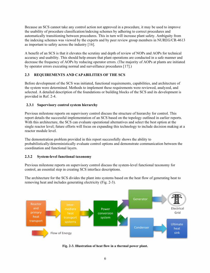
The architecture for the SCS divides the plant into systems based on the heat flow of generating heat to removing heat and includes generating electricity (Fig. 2-3).
Fig. 2-3. Illustration of heat flow in a thermal power plant.
Reactor and
primary heat
transport t
Inter‐mediate heat
transport systems
Power conversion system
Generator
Condenser Ultimate heat sink
Electrical Grid
Flow of Energy
7
Modular-designed, multi-unit plants have more and stronger dependencies among systems than single-unit plants at a common site. In fact, the design philosophy of the modular multi-unit plants is to form a single power plant station with respect to power generation and control. This philosophy is readily apparent with the single turbine-generator shared among three reactor modules for the ALMR PRISM power block.
Stand-alone units at multi-unit sites commonly share support systems and utility systems. However, because sharing of systems between reactor modules has increased, some heat removal systems may be shared at AdvSMRs. This introduces new management and control criteria at the organizational layer (i.e., power block level), coordination layer (i.e., local SCS control), and functional layer (i.e., reactor module level).
2.3.3 Human-machine interface
The SCS is designed to maintain plant parameters from reaching trip setpoints. The human-machine interface (HMI) functions to provide the operator with the proper interfaces to guide and direct the control system to operate in the proper modes. The HMI provides clear, key summary information to operators.
With no human intervention, the SCS must be able to detect and predict changing conditions and disturbances, to identify the best response(s) for actual or predicted plant conditions, and to continuously reevaluate operational status. The key question regarding control is, what is the appropriate level of automation for an AdvSMR?
The HMI functions can provide the operator with proper interfaces to guide and direct the control system through the use of a properly organized and managed alarm system. Alarms are classified to their severity and time response requirements to differentiate between long-term maintenance items and critical items demanding immediate attention. As the system moves away from the nominal state space, the status indication increases from alerts to alarms. 1F1F
2
If the system parameters progress into the degraded region of control, operator awareness and involvement with the SCS increases. The three levels of operator involvement, based on the scale of degrees of automation [20F18], are
1. nominal operating range: the computer decides everything and acts autonomously, with no need to inform the operator of actions taken. No operator’s response or intervention is needed. Sufficient monitoring information is available to the operator to confirm that the system is operating within the nominal operating range.
2. alerts: the computer determines a complete set of action alternatives, selects one, executes automatically, and then necessarily informs the operator.
3. operator alarm: the computer determines a complete set of action alternatives, selects one, and executes the selected alternative if the operator approves.
The SCS uses a graded autonomy to execute any decision, uses the alarm system to inform the operator of a decision (alert), or requests confirmation of a decision (alarm). In the nominal range, the SCS is fully autonomous and decisions are probabilistically informed. As the system progresses closer to a trip
2 An alert is a notification for the operator to be watchful and is lower priority than an alarm. An alarm indicates if and when the value or the rate of change value of a measured or initiating variable is out of limits, has changed from a safe to an unsafe condition, and/or has changed from a normal to an abnormal operating state or condition.
8
setpoint, autonomy decreases by informing the operator of what action was taken or requesting concurrence from the operator before an action is taken.
2.4 FUNCTIONAL ELEMENTS OF THE SCS ARCHITECTURE
The SCS functional architecture includes four key functional elements for decision making: 1. The probabilistic decision-making module, 2. The enhanced risk monitor (ERM) module, which provides diagnostics and prognostics
information, and 3. The performance-based decision-making module. 4. The utility theory algorithm to select a control option.
These modules are briefly described here; details about the mathematical models are provided in subsequent chapters. Fig. 2-4 shows the functional architecture of the SCS and illustrates how the decision-making block relates to the overall functional architecture.
9
Fig
. 2-4
. Fun
ctio
nal a
rch
itec
ture
of
the
sup
ervi
sory
con
trol
sys
tem
.
The SCS follows the process given below.
1. The SCS recognizes the component/system failure. 2. The SCS transmits component/system failure(s) or degradation to the probabilistic model.
Operating Procedures
Guidelines
Operating Experience
Y N
Dat
a A
cqu
siti
on
- A
cq
uir
e s
en
so
ry d
ata
Ver
ific
atio
n
- Te
st
solu
tio
n in
a
low
er-
ord
er p
lan
t m
od
el
Ac
tua
tio
n
- G
ener
ate
act
uat
ion
co
mm
and
Current Plant State Future Plant State
S1
S2
SN. . .
Data Bus
- In
terp
ret
se
ns
ory
da
ta
- D
ete
rmin
e p
rox
imit
y t
o c
ha
lle
ng
e s
urf
ac
e
- D
ete
rmin
e c
urr
en
t o
per
atin
g r
eg
ime
- P
erf
orm
tre
nd
s a
na
lys
es
Pla
nt
Sta
te E
stim
atio
n
- F
ailu
re d
iag
no
sis
- D
ete
ct
an
om
alie
s
- D
ete
ct
se
nso
r d
rift
an
d c
om
po
nen
t
de
gra
da
tio
n
- Id
enti
fy f
ault
in
cip
ien
ce
- Is
ola
te f
au
lts
- P
roje
ct
rem
ain
ing
us
efu
l li
fe e
sti
mat
es
- P
rob
ab
ilit
y o
f fa
ilure
vs
. tim
e h
ori
zon
- C
yc
le c
ou
nti
ng
Dia
gn
ost
ics
and
Pro
gn
os
tics
Lo
op
un
til C
on
verg
en
ce
MSCS
Operator Input
Des
ired
Fu
ture
S
tate
DE
CIS
ION
MA
KIN
G
EV
AL
UA
TIO
N
ME
TR
IC
De
cis
ion
An
aly
sis
IMP
LE
ME
NT
DE
TE
RM
INIS
TIC
PO
RT
ION
___
___
__
___
___
___
___
___
___
__
___
___
__
___
___
___
___
___
___
__
___
___
___
___
___
___
__
___
___
___
___
___
__
- C
he
ck g
en
era
ted
alt
ern
ativ
e s
uc
ce
ss
pa
ths
fo
r co
nfo
rmit
y t
o g
uid
elin
es
, etc
.-
Ra
nk
the
pa
ths
for
lik
elih
oo
d o
f s
uc
ces
s
< a
pp
ly u
tili
ty t
he
ory
>
- G
en
era
te a
sin
gle
so
luti
on
th
at r
ep
res
en
ts
an o
pe
rati
on
al s
tra
teg
y
De
cis
ion
Op
tio
ns
IMP
LE
ME
NT
PR
OB
AB
ILIS
TIC
PO
RT
ION
___
___
__
___
___
___
___
___
___
__
___
___
__
___
___
___
___
___
___
__
___
___
___
___
___
___
__
___
___
___
___
___
__
- R
efl
ect
fau
lt s
tate
in
th
e R
T-P
RA
mo
de
l
- R
efl
ect
dia
gn
os
tic
s a
nd
pro
gn
os
tic
s
ind
ica
tors
in
th
e R
T-P
RA
mo
de
l
< p
erf
orm
fa
ult
-tre
e a
na
lysi
s >
- G
en
era
te s
uc
ces
s p
ath
s t
o a
no
min
al
or
acc
epta
ble
sta
te
< p
erf
orm
eve
nt-
tre
e a
na
lys
is >
- N
av
iga
tio
n t
o m
ap
de
sir
ed
fu
ture
sta
te
on
to c
urr
en
t st
ate
10
3. The probabilistic model identifies those options with the greatest likelihood of avoiding a trip setpoint.
4. The probabilistically based success options are transmitted to the deterministic model in the form of a set of control actions.
5. The deterministic model evaluates the dynamic performance implications of the options based on current plant status.
6. Based on the probabilistic and deterministic assessments, the SCS selects a control option and initiates the corrective action, effectively executing the control actions.
2.4.1 Probabilistic decision-making module
The probabilistic decision-making engine acts on failed or degraded component information, as well as sensor and state information, to identify and rank control restoration actions. A list of possible actions is ranked based on the potential for success (or more generally on minimum expected utility) based on real-time plant equipment and state information. Based on plant operating status, component health, and equipment failures, the SCS decision-making capabilities use probabilistic analyses to identify a set of control options. If these options are implemented, they should prevent or minimize the likelihood of the actuation of the protection system. The possibility for one or more outcomes, based on component health and plant status, distinguishes probabilistically informed decision making from more traditional decision making. The probabilistic portion of the decision-making algorithm ranks the likelihood of success or minimizes the expected loss of each decision path based on the current system/plant status and component health. Based on the likelihood of the success metric under these conditions, the decision-making algorithm automatically chooses the top candidate control options as decision alternatives for executing the corresponding set of corrective actions. Selecting any of the control options would allow operations to continue by maintaining system status within the acceptable region. These actions and selection processes are similar to those an operator would be expected to perform except that the SCS has a much greater capability to consider and evaluate alternatives. Once the control options are identified and ranked based on their likelihood of success, the SCS transmits the highest ranking options to the deterministic portion of the platform (see Sect. 4).
2.4.2 Enhanced risk monitors module
The ERM module, represented with the diagnostics and prognostics box in Fig. 2-4, provides health information at the component level. The ERM framework was developed as a key element of overall enterprise risk management approach, where a proactive operations and maintenance (O&M) strategy is adopted to enable situational awareness. The ERM module keeps track of component health indicators such as probability of failure (with a confidence interval) and remaining useful life of individual ERM terminals conceptually located in close proximity to key components of interest. These terminals can be dedicated programmable logic controller (PLC)- or field programmable gate array (FPGA)-based devices that monitor variables of interest specific to a component or process. For instance, as described in Appendix D, variables of interest for a pneumatic valve may include valve position (i.e., position sensor output), rate of change of valve position (i.e., derivative of the position sensor output), and pressure of the gas in the upper and lower chambers, among others. The specific real-time ERM algorithm can be implemented at the hardware level, similar to a watchdog, to continuously generate the probability of failure and remaining useful life information for supervisory control decision making.
11
2.4.3 Performance-based decision-making module
A sufficiently detailed system model is essential in (1) evaluating the dynamic effect of the set of control actions identified as a result of the decision-making algorithm and (2) ultimately assessing whether the action set is acceptable for execution. The system model is based on the design specifications provided in the ALMR PRISM PSID. The outcome of the probabilistic module is a set of decision alternatives each of which may have a varying number of control actions. The probabilistic assessment ranks these alternatives according to their likelihood of success in terms of component condition and availability for a given decision trajectory. However, it does not indicate the potential consequences of these sets of actions dynamically on key process variables. Furthermore, certain instructions generated by the probabilistic model only include an abstract notion of action without specifications. For instance, one instruction may be to reduce power without specifying how much reduction is needed.
The purpose of performance-based decision making is to assess and rank each decision option by analyzing the dynamic performance implications of the individual decision branches. The performance-based decision making module receives inputs from the probabilistic decision-making module and the ERM module to generate a single solution. Interfaces to these modules are defined later in the section.
2.4.4 Utility Theory Algorithm to Select a Control Option
Within the supervisory decision-making framework, the ERM module functions as the trigger for the decision-making module. The data generated by individual field ERM terminals are acquired by the probabilistic decision-making module to update the event tree / fault tree (ET/FT) models using the most recent failure probability estimations. The objective of employing the utility theory is to create a framework by which the physical behavior of the system can be assessed as a function of a control trajectory—or a set of control instructions—along with the probabilistically ranked decision alternatives. The evolution of plant status is monitored by a set of state variables determined to be key actors in control. The objective of the deterministic decision-making module is to incorporate the current and projected physical behavior of the system. To achieve that capability, utility variables must be selected so that the projected physical behavior of the system can be factored into the decision making with the probabilistically ranked options from the PRA calculation. This is best accomplished by linking the desired utility attributes to key process variables (i.e., those that provide insight about the status of the system). Examples of system design variables for the ALMR PRISM and their nominal steady-state values include reactor thermal power, reactor inlet and outlet temperatures, and the difference between the inlet and outlet temperatures.
2.5 SOFTWARE IMPLEMENTATION OF THE SUPERVISORY CONTROL SYSTEM
The software requires different components written by PNNL and ORNL to work together. Fig. 2-5 shows the overall software architecture. Packages written by ORNL are shown in green, and packages written by PNNL are shown in orange. The interface package is shown in pale yellow. This figure provides a high-level view of the software architecture, conveys the programming language used for each package, and shows how the different components interface with each other. It does not convey how and what data flows between different modules.
12
The software modules have or require the following functionality: MainApplication: This application provides the graphical user interface and allows the user to
enter data to be sent for configuring and executing the other components. o Any input/output streams sent to or received from components are handled by the
PythonHandler component. o RWBHandler manages the data input and output (I/O) between the MainApplication
and the RWB model. Plant Model (ORNL): Simulates plant operation in normal and off-normal conditions, and
embeds supervisory control logic. This component receives initial conditions and solver settings from the user and returns the solution for all time- dependent variables in the plant model. Access to internal variables (at the different time steps as the simulation runs) is needed for integration purposes.
ERM Module (PNNL): Provides probabilities of failure (POFs) of plant components. Currently this component only implements a prognostic model for pneumatic valves. This requires measurement inputs related to valves and outputs remaining useful life (RUL) and POF. Note that the other elements (such as the predictive risk calculations and the economic/safety risk computation modules) are also available in Python but are not invoked in this version of the software being integrated into the ORNL SCS.
Interface (ORNL): A middleware utility used to route information from the MainApplication to the Prognostics component through the standard input/output streaming features. The purpose of this interface is to separate data transfer between components of different languages from the data. The MainApplication handles the data.
Probabilistic model (ORNL): Provides fault-tree and event-tree models for probabilistic decision-making; interfaces with the MainApplication for modifying component failure probabilities and execution of the model.
Fig. 2-5. Software elements of the supervisory control decision-making application.
13
3. PROBABILISTIC DECISION-MAKING MODEL
The use of a probabilistically informed approach in an SCS allows probabilistic insights to be coupled with other factors of concern such as magnitude from nominal set point, speed of parameter adjustment needed, etc. For example, a high outlet temperature from the reactor core can be lowered by decreasing power, reducing the coolant inlet temperature, or increasing secondary side flow rate. Each of these can be adjusted using plant controls. Inserting the control rods and increasing coolant flow are means to reduce core thermal power. Each control option has a different probability of success and can be linked to magnitude, speed, and other metrics of interest. For example, inserting the control rods will have a large, rapid effect on the output temperature, while changing pump speed on a feedwater pump will have a small, slow effect. To meet the objectives for the SCS, the following requirements of the probabilistic tools will allow winnowing the selection of probabilistic techniques to be considered. Specifically, the probabilistic techniques must be able to
address all component states (i.e., failed, OOS, degraded, operating), recognize changes in status for one or more components (up to all components) simultaneously, recognize changes in component status on a real-time basis (e.g., working to failed), recognize a change in probability of failure (e.g., to 1.0), and calculate different metrics of interest (i.e., measure the appropriate metric for the type of analysis
being performed, such as core damage frequency [CDF], challenge to safety system setting, etc.). Because linked FT/ET probabilistic analysis techniques can be used to evaluate the change of state for a component to be assessed (e.g., working to failed) but also allow combinations of component states to be evaluated simultaneously (e.g., component A fails, component B OOS), this technique was chosen for the decision module to be implemented in the SCS. Thus, the FT/ET models allow all possible combinations of component states to be evaluated simultaneously. With the SCS, this capability does not increase computational time. In most ETs, the success path is upward and the failure path is downward at each ET branch point. Although modeled the same in conventional ET models, the SCS is focused on the success paths of the ETs. Contributors to the path or sequence of avoiding a trip setpoint include elements such as the successful implementation of changing the status of a component (e.g., pump started, valve opened) so that SCS operation continues. The term probabilistic risk assessment (PRA) is often used to represent the methodology for the probabilistic portion of the SCS. That is, the standard PRA techniques of ETs and FTs to model system behavior are used, but they are used in a different way. When incorporated into a control system, the PRA is used to measure the likelihood of avoiding a trip setpoint (success space) rather than the likelihood of a plant transient (failure space). Used in this manner, the ET/FT models can reflect the failure of a component with any number of components OOS or in a stressed state (e.g., degraded state and thus with an increased failure probability). The computational time associated with the ET/FT models is independent of the number of components OOS, status if degraded, or its repair time. Furthermore, the models can identify multiple simultaneous control actions to be taken for a single option. To further differentiate the incorporation of a PRA into a control system from conventional PRAs, in this application the control system autonomously and automatically adjusts the ET/FT models based on actual plant conditions and recalculates the metric of interest.
14
3.1 CONTROL SYSTEM LOGIC MODELS
The probabilistic model is based on the simplified ALMR PRISM balance-of-plant (BOP) model, and it accurately represents redundancies to identify alternate heat rejection paths. The ultimate objective of the SCS is to keep the normal heat-rejection path operational to maintain operations within limits or to adjust reactor power to match heat rejection capabilities. The objectives of the SCS are to maintain steam flow to the turbine generator and FW flow to the SGs. The linked FTs track the status (including health) of the components. A component’s failure or unavailability is transmitted by the SCS to the FT, which then transmits that information to the ET. The IEs for the ET models are “challenges to successfully maintaining the heat balance from the reactor core to the ultimate heat sink.” The ET branches capture the logic of the equipment/components in the systems, and the FTs capture the operational states of those components (e.g., operating, maintenance, failed, or degraded). Thus, the ET/FT models capture the component/system/plant statuses of components working properly, in a degraded state, OOS, or failing. The logic model provided is for a plant at 100% power. The ET/FT models capture the actions that would be taken by an operator in the event of an upset (e.g., component failure) in the power conversion system for the ALMR PRISM, as shown in Fig. 3-1. With the system in operation, the steam generator block valves (SGBVs), when open, provide steam from the reactor/steam generator pair to the common steam header, eventually to the shared turbine generator.
Fig. 3-1. Secondary cooling system for the ALMR PRISM [5].
15
To test and verify the accuracy of the probabilistic models for the SCS, the status of the turbine control valves (TCVs) and feedwater (FW) flow control valves (FCVs) were captured in the ET/FT models. The control options for three scenarios reflecting the failures/degradations/OOS conditions for these valves are provided below. Scenario 1: TCV drifts in closed direction Control options:
1. Reactor trips on steam generator (SG) low water level (i.e., do nothing). 2. Successfully reposition TCV. 3. Open the turbine bypass valve to compensate in the short term; advise reactor operator (RO) to
reduce reactor power/correct TCV logic error. 4. If reactor 2 (1) is not at 100%, open reactor 2 SGBV; advise RO to reduce reactor 1 (2)
Scenario 2: SG 1 FW FCV drifts in closed direction Control options:
1. Reactor 1 trips on low SG level. 2. Open SG 1 bypass FCV, shut main FW FCV. 3. Advise RO to manually isolate SG1 main FW FCV; investigate valve logic error. 4. Decrease steam demand from SG 1 by adjusting the SG 1 turbine FCV in the closed direction and
lowering generated power. 5. Advise RO to reduce reactor 1 power/ investigate valve logic error /consider option 2. 6. Decrease steam demand from SG 1 by adjusting the SG 1 turbine FCV in the closed direction. 7. Increase steam demand from SG 2 by adjusting the SG 2 turbine FCV in the open direction. 8. Maintain generated power in the short term. 9. Advise RO to investigate valve logic error and adjust power on reactor 2.
Scenario 3: SG 1 FW FCV drifts in open direction Control options:
1. Reactor 1 trips on high SG level. 2. Attempt to shut main FW FCV and open SG 1 bypass FCV. 3. Advise RO to manually isolate SG1 main FW FCV. 4. Report valve logic error. 5. Increase steam demand from SG 1 by adjusting the SG 1 turbine FCV in the open direction. 6. Decrease steam demand from SG 2 by adjusting the SG 2 turbine FCV in the closed direction. 7. Advise RO to investigate valve logic error and adjust power on reactor 1.
Based on the three scenarios, two ETs and the corresponding FTs were developed to reflect the proper heat balance in the secondary cooling system:
1. steam flow to turbine within limits, and 2. cooling flow to SGs within limits.
A TCV drifting closed would reduce steam flow to the turbine. FW FCVs drifting open or closed would increase/decrease cooling flow to the SGs, resulting in overcooling/undercooling of the primary system. Failing to increase steam flow or decrease FW flow would result in a heat imbalance in the secondary cooling system and a reactor trip.
16
The ET for the operational decisions associated with Scenario 1 above, which is based on the steam flow to the turbine being within proper limits, is provided in Fig. 3-2. The ET captures plant operations with 0, 1, or 2 SGs in service. Fig. 3-2 shows SG1 and SG2 in operation (i.e., SGBV 1 and SGBV 2 are open).
Fig. 3-2. ET for steam flow to turbine with one steam generator in operation (Scenario 1).
An equipment failure or increased likelihood of failure as predicted using diagnostics and prognostics may be reflected in more than one ET branch. For example, if TCV 1 fails, its failure is noted for both SG 1 and 2 in operation and SG 1 in operation. Decision-making options include opening/closing the turbine bypass valves to dump heat to the condenser, reducing power, manually shutting down the reactor, and if a controlled shutdown fails, then initiating a plant scram via the RPS. The underlying FTs for the ET branches capture the component states, including their failure modes, their being OOS, or their being available for service but not in service (important for alternate flow paths). When using conventional PRA techniques, coupled FTs and ETs are deterministic with respect to the nodes represented in event sequence diagrams (ETs) and FTs in that they do not consider all possible combinations and permutations of sequences, timing, and order that could typically comprise these events. Control systems must be dynamic and capable of adapting to any perturbation, including dynamic manifestation of order, sequence, or timing of the types of things that could be manifested in ETs and EFs, including human error. For the SCS, the ETs and FTs use the same techniques, but the modeling philosophy and rules may be applied in a nontraditional manner. The principal difference is that the focus of safety-related PRAs is the likelihood of events leading to severe core damage. In contrast, the purpose of the analyses performed in
17
support of the SCS is to assess the likelihood of scenarios associated with alternative control actions that lead to success. The same tools—ETs and FTs—are used, but the objectives are different. Another difference in application of these tools is the use of fixed ETs in which an assumed order of events is predetermined in conventional PRA. This assumption simplifies the analysis but has limitations. Because control systems are by their nature dynamic, it is necessary to consider alternative control options that involve repeated branching and different order of events in a time continuous manner. For example, the ET in Fig. 3-4 shows that FW flow must be reduced, and reducing it to SG1 OR SG 2 is sufficient. Because these models address component health and components being OOS through the FTs, control decisions reflect actual plant status. Another difference is that although events may be mutually exclusive for conventional PRAs, they are not for a control system. For example, a component cannot be OOS and available at the same time. However, for the control system, what is important is the OR gate at the top of the FT branch. If a component is OOS, its unavailability is 1.0. (See Fig. 3-10 for an example of an OR gate and a HOUSE event.) Although it may appear that the component failure probability will add to this probability, a probability cannot be greater than 1.0, and thus the FT top event is 1.0. Transferring to the ET, this means that the likelihood of success using that component is 0.0. If the component is in service, its availability is 1.0, and the FT top event is the failure probability of the component (e.g., 10-4) because the mutually exclusive leg of the FT branch has a probability of 0.0. The likelihood of success for the ET branch is then 1 – 10-4.
3.1.1 Failure data
The detailed reliability information for the BOP components used in the FTs were compiled by ANL [21F19]. Table 3-1 lists the components evaluated. Each subsection of the ANL report (provided in Appendix A) contains an overview of the ALMR PRISM BOP component design, followed by a brief review of possible failures modes (or subcomponents/systems) and then a review of applicable reliability data.
Because the examples provided below depend on valves, the valve failure modes discussed in the ANL report are provided. Valves experience a variety of failure modes, as indicated by those listed in Table 3-2. Each valve type is not subject to all failure modes, as the failure modes that may occur are functions of the valve configuration and operating mechanisms.
Table 3-2. Valve failure modes
Failure mode Description Units FTO/C Failure to open/close - SOP Spurious operation h-1 ELS External leak small h-1 ELL External leak large h-1 ILS Internal leak small h-1 ILL Internal leak large h-1
18
FC Fail to control h-1
Data for the types of valves listed in Table 3-3 were used in the FTs.
The communication pathways between the SCS and the probabilistic models need to recognize the change in state of a component (e.g., failed, degraded, or OOS), transmit that change to the probabilistic models, automatically adjust and execute the models with the change of state, with the probabilistic results transmitted back to the SCS. All of these operations must occur without operator interface or direction. That is, the programming has to autonomously recognize and implement any change of state, execute the probabilistic models, and transmit the results back to the SCS. To create a probabilistic tool that would recognize failures and evaluate the consequences of those failures in real time, an application with a graphical user interface was implemented, which automatically transmits the faults to the process that handles the probabilistic model. The process is able to create new gates in the FTs, create new failure events, link the events to the gates, and as such can modify the probabilistic model as needed. Just as important, the data transfer pathway also transmits results of the probabilistic models that reflect the failure back to the SCS. The data transfer pathways for injecting a fault, instructing the probabilistic-risk-analysis software Reliability Workbench (RWB) to recalculate the metrics of interest, and transmitting the results back to the SCS were successfully completed. This meets the SCS requirement for automatic response. To meet the autonomous requirement, the SCS must be capable of making a decision based on current plant configuration coupled with a system or component failure. That is, once a fault or failure is detected, the SCS must determine what has failed and identify the control options to maintain the plant within the control boundaries. Because the SCS is not based on a priori decisions and is not executing the reliability software, it must reconstruct the ET, map the failure to the appropriate ET branch, and then deconstruct the ET to identify the control options at the component level as illustrated in Fig. 3-3.
19
Fig. 3-3. Sequence to identify probabilistically ranked control options.
3.2.1 Reconfiguration and execution of probabilistic models
Prior to the ET/FT models being reconstructed and deconstructed, they must first be updated to reflect actual plant status. For example, consider a TCV drifting close. The first step in identifying control options is for the coupled FTs and ETs to recognize that TCV is drifting close and to modify the probabilistic model to reflect the failure. In this example, a fault is injected to simulate the failure of the TCV. The SCS recognizes that the TCV is drifting close and changes the status of TCV in the FT model from operating to failed, as illustrated in Fig. 3-4. The SCS executes the probabilistic analysis with the current plant configuration models and stores the results in a relational database.
Fig. 3-4. TCV drifting-close status is communicated to the probabilistic model.
20
3.2.2 Reconstruction of ET from component failure
The ability to make a decision requires knowledge of the likelihood of success for the different control options given the failure that just occurred. Determining the likelihood of success requires knowledge of the event sequences, and it requires that the SCS reconstruct the ET/FT models. The sequences with the greatest likelihood of success can then be selected. In reconstructing the probabilistic model from the data, the SCS must recognize that the fault “TCV DRIFT” is entered into Gate “01-TCV” in the FT (Fig. 3-5): the SCS maps the basic event to the gate. 6
Fig. 3-5. FT reconstruction continues until ET branch link is identified.
After the fault is properly mapped to the FT, the FT must be mapped to the ET. The SCS must link the FT gate to an ET branch. At this point of reconstruction for this example, the SCS recognizes that the gate “01-TCV” is directly linked to an ET branch, and no further reconstruction of the FT is necessary. Other inputs to gate “01-TCV” are used to show TCV in/OOS (i.e., maintenance or repair) or in a degraded state. The SCS must once again link the FT gate to an ET branch. This time, the SCS links gate “01-TCV” to ET branch 1. Thus the SCS has the information that the component “TCV DRIFT” is linked to ET branch 1 through FT gate “01-TCV”. Now that the SCS has the information regarding where in the ET the failure occurred, it must reconstruct the ET so that any decision options can be identified. The SCS first recognizes that there are 16 ET branches in this example problem, as shown in Fig. 3-6 (i.e., 0–15). 8F
Fig. 3-6. ET branch numbers used to map FT to ET.
21
The next step in the reconstruction process is to actually reconstruct the ET to identify and quantify success paths. Beginning with the IE, the SCS reconstructs the ET. 9F In this example, branch ID EB-1 and EB-2 are initiator legs for TCV drifting close in ET branch 1. ET branch EB-2 represents the do nothing branch that ultimately leads to a reactor scram. ET branch EB-1 is the InputBranch to EB-3 and EB-4 in ET branch 2 (Fig. 3-7). Similarly, EB-4 is the InputBranch to EB-5 and EB-6 in ET branch 3. The process is completed for each ET branch until the ET reconfiguration is complete. This shows how the software links component names, FT gate names, and ET branches together to reconstruct digitally what is depicted in Fig. 3-7. The result is the same as the ET in Fig. 3-2.
Fig. 3-7. Reconfigured ET.
The ETs model one SG in operation (SG 1 or SG 2) or both SGs in operation (SG 1 and SG 2). In the example in Fig. 3-7, both SGs are in operation and hence any recovery actions are based on this mode of operation.
3.2.3 Deconstruction of ET to identify corrective actions
Now that the SCS has reconstructed the ET with the fault properly accounted for in the FT and ET, it must now deconstruct the ET to identify the control options for successfully maintaining system operation. The reconstructed ET shows there are four viable control options based on probability for avoiding a trip setpoint (Fig. 3-8).
22
Fig. 3-8. Deconstruction of ET to identify decision options.
The deconstruction process is used to first determine those actions that, if taken, would avoid a trip set point. Note that this is different than operations to continue producing power. To identify the control options for each sequence of events, the deconstruction process must alternate between the ET and FTs and must check the status of components to ensure they are available if needed or to acknowledge that they are unavailable. In this example, the deconstruction starts with ET branch 15 (Fig. 3-8) and deconstructs the ET, branch by branch, until it has collected, reviewed, and identified options back to the ET branch where the fault occurred. In this example it is ET branch 1. In deconstructing the ET, the SCS must automatically and autonomously determine that there are five success paths, each with the potential control commands at the success/failure branch points on the ET. Success paths with decision points are provided in Table 3-4.
Table 3-4. Control options identified from deconstruction process
Likelihood of success
ET branch sequences(s)
Control option Consequence
1.0 1 Do nothing Scram reactors 0.8999 14 Controlled shutdown of Rx1 50% power 0.8902 6–10 Reduce FW flow; reduce power Power reduction 0.887 8–10–12 Open TBV; reduce power; close TBV Power reduction 0.1 2 Successfully reposition TCV 100% power
23
Within each ET success sequences are the SCS control commands embedded within the linked FTs (Fig. 3-9). The format of the control commands relays the actions to take to the SCS to avoid a trip setpoint for each of the sequences under consideration. The format providing the information for each control signal includes:
a house event (i.e., 1.0) identifier signifying that this is a control signal, the lead identifier in the house event (i.e., SCS) means that the following information is an SCS
command signal, and the component and the action to be taken.
Fig. 3-9. Deconstruction of ET branch 14 identifies SCS command signals for successfully avoiding a trip setpoint.
As an example, the house event SCS shutdown Rx1 in Fig. 3-9 tells the SCS to perform a controlled shutdown of reactor 1. The other command associated with shutting down reactor 1 is to close the SGBV associated with reactor 1 (i.e., house event SCS SGBV 1 CLOSE). Not shown in the example above is that the FTs account for equipment degradation, fault, and OOS conditions, as well as associated SCS actions (Fig. 3-10). FTs capture availability of component, component health, control option(s), component failures, and maintenance (OOS).
24
Fig. 3-10. FTs capture component failure and carry SCS control instructions (OOS).
The SCS successfully recognizes the existence of a fault, automatically evaluates the operational alternatives available, and generates a list of probabilistically ranked decision alternatives. These alternatives are automatically fed back to the SCS module which forwards these options to the dynamic system model.
3.3 INTERFACES TO ENHANCED RISK MONITORS (ERM) MODULE
The ERM module developed by PNNL provides the failure probability estimations for key plant components modeled in FTs as illustrated in Fig. 3-11. The probability of failure estimation generated by a particle filter model, which will be briefly discussed in Appendix D, also provides an uncertainty bound around the expected value.
Fig. 3-11. Interaction between the ERM module and the probabilistic decision-making module.
ERMs are capable of providing predictive estimates of the probability of failure (POFs) of monitored components, as well as the associated predictive risk to system operation. Such information is likely to be of value to supervisory control algorithms, as knowledge about potential failures can be used to make operational decisions. The ERM framework developed by PNNL consists of three major functional modules that use sensor measurements and provide predictive estimates of component failure
25
probabilities, operational risk, and associated uncertainties. Functionally, these modules may be integrated with the supervisory control framework to provide the necessary diagnostic and prognostic information upon which the control decisions are made. In addition, information on risk to system operation is likely to be of value in the decision-making process, but such information is not expected to be used at the initial stages of integration and testing. The value of integrating the ERM into a supervisory control framework is shown in the example below (Fig. 3-12). In this example, the FW FCV is in service and operating normally. The ERM recognizes that the FW FCV for SG1 is in a degraded state and transmits an updated failure probability to the SCS. The SCS modifies the FT, which is linked to the ET. The ET/FT models automatically identify the success paths for the current plant status and transmit this back to the SCS (Fig. 3-13).
Fig. 3-12. Probabilistic model updated based on ERM monitoring.
26
Fig. 3-13. Order of probabilistic options changes with degraded FW FCV.
Table 3-5 shows that the monitoring of a component’s health via the ERM may result in re-ranking of probabilistic options. In this example, the reduce FW flow—reduce power and the open TBV—reduce power—close TBV options switched order for the likelihood of success. This is because in this example, the FW FCV is operating in a degraded condition and is less likely to operate successfully.
Table 3-5. Re-ranking of control options based on changing component health
Before: Degraded FW FCV: 1. Do nothing 1. Do nothing 2. Controlled shutdown of Rx 1 2. Controlled shutdown of Rx 1 3. Reduce FW flow; reduce power 3. Open TBV; reduce power; close TBV 4. Open TBV; reduce power; close TBV 4. Reduce FW flow; reduce power 5. Successfully reposition TCV 5. Successfully reposition TCV
3.4 RESULTS OF PROBABILISTIC MODELS
FT/ET models were created to identify and rank acceptable control actions in the order of likelihood of success. ET/FT models measure the likelihood of successfully controlling the heat balance in the secondary system given the operation of one or two reactors. Because the SCS communicates with the FT/ET models automatically and autonomously, the control options based on the likelihood of success are provided back to the SCS in real time. The reconstruction/deconstruction for Scenario 1, TCV drifts in closed direction, is described above. This process for Scenario 2, SG 1 FW FCV drifts in closed direction, is described in Appendix C.
27
A probabilistic model overcomes the limitations of other modeling techniques as follows: The model is dynamic because the time sequence of events and control options is captured in the
models. Any failure/fault/outage (component status) can be injected into the model. The faults are not hard-wired into the code; the consequences of the faults do not need to be
determined a priori. The model is automatically reconfigured. After reconfiguring, the models execute automatically. The results from the probabilistic analysis are automatically provided to the user (e.g., assessment
of the impact of the failure or the likelihood of the metric of interest occurring). The technology is independent of the metric of interest as detailed below:
Any model and metric can be evaluated. The metric of interest can be core damage frequency (safety) or challenges to reactor protection
system (operations).
29
4. PERFORMANCE-BASED SYSTEM MODEL
A sufficiently detailed system model is essential in evaluating the dynamic effect of the set of control actions identified as a result of the decision-making algorithm and ultimately assessing whether the action set is acceptable for execution. The system model is based on the design specifications provided in the ALMR PRISM Preliminary Safety Information Document (PSID) [5]. The ALMR PRISM dynamic model was implemented in Modelica language on Dymola platform. The model is based on the open-source simulation framework “Transient Simulation Framework of Reconfigurable Modules (TRANSFORM),” which was also funded under the DOE Advanced Reactor Technologies (ART) program within the ICHMI technical area. Further details about TRANSFORM can be found in Ref. 83F22F20. The end-to-end system model provides a detailed account of an ALMR PRISM power block, which contains three reactor modules, each connected to its own steam generator, and three steam generators driving a single power conversion system through a common header. The top-level diagram view of the hierarchical model is shown in Fig. 4-1.
Fig. 4-1. Top-level diagram view of the ALMR PRISM power block.
A brief description of the subsystem models is provided below for completeness. While there are some improvements in individual subsystems, the most significant improvement is introduced in the power conversion system to capture necessary dynamics of key disturbances and to allow for the needed interfaces to control.
4.1 REACTOR AND PRIMARY HEAT TRANSPORT SYSTEM
Each reactor and the primary heat transport system (PHTS) models include a six-group point kinetics model (average heat source), average flow channel models for the driver, blanket and shield regions of the core (heated and unheated vertical sections), and the flow models for the downcomer, cold pool, lower and upper plena, and the cover gas. The electromagnetic (EM) pump is not explicitly modeled because it
30
is assumed to provide a constant flow rate for the PHTS. The number of axial nodes in the flow channels can be specified by the user. The diagram layer of the PHTS model is shown in Fig. 4-2.
Fig. 4-2. Reactor and primary heat transport system model for ALMR PRISM.
Each zone is represented by three sections: the lower unheated section, the upper unheated section, and a heated section corresponding to the active fuel region. Each section includes a heat source represented by the ReactorKinetics object that models point kinetics, a FuelModel object that models radial and axial heat conduction, and a CoolantSubchannel object that models coolant flow, which is sodium in this case. The flow channels solve for mass, momentum, and energy conservation equations, as well as appropriate closure relations for wall friction and heat transfer. The diagram layer for each channel is shown in Fig. 4-3. For unheated sections, the reactorKinetics power level is set to zero. The fuel conduction model properly models the fuel, the sodium bond, and the cladding. The user can choose from a multitude of material options, including metal and oxide fuel, as well as different alloy options for cladding. These are defaulted to U-Pu-Zr for fuel, sodium for gap, and HT9 steel for ALMR PRISM cladding.
31
Fig. 4-3. Diagram layer for the reactor kinetics and coolant subchannel.
4.2 INTERMEDIATE HEAT EXCHANGER AND INTERMEDIATE HEAT TRANSPORT SYSTEM
The ALMR PRISM IHX is modeled by two flow elements interacting through a tubewall element as illustrated in Fig. 4-4. Consistent with the ALMR PRISM IHX description, the primary sodium flows in the shell side, while intermediate sodium flows in the tubes. The Tubewall object solves two-dimensional heat conduction equation in cylindrical geometry using the finite difference method. The flow channels solve for mass, momentum, and energy conservation equations, and the appropriate closure relations for wall friction and heat transfer.
Fig. 4-4. Diagram view for the ALMR PRISM IHX.
The tube side is modeled by a number of parallel straight pipes. The model also accounts for tube sheet entrance and exit effects. The shell-side flow and heat transfer correlations are derived based on the Bell-Delaware design method, in which the shell-side is divided into a number of sections. Pressure drop terms in the nozzles, baffle windows, central and end cross-flow sections, as illustrated in Fig. 4-5, are individually modeled [23F21].
32
Fig. 4-5. Elements of the shell-side pressure drop.
The diagram layer of the shell side of the IHX is shown in Fig. 4-6. The number of baffles can be specified by the user; it is defaulted to seven for the ALMR PRISM IHX.
Fig. 4-6. Diagram view for the ALMR PRISM IHX shell-side flow paths.
33
Each of the ALMR PRISM intermediate heat transport systems (IHTSs) were modeled with two pipes, one hot and one cold legs, as well as a 100% capacity pump, a sodium expansion tank, and a connecting line, as shown in Fig. 4-7.
Fig. 4-7. ALMR PRISM intermediate heat transport system layout.
4.3 STEAM GENERATOR SYSTEM
Each steam generator system (SGS) loop consists of a vertically oriented shell-and-tube heat exchanger, a steam drum, and a recirculation loop with a pump. The diagram layer of the model is shown in Fig. 4-8. Each SG model includes a main steam isolation valve (MSIV) and a steam generator block valve (SGBV) to allow isolation of steam flow into the high-pressure turbine through the common header. The recirculation ratio was set to 1.2 per the specification in ALMR PRISM PSID [5].
34
Fig. 4-8. Diagram layer for the ALMR PRISM steam generator and drum model.
The SG heat exchanger model resembles that of the IHX model as shown in Fig. 4-4, except the intermediate sodium flows are on the shell side, and water/steam flows inside the tubes from the SG (i.e., reversed from the IHX). Double-wall tube construction is properly modeled consistent with the design description. This steam drum on top of the SG is cylindrical and is connected to the outlet of the heat exchanger (SG) where steam flows through the riser. The Drum object uses a nonequilibrium thermodynamic model between the liquid and vapor phases. The drum model is based on dynamic mass and energy balance equations of the liquid and vapor volumes inside a cylindrical tank. Mass and energy transfer between the two phases is provided by bulk and surface condensation of the vapor phase and by bulk boiling of the liquid phase as illustrated in Fig. 4-9. Additional energy transfer can occur at the surface if the steam is superheated.
35
Fig. 4-9. Illustration of key phenomena in the steam generator steam drum model.
The riser flowrate is separated before entering the drum at the vapor pressure. The saturated liquid fraction goes into the liquid volume, and the wet vapor fraction goes into the vapor volume with a steam quality depending on the liquid/vapor density ratio. The pressure at the downcomer connector is equal to the vapor pressure plus the liquid head.
4.4 POWER CONVERSION SYSTEM
The ALMR PRISM PCS includes too many components to be represented in both the probabilistic model and the system model. Some simplifications in the models are as follows:
1. Two moisture separator and reheaters are modeled as a single component supplying identical steam to each low-pressure turbine.
2. Steam jet air ejectors are not modeled. 3. Steam packing exhausters are not modeled. 4. Blowdown processes (i.e., blowdown flash tank and blowdown coolers) are not modeled. 5. Four low-pressure feedwater heaters (LP FWHs) are represented by a single heat exchanger. 6. The redundant LP FWH train is not modeled. 7. Feedwater booster pumps and feedwater pumps are modeled as a single component; three
redundant trains are maintained. These simplifications have little to no effect on the thermal-hydraulic models and are accounted for in the probabilistic models through the use of super events that are represented as basic events. The SG isolation and turbine stop, control, and bypass functions are simplified as shown in Fig. 4-10. Similarly, the feedwater block, control, bypass and isolation functions are introduced consistent with ALMR PRISM PCS design, as shown in Fig. 4-11.
36
Fig. 4-10. Drawing that shows the three main steam lines, the common header, the turbine stop valve, and the turbine control valve.
Fig. 4-11. High-pressure FWH and connecting lines to steam generator drains.
37
The simplified PCS model developed in Modelica for the supervisory control project is shown in Fig. 4-12. This model contains a high-pressure turbine, a moisture separator and re-heater, two low-pressure turbines, a generator, a condenser, three condensate pumps, a low-pressure feedwater heater (FWH), a deaerator, three booster pumps, a high-pressure FWH, and the necessary valves for control, isolation, and bypass. This model is simplified in that it combines four low-pressure FWHs into a single FWH. This simplification was needed to match the system model to the probabilistic model. The PCS model also provides the necessary control and isolation interfaces for each individual steam generator.
Fig. 4-12. ALMR PRISM power conversions system model layout.
4.4.1.1 Feedwater heaters
The PCS model in Fig. 4-12 provides the necessary interfaces to manipulate the turbine FVCs, the low-pressure and high-pressure FW FCVs, recirculation flow control set points, and low-pressure and high-pressure FW pump controller set points. Currently the main steam isolation valve (MSIV) has not been modeled. The primary function of the MSIV is to redirect the main steam to the condenser in the event of a turbine or reactor trip. It is a safety-related component functionally isolated from the SCS. However, the MSIV must be included to demonstrate a key trip function in the event of a trip set point violation. The FW heater model closely resembles a RELAP5 FW nodalization scheme as shown in Fig. 4-13. While the FW flows on the tube side of a horizontal shell-and-tube heat exchanger and is slowly heated up, the extracted steam flows on the shell side and condenses. Because of the condensation, the shell side has a mixture of saturated water and steam. The water level is typically tracked by a dedicated control system for proper component operation. Although it has not been demonstrated, these control features are considered important in providing the SCS with ample options for decision making.
38
Fig. 4-13. Typical nodalization example of a horizontal feedwater heater in RELAP5.
4.4.1.2 Moisture Separator and Reheater
The moisture separator includes dynamic models of an ideal vapor/liquid separator and a horizontal heat exchanger with boiling inside tubes and condensation on the shell side.
4.4.1.3 Deaerator
The deaerator model is a horizontal cylindrical tank that assumes thermodynamic equilibrium between liquid and vapor phases as illustrated in Fig. 4-14. The metal wall dynamics is taken into account with a uniform temperature assumption. Heat transfer takes place between the metal wall, the two-phase fluid, and the exterior. A dynamic wall model is included if a non-zero metal heat capacity is defined. The condensate level is allowed to vary between and .
Fig. 4-14. Key phenomena in the deaerator model.
4.4.1.4 Condenser
The condenser model includes a three-zone heat exchanger as shown in Fig. 4-15. Cooling water and steam/condensate are separated by a dynamic wall model. The three zones make it possible to simulate subcooled and superheated phases.
39
Fig. 4-15. Temperature profiles of condensate and feedwater in a three-zone condenser.
The ALMR PRISM PSID provides details for major plant structures, systems, and components, but design data for the turbine side are limited, as no detailed information is provided for the sizes of components such as FWH heat exchangers, pumps, and valves. A detailed design of the ALMR PRISM PCS is not part of the project scope, so the ORNL team is using the available data in the ALMR PRISM PSID and filling in missing data with minimal design work and engineering judgement. Hence, component sizing is expected to be suboptimal. However, while the suboptimal configuration affects the overall thermodynamic efficiency of the system, it is not expected to have a major impact on general system trends.
4.5 CONTROL SYSTEMS
This section describes the subsystem- or component-level continuous-time control systems. A high-level diagram of sensing and actuation interfaces for ALMR PRISM power block is shown in Fig. 4-16.
40
Fig. 4-16. High-level sensing and actuation interfaces for the ALMR PRISM power block.
4.5.1 Level control
Control models have been developed to regulate the level in (1) the steam generator drum, (2) high-pressure FWHs, (3) low-pressure FWHs, (4) the moisture separator and reheater, and (5) the condenser. As an example, steam generator level control is achieved by modulating the feedwater control valve (FCV) using the steam flow rate and feedwater flow rate as inputs. Generically, two control system options are made available: simple feedback control with a proportional-integral (PI) element (Fig. 4-17) and a combined feedforward and feedback control (Fig. 4-18).
Fig. 4-17. Level control system with feedback path only.
41
Combined feedforward and feedback control can significantly improve performance over simple feedback control when there is a major disturbance to be measured before it affects the process output. Even when there are modeling errors, feedforward control can often reduce the effect of the measured disturbance on the output better than that achievable by feedback control alone. Level control performance is significantly improved using a combined feedback and feedforward control system.
Fig. 4-18. Level control system with feedforward and feedback paths.
The simplest feedforward transfer function is obtained by taking the inverse of the response function of the process to be controlled. For instance, this is achieved for the high-pressure FWH by taking the inverse of the response function of the regulation valve, and for the low-pressure FWH, it is accomplished by taking the inverse of the pressure head vs. mass-flow-rate relationship of a centrifugal pump.
43
5. UTILITY THEORY ALGORITHM USED TO GENERATE A DECISION
The outcome of the probabilistic module is a set of decision alternatives, each of which may have a varying number of control actions. The probabilistic assessment provides a ranking of these alternatives, called a likelihood of success, in terms of component condition and availability for a given decision trajectory. However, it does not provide an indication about what potential consequences of these sets of actions would be dynamically on key process variables. Furthermore, certain instructions generated by the probabilistic model only include an abstract notion of action without specifications. For instance, one instruction may be to reduce power without specifying how much reduction is needed.
The purpose of performance-based system models is to assess each probabilistically identified control option by considering the dynamic performance implications of the individual probabilistically identified control options. The performance-based decision making module receives inputs from the probabilistic decision-making module and the ERM module.
The results from the probabilistically identified control options and the performance-based system models are used to generate a single solution using utility theory. Utility theory provides a methodological framework for evaluating alternative choices. In this context, utility is defined as the satisfaction that each choice provides to the decision maker. Hence, utility theory assumes that any decision is made on the basis of the utility maximization principle, which states that a rational decision-maker selects a set of options that maximizes benefit. Utility maximization is considered a type of optimal decision problem.
The advantage of using utility functions is that multiple criteria can be weighed against one another. The simple additive weighting (SAW) method, one of the most widely used scoring methods, was used to weight, score, and select a control option. A score in the SAW method (Eq. 5-1) is obtained by adding contributions from the individual utility attributes, ∈ 1,… , , into a compound utility metric, , for the decision branch by the following expression:
(5-1)
where
is the likelihood of success associated with the th branch of the decision tree,
is the total number of utility variables (e.g., nine utility attributes were identified for ALMR PRISM),
is the utility weight of each utility function, and
is the utility function for the attribute .
The decision branch with the highest compound utility, , is selected.
The compound utility is calculated based on the maximum or minimum values taken by process variables, which is determined based on a detailed, end-to-end dynamic simulation of the plant. Through the normalization process, each incommensurable attribute becomes a pseudo-value function, which allows direct addition among alternatives.
44
The compound utility may also be calculated as a time-varying variable, , for the decision branch at time step by the following expression (Eq. 5-2):
. (5-2)
For a time-varying utility evaluation at a decision node, the lowest compound utility value of a decision branch must be used for decision analysis. This is the method used in the SCS decision-making demonstration.
5.1 LIKELIHOOD OF SUCCESS
The probabilistic decision-making evaluation (repeated in Fig. 5-1) generated a total of five decision paths for consideration. Each path is linked to a branch in a decision tree with a likelihood of success metric as represented in the last column of the ET and a series of control actions identified by the FTs linked to the top events.
Fig. 5-1. Decision paths generated through ET evaluation.
More specifically, the performance-based decision-making module receives the following input from the probabilistic decision-making module:
1. number of decision alternatives or decision branches,
2. likelihood of success for each decision alternative, and
3. individual set of control actions for each decision branch.
45
While the probabilistic decision-making module automatically generates a set of control actions for each decision branch, it does not specify the performance parameters for a component associated with a control action. This is an important feature of the ERM module: as it monitors a component, it can detect and isolate a fault, which is performance degradation and its associated failure mode.
This requires that detected performance degradation be translated to new set of operational parameters for a component. For example, a valve is typically modeled with a flow coefficient, , which is a relative measure of its efficiency at allowing fluid flow. The flow coefficient describes the relationship between the pressure drop across an orifice, valve, or other assembly, and the corresponding flow rate.
The system model includes key components of subsystems such as pipes, pumps, or valves with nominal performance specifications. However, as components age, they naturally drift from their nominal specifications. It is important to map degraded performance to a new performance specification. For instance, for a valve, it might be a modified flow coefficient. Other performance parameters may also be required, such as actuation response times including the time to open or close a valve, or time to start or stop a pump. Furthermore, certain failure modes may require additional translations, such as upstream or downstream leakage rates. If these phenomena are important for a given performance evaluation, they must be properly included in the system model. These performance specifications are not currently generated by the ERM module, and they are beyond the scope of this work.
In summary, the performance-based decision-making module receives the following input from the ERM module:
1. performance specifications for each component associated with a control action,
2. actuation response-time specifications, and
3. remaining useful life.
The system model component parameters are updated with the estimated performance and response-time specifications during instantiation of the model.
5.2 UTILITY VARIABLES
The objective of employing the utility theory is to create a framework by which the physical behavior of the system can be assessed as a function of a control trajectory: a set of control instructions, along with the probabilistically ranked decision alternatives. The evolution of plant status is monitored by a set of state variables determined to be key actors in control. The objective of the deterministic decision-making module is to incorporate the current and projected physical behavior of the system. To achieve that capability, the utility variables must be selected so that the projected physical behavior of the system can be factored into the decision making with the probabilistically ranked options from the PRA calculation. This is best accomplished by linking the desired utility attributes to key process variables, which are those providing insight on system status. A partial list of system design variables for ALMR PRISM and their nominal steady-state values are shown in Table 5-1.
46
Table 5-1. ALMR PRISM heat transport system design values
Variable Description Nominal
value Unit
Reactor thermal power 425 MWt Reactor outlet temperature 468.3 °C Reactor inlet temperature 321.1 °C Reactor temperature difference 147.2 °C
Primary coolant mass flow rate (total) 2016 kg/s
, Primary pump discharge volumetric flow rate* 0.66 m3/s Primary pump head 96.3 m Intermediate hot leg temperature 426.67 °C Intermediate coolant mass flow rate (total) 2268 kg/s
, Intermediate pump discharge volumetric flow rate 2.6 m3/s Intermediate pump head 95.7 m Steam generator thermal power** 432 MWt
, Steam generator outlet temperature 285 °C
, Steam generator outlet pressure 6.895 MPa
, Steam generator feedwater temperature 216 °C Steam flow rate 233.5 kg/s
* Volumetric flow rate per pump; total of four pumps ** Includes pump heating from primary loop, intermediate loop, and steam generator pumps (~ 6.82 MWt)
The selection criteria for utility variables must address the safety envelope of the controls domain. As illustrated in Fig. 2-2, the fundamental objective of the SCS is to maintain the plant’s state within the controllable domain delineated by the red line, which is referred to as the challenge surface. In its simplest form, the challenge surface is formed by the trip variables that, if exceeded, initiate an RPS and/or ESFAS actuation. Reactor safety functions and associated trip variables for ALMR PRISM are listed in Table 5-2. During normal operation, the SCS functions in order to confine the plant state within an even tighter domain, which is delineated by the blue line in Fig. 2-2—also called the homeostatic region. Similarly, to incorporate a broader snapshot of the plant state, additional utility attributes must be linked with key process variables.
Table 5-2. Reactor trip variables and associated safety functions for ALMR PRISM
Safety function Monitored variable Type
Flux Monitor for insertion of reactivity (threshold function of operating power level)
Reactor core neutron flux TRIP
Flow Monitor for loss of flow* Primary loop sodium level
TRIP Primary loop EM pump discharge pressure
Temperature Monitor for loss of heat sink Reactor core outlet temperature
TRIP Cold pool temperature
Level Monitor for loss of sodium Primary loop sodium level TRIP
Pressure Monitor for electromagnetic (EM) pump outlet duct failure
Primary loop EM pump discharge pressure
TRIP
* The loss-of-flow measurement is indirect, using the EM pump discharge pressure as an indicator of the primary loop flow rate.
47
ALMR PRISM RPS actuates on the following trip variables [5]:
1. measured reactor core neutron flux ( ),
2. reactor core outlet temperature ( ),
3. cold pool temperature ( , ),
4. pump discharge pressure ( ), and
5. primary heat transport system (PHTS) sodium level ( ).
In addition to the RPS trip variables, the following were identified as important decision variables:
1. reactor core coolant temperature difference ( ),
2. intermediate heat transport system (IHTS) sodium level ( ),
To maintain consistency among the attributes, utility variables are derived from the process variables through a simple linear transformation (Eq. 5-3):
(5-3)
where
is the utility variable for the ith attribute and
is the process variable linked to ;
subscripts min and max are the minimum and maximum values each process variable is allowed to take (red line in Fig. 2-2).
For safety-related variables (i.e., trip variables) these values are obtained by the setpoints of their processes from plant technical specifications.
A preliminary list of utility variables selected for the supervisory control system for the ALMR PRISM based on the nine variables identified above is shown in Table 5-3.
48
Table 5-3. Process utility variables for ALMR PRISM supervisory control system
Utility variable
Safety variable
Min. Lower bound
Nominal Upper bound
Max. Linear transformation
(ºC) 132.2 142.2 147.2 152.2 162.2
(ºC) 453.3 463.3 468.3 473.3 483.3
(ºC) 306.1 316.1 321.1 326.1 336.1
(kPa) 807 817 827 837 847
(m) 9 10 12 14 15
(m) 2 3 5 7 8
(m) 2 3 5 7 8
(n/cm2s) TBD TBD TBD TBD TBD TBD
(kg/s) 242 262 272 282 302
5.3 UTILITY WEIGHTS
Selection of weights can significantly change the result of a decision calculation. A review of alternative weights is provided in Ref. 24F22. The Uniform Weight Distribution approach puts equal emphasis on each utility. The weights can then be calculated by (Eq. 5-4)
1 (5-4)
which leads to (Eq. 5-5)
1∀ ∈ 1, . . , (5-5)
5.4 UTILITY FUNCTIONS
The characteristics of utility functions are a subject of research. The shape of a utility function has implications for its effect on the overall decision. While utility functions presented in the literature—mostly in the field of economics—are expected to satisfy certain criteria such as monotonicity, non-decreasing, or strictly increasing properties, these rules result from the field of the application.
49
Engineering applications of utility theory expand the classical definition of utility functions to address specifics needs and requirements. For instance, Ref. 25F23 employs normal distributions for representing the relationship between a utility attribute and its functional form for decision-making on lane change.
The proposed selection scheme of utility functions greatly expands its definition:
1. Utility variables are defined in ∈ 0, 1 , which maps an engineering variable operating range between its minimum and maximum value.
2. Utility functions have a mean value of 0.50 (symmetry rule).
3. Utility functions intersect the abscissa at a lower-bound and an upper-bound value of an engineering variable.
4. Utility functions are positive within the domain delineated by the lower- and upper-bound, and they are negative elsewhere.
This scheme allows for rewarding a particular utility for being contained within the operations domain while penalizing it for being outside. Depending on the other parameters used, the penalty for not being contained within the domain can be significant, as illustrated below.
The probability density function of a normal distribution (Eq. 5-6) is represented as
| ,
, (5-6)
where
is the mean, and
is the standard deviation of the distribution.
Some examples from the family of distributions are provided in previous status reports.
The utility functions are selected from the family of Gaussian distributions through a linear transformation (called affine transformation) represented by Eq. (5-7),
| , (5-7)
where and are the coefficients of the transformation.
The intersection points are determined based on the lower- and upper-bound values of a safety variable. For instance, the lower- and upper-bound values for are determined as follows (Eq. 5-8a 5-8b):
(5-8a)
(5-8b)
50
Based on the values given in Table 5-3, these are calculated as
13
23
and values are symmetrical about 0.5, as illustrated with and .
The and values of the linear transformations shown in Eq. (5-7) for a given utility function | , are calculated by solving the following set of equations (Eq. 5-9a 5-9b):
exp2
(5-9a)
1 (5-9b)
As an example, solving Eqs. (5-9a) and (5-9b) for 0.5 and 0.15 yields
2.171117
1.171117
Again, the a and b values are generated based on the lower and upper bounds of the process variables and are the coefficients of the transformation. This transformation essentially determines the point where the curve intersects the abscissa. The utility functions for the ALMR PRISM process variables are generated based on this transformation.
51
6. DEMONSTRATION OF A SUPERVISORY CONTROL SYSTEM
This chapter demonstrates the SCS decision-making process that couples probability, performance, and diagnostics for Scenario 1 of the TCV drifting in the closed direction (Section 3.1). The probabilistic model for Scenario 2, “SG1 FWCV drifts in closed direction” is discussed in Appendix C. No models were developed for Scenario 3, “SG1 FWCV drifts in open direction.” The demonstration problem for the integrated decision-making process primarily focuses on the BOP of an ALMR PRISM power block. More specifically, supervisory control assessments are made based on the condition of three components: turbine control valve, TControlValve that controls steam flow to the turbine or to the condenser, and feedwater control valves—FWControlValve_1 and FWControlValve_2—that control the feedwater flow rate to steam generators 1 and 2, respectively, as illustrated in Fig. 6-1.
Fig. 6-1. BOP components monitored by the ERM functions for SCS demonstration.
To test and verify the accuracy of the probabilistic models for the SCS, the status of the TCVs and feedwater FW flow control valves FCVs were captured in the ET/FT models. Control options for Scenario 1 reflecting the failures/degradations/OOS conditions are provided below.
52
Scenario 1: TCV drifts in closed direction Control options:
1. Reactor trip on steam generator (SG) low-water level (i.e., do nothing). 2. Successfully reposition TCV. 3. Open the turbine bypass valve to compensate in the short term; advise RO to reduce reactor
power/correct TCV logic error. 4. If reactor 2 (1) is not at 100%, open reactor 2 SGBV; advise RO to reduce reactor 1 (2);
A TCV drifting closed would reduce steam flow to the turbine. FW FCVs drifting open or closed would increase/decrease cooling flow to the SGs, resulting in overcooling/undercooling of the primary system. Failing to increase steam flow or decrease FW flow would result in a heat imbalance in the secondary cooling system and a reactor trip.
6.1 PROBABILISTICALLY IDENTIFIED CONTROL ACTIONS
The difference between a probabilistically-informed and a probabilistically-based decision-making algorithm is that a probabilistically-based algorithm would simply select the option with the greatest likelihood of success without any other factors being considered. This may not be the best choice based on other criteria. For example, the most likely option for avoiding a trip set point probabilistically could be to manually shut down the reactor, but deterministic factors such as reduced generation of heat (i.e., power reduction) might re-rank this option to the least favorable of the choices. The ET for the operational decisions associated with Scenario 1 above, which is based on the steam flow to the turbine being within proper limits, is provided in Fig. 6-2. The ET captures plant operations with 0, 1, or 2 SGs in service, and this demonstration problem is showing two SGs in operation. The SCS automatically and autonomously determined that there are five success paths, and each success path has potential control commands at the success/failure branch points on the ET (Table 6-1):
Table 6-1. Control options identified from deconstruction process
Rank Likelihood of success
ET branch sequences(s)
Control option Consequence
1 1.0 1 Do nothing Scram reactors 2 0.8999 14 Controlled shutdown of Rx1 50% power 3 0.8902 6–10 Reduce FW flow; reduce power Power reduction 4 0.887 8–10–12 Open TBV; reduce power; close TBV Power reduction 5 0.1 2 Successfully reposition TCV 100% power
53
Fig. 6-2. Identification of control options based on probabilistic assessment.
The underlying FTs for the ET branches capture the component states, including their failure modes, their being OOS, or their being available for service but not in service (important for alternate flow paths). Changes in these failure probabilities will be automatically reflected in the ranking of the control options. For example, if the FW FCV is degraded, the reduce FW flow; reduce power and open TBV; reduce power; close TBV” options switch order for the likelihood of success (Table 6-2). This is because in this example, the FW FCV is operating in a degraded condition and is less likely to operate successfully.
Table 6-2. Re-ranking of control options based on changing component health
Rank Before Degraded FW FCV 1 Do nothing Do nothing 2 Controlled shutdown of Rx 1 Controlled shutdown of Rx 1 3 Reduce FW flow—reduce power Open TBV—reduce power—close TBV 4 Open TBV—reduce power—close TBV Reduce FW flow—reduce power 5 Successfully reposition TCV Successfully reposition TCV
In this demonstration, a performance-based re-ranking of the probabilistically identified control options will be made. Specifically, this demonstration focuses on quantitative comparison of two operational strategies such as control options 3 and 4 listed in Table 6-1.
6.2 PERFORMANCED-BASED ASSESSMENT OF CONTROL OPTIONS
The technical basis and the computational framework to accomplish the deterministic decision-making function for the SCS were also previously reported. The framework uses utility theory as the mathematical method of performing the deterministic part of the integrated decision-making function. Utility theory offers a unifying measure that considers the value and potential consequences of individual control actions reflected in the combined utility of a decision alternative.
54
The operational transient starts with the turbine control valve (TCV) drifting in the closed direction as shown in Fig. 6-3. A flow restriction of approximately 25% is assumed from the nominal steady state operation point. In this demonstration, only reactor modules 1 and 2 are considered in probabilistic- and performance-based decision making, while reactor module 3 is considered to be a steady based-load generator. This approach is adopted primarily to simplify the probabilistic models.
(a)
(b)
Fig. 6-3. (a) Turbine control valve opening as a function of time; (b) change of mass flow rate in the BOP due to TCV closure.
6.2.1 Control option 3
In this operational strategy, feedwater flow rates are readjusted through modulation of two feedwater control valves: FWCV1 and FWCV2. Specifically, feedwater flow rate going to SG1 is reduced, while feedwater flow rate to SG2 is maintained. Following this adjustment, reactor module 1’s thermal output is reduced by inserting the control rods. The dynamic response of the system to the IE and the subsequent supervisory control actions are shown in Figs. 6-4 through 6-10. Fig. 6-4 shows the change in the reactor’s power output in response to partial closure of TCV. Fig. 6-4(a) shows the total power block output, while Fig. 6-4(b) shows the thermal output from individual modules. In response to the partial closure of TCV, power output from reactor modules Rx1 and Rx2 starts to drift down as the reactivity feedbacks quickly kick in. The supervisory control actions —repositioning FWCV1 into SG1 and reducing the reactor power of Rx1 by adjusting the control rods—are initiated at around time 600 s after the start of the simulation. The reactor module Rx1 power level is reduced to a level determined based on the loss of heat rejection capability due to partial closure of TCV.
0 10 20 30 40 50 600.45
0.5
0.55
0.6
0.65
0.7
0.75
0.8
Time (min)
Va
lve
Op
enin
g (%
)
Turbine Control Valve (TCV) Percent Opening
0 10 20 30 40 50 60480
500
520
540
560
580
600
620
640
Time (min)M
ass
Flo
w R
ate
(kg
/s)
Turbine Control Valve (TCV) Flow Rate
55
(a)
(b)
Fig. 6-4. Change of power output in response to partial closure of TCV followed by supervisory control actions: (a) power block thermal output; (b) reactor modules 1 and 2 thermal outputs.
Similarly, the generator’s electrical output also drops quickly due to lower steam mass flow rate in the power conversion system, as shown in Fig. 6-5. A potential turbine trip due to generator voltage/phase mismatch with the grid as a result of rapid power runback is not included in the system model. This might be an important detail to consider for performance-based decision making in the future.
Fig. 6-5. Change of generator electrical output in response to partial closure of TCV followed by supervisory control actions.
0 10 20 30 40 50 601140
1160
1180
1200
1220
1240
1260
1280
1300
Time (min)
The
rma
l Out
put (
MW
t)
Power Block Thermal Output
0 10 20 30 40 50 60320
340
360
380
400
420
440
Time (min)
Th
erm
al O
utp
ut (
MW
)
Reactor Module Thermal Output
PHTS
1
PHTS2
0 10 20 30 40 50 60370
380
390
400
410
420
430
440
Time (min)
Ele
ctric
al P
ow
er (
MW
e)
Power Block Generator Electrical Output
56
The dynamic response of core inlet and core mixed outlet temperatures for individual reactor modules Rx1 and Rx2—the upper plenum temperature after ideal mixing—is shown in Fig. 6-6.
(a)
(b)
Fig. 6-6. Change of core inlet and mixed outlet temperatures in reactor modules 1 and 2 in response to partial closure of TCV followed by supervisory control actions.
Similarly, dynamic response of the cold pool (as shown in Fig. 4-2) temperature for Rx1 and Rx2 is shown in Fig. 6-7. Reactor module cold pool temperature signal is used by the reactor protection system as a trip signal.
Fig. 6-7. Change of primary cold pool temperatures in reactor modules 1 and 2 in response to partial closure of TCV followed by supervisory control actions.
0 10 20 30 40 50 60318
319
320
321
322
323
324
325
Time (min)
Te
mp
erat
ure
(o C)
Core Inlet Temperature
PHTS
1
PHTS2
0 10 20 30 40 50 60430
435
440
445
450
455
460
465
470
475
480
Time (min)
Te
mp
erat
ure
(o C)
Core Mixed Outlet Temperature
PHTS
1
PHTS2
0 10 20 30 40 50 60318
319
320
321
322
323
324
325
Time (min)
Te
mpe
ratu
re (o C
)
Reactor Module Primary Cold Pool Temperature
PHTS
1
PHTS2
57
The dynamic response of core exit temperatures is shown in Fig. 6-8. Fig. 6-8(a) shows the temperature response at the outlet of driver assemblies (average assembly), and Fig. 6-8(b) shows the temperature response at the outlet of blanket assemblies (average assembly).
(a)
(b)
Fig. 6-8. Change of core exit temperatures in reactor modules 1 and 2 in response to partial closure of TCV followed by supervisory control actions: (a) exit temperatures in an average driver
assembly; (b) exit temperatures in an average blanket assembly.
The time trace of the power conversion system steam header pressure and temperature in response to partial TCV closure and subsequent supervisory control actions is shown in Fig. 6-9. As shown in Fig. 6-9(a), the power conversion system header pressure significantly increases from approximately 66 bar to almost 84 bar, and then settles at around 80 bar. It should be noted that steam generator relief valves are not included in the system model, which may automatically actuate to reduce excessive pressures in the power conversion system.
(a)
(b)
Fig. 6-9. Power conversion system steam header dynamics in response to partial closure of TCV followed by supervisory control actions: (a) change of pressure; (b) change of temperature.
0 10 20 30 40 50 60546
548
550
552
554
556
558
560
562
Time (min)
Tem
pera
ture
(oC
)
Core Exit Temperature (Driver Assembly)
PHTS
1
PHTS2
0 10 20 30 40 50 60310
320
330
340
350
360
370
380
390
400
410
Time (min)
Tem
pera
ture
(oC
)
Core Exit Temperature (Blanket Assembly)
PHTS
1
PHTS2
0 10 20 30 40 50 6066
68
70
72
74
76
78
80
82
84
Time (min)
Pre
ssur
e (
bar)
Power Conversion System Header Pressure
0 10 20 30 40 50 60282
284
286
288
290
292
294
296
298
Time (min)
Te
mp
erat
ure
(o C)
Power Conversion System Header Temperature
58
The dynamic response of collapsed liquid level in individual steam generator drums is shown in Fig. 6-10. This trace also includes the effect of control actions executed by the dedicated proportional-integral (PI) control systems with feedforward control path in each steam generator. The control system actuates very aggressively to stabilize the liquid-level response of steam generators. The control system design uses various assumptions for pump response and valve actuation due to lack of design data on these components. Lower performance of these components may lead to significant variations in dynamic response.
Fig. 6-10. Change of liquid levels in three steam generator drums in response to partial closure of TCV followed by supervisory control actions.
6.2.2 Control option 4
In this operational strategy, the excess stored energy in the balance of plant is rejected to the condenser through temporary steam dump. This approach helps correct the mismatch between the heat generation and heat rejection in a more expeditious manner. Fig. 6-11 shows the response of the reactor power output in response to partial closure of TCV and the subsequent supervisory control actions based on Scenario 4. Fig. 6-11(a) shows the total power block output, while Fig. 6-11(b) shows the thermal output from individual modules. In response to the partial closure of TCV, power output from both reactor modules (Rx1 and Rx2) starts to drift down due to reactivity feedbacks. The actuation of turbine bypass valve (TBV1) causes a short power spike that is kept under control by control rod adjustments. TBV1 partial opening and the duration of opening was determined based on the excess pressure in the power conversion system steam header. As shown in Fig. 6-16, this approach significantly reduces the pressure spike in the steam header.
59
(a)
(b)
Fig. 6-11. Change of power output in response to partial closure of TCV followed by supervisory control actions: (a) power block thermal output; (b) reactor modules 1 and 2 thermal outputs.
The dynamic response of the generator electrical output is shown in Fig. 6-12.
Fig. 6-12. Change of generator electrical output in response to partial closure of TCV followed by supervisory control actions.
0 10 20 30 40 50 601180
1200
1220
1240
1260
1280
1300
Time (min)
The
rma
l Out
put (
MW
t)
Power Block Thermal Output
0 10 20 30 40 50 60320
340
360
380
400
420
440
Time (min)
Th
erm
al O
utp
ut (
MW
)
Reactor Module Thermal Output
PHTS
1
PHTS2
0 10 20 30 40 50 60320
340
360
380
400
420
440
Time (min)
Ele
ctric
al P
ow
er (
MW
e)
Power Block Generator Electrical Output
60
The dynamic response of core inlet and core mixed outlet temperatures for individual reactor modules Rx1 and Rx2, or the upper plenum temperature after ideal mixing, is shown in Fig. 6-13.
(a)
(b)
Fig. 6-13. Change of core inlet (a) and core mixed outlet (4) temperatures in reactor modules 1 and 2 in response to partial closure of TCV followed by supervisory control actions based on Scenario 4.
Similarly, dynamic response of the cold pool temperature for Rx1 and Rx2 is shown in Fig. 6-14. Reactor module cold pool temperature signal is used by the reactor protection system as a trip signal.
Fig. 6-14. Change of primary cold pool temperatures in reactor modules 1 and 2 in response to partial closure of TCV followed by supervisory control actions based on Scenario 4.
0 10 20 30 40 50 60313
314
315
316
317
318
319
320
321
322
Time (min)
Te
mp
erat
ure
(o C)
Core Inlet Temperature
PHTS
1
PHTS2
0 10 20 30 40 50 60430
435
440
445
450
455
460
465
470
475
480
Time (min)
Te
mp
erat
ure
(o C)
Core Mixed Outlet Temperature
PHTS
1
PHTS2
0 10 20 30 40 50 60312
313
314
315
316
317
318
319
320
321
322
Time (min)
Te
mpe
ratu
re (o C
)
Reactor Module Primary Cold Pool Temperature
PHTS
1
PHTS2
61
The dynamic response of core exit temperatures is shown in Fig. 6-15. Fig. 6-15(a) shows the temperature response at the outlet of driver assemblies (average assembly), and Fig. 6-15(b) shows the temperature response at the outlet of blanket assemblies (average assembly).
(a)
(b)
Fig. 6-15. Change of core exit temperatures in reactor modules 1 and 2 in response to partial closure of TCV followed by supervisory control actions based on Scenario 4: (a) exit temperatures
in an average driver assembly; (b) exit temperatures in an average blanket assembly.
The time trace of the power conversion system steam header pressure and temperature in response to partial TCV closure and subsequent supervisory control actions based on Scenario 4 is shown in Fig. 6-16. As shown in Fig. 6-16(a), the power conversion system header pressure increases from approximately 66 bar to around 76 bar and then settles at around 73 bar; significantly lower than the response in Scenario 3.
(a)
(b)
Fig. 6-16. Power conversion system steam header dynamics in response to partial closure of TCV followed by supervisory control actions based on Scenario 4: (a) change of pressure; (b) change of temperature.
0 10 20 30 40 50 60548
550
552
554
556
558
560
562
Time (min)
Tem
pera
ture
(oC
)
Core Exit Temperature (Driver Assembly)
PHTS
1
PHTS2
0 10 20 30 40 50 60310
320
330
340
350
360
370
380
390
400
410
Time (min)
Tem
pera
ture
(oC
)
Core Exit Temperature (Blanket Assembly)
PHTS
1
PHTS2
0 10 20 30 40 50 6066
68
70
72
74
76
78
Time (min)
Pre
ssur
e (b
ar)
Power Conversion System Header Pressure
0 10 20 30 40 50 60282
283
284
285
286
287
288
289
290
291
292
Time (min)
Tem
pera
ture
(oC
)
Power Conversion System Header Temperature
62
The dynamic response of collapsed liquid level in individual steam generator drums for Scenario 4 is shown in Fig. 6-17. As observed in the previous case, the traces include the effect of control actions executed by the dedicated proportional-integral (PI) control systems with feedforward control path in each steam generator. It was observed that the control system actuates very aggressively to stabilize the liquid-level response of steam generators. The control system design uses various assumptions for pump response and valve actuation due to lack of design data on these components. Lower performance of these components may lead to significant variations in dynamic response.
Fig. 6-17. Change of liquid levels in three steam generator drums in response to partial closure of TCV followed by supervisory control actions based on Scenario 4.
6.3 ASSESSMENT OF CONTROL OPTIONS USING UTILITY THEORY
The outcome of the probabilistic module is a set of decision alternatives, each of which may have a varying number of control actions. The probabilistic assessment provides a ranking of these alternatives, called likelihood of success, in terms of component condition and availability for a given decision trajectory. However, it does not provide an indication about what the potential consequences of these sets of actions would be dynamically on key process variables. Furthermore, certain instructions generated by the probabilistic model only include an abstract notion of action without specifications. For instance, one instruction may be to reduce power without specifying how much reduction is needed.
The purpose of performance-based decision making is to assess and rank each decision option by taking into account the dynamic performance implications of the individual decision branches. The performance-based decision making module receives inputs from the probabilistic decision-making module and the ERM module to generate a single solution. Interfaces to these modules are defined later in the section. The objective of the deterministic decision-making module is to incorporate the physical behavior (current and projected) of the system. In order to achieve that capability, the utility variables must be selected so that the system’s projected physical behavior can be factored into the decision making with the probabilistically ranked options from the PRA calculation. This is best accomplished by linking the
63
desired utility attributes to key process variables (i.e., the ones that provide insight about the status of the system). The advantage of using utility functions is that multiple criteria can be weighed against one another. The result is a risk-informed decision to maintain operations within all safety limits. The quantitative performance-based assessment in this demonstration uses four process signals (i.e., utility attributes):
1. driver assembly exit temperatures, 2. reactor module primary pool temperatures, 3. power conversion system steam header pressure, and 4. collapsed liquid levels in steam generator drums.
The other five utility attributes recommended for performance-based decision making were not available in the current system model (Table 5-3). In particular, liquid sodium thermodynamic properties in the primary and the intermediate loops were taken constant at an average operating point. As a result, sodium density does not vary as a function of temperature, which is the fundamental driving force for sodium level in the upper plenum and the intermediate heat transport system expansion tanks. Furthermore, momentum conservation equations in the primary and intermediate heat transport loops were turned off to accelerate the simulation runtime. Therefore, liquid level in the primary loop upper plenum and the intermediate loop expansion tank is constant. These capabilities can be incorporated into the simulation capability at a later time. Similarly, the primary and intermediate loop flow rates were modeled as constant at the nominal flow rate to simplify the system model. Hence, the primary discharge pressure variable, which is used as the reactor protection system trip signal, is not available for quantitative performance-based decision making. The utility approach uses the minimum utility value of individual attributes within a simulation period. The simulation is executed for a period of time that guarantees a steady state value of key state variables. The utility functions are calculated for control options 3 and 4 for Scenario 1 (TCV drifts close). The utility values are calculated for reactors 1 and 2; no utility value is calculated for reactor 3 as it is assumed to remain at 100% power throughout the transient.
6.3.1 Assessment of control option 3
Variation of the core exit temperature utility attribute is shown in Fig. 6-18. The minimum values are reflected by the red circle that highlights the closest value to the trip setpoint. For control option 3, Fig. 6-18 shows that the utility of the core exit temperature for reactor 2 (PHTS2) is positive (0.8601) while that for reactor 2 (PHTS1) is negative (-0.0541). The physical meaning of these values is that as the system moves closer to a trip setpoint, the utility values approach zero. Once the system passes the normal operating boundary (i.e., the blue line in Fig. 2-2), the utility values become negative. The magnitude of the negative value increases rapidly as the system approaches the trip setpoint (i.e., the red line in Fig. 2-2). For the control system, a negative utility function indicates that that option is not likely to be the preferred option.
64
Fig. 6-18. Variation of utility for the driver assembly exit temperature attribute.
Variation of the reactor module primary cold pool temperature utility attribute is shown in Fig. 6-19.
Fig. 6-19. Variation of utility for the primary system cold pool temperature attribute.
65
Variation of the steam header pressure utility attribute is shown in Fig. 6-20.
Fig. 6-20. Variation of utility for the header pressure attribute.
Variation of the steam generator drum liquid level utility attribute is shown in Fig. 6-21.
Fig. 6-21. Variation of utility for the steam generator drum liquid level attribute.
0 10 20 30 40 50 600.1
0.2
0.3
0.4
0.5
0.6
0.7
0.8
0.9
1
Time (min)
Util
ity
Utility of Steam Generator Drum Liquid Level
66
6.3.2 Assessment of control option 4
Variation of the core exit temperature utility attribute is shown in Fig. 6-22.
Fig. 6-22. Variation of utility for the driver assembly exit temperature attribute.
Variation of the reactor module primary cold pool temperature utility attribute is shown in Fig. 6-23.
Fig. 6-23. Variation of utility for the primary system cold pool temperature attribute.
0 10 20 30 40 50 600
0.1
0.2
0.3
0.4
0.5
0.6
0.7
0.8
0.9
1
Time (min)
Util
ity
Utility of Core Exit Temperature (Driver Assembly)
0 10 20 30 40 50 60
0.4
0.5
0.6
0.7
0.8
0.9
1
Time (min)
Util
ity
Utility of Reactor Module Primary Cold Pool Temperature
PHTS
1
PHTS2
67
Variation of the steam header pressure utility attribute is shown in Fig. 6-24.
Fig. 6-24. Variation of utility for the header pressure attribute.
Variation of the steam generator drum liquid level utility attribute is shown in Fig. 6-25.
Fig. 6-25. Variation of utility for the steam generator drum liquid level attribute.
0 10 20 30 40 50 600.4
0.5
0.6
0.7
0.8
0.9
1
Time (min)
Util
ity
Utility of Power Conversion System Header Pressure
0 10 20 30 40 50 600.55
0.6
0.65
0.7
0.75
0.8
0.85
0.9
0.95
1
Time (min)
Util
ity
Utility of Steam Generator Drum Liquid Level
68
6.4 GENERATION OF CONTROL SIGNAL
The quantitative performance-based decision-making assessment is performed based on four utility attributes identified for this demonstration. Table 6-3 lists the individual utility values for key attributes, as well as the reactor module level and power-block-level compound utilities. The compound utility in this demonstration is calculated using equal weights for each attribute.
Table 6-3. Utility values for Control Options 3 and 4 using equal weights
COMPOUND UTILITY Reactor module level (∑) -0.0047 0.1716 0.3522 0.6304 Power block total (∑) 0.1670 0.9826
The probabilistic and performance-based rankings of control options may or may not agree. Even if they do agree, the highest ranking control option may not be the optimal choice based on other factors (e.g., the greatest likelihood of successfully avoiding a trip setpoint is to perform a controlled shutdown of the reactor). The utility scoring algorithm within the SCS couples the probabilistic and performance-based models to select the optimal control option. Interestingly, even though Control Option 3 has a slightly higher likelihood of success than Control Option 4 based on probabilistic assessment, the performance-based assessment favors Control Option 4 based on the utility calculations. After the SCS identifies a preferred single solution or a single trajectory and collects those steps needed to finalize an action, it transmits a control signal(s) to a component or system and informs the operator of actions taken. 2F
3 Submitting the control signal(s) to a component or system is similar to an action that an operator would take.
3Within each ET success sequences, the SCS control commands are embedded within the linked FTs. The format of the control commands specifies the actions to be taken to the SCS to avoid a trip setpoint for each of the sequences under consideration. The format providing the information for each control signal includes:
a house event (TRUE) identifier signifying that this is a control signal, the lead identifier in the house event (i.e., SCS), which indicates that the information that follows is an SCS
command signal, and specification of the component and the action to be taken.
As an example, the house event SCS shutdown Rx1 notifies the SCS to perform a controlled shutdown of reactor 1. The other command associated with shutting down reactor 1 is to close the SGBV associated with reactor 1 (i.e., house event “SCS SGBV 1 CLOSE”).
69
7. SUMMARY AND CONCLUSIONS
This report documents the technical accomplishments for developing and demonstrating a risk-informed and performance-based supervisory control decision-making framework. The specific plant design for which the SCS has been demonstrated is an ALMR PRISM. The ALMR PRISM is attractive for demonstration of SCS implementation because the safety margins are large and the timeframe available for human oversight of a semi-autonomous SCS is long thereby allowing the logic and effects of ACS actions to be easily recognized and understood. That is, it is useful in building confidence in the approach and its benefits. This project has successfully demonstrated the capability to make risk-informed performance-based control decisions based on actual plant status in real time. The value of coupling probabilistic and performance-based system models was demonstrated by the re-ranking of control options based on the use of a utility algorithm. Within the SCS, the probabilistic assessment provides a ranking of viable control actions; however, certain instructions generated by the probabilistic model only include an abstract notion of action without specifications. For instance, one instruction may be to reduce power without specifying how much reduction is needed. The performance-based system models assess and rank each of the probabilistically identified control actions by taking into account the physical behavior (current and projected) of the system. The performance-based decision making module receives inputs from the probabilistic decision-making module and the ERM module to generate a single solution. Interfaces to these modules are defined later in the section. A utility theory algorithm factors into the decision making by estimating the distance from and approach to a trip setpoint for each control option. If the magnitude of a negative utility value increases rapidly as the system approaches the trip setpoint, that option is not likely to be the preferred option. This can lead to a re-ranking of the control options.
A key enabling technology for the implementation of an SCS is the ability to monitor the condition of SSCs and predict the future degradation of their performance. The concept of an ERM with these monitoring and prognostic capabilities has been developed and demonstrated. The technology required for an ALMR ERM is largely available with today’s state of knowledge. The use of ERM monitors provides added value to the SCS as demonstrated by the re-ranking of control options based on a components degraded state.
7.1 SUMMARY OF A RISK-INFORMED PERFORMANCE-BASED DECISION-MAKING PROCESS
Embedded decision making enables proactive operations rather than simply reactive control for previously unanalyzed plant conditions in real time. The SCS uses
output from a component monitoring and prognostic system (ERM) to identify the need for control actions,
systems analysis models (ET/FT) to identify control options, probabilistic models to rank control options, system dynamic response models (ALMR system models in this study) to evaluate the
performance implications of alternative control actions, including power reductions, and utility functions to re-rank the probabilistically identified control options based on the trip set
points and other constraints that define the operational space. Once a control decision is made, the SCS
transmits an actuation signal(s) to the component(s) of interest, and informs the operator of the action taken or requests permission to take action.
70
The probabilistic and deterministic models capture the operational characteristics of the ALMR PRISM. The importance of accounting for component health is shown in the re-ranking of control options based on the degraded state of a component. The results from this research project shows that by coupling the probabilistic and system models the SCS
accounts for potentially rapidly changing plant conditions during transients or accidents, illustrates the concept of informing reactor design such that it is more robust where it needs to be
yet avoids unnecessary, overly conservative design constraints, provides for a more complete set of potential component failures and event initiators to be
evaluated during normal, off-normal, and maintenance conditions, and allows insights into the sufficiency of plant diversity states in which the plant could be when the
failures and initiators occur because of realistic rather than bounding assessments.
7.2 TECHNICAL ACCOMPLISHMENTS
PRA tools—FTs and ETs—for probabilistic decision making, in combination with ERMs, are discussed below.
7.2.1 Advancement in control system technology
The risk-informed performance-based SCS advances control system technology by assessing control options based on actual plant status and component health, incorporating the uncertainties associated with component health, and processing large amounts of data without computational penalties. The objective of decision making within the context of a plant control system is to identify and choose among alternatives that will move from a degraded state based on component health or component failure to a desired state or condition. Fault trees in OPRA include actuation/control signals from SCS in the house events therefore, control systems and probabilistic system modules directly interacts. Control options are enriched and increased via these interactions and analyzed in a timely manner.
7.2.2 Actual plant conditions evaluated in real-time
Conventional PRA techniques and current state-of‐the‐art decision‐making modules (e.g., decision tables) typically do not consider all possible combinations and permutations of sequences, timing, order of failures, etc., that could comprise these events. Thus, the accurate prognosis of all potential future system configurations (e.g., component failures) is not feasible because of the prohibitively large numbers of combinations of components and potential component states. Control systems must be dynamic and must be capable of adapting to any perturbation. The SCS provides a projection of future states that accounts for the failure or degradation of any active component, which is evaluated by the models in real time. Thus, the a priori assessment of all combinations of component states is not needed.
7.2.3 Uncertainties in component behavior included
If all structures, systems and components (SSCs) were to behave in a deterministic manner, responding in the same way for the same input, a simple logic construct would be sufficient to create an expert system.
71
However, component performance (even at the beginning of their lifetime) varies. As SSCs operate, they age and start to wear out. These types of stochastic processes must be modeled using probability distributions determined based on testing and operational experience. New reactors are expected to make greater use of sensing and monitoring technologies capable of evaluating the current condition and projecting the future degradation of equipment performance with time. Given a specified control action, the future state of the plant can be projected through a combination of probabilistic (determining the probability of different scenarios) and deterministic (examining the thermal-hydraulic response as a function of time for each scenario) analyses. Thus, the ERM is a critical element of the SCS system. In demonstrating the application of an SCS to the control of the power conversion system of an ALMR, an ERM model was linked to the SCS logic model and deterministic thermal-hydraulic model of the power conversion system. The optimal choice of alternative SCS control actions was found to be influenced by the monitored health of components. Thus, unlike conventional control systems, the demonstration problem for the SCS accounts for uncertainties in component health.
7.2.4 Dynamic behavior of models
The focus of safety-related probabilistic risk assessments is to assess the likelihood of events leading to severe core damage. These assessments are static and do not reflect the changing of plant status or component health. That is, although the same tools are used for the SCS—ETs and FTs—the PRAs for plant safety assessments use fixed ETs in which an assumed order of events is predetermined. This assumption simplifies the analysis but has limitations. In contrast, the analyses performed in support of the SCS assess the likelihood of scenarios associated with alternative control actions that lead to success. Because control systems are dynamic by nature, it is necessary to consider alternative control options that may involve a different order of events in a time continuous manner. Thus, unlike conventional control systems, the demonstration problem for the SCS accounts for the dynamic behavior of systems by reflecting the permutations of occurrences and timing of failures and control options. That is, although the event trees are static (fixed), possible component failures and actions are coded in the FTs and ETs so when component state changes the FT is able to capture it.
7.3 IMPORTANCE OF A RISK-INFORMED PERFORMANCE-BASKED SCS
The overall industrial attractiveness of an AdvSMR depends largely on its economic attractiveness.
7.3.1 Reduction in control room operators
If the personnel requirements per reactor unit for an SMR were the same as for large reactors, the operating costs for these plants would not be competitive. The development of an SCS capability supported by an ERM is essential to assuring the economic viability of these plants through a reduction in the size of the operating crew per MWe. The proposed operator staffing for the ALMR PRISM design is a minimum of eight licensed operators for nine reactor modules. Under current regulatory requirements, this same nine reactor module facility would require at least 24–30 operators. In a plant with an ERM supporting a semi-autonomous control capability, the need for control room staffing compared to current plants could be substantially reduced. Similarly, reductions may be possible in the need for current staffing levels for system surveillance, maintenance activities, and training through the use of the ERM and RWU calculations that in today’s plants dominate operating costs.
72
7.3.2 Reduction in O&M costs
The major cost categories for nuclear power are broadly defined as follows: capital recovery: paying for the capital costs operations and maintenance (O&M): costs required to keep the facility in operating condition fuel cycle: the purchase of fresh nuclear fuel and the storage and eventual disposal of spent
nuclear fuel 2According to the Nuclear Energy Institute (NEI) [26F24] the O&M cost category has the greatest impact on the operating cost and thus the economic competitiveness of the reactor itself. Thus, the economic viability of advanced reactors will depend on the minimization of operating costs while maintaining plant safety. The NEI also differentiates O&M costs by single- versus multi-unit site, and single-site versus fleet utility operations. The O&M costs for multi-unit sites are ~30% less than for single-unit sites, and the costs for fleet operations are ~10% less than for single-site operations. This demonstrates that leveraging personnel within an existing site, reducing personnel requirements per reactor, has a powerful cost benefit. There are three basic approaches taken to plant maintenance:
1. Reactive – failure based (i.e., repair or replace components after they have failed) 2. Preventive – interval based (i.e., use failure data to establish a maintenance interval) 3. Predictive – condition based (i.e., track remaining useful lifetime(RUL) of components)
Preventive maintenance is recognized not only as a means to reduce reactor risk but also to reduce maintenance cost in today’s plants. A predictive capability as provided by an ERM would enable more effective use of planned outages as well as a means of reducing inventory of spares. The SCS at the same time ranks the control options based on the components health, which under a planned outage situation would account for the degraded health of the component. This benefit of the SCS can be used to reduce maintenance staff while improving plant availability, reliability, and maintaining safety.
7.3.3 Optimization of design and performance
PRAs have been successfully used as a design optimization and refinement tool for safety-related applications. Expanding their scope in the form of OPRAs to non-safety-related systems, such as the nuclear I&C system, will potentially lead to architectures that deliver higher operational performance. Risk-informed performance-based control system designs can provide the proven benefits of PRA combined with deterministic design principles. The application of an SCS can lead to better performance capabilities for maintaining plant thermal-hydraulics and power distribution within prescribed operating ranges.
7.3.4 Increased plant availability, reliability, and safety
Risk-informing the control system, which includes the components and subsystems with which the I&C system interacts, allows for a systematic treatment of possible malfunctions and failures that lead to transients. A systematic analysis of initiating events offers the potential to (1) reduce the likelihood of reactor trips, thereby increasing plant availability, and (2) improve the overall safety metric of the plant by better control actions to maintain key parameters and systems within operating ranges. Thus, the application of an SCS, by reducing the likelihood of challenging a plant safety system directly impacts plant availability, reliability, and safety.
73
7.4 OTHER APPLICATIONS
With this architecture, the SCS can evaluate operational alternatives and select the best option at the single reactor level; future efforts would be to expand this technology to include decision making at a reactor module level. Looking toward the future of electric power supply in the United States, the introduction of renewable energy sources will provide new challenges to the stability and efficient operation of multiple units within a grid. The risk-informed performance-based SCS technology can be extended to the higher supervisory level of grid management. For these applications, utility functions would be employed not only to select the lowest cost options for distributing power demand, but would also account for impact on outage and maintenance schedules, as well as cycling effects on component degradation.
7.5 FUTURE WORK
The SCS demonstrates the viability of the methodology to provide a real-time, probabilistically and/or deterministically based control system that accounts for the actual status of components, including component health. Future work in this area would include
exploring the use of dynamic PRA techniques, developing and incorporating a set of coupled flow/power curves to select flow/power reductions
that maintain safety yet maximize economic benefits, developing the basis for reducing plant staff (PRISM assumed a reduced staff but did not provide
a basis), fully developing and implementing the maintenance outage assessment into the SCS, evaluating the SCS using a flow loop and component sensors to inject faults mechanistically to
validate simulated model results, evaluating how an SCS can be used to operate reactors in a load-following mode within an
electric grid that includes a variety of sources of electricity rather than in the traditional mode of base-load electricity production, and
full demonstration of the capability in a nuclear-qualified plant simulator.
75
8. REFERENCES
1. S. Eilon, “What is a Decision?” Management Science, 16(4), pp. B-172–189 (1969).
2. S. M. Cetiner, D. L. Fugate, R. A. Kisner, M. D. Muhlheim, R. T. Wood, “Technical Basis for Automated Decision-Making: A Survey on the State of the Art of Decision-Making and Existing Analytical Tools,” ORNL/LTR-2014/26 (SMR/ICHMI/ORNL/TR-2014/01), Oak Ridge National Laboratory, Oak Ridge, TN (February 2014).
3. S. M. Cetiner, M. D. Muhlheim, G. F. Flanagan, D. L. Fugate, and R. A. Kisner, “Development of an Automated Decision-Making Tool for Supervisory Control System,” ORNL/TM-2014/363 (SMR/ICHMI/ORNL/TR-2014/05), Oak Ridge National Laboratory, Oak Ridge, TN (Sept. 2014).
4. S. M. Cetiner, M. D. Muhlheim, “Implementation of the Probabilistic Decision-Making Engine for Supervisory Control,” ORNL/SPR-2015/140, Oak Ridge National Laboratory, Oak Ridge, TN (March 2015).
5. PRISM Preliminary Safety Information Document, GEFR-00793, UC-87Ta, prepared for US Department of Energy under Contract No. DE-AC03-85NE37937 (December 1987).
6. PRISM Preliminary Safety Information Document, Vol. VI, Appendix G, “Amendment 13 to the PRISM (ALMR) Preliminary Safety Information Document,” GEFR-00793, UC-87Ta, prepared for US Department of Energy under Contract No. DE-AC03-85NE37937 (March 1990).
7. Title 10, Code of Federal Regulations, Part 50, Domestic Licensing of Production and Utilization Facilities, Appendix A, “General Design Criteria for Nuclear Power Plants,” Criterion 1, “Quality Standards and Records,” January 1, 2014 Edition.
8. Title 10, Code of Federal Regulations, Part 50, Domestic Licensing of Production and Utilization Facilities, Appendix A, “General Design Criteria for Nuclear Power Plants,” Criterion 13, “Instrumentation and Control,” January 1, 2014 Edition.
9. Title 10, Code of Federal Regulations, Part 50.55a(a)(1), January 1, 2014 Edition.
10. NUREG-0800, Rev. 5, Standard Review Plan, Chapter 7.7, “Control Systems,” March 2007.
11. US Nuclear Regulatory Commission, NUREG-0800, Standard Review Plan, Section 13.5.2.1, Rev. 2, “Operating and Emergency Operating Procedures,” March 2007. (ML070100635).
12. J. M. O’Hara, J. C. Higgins, S. A. Fleger, and P. A. Pieringer, Human Factors Engineering Program Review Model, NUREG-0711, November 2012 (ML12324A013).
13. Loss of Power and Water Hammer Event at San Onofre, Unit 1, on November 21, 1985, NUREG-1190, 1986.
14. Loss of Main and Auxiliary Feedwater Event at the Davis-Besse Plant on June 9, 1985, NUREG-1154, 1985.
15. Loss of Integrated Control System Power and Overcooling Transient at Rancho Seco on December 26, 1985, NUREG-1195, 1986.
16. V. E. Barnes and L. R. Radford, Evaluation of Nuclear Power Plant Operating Procedures Classifications and Interfaces: Problems and Techniques for Improvement, NUREG/CR-4613, February 1987. (ML102560008).
17. V. E. Barnes and L. R. Radford, Evaluation of Nuclear Power Plant Operating Procedures Classifications and Interfaces: Problems and Techniques for Improvement, NUREG/CR-4613, February 1987. (ML102560008).
76
18. T. B. Sheridan, Telerobotics, automation, and human supervisory control, The MIT Press,
Cambridge, Massachusetts (1992).
19. D. Grabaskas and A. J. Brunett, PRISM Balance-of-Plant Analysis Failure Modes and Reliability Data, interim report ORNL, Argonne National Laboratory, Argonne, IL (August 2016).
20. R. E. Hale, D. L. Fugate, M. S. Cetiner, S. J. Ball, A. L. Qualls, J. J. Batteh, “Update on ORNL TRANSFORM Tool: Preliminary Architecture / Modules for High-Temperature Gas-Cooled Reactor Concepts and Update on ALMR Control,” ORNL/SPR-2015/367, Oak Ridge National Laboratory, Oak Ridge, TN (August 2015).
21. VDI Heat Atlas, Second Edition, Section L1.5, “Pressure Drop in the Outer Shell of Heat Exchangers,” VDI-Verlag GmbH, Düsseldorf (2010).
22. S. M. Cetiner, R. A. Kisner, M. D. Muhlheim, D. L. Fugate, “Development of a First-of-a-Kind Deterministic Decision-Making Tool for Supervisory Control System,” ORNL/TM-2015/373, Oak Ridge National Laboratory, Oak Ridge, TN (July 2015).
23. M. Ardelt, C. Coester, N. Kaempchen, “Highly Automated Driving on Freeways in Real Traffic Using a Probabilistic Framework,” IEEE Transactions on Intelligent Transportation Systems, vol. 13, No. 4, pp. 1576–1585 (December 2012).
24. “Nuclear Costs in Context,” Nuclear Energy Institute, April 2016.
A-1
APPENDIX A. ALMR PRISM PLANT DESCRIPTION
A-2
APPENDIX A—ALMR PRISM PLANT DESCRIPTION
The probabilistic and deterministic portions of the SCS decision-making engine are based on the control actions associated with an ALMR PRISM. The basis for the ALMR PRISM design used for developing the SCS is based on the General Electric PRISM design that is described in the initial issue of PSID GEFR-00793 [5]. Appendix G of the PSID provides an update to the reference design; the summary of the plant reference design provided below is primarily excerpted from Appendix G [6].
A-1 OVERALL PLANT DESCRIPTION
The ALMR PRISM plant reference design uses nine reactor modules arranged in three identical 465 MWe power blocks for an overall plant net electrical rating of 1,395 MWe (Fig. A-1). Each power block features three identical reactor modules, each with its own SG that jointly supplies power to a single turbine-generator. Smaller plant sizes of 465 MWe and 930 MWe can be provided by using one or two of the standard power blocks.
The main power system flow diagram for a standard power block is shown in Fig. A-2. Each of the three 471 MWt reactor modules has its own SG heated by secondary sodium piped from the intermediate heat exchangers (IHXs) in the reactor module. The three SGs supply 965 psia dry saturated steam to a single power block 465 MWe (net output) turbine.
A-3
Fig. A-2. ALMR PRISM power block piping diagram.
A-2 REACTOR MODULE
The reactor module consists of the reactor vessel, reactor closure, containment vessel, internal structures, internal components, reactor module supports, and reactor core. Each reactor module is a 425 MW(t) pool-type liquid metal reactor design connected to its own intermediate heat transport system (IHTS) and steam generator system (SGS). Steam from three SGs is piped to a single turbine/generator to form a power block; each reference plant contains three power blocks.
A-3 REACTIVITY CONTROL AND SHUTDOWN
Reactivity control for normal operations of startup, load following, and shutdown is accomplished by a system of six identical control rods that provide scram diversity and shutdown redundancy. The plant control system (PCS) actuates only one control rod at a time.
A-4 INTERMEDIATE HEAT TRANSPORT SYSTEM
The IHTS for each reactor module consists of piping and components required to transport the reactor heat from the primary system through two intermediate heat exchangers (IHXs) to a single SGS as shown in Fig. A-3.
A-4
Fig. A-3. ALMR PRISM primary and intermediate heat transport systems.
The ALMR PRISM IHX design consists of upper and lower tubesheets separated by straight tubes with a central downcomer for incoming intermediate sodium and a riser for outgoing intermediate sodium, as shown in Fig. A-4. Each IHX is rated at 212.5 MWt, for a total rating of 425 MWt for each module. Primary sodium flows downward through the IHX on the shell side, while the intermediate sodium flows upward inside tubes. Hot leg sodium exits the two IHXs from separate 50 cm pipes and is merged at a tee within the pipe tunnel into a 75 cm pipe leading to the SG.
Fig. A-4. ALMR PRISM IHX.
A-5
The IHTS is a closed loop system. Intermediate sodium is circulated through the tube side of the IHX and the shell side of the SG. Safety grade isolation valves are provided in each of the 50 cm IHTS pipes immediately outboard of the containment dome. These valves can be closed to isolate the IHXs from the SGS in the unlikely event of a sodium-water reaction in the SG and to complete the closure of the containment boundary. The arrangement and relative elevation of the IHTS piping and components are designed to promote natural circulation for decay heat removal. The initial natural circulation rate following shutdown from normal full power operating conditions is 9% of normal flow. Sodium enters the SG at 444 °C and exits at 282 °C. Sodium flow in the IHTS is provided by a centrifugal pump located in the cold leg. An auxiliary pony motor provides 10% flow for decay heat removal during low power or standby conditions. The relative elevations of the reactor module and the SG ensure that during shutdown conditions, the IHTS sodium will naturally circulate at a flow rate sufficient to remove decay heat from the reactor.
A-5 STEAM GENERATOR SYSTEM
The SG is a vertically oriented helical coil sodium-to-water counterflow shell-and-tube exchanger. The SGS is comprised of the SG, steam drum, recirculation pump, leak detection subsystem, and water dump subsystem. There is one SGS for each reactor module. Three SGs are headered together to feed a single turbine-generator system in each power block (Fig. A-5). The steam generator subsystem obtains feedwater from the feedwater system. Feedwater enters the steam drum where it is mixed to subcool the saturated water from the steam generator. The subcooled water is then circulated by the recirculation pump from the drum back to the steam generator inlet nozzle. In the steam generator tubes, the subcooled water is heated and partially vaporized by the sodium flowing counter-current on the shell side. The saturated water and steam exiting from the steam generator tubes then flow to the drum where separators inside the drum separate the water and steam. A small percentage of the saturated water is then drained from the drum into the blowdown flash tank for water chemistry control and returned to the feedwater and condensate system. The saturated steam then flows through dryers inside the drum to the turbine.
A-6
Fig. A-5. System diagram of an ALMR PRISM power block.
A-7
A-6 POWER CONVERSION SYSTEM
Near-saturated steam is supplied from three SGs to the turbine high-pressure section through a common header (Fig. A-6). The steam exhausted from the high-pressure turbines is directed to the two low-pressure turbines via moisture separators and single-state reheaters. Steam from the low-pressure turbines is then exhausted to a condenser. Condensate from the condenser is piped to a manifold and pumped by three 33% capacity condensate pumps to a series of FW heaters. The condensate flows through two 50% capacity low-pressure FW heater trains consisting of four heaters per train. Then the condensate is discharged to a deaerator from which FW is pumped by three 33% capacity FW booster pumps in series with three 33% capacity FW pumps. After passing through a single high-pressure FW heater, the FW is then discharged to the three SG drums. Feedwater from each SG drum is recirculated by a 100% capacity pump through the associated SG. Steam from the three drums is piped to a manifold and used to supply the turbines.
Fig. A-6. ALMR PRISM power conversion system flow diagram.
The turbine-generator for each power block is a 1,800 rpm tandem compound four-flow unit with rated inlet steam conditions of 965 psia, 540 °F, and exhausting to two twin-shell surface condensers at 2.0 inches Hga while extracting steam for six stages of feedwater heating. The turbine is provided with moisture separator reheaters, each with one stage of reheat.
APPENDIX B. FAILURE MODES AND RELIABILITY DATEA FOR PRISM BOP
B-1
APPENDIX B–FAILURE MODES AND RELIABILITY DATA FOR PRISM BOP
B-1 INTRODUCTION
David Grabaskas and Acacia J. Brunett of the Nuclear Engineering Division at Argonne National Laboratory compiled the reliability data used in the control system models. This appendix provides detailed reliability information for the BOP components listed in Table 6.1 in the main document. Each subsection contains an overview of the PRISM BOP component design, followed by a brief review of possible failures modes (or subcomponents/systems), and finally, a review of applicable reliability data. Data was collected for the types of components listed in Table B-1.
As a preface to the detailed component reliability data, Table B-2 contains an informative overview of initiating plant events at both BWRs and PWRs from 1987-1995 (U.S. Nuclear Regulatory Commission). As the table shows, initial faults that were clearly related to BOP components and system were responsible for over 50% of both BWR and PWR IEs, with turbine trips being the largest contributor for both plant designs. Obviously, the reliability of the BOP and its subsystems and components will be a major factor for any new reactor design.
Table B-2. LWR IE Cause (1987–1995) (U.S. Nuclear Regulatory Commission)
System-category Initial plant fault % of total
BWR PWR BWR PWR Loss of offsite power 4 13 0.607 0.980 Loss of vital bus 7 3 1.060 0.226 Loss of instrument air 13 13 1.976 0.980 Fire 10 21 1.520 1.583 Inadequate closure of MSIV 16 5 2.432 0.377 Loss of condenser vacuum 27 13 4.103 0.980 Total loss of feedwater flow 24 62 3.647 4.672 Loss of non-safety bus 5 20 0.760 1.507 Loss of AC I&C bus 12 19 1.824 1.432 Loss of non-safety CW 16 34 2.432 2.562 Partial MSIV closure 11 36 1.672 2.713 Partial loss of feedwater flow 45 240 6.839 18.086 Partial loss of condensate flow 13 22 1.976 1.658 Excessive feedwater 49 61 7.447 4.597 RPS trips 0 40 0.000 3.014 Reactivity imbalance 6 88 0.912 6.631
B-2.1 TURBINES The reference ALMR PRISM BOP main turbine is an 1,800 rpm tandem compound four-flow reheat machine with 38 in. last stage blades. The turbine consists of one single-flow HP cylinder and two double flow LP cylinder casings (General Electric, 1987). The steam entering the turbine is 282 °C at 6.5MPa. Although ALMR PRISM is an NPP, there are differences in the BOP design when compared to conventional LWRs. A comparison was made of the turbine characteristics of LWR turbines and fossil plant turbines, which can be seen in Table B-3, to determine which data was more applicable for PRISM. As the table shows, the PRISM turbine is closer to an LWR nuclear turbine than a common fossil plant turbine. Therefore, the decision was made to focus on LWR nuclear turbine data, although fossil plant data are also provided for comparison.
Table B-3. Fossil and nuclear turbine comparison1
LWR nuclear turbine data Fossil turbine data Half-speed (1,800 rpm) Full-speed (3,600-rpm) Low temperature steam (<300 °C) High temperature steam (>300 °C) Steam chemistry Steam chemistry Base load Cycling/load-following/peaking Nuclear quality assurance Fossil quality assurance
B-2.1.1 Failure modes The failure modes of the turbine can most easily be categorized on the component level. Table B-4 provides a list of the main turbine components as categorized by EPRI (Electric Power Research Institute, 2004). As seen in the following subsection, no particular component failure dominates events at LWR turbines in the United States Instead, turbine failures are seen related to components in almost all categories.
Table B-4. Main turbine components (Electric Power Research Institute, 2004)
Category Component Description 1 Pressure boundaries HP/LP inner and outer casing 2 Interconnecting and crossover piping Steam supply lines 3 Nozzles Steam inlet nozzles 4 HP rotor Drum and rotor 5 LP rotor Drum and rotor 6 Packing and seals Interstage packing, end seals, oil seals 7 Couplings and bearings Bolts, shells, journals, pads 8 Front standard assemblies and
9 Condition monitoring and data Monitoring equipment and data feed
B-3
B-2.1.2 Reliability Data EPRI collected nuclear turbine event data for a 17-year period ranging from 1982–1998 (Electric Power Research Institute, 2004). Included in the data are 104 nuclear turbine units. Over the 17 years, 384 events were reported. These events were broken down into three main categories: component-specific events (relating to the components described in Table 2.3), other steam turbine problems, and major turbine overhauls. As shown in Table B-5, other problems accounted for a significant amount of the total events.
Table B-5. Main turbine events (1982–1998) (Electric Power Research Institute, 2004)
Category Description Total events
0 Other steam turbine problems 109 1–9 Component specific problems 241 10 Major turbine overhaul >720 hrs 34
Overall 384 Table B-6 contains detailed failure data for the different categories. Category 0 (“other” turbine problems) has been split into two subcategories. A closer examination of the data indicated that four particular turbine units account for the majority of the “other” events. Therefore, these events were separated from the rest. As can be seen, the “other” category and major turbine overhauls were the most frequent causes of turbine downtime. Of the component specific events, condition monitoring issues present the highest failure frequency and mean time between failures (MTBFs).
Table B-6. Main turbine reliability data (Electric Power Research Institute, 2004)
10 Major turbine overhaul >720 hrs 11 0.22 4.55 Overall CS Overall component specific (1–9) 0.14 7.14
Overall total Overall (0-10) 0.22 4.55 The EPRI study contains specific information regarding the type of LWR and the length of the last-stage blade (LSB). The PRISM turbine conditions are most similar to that of a 38 in. LSB PWR turbine. As Table B-7 shows, events were less frequent at 38 in. PWR plants than 38 in. BWR plants.
Table B-7: 38 in. LSB turbine data (Electric Power Research Institute, 2004)
As a final note, a 1981 coal plant study found an MTBF of the steam turbine of 0.62 unit-years (Electric Power Research Institute, 1981), which is approximately an order of magnitude higher than the findings from the nuclear industry presented above.
B-2.2 REHEATERS
The reference PRISM BOP design uses heaters at various stages throughout the steam cycle. A single-stage moisture separator reheater (MSR) is used to reheat the high-pressure turbine exhaust steam prior to injection into the low-pressure turbines. The MSR provides a 25 °F terminal temperature difference at 85% efficiency (General Electric, 1987). Low-pressure and high-pressure feedwater heaters (FWHs) are included in the BOP to heat feedwater before and after deaeration. Design and configuration details on the FWHs are not provided in the 1987 GE study (General Electric, 1987), so a single-stage reheater is assumed for this work. B-2.2.1 Failure Modes Failure of the feedwater heater is typically characterized by failures in specific subcomponents. Because a FWH is essentially a shell-and-tube heat exchanger, both systems share many of the same subcomponents. Those components typically considered in FWH reliability analyses are shown in Table B-8. As will be shown in the following subsection, tube failures typically dominate FWH unreliability.
Table B-8. Feedwater heater subcomponents (Electric Power Research Institute, 2003)
B-2.2.2 Reliability Data Data on feedwater heater component performance re available for both the nuclear and fossil industries. In both industries, components typically involved with FWH failure include tubes, welds, nozzles, joints, and shells. The Nuclear Plant Reliability Data System (NPRDS), the predecessor to the Equipment Performance and Information Exchange (EPIX) database (Electric Power Research Institute, 2003), was used to derive nuclear-specific data spanning late 1976 to late 1996. These data, shown in Table B-9, indicate that tube leakage/thinning and leaks in the manway or flange have the largest contribution to feedwater heater failure. Note the proportion of failures in low-pressure versus high-pressure FWH is not distinguished in the NPRDS data. It should also be noted that the failure data in Table B-9 produce a sum greater than unity, as FWHs typically experienced more than one failed component.
B-5
Table B-9. NPRDS feedwater heater component reliability data (Electric Power Research Institute, 2003)
Nuclear industry derived FWH failure rates shown in Table B-10 are on the same order of magnitude except for the INPO NPRDS data. The NPRDS estimate is an order of magnitude higher as it tabulates events and minor failures that do not necessarily impact operation. Use of the NPRDS/EPIX failure rate is recommended, as it is most representative of typical FWH failures and spans several decades of operating experience.
Table B-10. Feedwater heater failure rates (Electric Power Research Institute, 2003)
Source No. of failures
Time span Failure rate (/yr)
MTBF (unit-years)
Comments
NPRDS/EPIX1
171 1976–2002 0.0632 15.82 Representative of typical FWH failures.
INPO plant Events
47 1991–2003 0.0377 26.52 Representative of operating experience data
INPO LER Database
23 1984–2003 0.0111 90.09 Only representative of events warranting a licensee event report (LER).
INPO EPIX Review
20 1997–2003 0.0433 23.09 EPIX failure data directed toward the maintenance rule; FWH failures not typically reported as FWH are not safety related
INPO NPRDS Review
839 1983–1996 0.631 1.58 Most comprehensive data; all typical failure modes included, but includes minor failures that do not impact operation; failure rate too high to represent generic industry failure rate
1EPRI report 1003470
FWH failure data from the fossil industry are shown in Tables B-11 and B-12. Low- and high-pressure specific data are provided in Tables B-11 and B-12, respectively. The fossil plant data indicate that tube-related failures are the dominant failure mechanism in both coal and gasification-combined-cycle (GCC) plants, as with the nuclear FWHs.
B-6
Table B-11. Fossil plant low pressure heater component reliability data (Electric Power Research Institute, 1981; Electric Power Research Institute, 1982)
Table B-12. Coal-fired plant high pressure heater component reliability data (Electric Power Research Institute, 1981)
Description % of total Tube failures
Damaged 95% Replaceable 2%
Other failures Channel partition failure 1% Shell side Vibrations 2%
Total MTBF (unit-years) 3
B-7
B-2.3 GENERATOR
The reference PRISM BOP generator is a 454 MWe (gross) generator rated at 528 MVA at 0.31MPa (45 psig) hydrogen pressure, with a 0.90 power factor exhausting at 2.5 in. of mercury absolute pressure (General Electric, 1987). The generator has a liquid cooled stator and a hydrogen cooled rotor. As with the steam turbine, the generator operates at half speed (1,800 rpm). B-2.3.1 Failure Modes The main generator has many components and subcomponents, but it also has several supporting systems. The information presented here focuses on the reliability and failure of the generator components. However, availability of the hydrogen supply, cooling water, and seal oil should also be considered, but they can be accounted for separately. Table B-13 provides a list of the generator components, which is used to categorize the reliability data.
Table B-13. Generator components (Electric Power Research Institute, 2003)
B-2.3.2 Reliability Data Information on generator performance from 1990–2001 is available from NPRDS and EPIX (Electric Power Research Institute, 2003). The data are shown in Table B-14, showing 115 generator events over the twelve-year period. As can be seen, the total MTBF of 10.8 years is much longer than that of the steam turbine, which was 4.55 years. Also, the exciter has the highest failure rate of any of the generator components, accounting for over 28% of generator failures. The voltage regulatory is second, accounting for over 10% of failures. The failure rate of 0.092 per year is lower than what has been reported internationally, with 0.38 failures per year in Canada, and 0.14 failures per year in Europe (Electric Power Research Institute, 2003).
B-8
Table B-14. Generator reliability data (Electric Power Research Institute, 2003)
Overall total 115 0.0920 10.87 Table B-15 contains a detailed breakdown of the failure causes for each of the component categories. Aging and maintenance were the biggest factors in component failures, followed by leakages, vibration, and improper set point calibration. These causes were also main factors in the failure of the exciter (which had the highest number of total failures).
Table B-15. Generator reliability data (Electric Power Research Institute, 2003)
Data are also available regarding the performance of different size generators. This is important, as the PRISM generator is smaller (454 MWe) than most generators used at current LWR plants. Table B-16 contains the forced outage rate for LWR generators of different sizes. The forced outage rate is the percentage of the service time that the plant was unavailable due to the failure of the component. Forced outage rate is not directly comparable to failure rate, as it takes into account the downtime following component failure, but it is informative of the performance of general types of generators. As Table B-16 shows, in general smaller generators have a lower forced outage rate than larger generators. This is especially true for PWR systems, which more closely resemble the PRISM BOP than BWRs.
B-9
Table B-16. Generator forced outage rate by size (Electric Power Research Institute, 2003)
CANDU 500–900 MW 1.03% 1 Percentage of service time unavailable
As a final point of comparison, Table B-17 presents generator reliability data from fossil (coal and gas) plants from 1981 and 1982 studies (Electric Power Research Institute, 1981; Electric Power Research Institute, 1982). The MTBF is approximately one order of magnitude lower than nuclear generators. However, the distribution of components failures is similar, with the exciter having the highest percentage of failures, followed by the voltage regulator and generator controls. Table B-18 presents the forced outage rate for fossil generators by size. Unlike nuclear plants, there does not appear to be an increase in forced outage rate with larger generators until the generators are over 1,000 MW.
Table B-17. Fossil plant generator reliability data (Electric Power Research Institute, 1981; Electric Power Research Institute, 1982)
Description % of total Miscellaneous 27.7% Lube oil system/bearings 3.69% H2 cooling system 7.39% Stator winding/bushings 9.23% State core iron 0.27% Rotor windings 1.85% Rotor collector rings 1.85% Brush rigging 1.85% Generator main leads 3.69% Exciter 20.32% Voltage regulator 11.08% Generator control 11.08% Total MTBF (unit-years) 1.8
Table B-18. Fossil generator forced outage rate by size (Electric Power Research Institute, 2003)
The reference PRISM BOP contains one single-pressure longitudinal double-pass condenser, which can accommodate a steam flow of 3.1 × 10⁶ lbs/hr and a heat load of 880 MW (3.0 × 10⁹ Btu/hr). Cooling water flow to the condenser is approximately 250,000 gpm with a storage capacity equal to about two minutes of condensate flow (General Electric, 1987). The condenser also uses two steam jet air ejectors to remove air and non-condensable gases and to maintain a vacuum of 2.5 in. of mercury (absolute). B-2.4.1 Failure Modes In general, the condenser has three main failures modes, as shown in Table B-19. As illustrated in the following subsection, the first failure mode—tube failure—is the most common. Air ingress into the condenser can result in loss of vacuum, and instrument and control failures are also common condenser failure modes.
Table B-19. Condenser failure modes
Category Component Description 1 Tube failure Failure of condenser tubes (due to corrosion, vibration, etc.) results in
contamination between the two flow pathways 2 Loss of vacuum Component leakage from the environment results in air ingress and loss of
vacuum 3 Instruments and controls Failure of instruments or condenser controls to properly regulate condenser
B-2.4.2 Reliability Data The loss of the condenser is usually treated as an IE in nuclear databases. The NRC has published several reports documenting the frequency of the loss of condenser events. Table B-20 summarizes two NRC studies, one documenting 1987–1995 (U.S. Nuclear Regulatory Commission), and one for 1996– 2010 (U.S. Nuclear Regulatory Commission, 2012). As can be seen, the failure rate of PWR condensers, which may be more similar to the ALMR PRISM design than BWRs, is less than half that of BWR condensers.
Table B-20. Condenser IE frequency (U.S. Nuclear Regulatory Commission; U.S. Nuclear Regulatory Commission, 2012)
Type Mean frequency (/year)
1987–1995 1996–2010 PWR – Loss of condenser heat sink 0.12 0.059
Inadvertent closure of all MSIVs 0.038 Loss of condenser vacuum 0.069
BWR – Loss of condenser heat sink 0.29 0.139 Inadvertent closure of all MSIVs 0.17 Loss of condenser vacuum 0.20
Turbine bypass unavailable 0.004
B-11
As a point of comparison, Table B-21 provides the failure rate for condensers in French nuclear and fossil plants. As the data show, NPP condenser reliability is far greater than that at fossil plants, and the French PWR data is in line with US PWR data.
Table B-21. French condenser failure rate (Electric Power Research Institute, 2003)
Table B-22 provides details on US nuclear condenser failures. The majority of failures occur due to issues with the condenser tubes. This is followed by expansion joint issues, which can result in a loss of vacuum. Other loss of vacuum failures, such as failures of the condenser shell and hotwell, also rank high.
Table B-22. Nuclear condenser failure data (Electric Power Research Institute, 2003)
Lastly, US fossil (coal and gas) plant condenser data are shown in Table B-23. The MTBF is close to that seen at French fossil plants (the failure rates shown in Table B-21 would translate to a MTBF of 1.58 and 4.00 unit-years). Like nuclear condensers, tube issues are the largest cause of condenser failures.
Table B-23. Fossil plant condenser failure data (Electric Power Research Institute, 1981; Electric Power Research Institute, 1982)
Description % of total Tube failures
Pluggable 75% Replacable 1% Retubing of condenser 0.1%
Other Failures Expansion joints 5% Air inleakage, loss of vacuum 12% Condenser controls 6.9%
Total MTBF (unit-years) 2.0
B-12
B-2.5 PUMPS Two different pumps are included in the reference PRISM BOP design: condensate pumps and recirculation pumps in the steam generator recirculation loop. Design details and operating metrics for these pumps are not specified in the 1987 GE report (General Electric, 1987), so a conventional motor-driven centrifugal pump is assumed. In this case, the component boundary of the motor-driven pump (MDP) is considered to include the pump, motor, local circuit breaker, local lubrication or cooling system, and local I&C circuitry. B-2.5.1 Failure Modes Failure modes for the MDP can generally be classified as either a failure to start, a failure to run for a specified period of time, or an external leak. The various failure modes of the MDP are shown in Table B-24; note that the failure modes have been grouped into three categories based on the operating mode of the pump. For the reference recirculation pump, it is expected that only data pertaining to the failure mode “failure to run” FTR > 1H are relevant to this work, as the PRISM recirculation pumps are in continuous use.
Standby FTS - Failure to start FTR ≤ 1H h-1 Failure to run for 1 h FTR > 1H
h-1 Failure to run beyond 1 h
Running/ alternating
FTS - Failure to start FTR h-1 Fail to run
All ELS h-1 External leak small ELL h-1 External leak large
B-2.5.1 Reliability Data Global reliability data for motor-driven pumps shown in Table B-25were derived from the 2010 component reliability data sheets developed in support of the NRC’s 2007 document (U.S. Nuclear Regulatory Commission, 2007). The MDP reliability data in the data sheets were collected from the EPIX database, which spans 1998–2010. While all failure modes available for the MDP have been reproduced in Table B-25, it is assumed that only reliability data pertaining to the failure mode FTR > 1H are relevant to the PRISM recirculation pumps. In addition to the global MDP reliability data available in the 2007 NRC document (U.S. Nuclear Regulatory Commission, 2007), condensate pump component reliability data derived from the fossil industry (Electric Power Research Institute, 1981; Electric Power Research Institute, 1982) are compiled in Table B-26. These data indicate that failures in the bearing and impeller/bowl dominate component unreliability, followed by cavitation/erosion and coupling failures. Pump motor and shaft failures have a relatively negligible contribution.
Standby FTS 315 363,935 9.47E-04 FTR ≤ 1H 38 326,023 h 1.23E-04 FTR > 1H 110 1,4219,837 h 1.04E-05
Running/ Alternating
FTS 150 114,473 1.36E-03
FTR 149 4,585,363 h 3.53E-06
All ELS 93 258,455,367 h 3.42E-07 ELL 2.40E-08
Table B-26. Fossil plant condensate pump component failure data (Electric Power Research Institute, 1981; Electric Power Research Institute, 1982)
Description % of total Pump motor 1% Bearing failure 30% Coupling failure 15% Impeller/bowl failure 30% Cavitation/erosion 20% Shaft failure 4% Total MTBF (unit-years) 5.0
B-2.6 DEAERATOR
The reference PRISM BOP design uses a deaerator prior to high-pressure feedwater heating. Detailed design information or deaerator configuration are not available in the GE 1987 document (General Electric, 1987), sjo a typical tray-type deaerator configuration is assumed. B-2.6.1 Failure Modes As indicated in Table B-27, deaerator failure can be attributed to failure in three key components. Spray nozzles, which introduce boiler feedwater to the perforated trays, can plug or degrade, requiring replacement. The perforated trays, which enhance the steam deaeration process, can become dislodged during a full cycle discharge, possibly resulting in mechanical degradation. Lastly, the liner shell may fail locally or catastrophically as the result of mechanical shock or fatigue, requiring repair or replacement.
Table B-27. Deaerator failure modes (Electric Power Research Institute, 1981; Electric Power Research Institute, 1982)
Component Description Spray nozzles Clogging and degradation of nozzles prevents addition of boiler
feedwater to the system. Trays Chemical and mechanical degradation of the trays, possibly due to full
load rejection, prevents passage of boiler feedwater and deaeration steam.
Shell Shell degradation results in coolant bypass of deaerator barrier.
B-14
B-2.6.2 Reliability Data Reliability data on key deaerator failure modes, shown in Table B-28, were derived from EPRI-compiled reports on coal-fired and GCC component reliability (Electric Power Research Institute, 1981; Electric Power Research Institute, 1982). No nuclear specific data on deaerators could be located. While the fractional distribution of component failures is identical between coal-fired and GCC plants, the MTBF varied for each fossil plant. Variance in the MTBF for each plant cannot be attributed to any specific cause, as additional design or surveillance/maintenance information was not provided in the EPRI reports from 1981 and 1982 (Electric Power Research Institute, 1981; Electric Power Research Institute, 1982).
Table B-28. Fossil plant deaerator failure data (Electric Power Research Institute, 1981; Electric Power Research Institute, 1982)
% of total Description GCC Coal Spray nozzles 49% 49% Trays 49% 49% Leaks 2% 2%
Total MTBF (unit-years) 8.2 5
B-2.7 VALVES
The reference PRISM BOP contains a variety of valves in various subsystems. A brief review of the BOP systems description from The GE 1987 report (General Electric, 1987) indicates the use of six different unique valve types; the valve type and system or component that uses the valve is summarized in Table B-29. This list of valves is not intended to be fully inclusive and is instead used to narrow the scope of valve failure data included in this study. Note that some assumptions regarding the valve actuation will be required, as the 1987 GE report (General Electric, 1987) does not provide sufficient design information for the valves used in some systems. For example, while the PSID does reference relief valves in several systems, it does not indicate if they air- or hydraulic-actuated.
Extraction steam system Bypass Main steam dump system Isolation Main steam system
Auxiliary steam system Check HP turbine
Main steam system Relief* Main steam system
Auxiliary steam system Feedwater system Condensate system
Trip* Extraction steam system *Valve actuation description not provided
The remainder of this section describes conventional valve failure modes and provides valve reliability data for a selected subset of valves. Section 2.7.1 lists the valve failure modes of interest. The latter
B-15
subsections include the reliability data for valves explicitly referenced in the PRISM PSID or those types that are typically used in BOP systems.
B-2.7.1 Failure Modes Valves experience a variety of failure modes as indicated by the failure modes listed in Table B-30. Each valve type is not subject to all failure modes as the failure modes that may occur are functions of the valve configuration and operating mechanisms.
Failure mode Units Description FTO/C - Failure to open or failure to close SOP h-1 Spurious operation ELS h-1 External leak small ELL h-1 External leak large ILS h-1 Internal leak small ILL h-1 Internal leak large FC h-1 Fail to control
B-2.7.2 Air-Operated Valve (AOV) The air-operated valve (AOV) reliability data, shown in Table B-31, were derived from the 2010 component reliability data sheets supporting the 2007 NRC document (U.S. Nuclear Regulatory Commission, 2007). The AOV reliability data contained in the data sheets were collected from the EPIX database (1998–2010) using RADS. The component boundary of the AOV is considered to include the valve, the valve operator (including associated solenoid valves), the local circuit breaker, and local I&C circuitry.
rate2 FTO 73 173,117 - FTC 63 173,117 - FTO/C 146 173,117 9.51E-04 FC1 266 1,171,601,352 h 2.49E-07 SOP1 140 1,171,601,352 h 1.31E-07 ILS1 113 1,171,601,352 h 9.69E-08 ELS1 64 1,171,601,352 h 5.51E-08 1Reactor-year hours 2Mean values for FTO and FTC not reported
B-16
B-2.7.3 Motor-Operated Valve (MOV). The motor-operated valve (MOV) reliability data shown in Table B-32 were derived from the 2010 component reliability data sheets supporting (U.S. Nuclear Regulatory Commission, 2007). The MOV data contained in the Data Sheets were collected from the EPIX database (1998-2010) using RADS. The component boundary of the MOV is considered to include the valve, the valve operator, local circuit breaker, and local I&C circuitry.
Table B-32 Motor-operated reliability data (U.S. Nuclear Regulatory Commission, 2007)
Failure mode Events
Demands or hours
Mean failure probability or
rate2 FTO 248 602,223 - FTC 221 602,223 - FTO/C 532 602,223 9.63E-04 FC1 105 1,571,522,275 h 6.62E-08 SOP1 52 1,571,522,275 h 3.39E-08 ILS1 145 1,571,522,275 h 1.01E-07 ELS1 51 1,571,522,275 h 3.28E-08 1Reactor-year hours 2Mean values for FTO and FTC not reported
B-2.7.4 Hydraulic-Operated Valve (HOV) The hydraulic-operated valve (HOV) data shown in Table B-33 were derived from the 2010 component reliability data sheets developed in support of the NRC 2007 report (U.S. Nuclear Regulatory Commission, 2007). The HOV reliability data contained in the data sheets were collected from the EPIX database (1998–2010) using RADS. The component boundary of the HOV is considered to include the valve, the valve operator, and local I&C circuitry.
FTO/C 24 20,476 1.20E-03 FC1 42 87,527,799 h 4.86E-07 SOP1 17 87,527,799 h 2.00E-07 ILS1 2 87,527,799 h 2.86E-08 ELS1 19 87,527,799 h 2.23E-07 1Reactor-year hours
B-2.7.5 Turbine Bypass Valve (TBV) The turbine bypass valve (TBV) data shown in Table B-34 were derived from the 2010 component reliability data sheets developed in support of (U.S. Nuclear Regulatory Commission, 2007). The TBV reliability data contained in the data sheets were collected from the EPIX database (1998–2010) using RADS. The component boundary of the TBV is considered to include the valve, the valve operator (including associated solenoid valves), local circuit breaker, and local I&C circuitry.
B-2.7.6 Main Steam Isolation Valve (MSV) The main steam isolation valve data (MSV) shown in Table B-35 were derived from the 2010 component reliability data sheets developed in support of the 2007 NRC publication (U.S. Nuclear Regulatory Commission, 2007). The MSV reliability data contained in the data sheets were collected from the EPIX database (1998–2010) using RADS. The component boundary of the MSV is considered to include the valve, the valve operator, local circuit breaker, and local I&C circuitry.
Table B-35. Main steam isolation valve reliability data (U.S. Nuclear Regulatory Commission, 2007)
Failure mode Events2
Demands or hours2
Mean failure probability or
rate FTO/C 23 30,182 7.79E-04
SOP1 21 55,836,292
h 3.85E-07
ILS1 84 55,836,292
h 1.51E-06
ELS1 7 55,836,292
h 1.34E-07
ILL - - 3.02E-08 ELL - - 9.38E-09 1Reactor-year hours 2Events/hours data for ILL and ELL not reported
B-2.7.7 Check Valve (CKV) The check valve (CKV) data shown in Table B-36 were derived from the 2010 component reliability data sheets developed in support of the NRC 2007 publication (U.S. Nuclear Regulatory Commission, 2007). The CKV reliability data contained in the data sheets were collected from the EPIX database (1998–2010) using RADS. The component boundary of the CKV is considered to include the valve only: no other associated components are included.
rate FTO 0 46,841 1.07E-05 FTC 8 46,841 2.38E-04 SOP1 3 1,004,642,562 h 3.48E-09 SC1 5 1,004,642,562 h 5.47E-09 ILS1 204 1,004,642,562 h 3.08E-07 ELS1 10 1,004,642,562 h 1.05E-08 ILL - - 6.15E-09 ELL - - 7.35E-10 1Reactor-year hours 2Events/hours data for ILL and ELL not reported
B-2.7.8 Manual Valve (XVM) The manual valve data shown in Table B-37 were derived from the 2010 component reliability data sheets developed in support of NRC’s 2007 publication (U.S. Nuclear Regulatory Commission, 2007). The XVM reliability data contained in the data sheets were collected from the EPIX database (1998–2010) using RADS. The component boundary of the XVM is considered to include the valve and valve operator.
ILL - - 2.68E-09 ELL - - 1.83E-08 1Reactor-year hours 2Events/hours data for ILL and ELL not reported
B-3 SUMMARY An analysis of the control options could be particularly useful in providing the developers of a supervisory control system with an understanding of the operability and safety significance of plant design features and in identifying design weaknesses. Although an analysis at this stage does not have plant-specific component data, a compilation of generic industry data and data compiled from other similar plants will provide absolute and relative failure probabilities for the various components.
B-19
B-4 BIBLIOGRAPHY
Electric Power Research Institute. (1981). Component Failure and Repair Data for Coal-Fired Power
Units. Electric Power Research Institute. (1981). Failure Cause Analysis - Feedwater Heaters. Electric Power Research Institute. (1982). Component Failure and Repair Data: Gasification-Combined-
Cycle Power Generation Units. Electric Power Research Institute. (2003). Life Cycle Management Planning Sourcebooks, Volume 3: Main
Condenser. Electric Power Research Institute. (2003). Life Cycle Management Sourcebooks - Volume 10: Feedwater
Heaters. Electric Power Research Institute. (2003). Life Cycle Manamgent Planning Sourcebooks, Volume 5: Main
Generator. Electric Power Research Institute. (2004). Life Cycle Management Planning Sourcebooks, Volume 8: Main
Turbine. General Electric. (1987). PRISM Preliminary Safety Information Document. U.S. Nuclear Regulatory Commission. (2007). Industry-Average Performance for Components and
Initiating Events at U.S. Commercial Nuclear Power Plants. U.S. Nuclear Regulatory Commission. (2012). Initiating Events 2010. U.S. Nuclear Regulatory Commission. (n.d.). Rates of Initiating Events at U.S. Nuclear Power Plants:
1987-1995.
APPENDIX C. SCENARIO 2: SG1 FW FCV DRIFTS IN CLOSED DIRECTION
C-1
APPENDIX C—SCENARIO 2: SG1 FW FCV DRIFTS IN CLOSED DIRECTION
C-1 INTRODUCTION
Most feedwater control valves (FWCVs) use an air operator to position the valve (pneumatically operated valves). This requires an air supply, a pressure regulator, a current to pressure converter, and the air operator. These air components caused several manual reactor trips due to feedwater oscillations or degradation issues as indicated in the LERs[C-1–4].
For example, a Duke Energy event occurred at Oconee Nuclear Station (ONS), Unit 3, in which the unit was manually tripped on January 31, 2015 due to unacceptable flow oscillations from a main feedwater (MFW) system control valve [C-1]. Another event occurred in Virgil C. Summer Nuclear Station (VCSNS) on January 24, 2008, in which the C feedwater flow control valve (IFV00498) exhibited oscillations as indicated by the plant computer and on the main control board (MCB). As the feedwater flow oscillations increased in size, the shift supervisor directed the operator to take manual control of the valve. Feedwater flow was greater than steam flow when manual control was implemented. When the operator decreased flow demand on the manual/auto station, IFV00498 indicated that closed and feedwater flow decreased to zero. Due to a rapidly decreasing level in C steam generator, the shift supervisor directed a manual reactor trip at 1,604 hours. In both reports it is noted that although oscillations in MFW flow forced the unit offline, the system continued to provide flow to both steam generators and allowed operators to conduct a normal controlled shutdown. A degradation event was reported in the Comanche Peak Nuclear Power Plant (CNPP) Unit 2. The reactor trip was due to a malfunctioning SG 2-03 feedwater flow control valve [C-3]. The valve malfunctioned due to a degraded positioner upper O-ring. As a part of the CPNPP Corrective Action Program, periodic monitoring of the feedwater flow control valve demand as an early detection of a positioner failure has been established. In these scenarios, SCS would be able to detect issues and take corrective actions before tripping the reactor since PNNL’s degradation model can capture FWCV degradation issues and inform SCS while selecting alternative success paths. Ref IV recommends that air components be replaced with an electric valve positioner equipped with redundant power sources and electronic controls, which has the potential to significantly reduce trips caused by feedwater regulating valve air operator issues. Another possible option is to provide redundant air supply components with an automatic switchover when signal and air pressure do not match.
It is assumed that PRISM ALMR uses the same FWCV design, so failure rate is selected based on the operating experience of the current fleet of NPPs. Successful recovery paths for the selected scenario are identified and quantified via SCS. If the recommended improvements are made to the ALMR PRISM, likelihood of success paths will increase due to increased reliability of the FWCVS.
C-2 PROBABILISTIC MODEL OF THE SECOND SCENARIO
In the FW FCV drifts closed scenario, only the flow paths between FW FCV to the SG header, the SGs to HP turbine, and the SGs to condenser are considered in probabilistic models. The FW pump,
C-2
condenser pump and other components in the BOP are excluded to reduce the dimension of the ET. Top events are developed by tracing the flow paths for each SG. Failures of components that lie in this flow path FW bypass valves, isolation valves, TCVs and turbine bypass valves are postulated in addition to the postulated control options such as reducing power, increasing steam demand, etc. Failure rate data for quantifying the FTs for the feedwater and condensate systems were obtained from the ANL report (see Appendix A). ET for the second scenario is shown in Fig. C-1.
Fig. C-1. ET for feedwater flow control valve (FWCV) drifts in close direction (Scenario 2).
Thirteen top events (Q0-Q12) are defined to represent the control options properly: Reactor 1 trip on low SG level (failure branch of the Q1) Open SG 1 bypass FCV (Q1, Q3, Q5)
– shut main FW FCV – advise SCS to manually isolate SG1 main FW FCV – investigate valve logic error
Decrease steam demand from SG 1(Q1, Q3, Q4, Q5, Q8) – adjust the SG 1 turbine FCV in the closed direction (lowering generated power) – advise SCS to reduce reactor 1 power/ investigate valve logic error /consider option 2
Decrease steam demand from SG 1 (Q1, Q3, Q4, Q5, Q6, Q7, Q9) – adjust the SG 1 turbine FCV in the closed direction – increase steam demand from SG 2 (SG 2 turbine FCV in the open direction) maintain
generated power in the short term – advise SCS to investigate valve logic error and adjust power on reactor 2
C-3
When TCV1 turned in the closed directions—“Decrease Steam Demand from SG1”—Q4, TBV1 must be open to reduce flow and dumped low quality steam to the condenser; otherwise it will cause scram due to the high level in SG1. Q6, “Increase FW Flow to SG2”, describes the open FWCV 2 and includes the possibility of the motor for MFW Pump 2 was operating slightly above the motor rating at 100% power (still operating well below its 115% service factor rating) or some of the MFW Pump 1 flow directed to FWCV 2. Q11 represents cold shutdown reactor 1, and Q12 represents shutdown reactor 2. Cold shutdown is normally achieved by automatic or manual initiation of the PCS or RPS to insert all control rods. If an extremely unlikely series of failures (no credible single failure can cause a concern) has prevented the normal shutdown, then the operator’s action will be required to diagnose the problem and identify actions to bring the reactor to cold shutdown. The PRISM design has inherent capabilities to override some IEs without challenging the safety limits of the fuel, clad, or coolant, even under the hypothetical assumption that the reactor shutdown system fails to scram in response to the IE. For example, an unprotected transient overpower initiated by accidental full withdrawal of a control rod without scram leads to a power increase, which stabilizes at 103% of nominal power. If coolant flows as heat removal capabilities are retained, then the reactor may continue operation virtually indefinitely. The increase of only 3% in the power level is well within the margin of the heat removal system. The plant control system is capable of accommodating such an increase by reducing the power level of other modules in the same power block [C-5]. This inherent capability increases the operational margin and also increases SCS flexibility to adjust overall power in between the blocks without activating the RPS. End states or consequences of the ET for the FW FCV failure are defined as follows:
Normal operations: both reactors operate within the normal operational limits. ½ power: one of the reactors manually shuts down without actuating the RPS or tripping the
unit. Power reduction: FW or turbine bypass valves supply flow for 15%–20% flow capacity versus
main flow control valves which can provide 20%–100% flow capacity. Therefore, flow reduction can represent approximately 70% of power if one of the reactor reduces power and the other one is operating normally.
Scram: this consequence is included to show that SCS does not compromise RPS and in the worst-case scenario RPS will activate the safety systems to mitigate incident consequences. Scram could occur due to mismatch of the feedwater flow and steam demand or due to SG water level limits.
Manual shutdown: both reactors manually shutdown without scram. Among these end states; normal operations, power reduction and ½ power are assumed as successful end states.
C-4
Table C-1. ET analysis summary
End state ID Description Frequency Normal operations 100% power 9.949E-1
Reduced power 70–85% power 3.063E-2 ½ power 50% power 1.645E-2 Scram RPS actuation 1.000E0 Manual shutdown 0% power 3.753E-5
Table C-2. Control options identified from deconstruction process
Likelihood of success
ET branch sequences(s)
Control option Consequence
1.0 1 Do nothing Scram 0.8724 3–10 Normal operation; adjust power with R2 100% power 0.008811 3–7, 9,11 Open FWBV; increase R2 power; shutdown R1 Power reduction
65% power 0.008774 3–8, 10,12 Open FWBV; reduce R1 power; shutdown R2 Power reduction
30% power 0.003777 4,11 Close TCV1; shutdown R1 Power reduction
50% power 0.003701 3–6,8,10 Open FWBV; reduce R1 power; open TBV1 Power reduction
65% power 0.003698 4–9, 11 Close TCV1; open TCV2; increase R2 power;
shutdown R1 Power reduction 80% power
The difference between 65% and 80% power reduction is determined by flow control via FWBV or TCV. In the first case the FWBV1 is open so that the maximum flow rate is limited by FWBV capacity, but in the second case, FWCV2 is in the maximum open position, and flow reduction will be based on the TCV2 maximum opening position. TCV operational limits (30%) are wider than the bypass valves (15–20%).
C-3 FT DECONSTRUCTION/RECONSTRUCTION
FTs of the second scenario are built with the same manner as the first scenario, in which the main purpose is not decomposing the system/component failures but is building conditional failure logics based on SCS signals. As seen in Fig. C-2, “Decrease steam demand from SG1” indicates closing the TCV1 due to insufficient heat removal from the primary side of the SG1. SCS can decrease steam demand from SG1, depending on either TCV1 being in service or if SCS has an activation signal to open TCV1.
C-5
Fig. C-2. Deconstruction of ET branch 4 identifies SCS command signals for successfully avoiding a trip setpoint.
Controlled shutdown for each reactor occurs only if SCS sends the signal to shutdown R1 and also sends the signal to close SBV1. Thus, the first gate in the FT is an AND gate labeled as 11- S/D R1, to which "SCS RX1 SHUTDOWN,” “S/D RX1,” and “SCS SGBV1 CLOSE” are inputs (Fig. C-3).
Fig. C-3. Deconstruction of ET branch 11 identifies SCS command signals.
Therefore, SCS diagnoses availability of component’ first and then communicates with the probabilistic model FTs to indicate component availability and based on this knowledge ETs are reconstructed and end states recalculated. A combination of the top events leading to successful operation is selected as listed in Table C-2, and these are fed into the deterministic model to be quantified and to evaluate the available operational margins.
C-6
C-5 REFERENCES
C-1. Licensee Event Report (LER) 287/2015-001, Revision 0, for Oconee Nuclear Station (ONS), Unit 3, March 31, 2005. http://pbadupws.nrc.gov/docs/ML1509/ML15098A472.pdf
C-2. Licensee Event Report (LER) No. 2008-001-00, Virgil C. Summer Nuclear Station (VCSNS), March 20, 2008. http://www.nrc.gov/docs/ML0808/ML080810445.pdf
C-3. Licensee Event Report (LER) 446/15-002-00, Reactor Trip Due To Feedwater Flow Controller Malfunction, for Comanche Peak Nuclear Power Plant (CPNPP) Unit 2, December 1, 2015. http://www.nrc.gov/docs/ML1535/ML15357A030.pdf
C-4. T. Quinn, R. Bockhorst, C. Peterson, G. Swindlehurst, Design to Achieve Fault Tolerance and Resilience, INL/EXT-12-27205, Idaho National Laboratory, Idaho Falls, (2012).
C-5. PRISM Preliminary Safety Information Document, GEFR-00793, UC-87Ta, prepared for US Department of Energy under Contract No. DE-AC03-85NE37937, Volume 3, 1987.
APPENDIX D. ENHANCED RISK MONITORS
D-1
APPENDIX D – ENHANCED RISK MONITORS
D-1 INTRODUCTION
This section describes the PNNL methodology for prototypic ERMs that integrate equipment condition assessment (ECA) for dynamic characterization of system risk. Details of PNNL’s methodology are documented in (Ref D-1). ERMs require the integration of two sets of technologies—risk monitors and ECA/prognostics. ECA process measurements (e.g., flow, temperature, and pressure) or performance measurements (e.g., pump efficiency) are used to identify departures from normal operation and to characterize the condition in terms of various condition indices. As part of PHM, health monitoring would provide condition indicators for key equipment using online, in situ sensors and measurements to support the detection, and identification of incipient failure and to reflect evolving degradation. This is particularly important for SSCs proposed for use in advanced reactor designs that differ significantly from those used in the operating fleet of LWRs (or even in LWR-based small modular reactor designs), as operational characteristics for the SSCs based on operating experience may not be fully available. PNNL has developed a prototypic ERM methodology that incorporates a PRA model of the plant. Based on predictive estimates of component failure over time, time-dependent risk metrics such as the CDF may be computed and analyzed. Additionally, alternative risk metrics that quantify the normalized cost of repairs, replacements, or other O&M actions may be computed through an economic risk model. PNNL’s ERM methodology substitutes the assumption of static failure rates in risk monitors with component-specific time-dependent versions that are evaluated based on the current condition of the equipment. This ERM approach tracks the actual condition of the component to predict the change in failure probability over time. This realistic profile of failure probability is used to develop a predictive estimate of the operational risk. The approach allows for an SCS to leverage these estimates of component condition and predictive risk for plant-wide coordination of multiple modules. A typical application would be to mitigate incremental risk incurred from aging and operational demands placed on mission-supporting components. The ERM methodology also allows computation of the economic risks of actions such as deferring a maintenance activity given the current component condition and future anticipated degradation. Such an integration of safety and economic risk metrics provides a convenient mechanism for assessing the impact of O&M decisions on the safety and economics of the plant. This prototypic methodology has been evaluated using a hypothetical PRA model that was generated using a simplified design of a liquid-metal–cooled advanced reactor. Component failure data from an industry compilation of failures of components similar to those in the simplified advanced reactor model were used to initialize the PRA model. The changes in CDF over time were computed and analyzed by using a time-dependent POF which grows from the initial probability when equipment is in like-new condition to a maximum POF before a scheduled maintenance action to restore or repair the component to as-new condition. Uncertainties were incorporated and propagated through the calculations to provide an estimate of uncertainty bounds in the component failure probabilities, as well as in the predictive risk metrics.
D-2
D-2 ERM SOFTWARE FUNCTIONAL DESCRIPTION
Functionally, the three key elements that make up the ERM software are ECA and prognostics, predictive risk assessment, and uncertainty quantification.
D-2.1 Equipment Condition Assessment and Prognostics
The core function of this module is to estimate the probability of failure of selected components at future times given measurements sensitive to the current condition of these components. Therefore, this module is dependent on the availability of appropriate sensor measurements which may be indirect assessments (such as process measurements) or direct assessments (such as vibration) of component condition. The module also depends on the availability of one or more models of degradation accumulation and growth that account for the specific failure modes of interest. For example, pumps can fail as a result of erosion caused by cavitation or of seal failure. Diagnostic models that relate the measured quantities to one of these failure modes and corresponding models that describe the growth of the degradation until failure of a component to perform its function are both required. Such models may be adapted from existing data and models in the literature or they may be derived specifically using laboratory and field experiments. The prognostics module requires defining a mathematical model for assessing the failure progression of a component. In the SCS demonstration, only a pneumatic valve model is implemented, which is used to model the degradation of the turbine control valve, and the feedwater control valves that feed into the first and second SGs. The module has a flexible architecture in that different physics models can be implemented within the framework. This is achieved by two abstract classes: StateModel and MeasurementModel. These classes provide the necessary interface definitions for which the ParticleFilter class requires. Particle filters are nonlinear state observers that approximate the posterior state distribution as a set of discrete weighted samples. Unlike Kalman filters, which are optimal tracking solutions for linear systems with Gaussian noise, particle filters can be applied to nonlinear systems with non-Gaussian noise terms. However, they exhibit suboptimal performance. The ParticleFilter class implements the particle filter algorithms. An example output of a particle filter tracking simulation is shown in Fig. D-1 for a single open/close cycle. As seen in this figure, particles track the valve position with a cloud of uncertainty based on the probabilistic sampling at a given time. As the number of particles increases, accuracy increases, and the estimate approaches the optimal solution. The uncertainty grows as the valve begins to move, but it diminishes as the valve is seated at a setpoint due to additional information provided by the position sensor. In this example, the position sensor is assumed to provide only binary output—open or closed—with a nominal measurement noise.
D-3
Fig. D-1. An example output of a particle filter tracking simulation for a pneumatic valve operation.
Physics-based ECA for a component requires a detailed model that captures key phenomena involved in fault initiation and progression during the operation, including the exogenous inputs such as actuation cycling. The input parameters and state variables depend on the physics of the component being monitored. Fig. D-2 shows the parameters and the state variables for a pneumatic valve model.
Fig. D-2. Input parameters and state variables for the ERM implementation of a pneumatic valve.
D-2.2 Predictive PRAs
The core function of this module is to estimate the risk (in the form of CDF and economic risk) at future times given the predicted probabilities of failure. The module therefore depends on the availability of information from the ECA/prognostic module described earlier. This module also depends on the availability of appropriate risk models. Research to date has used PRA models for the CDF calculation and a hypothetical economic model for the economic risk calculation. The risk assessment is done in an iterative fashion, with each iteration using an updated POF. The PRA and economic models, in turn, depend on information about initial component failure probabilities. As described earlier, these are derived from available information about failure probabilities of similar components.
D-4
D-2.3 Uncertainty Quantification
This module uses the previous two modules and provides an estimate of the uncertainty in the POF and predicted risks based on user-provided information about sources of uncertainty. Essentially, this module uses the input uncertainties and the prognostic and risk assessment modules to calculate output uncertainties.
D-2.4 Supervisory Control Interface
Functionally, the interface for the ERM with the SCS is shown in Fig. 2-4 in the block labeled “Diagnostics and Prognostics.” The ECA/prognostics module provides the necessary information to implement this block, which is a critical input to the decision-making block within the supervisory control framework. In this initial stage of the integration, the information from the predictive risk assessment is not expected to be used. However, future stages of integration are likely to use it within the decision-making block shown in Fig. 2-4. D-3 APPLICATION OF ERM MODULE IN SCS
The ALMR PRISM BOP model includes a number of valves and pumps which are important for proper demonstration of system dynamics. In the TRANSFORM library, valves are simply represented by a flow coefficient, , that determines the mass flow rate as a function of pressure drop, or vice versa. However, as the ERM module includes a detailed mechanistic model of a pneumatic valve, key operational dynamic characteristics cannot be captured by this model, such as transfer time, slew rate limit, and possible transport delays due to electronics or mechanical pieces. To account for these effects and to capture the mechanistic behavior, a second-order linear pneumatic valve transfer function was derived. This linear approximation simplifies the nonlinear behavior of the pneumatic valve model used in the ERM diagnostics and prognostics assessments. However, this simplification is needed to achieve reasonable simulation times while still realistically modeling the valve response functions under various damage states. A representative pneumatic actuating valve is shown in Fig. D-3, where represents the area of the diaphragm, represents the regulating pressure (small deviation) about the steady state control pressure, and , represents the corresponding valve displacement about the steady state position, , as a function of pressure.
D-5
Fig. D-3. Schematic diagram of a pneumatic actuating valve.
Since a small change in the pneumatic pressure applied to the diaphragm repositions the load consisting of the spring, viscous friction, and mass, the force balance equation can be written as:
(D-1)
where is the mass of the valve and valve stem, is the viscous friction coefficient, and is the spring constant. These values should match the component parameters used in the ERM implementation, e.g., the parameters shown in Fig. D-2. Taking the Laplace transform of Eq. D-1, one obtains:
(D-2)
which leads to the second-order transfer function of displacement in response to control pressure:
1
(D-3)
To account for transport lag modeled in the ERM pneumatic valve model, a time-delay term is added to the transfer function:
D-6
pneumaticvalvetransferfunction
transportdelaytransferfunction
1
(D-4)
where is the transport lag (also called dead time) that represents the delay between the onset of an actuation command and the onset of the actual response. The modified valve control block incorporating the dynamic response characteristics of a pneumatic valve is shown in Fig. D-4. In this model, only the time delay parameter changes, while the second-order valve dynamics remain the same, regardless of the damage mode or status.
Fig. D-4. Modified control function block incorporating the dynamic response characteristics of a pneumatic valve.
The key parameters used for the TCV and the feedwater control valve FWCV are listed in Table D-1. These parameters were selected illustratively, as detailed design specifications of these components are not available. While the system response to transients is expected to change for different parameters such as rise and settling times, they should not affect general trends.
D-7
Table D-1. Valve parameters to represent the mechanical behavior of
turbine control valve and the feedwater control valves.
Parameter Unit Default value
Description
^2
9.8 Acceleration due to gravity
50.0 Mass of the valve assembly (also used in the linear model)
6000.0 Coefficient of kinetic friction (also used in the linear model)
4.8 10 Spring constant (also used in the linear model)
8.1 10 Surface area of the piston (also used in the linear model)
8.11 10 Minimum volume for the upper gas chamber
8.11 10 Maximum volume for the lower gas chamber
7100.0 Liquid density
5.07 10 Area of the valve contacting the fluid
N/A 0.436 Dimensionless flow coefficient of the valve
3.81 10 Stroke length of the valve piston
5.27 10 Gas supply pressure
1.01 10 Atmospheric pressure
0.254 Initial compressed length of the spring
296 Gas constant for the pneumatic gas
293.0 Gas temperature
1.4 Ratio of specific heats for the pneumatic gas
1.0 Gas compressibility factor
1.0 10 Orifice area for entering the pneumatic chamber
0.62 Flow coefficient for the pneumatic gas
D-8
D-4 REFERENCES
D-1 P. Ramuhalli, E. H. Hirt, G. Dib, A. Veeramany, C. A. Bonebrake, S. Roy, “Summary Describing Integration of ERM Methodology into Supervisory Control Framework with Software Package Documentation,” PNNL-25839, Rev. 0, Pacific Northwest National Laboratory, Richland, WA (September 2016).