Suppressing the influence of additive noise on the Kalman ... · for low residual noise speech...

Available online at www.sciencedirect.com

www.elsevier.com/locate/specom

Speech Communication 53 (2011) 355–378

Suppressing the influence of additive noise on the Kalman gainfor low residual noise speech enhancement

Stephen So ⇑, Kuldip K. Paliwal

Signal Processing Laboratory, Griffith School of Engineering, Griffith University, Brisbane, QLD 4111, Australia

Received 10 March 2010; received in revised form 26 October 2010; accepted 28 October 2010Available online 17 November 2010

Abstract

In this paper, we present a detailed analysis of the Kalman filter for the application of speech enhancement and identify its shortcom-ings when the linear predictor model parameters are estimated from speech that has been corrupted with additive noise. We show thatwhen only noise-corrupted speech is available, the poor performance of the Kalman filter may be attributed to the presence of large val-ues in the Kalman gain during low speech energy regions, which cause a large degree of residual noise to be present in the output. Theselarge Kalman gain values result from poor estimates of the LPCs due to the presence of additive noise. This paper presents the analysisand application of the Kalman gain trajectory as a useful indicator of Kalman filter performance, which can be used to motivate furthermethods of improvement. As an example, we analyse the previously-reported application of long and overlapped tapered windows usingKalman gain trajectories to explain the reduction and smoothing of residual noise in the enhanced output. In addition, we investigatefurther extensions, such as Dolph–Chebychev windowing and iterative LPC estimation. This modified Kalman filter was found to haveimproved on the conventional and iterative versions of the Kalman filter in both objective and subjective testing.� 2011 Elsevier B.V. All rights reserved.

Keywords: Kalman filtering; Speech enhancement; Linear prediction; Dolph-Chebycher windows

1. Introduction

In the problem of speech enhancement, where a speechsignal corrupted by noise is given, we are primarilyinterested in suppressing the noise so that the quality andintelligibility of speech are improved. Speech enhancementis useful in many applications where corruption by noise isundesirable and unavoidable. For example, speech enhance-ment techniques are used as a preprocessor in speech codingstandards for cellular telephony such as the half-rate PDC(Personal Digital Cellular) standard (Ohya et al., 1994)and MELPe (Mixed Excitation Linear Predictive enhanced)standard (Wang et al., 2002) in order to suppress the back-ground noise prior to coding. Various speech enhancementmethods have been reported in the literature and these

0167-6393/$ - see front matter � 2011 Elsevier B.V. All rights reserved.

doi:10.1016/j.specom.2010.10.006

⇑ Corresponding author.E-mail addresses: [email protected] (S. So), [email protected]

(K.K. Paliwal).

include spectral subtraction (Boll, 1979), MMSE–STSA(minimum mean square error, short-term spectral ampli-tude) estimation (Ephraim and Malah, 1984), Wiener filter-ing (Wiener, 1949), subspace methods (Ephraim and VanTrees, 1995), and Kalman filtering (Paliwal and Basu, 1987).

The discrete Kalman filter1 is an unbiased, time-domain,linear minimum mean squared error (MMSE) estimator2

that originated from control systems theory (Kalman,1960). Its role is to estimate the unknown states of adynamic system, using a weighted summation of noise-cor-rupted observations and the predicted states obtained froma dynamic model. The Kalman filter has been of particularinterest in speech enhancement, due to several advantagesit has over other spectral domain-based enhancementmethods. For instance, the speech production model is

1 For simplicity, we drop the prefix ‘discrete’ from here onwards.2 The Kalman filter becomes a true MMSE estimator when the noise is

Gaussian (Ma et al., 2006).

http://dx.doi.org/10.1016/j.specom.2010.10.006

mailto:[email protected]

mailto:k.paliwal@griffith. edu.au

http://dx.doi.org/10.1016/j.specom.2010.10.006

356 S. So, K.K. Paliwal / Speech Communication 53 (2011) 355–378

made inherent in the Kalman recursion equations by usinga linear predictor as the dynamic model. Secondly, whenaccurate linear prediction coefficients (LPCs) are available,the enhanced speech from the Kalman filter contains norandom frequency tones (otherwise known in the literatureas musical noise) (Ma et al., 2006). Thirdly, the Kalman fil-ter can process non-stationary speech signals, unlike theWiener filter, which assumes the speech and noise are sta-tionary. Furthermore, in contrast to other enhancementtechniques such as the Wiener filter, the Kalman filtercan be ‘turned-on’ at the first sample n = 0, where therecursion parameters such as the state vector and errorcovariance matrix are initialised with their expected values(Hayes, 1996). Lastly, in the ideal non-stationary case, theKalman filter can be viewed as a joint estimator for boththe magnitude and phase spectrum of speech (Li, 2006).

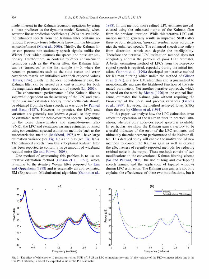
The enhancement performance of the Kalman filter issomewhat dependent on the accuracy of the LPC and exci-tation variance estimates. Ideally, these coefficients shouldbe obtained from the clean speech, as was done by Paliwaland Basu (1987). However, in practice, the LPCs andvariances are generally not known a priori, so they mustbe estimated from the noise-corrupted speech. Dependingon the noise characteristics and signal-to-noise ratio(SNR), the LPC and excitation variance estimates obtainedusing conventional spectral estimation methods (such as theautocorrelation method (Makhoul, 1975)) will have largeestimation variance (see Fig. 1(a)) and bias (see Fig. 1(b)).The enhanced speech from this suboptimal Kalman filterhas been reported to contain a large amount of widebandresidual noise (So and Paliwal, 2008).

One method of overcoming this problem is to use aniterative estimation method (Gibson et al., 1991), whichis similar to the iterative Wiener filter proposed by Limand Oppenheim (1978) and is essentially an approximatedEM (Expectation–Maximisation) algorithm (Gannot et al.,

0 0.5 1 1.5 2 2.5 335

40

45

50

55

60

65

70

75

80

Frequency (radians)

Pow

er (d

B)

(a)

Fig. 1. The effect of white noise (10 realisations) at an SNR of 15 dB on LPCtrue PSD estimate); and (b) the expected value of the PSD estimates.

1998). In this method, more refined LPC estimates are cal-culated using the enhanced output of the Kalman filterfrom the previous iteration. While this iterative LPC esti-mation method generally results in improved SNRs afterthree or four iterations, ‘musical’ residual noise accompa-nies the enhanced speech. The enhanced speech also suffersfrom distortion, which can degrade the intelligibility.Therefore the iterative LPC estimation method does notadequately address the problem of poor LPC estimates.A better estimation method of LPCs from the noise-cor-rupted speech is required, especially during the initial iter-ation. Gannot et al. (1998) developed an iterative methodfor Kalman filtering which unlike the method of Gibsonet al. (1991), is a true EM algorithm and is guaranteed tomonotonically increase the likelihood function of the esti-mated parameters. Yet another iterative approach, whichis based on the work by Mehra (1970) in the control liter-ature, estimates the Kalman gain without requiring theknowledge of the noise and process variances (Gabreaet al., 1999). However, the method achieved lower SNRsthan the one by Gibson et al. (1991).

In this paper, we analyse how the LPC estimation erroraffects the operation of the Kalman filter in practical situ-ations, whereby only noise-corrupted speech is available.In particular, we show the Kalman gain trajectory to bea useful indicator of the error of the LPC estimates andultimately the enhancement performance of the Kalman fil-ter. This detailed study will enable the motivation of newmethods to correct the Kalman gain as well as explainthe effectiveness of recently reported methods for reducingresidual noise in the output. These methods consist of twomodifications to the conventional Kalman filtering scheme(So and Paliwal, 2008): the use of long and overlappingspeech frames; and the application of tapered windowsduring LPC estimation. The Kalman gain analysis not onlyexplains the effectiveness of these two modifications, but it

0 0.5 1 1.5 2 2.5 335

40

45

50

55

60

65

70

75

80

Frequency (radians)

Pow

er (d

B)

(b)True PSDExpected value of PSD estimates

estimation showing: (a) the variance of the PSD estimates (thick line is the

S. So, K.K. Paliwal / Speech Communication 53 (2011) 355–378 357

also motivates further extensions to the method, namelythe use of Dolph–Chebychev windows with large sidelobeattenuation and iterative LPC estimation. The improve-ments provided by this method will be verified in objectiveand subjective speech enhancement experiments performedon the NOIZEUS speech corpus.

This paper is organised as follows. In Section 2, we givean introduction to speech enhancement using the Kalmanfilter as well as brief the reader on the mathematical nota-tion used in the recursive equations. We also attempt topinpoint the cause of suboptimality in the Kalman filterwhen only noise-corrupted speech is available, which willinclude a discussion on the importance of the Kalman gainand its time trajectories. In Section 3, we propose severalmodifications to the Kalman filter that effectively suppressthe influence of additive noise on the Kalman gain trajec-tory. The effectiveness of these modifications will be shownvia analysis of the Kalman gain trajectories, spectrograms,and objective measures such as SNR and segmental SNR.Section 4 describes the speech enhancement experimentsthat were performed on the NOIZEUS corpus (Hu andLoizou, 2006b) to verify the performance of the proposedKalman filter and compare it against other enhancementmethods, such as the iterative Kalman filter (Gibsonet al., 1991) and the MMSE–STSA method (Ephraimand Malah, 1984). White Gaussian noise and colouredcar noise at varying signal-to-noise ratios (SNRs) are inves-tigated. Two sets of objective scores are presented: (1)SNR, segmental SNR, and PESQ; and (2) composite mea-sures simulating the ITU-T P.835 methodology (Hu andLoizou, 2006a). Subjective preference scores from a blindAB listening test are also presented. Finally, we offer ourconcluding remarks in Section 5.

(observation)

excitation

noise−corrupted speech

white Gaussian noise

2. Speech enhancement using the Kalman filter

2.1. The Kalman recursion equations

If the clean speech is represented as x(n) and the noisesignal as v(n) (for n = 0, 1, . . .,N), then the noise-corruptedspeech y(n), which is the only observable signal in practice,is expressed as:

yðnÞ ¼ xðnÞ þ vðnÞ: ð1Þ

In the Kalman filter that is used for speech enhancement(Paliwal and Basu, 1987), v(n) is a zero-mean, white Gauss-ian noise that is uncorrelated with x(n).3 A pth order linearpredictor is used to model the speech signal:

xðnÞ ¼ �Xp

k¼1

akxðn� kÞ þ wðnÞ; ð2Þ

3 For the case where speech has been corrupted by coloured noise, anadditional linear predictor of order q is used to model the coloured noise,which augments the Kalman state vector to a size of p + q (Gibson et al.,1991).

where {ak; k = 1,2, . . . ,p} are the LPCs and w(n) is a whiteGaussian excitation with zero mean and a variance of r2

w.Fig. 2 shows a block diagram of the speech productionmodel and additive noise. Rewriting Eqs. (1) and (2) usingstate vector representation:

xðnÞ ¼ Axðn� 1Þ þ dwðnÞ; ð3ÞyðnÞ ¼ cT xðnÞ þ vðnÞ; ð4Þ

where x(n) = [x(n)x(n � 1) ,. . .,x(n � p + 1)]T is the ‘hidden’state vector, d = [10,. . ., 0]T and c = [10, . . ., 0]T are themeasurement vectors for the excitation noise and observa-tion, respectively. The linear prediction state transitionmatrix A is given by:

A ¼

�a1 �a2 . . . �ap�1 �ap

1 0 . . . 0 0

0 1 . . . 0 0

..

. ... . .

. ... ..

.

0 0 . . . 1 0

26666664

37777775: ð5Þ

The Kalman filter calculates xðnjnÞ, which is an unbiased,linear MMSE estimate of the state vector x(n), given thesamples of corrupted speech up to time n (i.e. y(1),y(2), . . .,y(n)), by using the following recursive equations:

xðnjn� 1Þ ¼ Axðn� 1jn� 1Þ; ð6ÞPðnjn� 1Þ ¼ APðn� 1jn� 1ÞAT þ r2

wddT ; ð7Þ

KðnÞ ¼ Pðnjn� 1Þc r2v þ cT Pðnjn� 1Þc

� ��1; ð8Þ

xðnjnÞ ¼ xðnjn� 1Þ þ KðnÞ½yðnÞ � cT xðnjn� 1Þ�; ð9ÞPðnjnÞ ¼ ½I� KðnÞcT �Pðnjn� 1Þ; ð10Þ

We briefly explain what each variable in the above recur-sive equations represents:

� xðnjn� 1Þ is the a priori estimate of the current state vec-tor at time n, given the observations up to n � 1;� r2

v is the variance of the corrupting noise v(n);� P(njn � 1) is the error covariance matrix of the a priori

estimate, xðnjn� 1Þ, i.e. E{e(njn � 1) eT(njn � 1)}, whereE{�} is the expectation operator and eðnjn� 1Þ ¼xðnÞ � xðnjn� 1Þ;� The expression yðnÞ � cT xðnjn� 1Þ in Eq. (9) is termed

the innovation, as it represents the information containedin the current observation y(n) that cannot be predictedby the dynamic model;

(vocal tract model)linear predictor

Fig. 2. Block diagram showing the speech production model (linearpredictor) and white Gaussian noise that is added to the speech.

Fig. 3. Block diagram of the Kalman filter. Bolded variables are vectors.

Enhanced speech

Kalman statevectors

Enhanced speech

Kalman statevectors

Fig. 4. Diagram showing the difference between the two types of Kalmanfilters (of state vector length of 3) described by Paliwal and Basu (1987):(a) In the zero-lag Kalman filter, the first component (shown as a shadedbox) of each estimated state vector is taken as the estimated speechsample; (b) In the fixed-lag Kalman filter, the last component (shown as ashaded box) of each estimated state vector is taken as the estimated speechsample.


� xðnjnÞ is the a posteriori estimate of x(n), given theobservations up to n, which consists of the a priori esti-mate xðnjn� 1Þ corrected with the innovation weightedby the Kalman gain K(n); and� P(n—n) is the error covariance matrix of the a posteriori

estimate.

The current estimated sample is then given byxðnÞ ¼ cT xðnjnÞ, which extracts the first component of theestimated state vector. Fig. 3 shows a block diagram ofthe Kalman filter.

During the operation of the Kalman filter, the noise-cor-rupted speech y(n) is windowed into short (e.g. 20 ms) andnon-overlapped frames, where the LPCs and excitationvariance r2

w are estimated. These LPCs remain constantduring the Kalman filtering of speech samples in the frame,while the Kalman parameters (such as Kalman gain K(n)and error covariance P(njn)) and state vector estimatexðnjnÞ are continually updated on a sample-by-samplebasis (regardless of which frame we are in).

2.2. Zero-lag and fixed-lag Kalman filters

Two types of Kalman filter were discussed by Paliwaland Basu (1987), which we will refer to in this paper asthe zero-lag and fixed-lag Kalman filter.4 These are shownin Fig. 4. In the zero-lag Kalman filter, the currentenhanced speech sample xðnÞ is formed by taking the firstcomponent of the estimated state vector xðnjnÞ. This com-ponent is calculated based on information from past andcurrent observations of the noise-corrupted speech as wellas past estimated speech samples.

For the fixed-lag Kalman filter (also referred to as thedelayed Kalman filter by Paliwal and Basu (1987)), the pastenhanced speech sample xðn� p þ 1Þ is formed by takingthe last component of the estimated state vector xðnjnÞ.In effect, this past speech sample is re-estimated using infor-mation that is based on:

4 Note that the term ‘lag’ refers to the delay caused by block-basedprocessing, rather than the computational delay.

� future noisy observations, i.e. {y(n � p + 2), y(n � p +3), . . .,y(n)}; and� future speech estimates, i.e. fxðn� p þ 2Þ; xðn� p þ 3Þ;

. . . ; xðn� 1Þg.

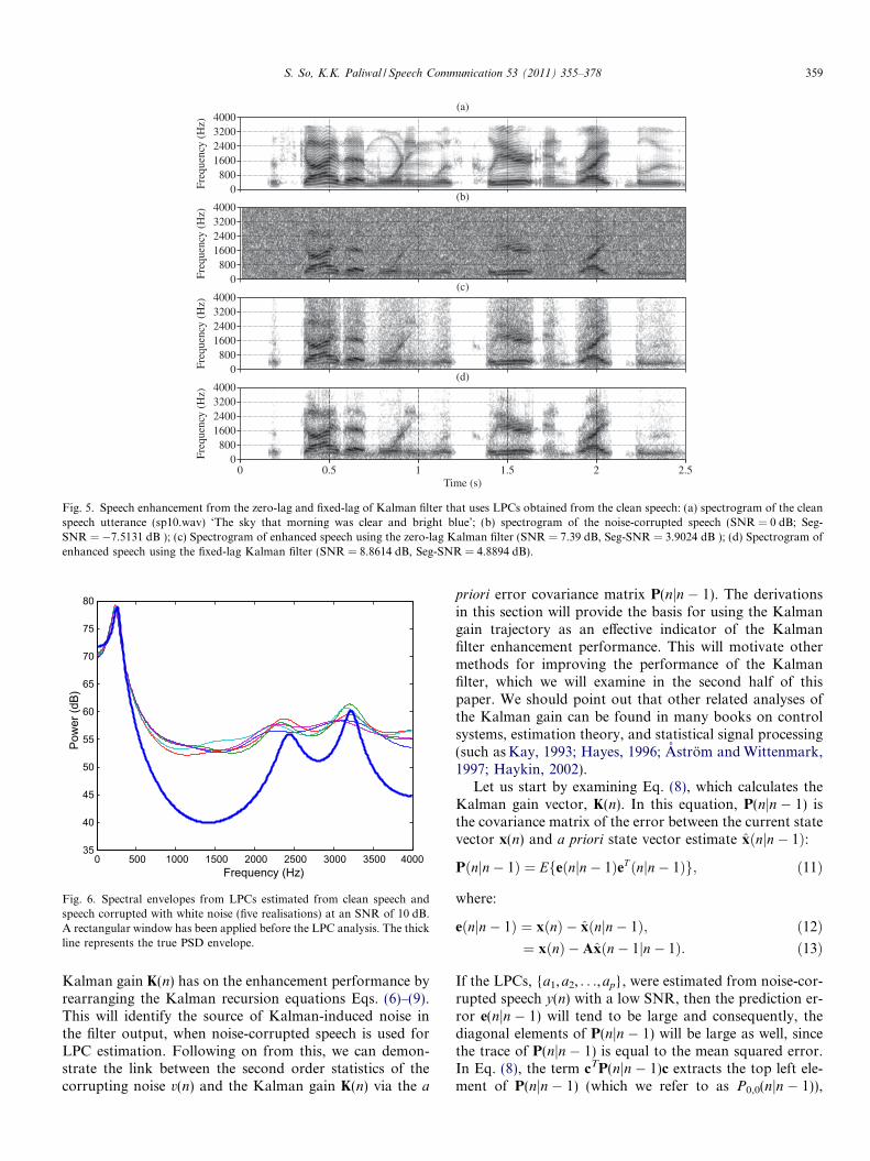
Therefore, the fixed-lag Kalman filter, which we willadopt in our study, can be viewed as a fixed-lag smoother,which was shown to give better enhancement than the zero-lag Kalman filter (Paliwal and Basu, 1987). Fig. 5 showsthe spectrograms of the clean, noisy, and enhanced speechfrom the zero-lag and fixed-lag Kalman filter. Note that theLPCs were estimated from the clean speech in this example,hence this can be viewed as the best case scenario for theKalman filter.

2.3. Using LPCs estimated from noise-corrupted speech in

the Kalman filter

In practice, the clean speech is not available and so theLPCs need to be estimated from the noise-corruptedspeech. Fig. 6 shows the effect of noise on the LPC esti-mates, where five realisations of white Gaussian noise havebeen added to a frame of speech at varying SNRs. TheLPCs were estimated using the autocorrelation method(Makhoul, 1975). It can be seen that the spectral tilt as wellas the sharpness and dynamic range of the two formantsabove 2 kHz have been reduced.

To understand the repercussions of inaccurate LPCs onthe Kalman filter, we will firstly examine the effect that the

0800

1600240032004000

Freq

uenc

y (H

z)

(a)

0800

1600240032004000

Freq

uenc

y (H

z)(b)

0800

1600240032004000

Freq

uenc

y (H

z)

(c)

0800

1600240032004000

(d)

Freq

uenc

y (H

z)

0 0.5 1 1.5 2 2.5Time (s)

Fig. 5. Speech enhancement from the zero-lag and fixed-lag of Kalman filter that uses LPCs obtained from the clean speech: (a) spectrogram of the cleanspeech utterance (sp10.wav) ‘The sky that morning was clear and bright blue’; (b) spectrogram of the noise-corrupted speech (SNR = 0 dB; Seg-SNR = �7.5131 dB ); (c) Spectrogram of enhanced speech using the zero-lag Kalman filter (SNR = 7.39 dB, Seg-SNR = 3.9024 dB ); (d) Spectrogram ofenhanced speech using the fixed-lag Kalman filter (SNR = 8.8614 dB, Seg-SNR = 4.8894 dB).

0 500 1000 1500 2000 2500 3000 3500 400035

40

45

50

55

60

65

70

75

80

Frequency (Hz)

Pow

er (d

B)

Fig. 6. Spectral envelopes from LPCs estimated from clean speech andspeech corrupted with white noise (five realisations) at an SNR of 10 dB.A rectangular window has been applied before the LPC analysis. The thickline represents the true PSD envelope.


Kalman gain K(n) has on the enhancement performance byrearranging the Kalman recursion equations Eqs. (6)–(9).This will identify the source of Kalman-induced noise inthe filter output, when noise-corrupted speech is used forLPC estimation. Following on from this, we can demon-strate the link between the second order statistics of thecorrupting noise v(n) and the Kalman gain K(n) via the a

priori error covariance matrix P(njn � 1). The derivationsin this section will provide the basis for using the Kalmangain trajectory as an effective indicator of the Kalmanfilter enhancement performance. This will motivate othermethods for improving the performance of the Kalmanfilter, which we will examine in the second half of thispaper. We should point out that other related analyses ofthe Kalman gain can be found in many books on controlsystems, estimation theory, and statistical signal processing(such as Kay, 1993; Hayes, 1996; Astrom and Wittenmark,1997; Haykin, 2002).

Let us start by examining Eq. (8), which calculates theKalman gain vector, K(n). In this equation, P(njn � 1) isthe covariance matrix of the error between the current statevector x(n) and a priori state vector estimate xðnjn� 1Þ:

Pðnjn� 1Þ ¼ Efeðnjn� 1ÞeT ðnjn� 1Þg; ð11Þ

where:

eðnjn� 1Þ ¼ xðnÞ � xðnjn� 1Þ; ð12Þ¼ xðnÞ � Axðn� 1jn� 1Þ: ð13Þ

If the LPCs, {a1,a2, . . .,ap}, were estimated from noise-cor-rupted speech y(n) with a low SNR, then the prediction er-ror e(njn � 1) will tend to be large and consequently, thediagonal elements of P(njn � 1) will be large as well, sincethe trace of P(njn � 1) is equal to the mean squared error.In Eq. (8), the term cTP(njn � 1)c extracts the top left ele-ment of P(njn � 1) (which we refer to as P0,0(njn � 1)),

0800

1600240032004000

Freq

uenc

y (H

z)

(a)

0800

1600240032004000

Freq

uenc

y (H

z)

(b)

00.20.40.60.8

1(c)

0800

1600240032004000

Freq

uenc

y (H

z)

(d)

00.20.40.60.8

1(e)

Time (s)0 2.5

0

4000

Freq

uenc

y (H

z)

0 0.5 1 1.5 2 2.50

8001600240032004000

(f)

Fig. 7. The influence of LPC estimates and Kalman gain on the enhancement performance of the Kalman filter: (a) spectrogram of the clean speechutterance (sp10.wav); (b) spectrogram of speech corrupted with white noise at SNR of 0 dB; (c) first component of Kalman gain, K0(n), when LPCs are

estimated from clean speech; (d) spectrogram of enhanced speech using Kalman filter of part (c); (e) plot of the first component of Kalman gain, K0(n),when LPCs are estimated from noise-corrupted speech; (f) spectrogram of enhanced speech using Kalman filter of part (e) (SNR = 4.293 dB, Seg-SNR = �3.194 dB).

5 This is the case for the zero-lag Kalman filter. The analysis of the fixed-lag Kalman filter is slightly more complicated due to the recursive natureof the state vector estimates. We assume here that the fixed-lag Kalmanfilter can do no worse than the zero-lag Kalman filter.


which is the predicted error variance of the first componentof xðnjn� 1Þ, while the term P(njn � 1)c takes the first col-umn of P(njn � 1) (which we refer to as P0(njn � 1)).

The first component of the Kalman gain vector (whichwe will refer to as K0(n)), can be expressed as (by rewritingEq. (8)):

K0ðnÞ ¼P 0;0ðnjn� 1Þ

r2v þ P 0;0ðnjn� 1Þ : ð14Þ

If the variance of the corrupting white noise r2v is close to

zero, then K0(n) will be close to one. If r2v is much larger

than the predicted error variance, then K0(n) will be closeto zero. We rearrange Eq. (9) to give the following form:

xðnjnÞ ¼ ½I� KðnÞcT �xðnjn� 1Þ þ KðnÞyðnÞ: ð15Þ

We can see in Eq. (15) that the Kalman gain acts as a reg-ulator, controlling the relative proportions of the noisyobservation and predicted state vector that are added to

give the a posteriori estimate xðnjnÞ. If we consider the firstcomponent5 of all vector quantities in Eq. (15), which wedenote with a subscript 0, we can further reduce it down to:

x0ðnjnÞ ¼ ½1� K0ðnÞ�x0ðnjn� 1Þ þ K0ðnÞyðnÞ ð16Þ¼ ½1� K0ðnÞ�x0ðnjn� 1Þ þ K0ðnÞxðnÞ þ K0ðnÞvðnÞ|fflfflfflfflfflffl{zfflfflfflfflfflffl}

residual noise

ð17ÞHere, we can see that if K0(n) is equal to one, then theenhanced speech sample would be comprised entirely ofthe observation y(n). In this case, the observation is deemedby the Kalman filter to be reliable since the corrupting noisevariance is zero. On the other hand, if the observations

0 20 40 60 80 100 120 140−0.02

−0.015

−0.01

−0.005

0

0.005

0.01

0.015

0.02

0.025

Frame number

Varia

nce

(a)

Variance of noisy signalVariance of predicted signal (inverted)Prediction error

0 20 40 60 80 100 120 140−0.02

−0.015

−0.01

−0.005

0

0.005

0.01

0.015

0.02

0.025

Frame number

Varia

nce

(b)


0 20 40 60 80 100 120 140−0.02

−0.015

−0.01

−0.005

0

0.005

0.01

0.015

0.02

0.025

Frame number

Varia

nce

(c)


Fig. 8. Comparing variances of noise-corrupted signal y(n), predicted signal (inverted), and prediction error for different SNRs: (a) 10 dB; (b) 0 dB;(c) �5 dB. Note that the thick red line is the summation of the other two.

6 Note that Eq. (18) is effectively calculating the error variance bysubtracting the predicted signal variance from the variance of the originalsignal. The summation operation is due to the negative sign conventionthat we have used for linear prediction.


have a low SNR, then K0(n) will approach zero, so the en-hanced speech sample would be comprised entirely of thepredicted component.

Fig. 7 shows the influence of the Kalman gain on theenhancement performance of the Kalman filter. We cansee in Fig. 7(c) and (d), where the LPCs have been esti-mated from the clean speech, that when K0(n) is close tozero, the output of the Kalman filter is free from noise(during silence periods). In the section of speech startingfrom 0.36 s, K0(n) rises to about 0.7, which suggests thatthe enhanced output consists of 70% of the noisy observa-tion. As can be observed in the enhanced output spectro-gram, this observation signal provides the long-termcorrelation information (i.e. fine structure) that cannot bepredicted by the low order linear predictor, accompaniedby some noise (represented by the last term in Eq. (17)),which we will refer to as the residual noise, since it is a frac-tion of the observation noise that is passed to the output.Therefore, the amount of residual noise that is present inthe enhanced speech is dependent on the value of K0(n).

If we look at Fig. 7(e) and (f), where the LPCs have beenestimated from the noise-corrupted speech, we notice that

on average, K0(n) is quite high (above 0.5) for the entireutterance. This means that the enhanced output is formedfrom 50% of the noise component v(n), which explainsthe presence of residual noise. As the variance of the noise,r2

v , is relatively stationary throughout the entire utterance,then based on Eq. (14), we may pinpoint the cause to largediagonal elements in P(njn � 1), or more specificallyP0,0(njn � 1). Correspondingly from Eq. (7), we attributethese large values to the variance of the model excitation,r2

w, which for the autocorrelation method is given by:

r2w ¼ Ryyð0Þ|fflffl{zfflffl}

signal variance

þXp

k¼1akRyyðkÞ|fflfflfflfflfflfflfflfflfflfflffl{zfflfflfflfflfflfflfflfflfflfflffl}

prediction variance

; ð18Þ

where Ryy(k) is the kth autocorrelation coefficient of the sig-nal y(n).6 Fig. 8 shows the variances of the noise-corruptedsignal (i.e. Ryy(0)), predicted signal (i.e.

Ppk¼1akRyyðkÞ), and


mean squared prediction error (i.e. r2w) for different SNRs.

We can see that as the SNR is lowered, the variance of thenoise-corrupted signal (thin green line) goes up due toincreasing levels of noise but the variance of the predictedsignal (dashed blue line) decreases. This results in a netincrease in the prediction error variance.

Assuming the clean speech and noise signals (x(n) andv(n), respectively) are zero-mean and uncorrelated, wecan write:

RyyðkÞ ¼ RxxðkÞ þ RvvðkÞ: ð19Þ

Hence we can rewrite Eq. (7) as:

Pðnjn� 1Þ ¼ APðn� 1jn� 1ÞAT þ Rxxð0Þ þXp

k¼1

akRxxðkÞ

þ Rvvð0Þ þXp

k¼1

akRvvðkÞ!

ddT : ð20Þ

We can see from Eq. (20) the presence of extra terms re-lated to the noise v(n) causes estimates of the a priori errorcovariance P(njn � 1) to be large, resulting in a higher-than-usual Kalman gain and hence more residual noise inthe output.

Since P0,0(njn � 1) has been offset by the extra termsrelated to the noise v(n), we may rewrite Eq. (14) (withr2

v ¼ Rvvð0Þ):

K0ðnÞ ¼r2

v þPp

k¼1akRvvðkÞ þ P c0;0ðnjn� 1Þ

2r2v þ

Ppk¼1akRvvðkÞ þ P c

0;0ðnjn� 1Þ ; ð21Þ

0800

1600240032004000

Freq

uenc

y (H

z)

0800

1600240032004000

Freq

uenc

y (H

z)

00.20.40.60.8

1

Ti0

0

4000

Freq

uenc

y (H

z)

0 0.5 10

8001600240032004000

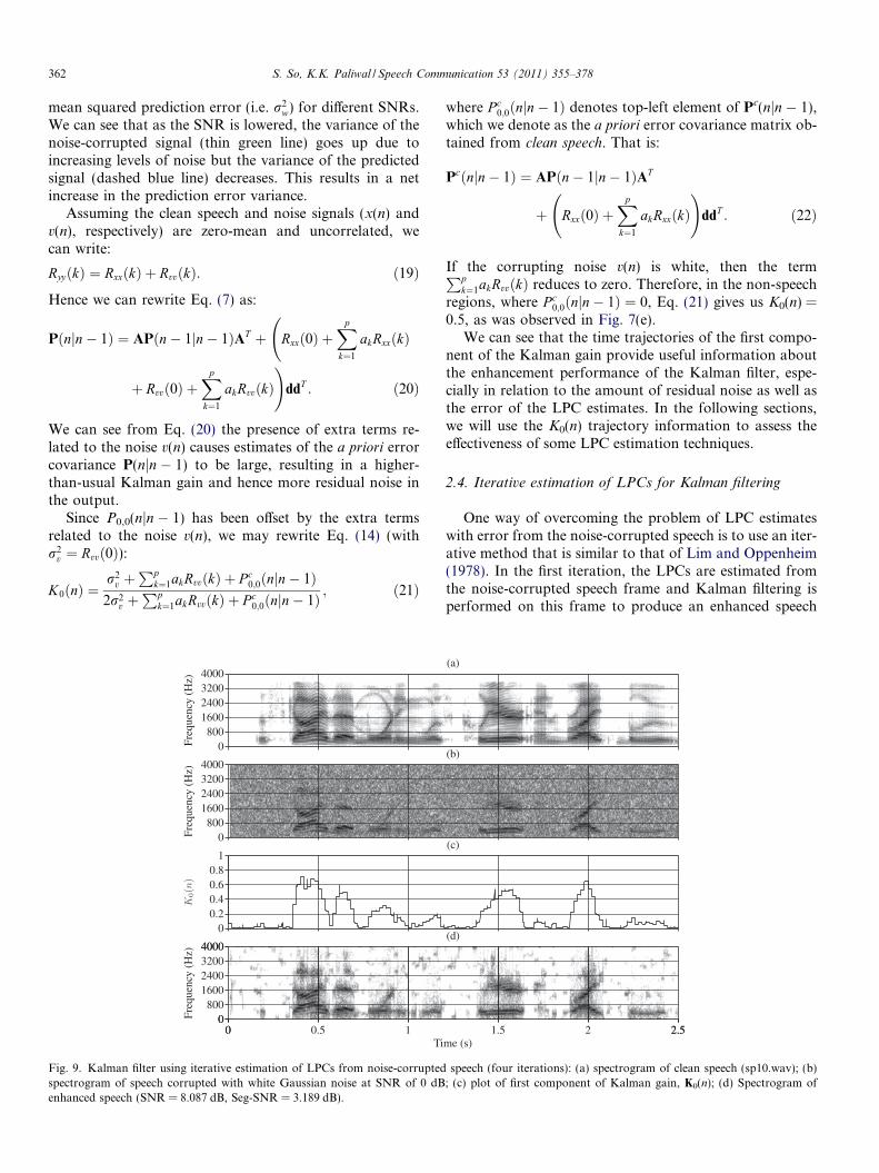
Fig. 9. Kalman filter using iterative estimation of LPCs from noise-corruptedspectrogram of speech corrupted with white Gaussian noise at SNR of 0 dBenhanced speech (SNR = 8.087 dB, Seg-SNR = 3.189 dB).

where P c0;0ðnjn� 1Þ denotes top-left element of Pc(njn � 1),

which we denote as the a priori error covariance matrix ob-tained from clean speech. That is:

Pcðnjn� 1Þ ¼ APðn� 1jn� 1ÞAT

þ Rxxð0Þ þXp

k¼1

akRxxðkÞ !

ddT : ð22Þ

If the corrupting noise v(n) is white, then the termPpk¼1akRvvðkÞ reduces to zero. Therefore, in the non-speech

regions, where P c0;0ðnjn� 1Þ ¼ 0, Eq. (21) gives us K0(n) =

0.5, as was observed in Fig. 7(e).We can see that the time trajectories of the first compo-

nent of the Kalman gain provide useful information aboutthe enhancement performance of the Kalman filter, espe-cially in relation to the amount of residual noise as well asthe error of the LPC estimates. In the following sections,we will use the K0(n) trajectory information to assess theeffectiveness of some LPC estimation techniques.

2.4. Iterative estimation of LPCs for Kalman filtering

One way of overcoming the problem of LPC estimateswith error from the noise-corrupted speech is to use an iter-ative method that is similar to that of Lim and Oppenheim(1978). In the first iteration, the LPCs are estimated fromthe noise-corrupted speech frame and Kalman filtering isperformed on this frame to produce an enhanced speech

(a)

(b)

(c)

me (s)2.51.5 2 2.5

(d)

speech (four iterations): (a) spectrogram of clean speech (sp10.wav); (b); (c) plot of first component of Kalman gain, K0(n); (d) Spectrogram of

0 20 40 60 80 100 120 140 1600

0.2

0.4

0.6

0.8

1

1.2

Time sample

w(n

)

(a)

−1.5 −1 −0.5 0 0.5 1 1.5−120

−100

−80

−60

−40

−20

0

Frequency (radians)

|W(f)

|2 (dB)

(b)

RectangularHammingDolph−Chebychev

Hamming windowRectangular window Dolph−Chebychev window

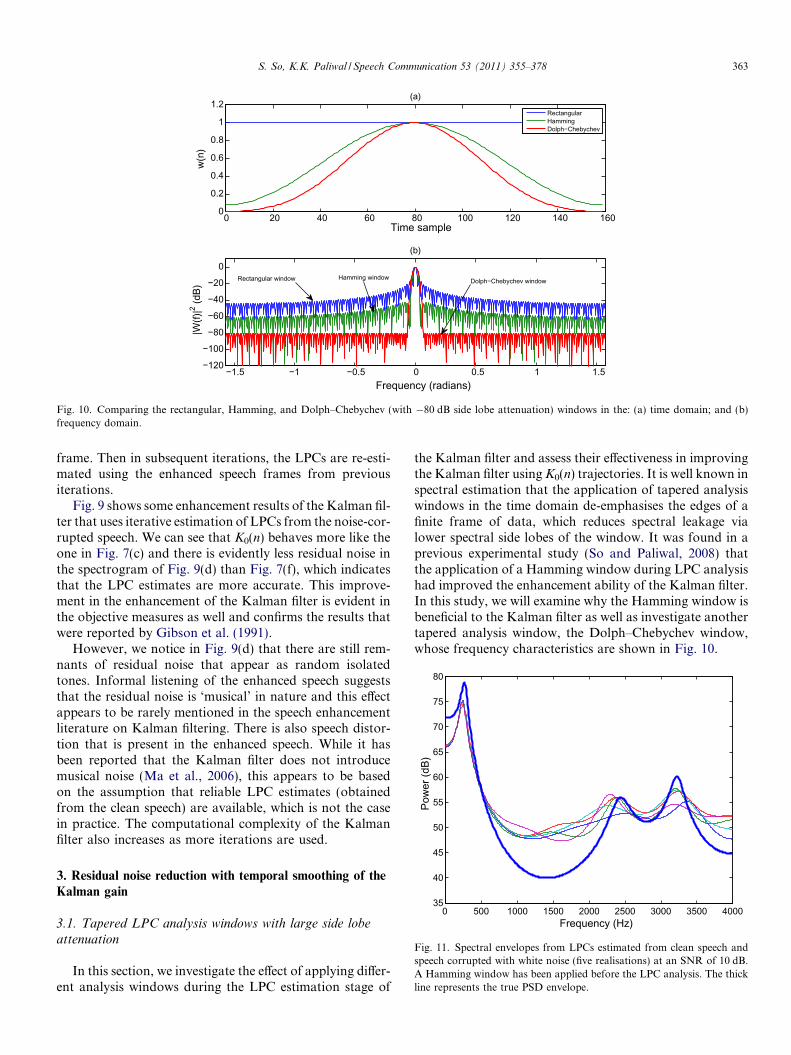
Fig. 10. Comparing the rectangular, Hamming, and Dolph–Chebychev (with �80 dB side lobe attenuation) windows in the: (a) time domain; and (b)frequency domain.

50

55

60

65

70

75

80

Pow

er (d

B)


frame. Then in subsequent iterations, the LPCs are re-esti-mated using the enhanced speech frames from previousiterations.

Fig. 9 shows some enhancement results of the Kalman fil-ter that uses iterative estimation of LPCs from the noise-cor-rupted speech. We can see that K0(n) behaves more like theone in Fig. 7(c) and there is evidently less residual noise inthe spectrogram of Fig. 9(d) than Fig. 7(f), which indicatesthat the LPC estimates are more accurate. This improve-ment in the enhancement of the Kalman filter is evident inthe objective measures as well and confirms the results thatwere reported by Gibson et al. (1991).

However, we notice in Fig. 9(d) that there are still rem-nants of residual noise that appear as random isolatedtones. Informal listening of the enhanced speech suggeststhat the residual noise is ‘musical’ in nature and this effectappears to be rarely mentioned in the speech enhancementliterature on Kalman filtering. There is also speech distor-tion that is present in the enhanced speech. While it hasbeen reported that the Kalman filter does not introducemusical noise (Ma et al., 2006), this appears to be basedon the assumption that reliable LPC estimates (obtainedfrom the clean speech) are available, which is not the casein practice. The computational complexity of the Kalmanfilter also increases as more iterations are used.

0 500 1000 1500 2000 2500 3000 3500 400035

40

45

Frequency (Hz)

Fig. 11. Spectral envelopes from LPCs estimated from clean speech andspeech corrupted with white noise (five realisations) at an SNR of 10 dB.A Hamming window has been applied before the LPC analysis. The thickline represents the true PSD envelope.

3. Residual noise reduction with temporal smoothing of the

Kalman gain

3.1. Tapered LPC analysis windows with large side lobe

attenuation

In this section, we investigate the effect of applying differ-ent analysis windows during the LPC estimation stage of

the Kalman filter and assess their effectiveness in improvingthe Kalman filter using K0(n) trajectories. It is well known inspectral estimation that the application of tapered analysiswindows in the time domain de-emphasises the edges of afinite frame of data, which reduces spectral leakage vialower spectral side lobes of the window. It was found in aprevious experimental study (So and Paliwal, 2008) thatthe application of a Hamming window during LPC analysishad improved the enhancement ability of the Kalman filter.In this study, we will examine why the Hamming window isbeneficial to the Kalman filter as well as investigate anothertapered analysis window, the Dolph–Chebychev window,whose frequency characteristics are shown in Fig. 10.

0 500 1000 1500 2000 2500 3000 3500 400035

40

45

50

55

60

65

70

75

80

Frequency (Hz)

Pow

er (d

B)

Fig. 12. Spectral envelopes from LPCs estimated from clean speech andspeech corrupted with white noise (five realisations) at an SNR of 10 dB.A Dolph–Chebychev window (with �200 dB side lobe attenuation) hasbeen applied before the LPC analysis. The thick line represents the truePSD estimate.

0 20 40 60 80 100 120 140 1600

0.20.40.60.8

1

Sample number

w(n

)

(a)

−1.5 −1 −0.5 0 0.5 1 1.5−250

−200

−150

−100

−50

0

Frequency (radians)

|W(f)

|2 (dB)

(b)

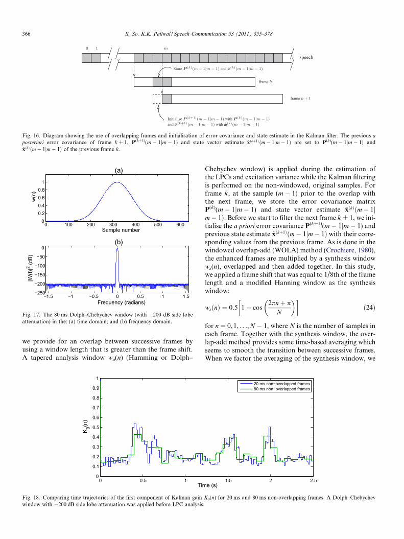
Fig. 13. The 20 ms Dolph–Chebychev window (with �200 dB side lobeattenuation) in the: (a) time domain; and (b) frequency domain.


Let us examine the effect of applying the Hamming win-dow on the spectral envelope of speech that has been cor-rupted by white noise. The non-iterative fixed-lagKalman filter was used in the experiments that are reportedin this section. Fig. 11 shows the spectral envelope fromLPCs that have been estimated from clean and five realisa-tions of noisy speech, where a Hamming window is appliedduring the LPC analysis. Comparing this with Fig. 6, wecan see that the spectral envelopes have lower power, whichsuggests a reduction in the excitation variance r2

w. Also, thedynamic range of the two formants has improved slightlywith lower spectral valleys. This indicates that the taperedanalysis window has an impact on LPC estimation in thepresence of noise or more specifically, the mean squaredprediction error, P0,0(njn � 1).

In order to test this theory further, we investigated theDolph–Chebychev window, whose side lobe attenuationcan be adjusted. This window, as shown in Fig. 13, wasdesigned to have a very large side lobe attenuation(�200 dB). Fig. 12 shows the spectral envelopes fromLPCs, where the Dolph–Chebychev window has beenapplied before LPC analysis. We can see that for eachrealisation, the formants appear to be sharper and moreresolvable than either the Hamming or rectangular win-dow. In particular, the spectral valleys are the lowest,which in effect also enhances the formants. We should notethat the variance of the spectral envelope estimates appearsto have increased with the tapered windows.

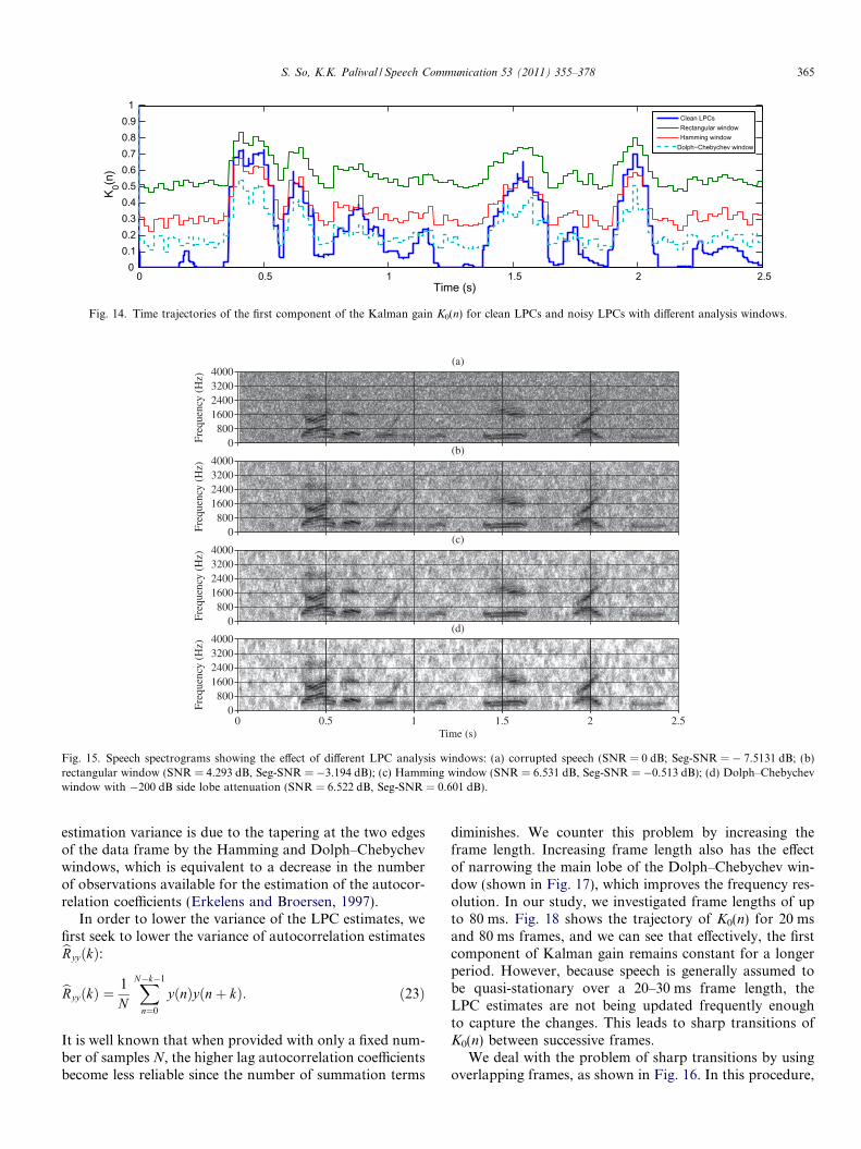
These results are consistent with those reported byErkelens and Broersen (1997), where tapered analysiswindows were shown to reduce the bias in the excitationor residual variance of the autocorrelation method. Thebenefit that this result brings to the Kalman filter is madeobvious when we consider the effect of a lower P0,0(njn � 1)in Eq. (21). The reduction of excitation variance via the

application of a tapered window counteracts the bias intro-duced by the corrupting noise (i.e. r2

v), which leads to lowerKalman gain trajectories.

Fig. 14 shows the time trajectories of K0(n) for the differ-ent analysis windows. Also shown in this plot is the K0(n)when LPCs are estimated from clean speech, which servesas the ‘best case scenario’. Recall that K0(n) gives the rela-tive proportion of the observation signal y(n) and we haveseen previously that it tends to be high in the voiced speechregions, since they contain long-term correlation informa-tion. When using the rectangular window for estimatingLPCs from noise-corrupted speech, K0(n) is high in theregions where there is very little speech and this results ina large amount of residual noise. We can see in Fig. 14 thatthe tapered analysis windows (Hamming and Dolph–Chebychev) result in lower K0(n) values than the rectangu-lar window and therefore we expect a reduced level ofresidual noise. We can see in Fig. 15(d) that there is lessresidual noise in the Dolph–Chebychev window case. How-ever, we can also see that the K0(n) for the Dolph–Cheby-chev window is lower than the K0(n) of the clean LPC casein the voiced speech regions, hence we expect enhancedspeech to have diminished fine structure. In terms of objec-tive measures, the tapered windows give higher SNRs andsegmental SNRs than the rectangular window.

3.2. Using long and overlapping speech frames for temporalsmoothing

It can be seen in Fig. 14 that K0(n) appears to fluctuateover time. As K0(n) also represents the proportion of noisev(n) that is added to the enhanced speech (see the last termof Eq. (17)), these fluctuations result in a non-stationaryresidual noise that may be annoying to listeners. Lookingat Eq. (8) and assuming that the variance of the noise r2

v

remains relatively constant, we may attribute these fluctua-tions to high variance LPC estimates. The increased LPC

0 0.5 1 1.5 2 2.50

0.10.20.30.40.50.60.70.80.9

1K 0(n

)

Time (s)

Clean LPCsRectangular windowHamming window

Dolph−Chebychev window

Fig. 14. Time trajectories of the first component of the Kalman gain K0(n) for clean LPCs and noisy LPCs with different analysis windows.

0800

1600240032004000

Freq

uenc

y (H

z)

(a)

0800

1600240032004000

Freq

uenc

y (H

z)

(b)

0800

1600240032004000

Freq

uenc

y (H

z)

(c)

0800

1600240032004000

0 0.5 1 1.5 2 2.5Time (s)

Freq

uenc

y (H

z)

(d)

Fig. 15. Speech spectrograms showing the effect of different LPC analysis windows: (a) corrupted speech (SNR = 0 dB; Seg-SNR = � 7.5131 dB; (b)rectangular window (SNR = 4.293 dB, Seg-SNR = �3.194 dB); (c) Hamming window (SNR = 6.531 dB, Seg-SNR = �0.513 dB); (d) Dolph–Chebychevwindow with �200 dB side lobe attenuation (SNR = 6.522 dB, Seg-SNR = 0.601 dB).


estimation variance is due to the tapering at the two edgesof the data frame by the Hamming and Dolph–Chebychevwindows, which is equivalent to a decrease in the numberof observations available for the estimation of the autocor-relation coefficients (Erkelens and Broersen, 1997).

In order to lower the variance of the LPC estimates, wefirst seek to lower the variance of autocorrelation estimatesbRyyðkÞ:

bRyyðkÞ ¼1

N

XN�k�1

n¼0

yðnÞyðnþ kÞ: ð23Þ

It is well known that when provided with only a fixed num-ber of samples N, the higher lag autocorrelation coefficientsbecome less reliable since the number of summation terms

diminishes. We counter this problem by increasing theframe length. Increasing frame length also has the effectof narrowing the main lobe of the Dolph–Chebychev win-dow (shown in Fig. 17), which improves the frequency res-olution. In our study, we investigated frame lengths of upto 80 ms. Fig. 18 shows the trajectory of K0(n) for 20 msand 80 ms frames, and we can see that effectively, the firstcomponent of Kalman gain remains constant for a longerperiod. However, because speech is generally assumed tobe quasi-stationary over a 20–30 ms frame length, theLPC estimates are not being updated frequently enoughto capture the changes. This leads to sharp transitions ofK0(n) between successive frames.

We deal with the problem of sharp transitions by usingoverlapping frames, as shown in Fig. 16. In this procedure,

Fig. 16. Diagram showing the use of overlapping frames and initialisation of error covariance and state estimate in the Kalman filter. The previous a

posteriori error covariance of frame k + 1, P(k+1)(m � 1jm � 1) and state vector estimate xðkþ1Þðm� 1jm� 1Þ are set to P(k)(m � 1jm � 1) andxðkÞðm� 1jm� 1Þ of the previous frame k.

0 100 200 300 400 500 6000

0.20.40.60.8

1

Sample number

w(n

)

(a)

−1.5 −1 −0.5 0 0.5 1 1.5−250

−200

−150

−100

−50

0

Frequency (radians)

|W(f)

|2 (dB)

(b)

Fig. 17. The 80 ms Dolph–Chebychev window (with �200 dB side lobeattenuation) in the: (a) time domain; and (b) frequency domain.


we provide for an overlap between successive frames byusing a window length that is greater than the frame shift.A tapered analysis window wa(n) (Hamming or Dolph–

0 0.5 10

0.1

0.2

0.3

0.4

0.5

0.6

0.7

0.8

0.9

1

Tim

K 0(n)

Fig. 18. Comparing time trajectories of the first component of Kalman gainwindow with �200 dB side lobe attenuation was applied before LPC analysis.

Chebychev window) is applied during the estimation ofthe LPCs and excitation variance while the Kalman filteringis performed on the non-windowed, original samples. Forframe k, at the sample (m � 1) prior to the overlap withthe next frame, we store the error covariance matrixP(k)(m � 1jm � 1) and state vector estimate xðkÞðm� 1jm� 1Þ. Before we start to filter the next frame k + 1, we ini-tialise the a priori error covariance P(k+1)(m � 1jm � 1) andprevious state estimate xðkþ1Þðm� 1jm� 1Þ with their corre-sponding values from the previous frame. As is done in thewindowed overlap-add (WOLA) method (Crochiere, 1980),the enhanced frames are multiplied by a synthesis windowws(n), overlapped and then added together. In this study,we applied a frame shift that was equal to 1/8th of the framelength and a modified Hanning window as the synthesiswindow:

wsðnÞ ¼ 0:5 1� cos2pnþ p

N

� �� ð24Þ

for n = 0,1, . . .,N � 1, where N is the number of samples ineach frame. Together with the synthesis window, the over-lap-add method provides some time-based averaging whichseems to smooth the transition between successive frames.When we factor the averaging of the synthesis window, we

1.5 2 2.5e (s)

20 ms non−overlapped frames80 ms non−overlapped frames

K0(n) for 20 ms and 80 ms non-overlapping frames. A Dolph–Chebychev

0 0.5 1 1.5 2 2.50

0.1

0.2

0.3

0.4

0.5

0.6

0.7

0.8

0.9

1

Time (s)

K 0(n)

20 ms non−overlapped frames80 ms overlapped frames

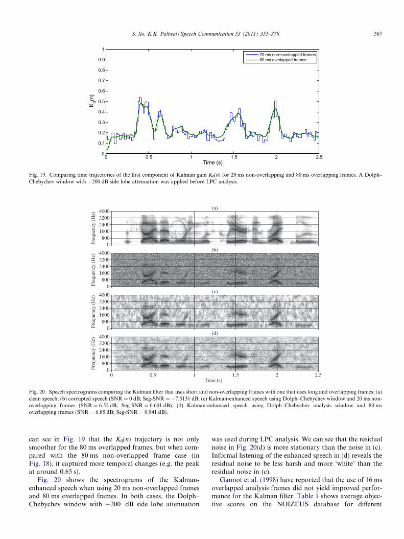
Fig. 19. Comparing time trajectories of the first component of Kalman gain K0(n) for 20 ms non-overlapping and 80 ms overlapping frames. A Dolph–Chebychev window with �200 dB side lobe attenuation was applied before LPC analysis.

0800

1600240032004000

Freq

uenc

y (H

z)

(a)

0800

1600240032004000

Freq

uenc

y (H

z)

(b)

0800

1600240032004000

(c)

Freq

uenc

y (H

z)

0800

1600240032004000

0 0.5 1 1.5 2 2.5Time (s)

Freq

uenc

y (H

z)

(d)

Fig. 20. Speech spectrograms comparing the Kalman filter that uses short and non-overlapping frames with one that uses long and overlapping frames: (a)clean speech; (b) corrupted speech (SNR = 0 dB; Seg-SNR = �7.5131 dB; (c) Kalman-enhanced speech using Dolph–Chebychev window and 20 ms non-overlapping frames (SNR = 6.52 dB; Seg-SNR = 0.601 dB); (d) Kalman-enhanced speech using Dolph–Chebychev analysis window and 80 msoverlapping frames (SNR = 6.85 dB; Seg-SNR = 0.941 dB).


can see in Fig. 19 that the K0(n) trajectory is not onlysmoother for the 80 ms overlapped frames, but when com-pared with the 80 ms non-overlapped frame case (inFig. 18), it captured more temporal changes (e.g. the peakat around 0.65 s).

Fig. 20 shows the spectrograms of the Kalman-enhanced speech when using 20 ms non-overlapped framesand 80 ms overlapped frames. In both cases, the Dolph–Chebychev window with �200 dB side lobe attenuation

was used during LPC analysis. We can see that the residualnoise in Fig. 20(d) is more stationary than the noise in (c).Informal listening of the enhanced speech in (d) reveals theresidual noise to be less harsh and more ‘white’ than theresidual noise in (c).

Gannot et al. (1998) have reported that the use of 16 msoverlapped analysis frames did not yield improved perfor-mance for the Kalman filter. Table 1 shows average objec-tive scores on the NOIZEUS database for different

Table 1Average objective scores on the NOIZEUS database (white Gaussiannoise with SNR of 0 dB) comparing the non-overlapped and overlappingmodes (frame update of 1/8th the frame duration) of the Kalman filter.(Note that ‘rect’ and ‘D–C’ stands for rectangular and Dolph–Chebychevwindows, respectively.)

Method (ms) SNR (dB) Seg-SNR (dB) PESQ

20, no overlap, rect window 4.461 �3.868 1.73920, with overlap, rect window 4.50 �3.859 1.74

80, no overlap, rect window 4.539 �3.853 1.73380, with overlap, rect window 4.66 �3.811 1.745

20, no overlap, D–C window 6.756 �0.011 1.82920, with overlap, D–C window 7.052 0.14 1.866

80, no overlap, D–C window 6.239 0.01 1.80880, with overlap, D–C window 7.074 0.381 1.908


configurations of the Kalman filter. We can see that when arectangular analysis window is applied, overlapping theframes did not produce any appreciable improvement, aswas observed by Gannot et al. (1998). However, whenusing long frames with a tapered analysis window, wecan see that overlapping the frames had yielded improvedperformance. This may be explained by the fact that sym-metric tapered windows emphasise only the centre of aframe, so overlapping ensures all samples receive the sameweighting when used for LPC estimation in successiveframes. In addition to this, overlapping long framesensures more frequent updates, which is important fornon-stationary speech signals.

0800

1600240032004000

Freq

uenc

y (H

z)

0800

1600240032004000

Freq

uenc

y (H

z)

0800

1600240032004000

Freq

uenc

y (H

z)

0 0.5 10

8001600240032004000

Freq

uenc

y (H

z)

Tim

Fig. 21. Speech spectrograms of the iterative Kalman filter (two iterations) thspeech; (b) corrupted speech (SNR = 0 dB; Seg-SNR = �7.5131 dB; (c) enhanwindow (SNR = 8.199 dB; Seg-SNR = 2.516 dB); (d) Kalman-enhanced speec(SNR = 7.67 dB; Seg-SNR = 3.25 dB).

3.3. Iterative LPC estimation with tapered analysis windows

and long overlapping frames

In this section, we investigate the use of long and over-lapping tapered windows for LPC analysis in the iterativeKalman filter. The problem with the iterative Kalman filterof Gibson et al. (1991) is that it uses LPCs derived from thenoise-corrupted speech to be used in the initialisation stage.We have observed that the non-iterative Kalman filter doesnot do such a good job at enhancing the speech (see Fig. 7),so further iterations are needed to obtain better enhance-ment. Our aim is to use the methods that we have discussedpreviously to initialise the iterative LPC estimation, so thatless iterations are required. Specifically, we use 80 ms over-lapping frames in all iterations. The tapered analysis win-dow is used in the LPC analysis of the initialisation stageonly, while the rectangular window is used in subsequentiterations.

Fig. 21 compares the spectrograms of the enhancedspeech using the Hamming and Dolph–Chebychev win-dows, where only two iterations have been performed.We can see that the residual noise in Fig. 21(d) has beenreduced when comparing with the spectrograms ofFig. 20(d). When comparing the spectrograms of usingthe Hamming window (Fig. 21(c)) with Dolph–Chebychev(Fig. 21(d)), the level of residual noise is higher in the for-mer. This is better indicated in Fig. 22, where we can seeK0(n) is always lower in the non-speech regions for theDolph–Chebychev window. Both tapered windows can be

(a)

(b)

(c)

1.5 2 2.5

(d)

e (s)

at uses 80 ms overlapping frames and tapered analysis window: (a) cleanced speech from iterative Kalman filter with 80 ms overlapping Hammingh using Dolph–Chebychev analysis window and 80 ms overlapping frames

0 0.5 1 1.5 2 2.50

0.1

0.2

0.3

0.4

0.5

0.6

0.7

0.8

0.9

1

Time (s)

K 0(n)

Hamming windowDolph−Chebychev windowRectangular windowClean LPC

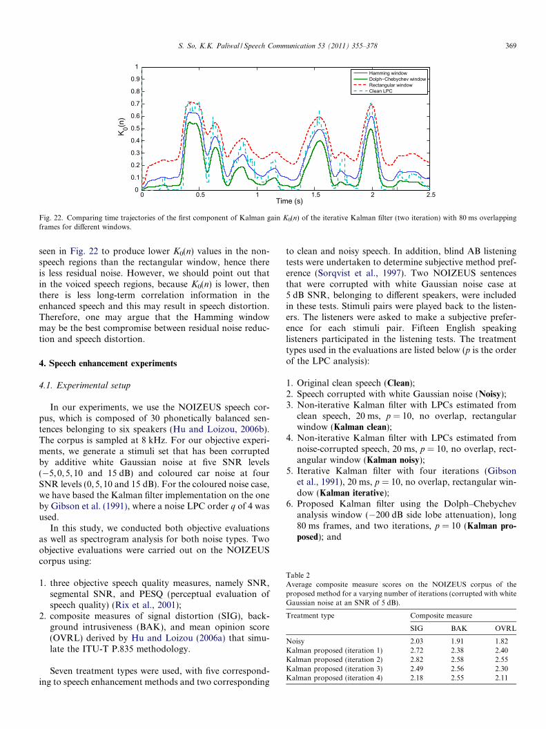
Fig. 22. Comparing time trajectories of the first component of Kalman gain K0(n) of the iterative Kalman filter (two iteration) with 80 ms overlappingframes for different windows.


seen in Fig. 22 to produce lower K0(n) values in the non-speech regions than the rectangular window, hence thereis less residual noise. However, we should point out thatin the voiced speech regions, because K0(n) is lower, thenthere is less long-term correlation information in theenhanced speech and this may result in speech distortion.Therefore, one may argue that the Hamming windowmay be the best compromise between residual noise reduc-tion and speech distortion.

Table 2Average composite measure scores on the NOIZEUS corpus of theproposed method for a varying number of iterations (corrupted with whiteGaussian noise at an SNR of 5 dB).

Treatment type Composite measure

SIG BAK OVRL

Noisy 2.03 1.91 1.82Kalman proposed (iteration 1) 2.72 2.38 2.40Kalman proposed (iteration 2) 2.82 2.58 2.55Kalman proposed (iteration 3) 2.49 2.56 2.30Kalman proposed (iteration 4) 2.18 2.55 2.11

4. Speech enhancement experiments

4.1. Experimental setup

In our experiments, we use the NOIZEUS speech cor-pus, which is composed of 30 phonetically balanced sen-tences belonging to six speakers (Hu and Loizou, 2006b).The corpus is sampled at 8 kHz. For our objective experi-ments, we generate a stimuli set that has been corruptedby additive white Gaussian noise at five SNR levels(�5,0,5,10 and 15 dB) and coloured car noise at fourSNR levels (0, 5,10 and 15 dB). For the coloured noise case,we have based the Kalman filter implementation on the oneby Gibson et al. (1991), where a noise LPC order q of 4 wasused.

In this study, we conducted both objective evaluationsas well as spectrogram analysis for both noise types. Twoobjective evaluations were carried out on the NOIZEUScorpus using:

1. three objective speech quality measures, namely SNR,segmental SNR, and PESQ (perceptual evaluation ofspeech quality) (Rix et al., 2001);

2. composite measures of signal distortion (SIG), back-ground intrusiveness (BAK), and mean opinion score(OVRL) derived by Hu and Loizou (2006a) that simu-late the ITU-T P.835 methodology.

Seven treatment types were used, with five correspond-ing to speech enhancement methods and two corresponding

to clean and noisy speech. In addition, blind AB listeningtests were undertaken to determine subjective method pref-erence (Sorqvist et al., 1997). Two NOIZEUS sentencesthat were corrupted with white Gaussian noise case at5 dB SNR, belonging to different speakers, were includedin these tests. Stimuli pairs were played back to the listen-ers. The listeners were asked to make a subjective prefer-ence for each stimuli pair. Fifteen English speakinglisteners participated in the listening tests. The treatmenttypes used in the evaluations are listed below (p is the orderof the LPC analysis):

1. Original clean speech (Clean);2. Speech corrupted with white Gaussian noise (Noisy);3. Non-iterative Kalman filter with LPCs estimated from

clean speech, 20 ms, p = 10, no overlap, rectangularwindow (Kalman clean);

4. Non-iterative Kalman filter with LPCs estimated fromnoise-corrupted speech, 20 ms, p = 10, no overlap, rect-angular window (Kalman noisy);

5. Iterative Kalman filter with four iterations (Gibsonet al., 1991), 20 ms, p = 10, no overlap, rectangular win-dow (Kalman iterative);

6. Proposed Kalman filter using the Dolph–Chebychevanalysis window (�200 dB side lobe attenuation), long80 ms frames, and two iterations, p = 10 (Kalman pro-

posed); and

Table 3Average objective scores on the NOIZEUS corpus of the proposedmethod as well as the non-iterative and iterative Kalman filter after two,three, and four iterations (corrupted with white Gaussian noise at an SNRof 5 dB).

Treatment type Objective measure

SNR (dB) SegSNR (dB) PESQ

Noisy 5.00 �3.31 1.82Kalman noisy 9.03 0.70 2.06Kalman iterative (iteration 2) 11.19 3.48 2.29Kalman iterative (iteration 3) 11.82 5.19 2.40Kalman iterative (iteration 4) 11.84 5.84 2.36Kalman proposed (iteration 2) 11.32 5.64 2.50


7. MMSE–STSA method (Ephraim and Malah, 1984)(MMSE).

−5 0 5 10 15−10

−5

0

5

10

15

20

Input SNR (dB)

Enha

nced

SN

R (d

B)

(a)

Kalman cleanKalman noisyKalman iterativeKalman proposedMMSENo enhancement

−5 0 51

1.5

2

2.5

3

3.5

Input S

PESQ

(c

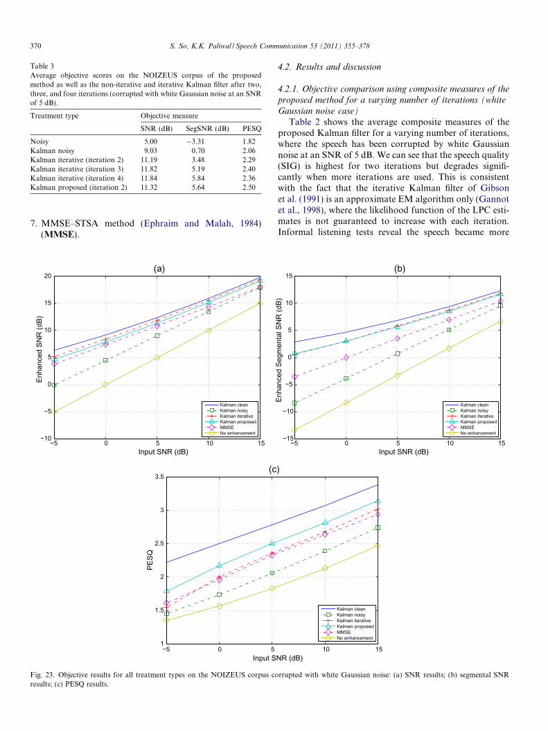
Fig. 23. Objective results for all treatment types on the NOIZEUS corpus coresults; (c) PESQ results.

4.2. Results and discussion

4.2.1. Objective comparison using composite measures of the

proposed method for a varying number of iterations (white

Gaussian noise case)

Table 2 shows the average composite measures of theproposed Kalman filter for a varying number of iterations,where the speech has been corrupted by white Gaussiannoise at an SNR of 5 dB. We can see that the speech quality(SIG) is highest for two iterations but degrades signifi-cantly when more iterations are used. This is consistentwith the fact that the iterative Kalman filter of Gibsonet al. (1991) is an approximate EM algorithm only (Gannotet al., 1998), where the likelihood function of the LPC esti-mates is not guaranteed to increase with each iteration.Informal listening tests reveal the speech became more

−5 0 5 10 15−15

−10

−5

0

5

10

15

Input SNR (dB)

Enha

nced

Seg

men

tal S

NR

(dB)

(b)


10 15NR (dB)

)


rrupted with white Gaussian noise: (a) SNR results; (b) segmental SNR

0800

1600240032004000

Freq

uenc

y (H

z)

(a)

0800

1600240032004000 (b)

Freq

uenc

y (H

z)

0800

1600240032004000

Freq

uenc

y (H

z)

(c)

0800

1600240032004000

Freq

uenc

y (H

z)

(d)

0800

1600240032004000

Freq

uenc

y (H

z)

(e)

0800

1600240032004000

Freq

uenc

y (H

z)

(f)

Time (s)0 2.5

0

4000

Freq

uenc

y (H

z)

0 0.5 1 1.5 2 2.50

8001600240032004000

(g)

Fig. 24. Spectrograms of all treatment types on the NOIZEUS corpus corrupted with white Gaussian noise at an SNR of 5 dB: (a) clean speech (sp10.wav)‘The sky that morning was clear and bright blue’; (b) noise-corrupted speech; (c) Kalman noisy; (d) Kalman iterative; (e) MMSE–STSA; (f) Kalman clean;(g) Kalman proposed.


and more suppressed in subsequent iterations. On the otherhand, the residual noise intrusiveness (BAK) score rosesharply when going to the second iteration but thenremained relatively constant in subsequent iterations.

4.2.2. Objective comparison using SNR, segmental SNR and

PESQ with the iterative Kalman filter (white Gaussian noise

case)

Table 3 shows the objective results of the proposed Kal-man filter as well as the non-iterative and iterative Kalmanfilter after a varying number of iterations for 5 dB of whiteGaussian noise. We can see that large improvements areobtained by using iterative estimation of the LPCs, asnoted in Gibson et al. (1991). The proposed Kalman filter,which uses effectively two iterations only, has achieved sim-

ilar SNR and segmental SNR scores as the four-iterationKalman filter. However, in terms of PESQ, the proposedKalman filter outperforms the iterative Kalman filter whileusing less iterations and hence, less computations.


PESQ with other enhancement methods (white Gaussian

noise case)

Fig. 23 shows the average objective scores for each ofthe different treatment types for the white Gaussian noisecase. We can see that the proposed method is competitivewith the iterative Kalman filter in terms of SNR and seg-mental SNR (Fig. 23(a) and (b)), despite the former requir-ing only half the number of iterations as the latter, whileoutperforming the other treatment types except for the

Table 4Average composite measure scores on the NOIZEUS corpus corruptedwith white Gaussian noise at an SNR of 5 dB.


SIG BAK OVRL

Noisy 2.03 1.91 1.82Kalman clean 3.72 2.94 3.18Kalman noisy 2.39 2.16 2.11Kalman iterative 2.41 2.44 2.25Kalman proposed 2.82 2.58 2.55MMSE 2.83 2.45 2.49


Kalman filter that uses clean-speech-derived LPCs. Interms of the PESQ score (Fig. 23(c)), it can be seen thatthe proposed Kalman filter, which uses a Dolph–Cheby-chev window with large side lobe attenuation and long80 ms frame lengths, outperforms all other enhancement

0 5 10 15−5

0

5

10

15

20

Input SNR (dB)

Enha

nced

SN

R (d

B)

(a)


0 51.6

1.8

2

2.2

2.4

2.6

2.8

3

3.2

Input SN

PESQ

(c)

Fig. 25. Objective results for all treatment types on the NOIZEUS corpus corru(c) PESQ results.

methods except for the Kalman filter that uses clean-speech-derived LPCs.

Fig. 24 shows the spectrograms of all the treatmenttypes. From these, we can see a large amount of residualnoise in the Kalman noisy case. This observation is consis-tent with our earlier analysis of the Kalman gain, where alarge value resulted in the passing through of noise frominput to output. The residual noise in Kalman-iterative(Fig. 24(d)) is much less, owing to better estimates of theLPCs. However, the residual noise appears to be musicalin nature and this was confirmed in informal listening tests.The speech was also quite distorted. In the output from theMMSE–STSA method (Fig. 24(e)), there is a high degree ofstructured residual noise that spans temporally. We can seethat enhanced speech from the proposed Kalman filter(Fig. 24(g)) has low residual noise. However, when com-pared with the original clean speech, there appears to be

0 5 10 15−10

−5

0

5

10

15

Input SNR (dB)

Enha

nced

Seg

men

tal S

NR

(dB)

(b)


10 15R (dB)


pted with car noise (coloured): (a) SNR results; (b) segmental SNR results;

0800

1600240032004000

Freq

uenc

y (H

z)

(a)

0800

1600240032004000

(b)

0800

1600240032004000

(c)

Freq

uenc

y (H

z)Fr

eque

ncy

(Hz)

0800

1600240032004000

Freq

uenc

y (H

z)

(d)

0800

1600240032004000

Freq

uenc

y (H

z)

(e)

0800

1600240032004000

Freq

uenc

y (H

z)

(f)

0 0.5 1 1.5 2 2.5Time (s)

0800

1600240032004000

Freq

uenc

y (H

z)

(g)

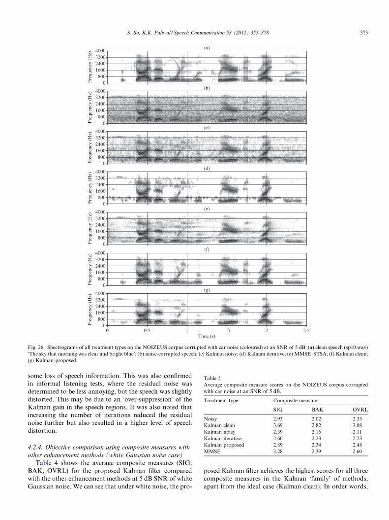
Fig. 26. Spectrograms of all treatment types on the NOIZEUS corpus corrupted with car noise (coloured) at an SNR of 5 dB: (a) clean speech (sp10.wav)‘The sky that morning was clear and bright blue’; (b) noise-corrupted speech; (c) Kalman noisy; (d) Kalman iterative; (e) MMSE–STSA; (f) Kalman clean;(g) Kalman proposed.

Table 5Average composite measure scores on the NOIZEUS corpus corruptedwith car noise at an SNR of 5 dB.


SIG BAK OVRL

Noisy 2.93 2.02 2.33Kalman clean 3.69 2.82 3.08Kalman noisy 2.39 2.16 2.11Kalman iterative 2.60 2.23 2.23Kalman proposed 2.89 2.34 2.48MMSE 3.28 2.39 2.60


some loss of speech information. This was also confirmedin informal listening tests, where the residual noise wasdetermined to be less annoying, but the speech was slightlydistorted. This may be due to an ‘over-suppression’ of theKalman gain in the speech regions. It was also noted thatincreasing the number of iterations reduced the residualnoise further but also resulted in a higher level of speechdistortion.

4.2.4. Objective comparison using composite measures with

other enhancement methods (white Gaussian noise case)

Table 4 shows the average composite measures (SIG,BAK, OVRL) for the proposed Kalman filter comparedwith the other enhancement methods at 5 dB SNR of whiteGaussian noise. We can see that under white noise, the pro-

posed Kalman filter achieves the highest scores for all threecomposite measures in the Kalman ‘family’ of methods,apart from the ideal case (Kalman clean). In order words,

Clean Kalman clean Kalman proposed MMSE Kalman iterative Kalman noisy Noisy

−1

−0.8

−0.6

−0.4

−0.2

0

0.2

0.4

0.6

0.8

1

Enhancement method

Aver

age

subj

ectiv

e pr

efer

ence

sco

re

AVERAGE

Fig. 27. Average subjective preference scores on the NOIZEUS corpus corrupted with white Gaussian noise at an SNR of 5 dB.

Clean Kalman clean Kalman proposed MMSE Kalman iterative Kalman noisy Noisy−1

−0.8

−0.6

−0.4

−0.2

0

0.2

0.4

0.6

0.8

1

Enhancement method

Aver

age

subj

ectiv

e pr

efer

ence

sco

re

sp10sp27

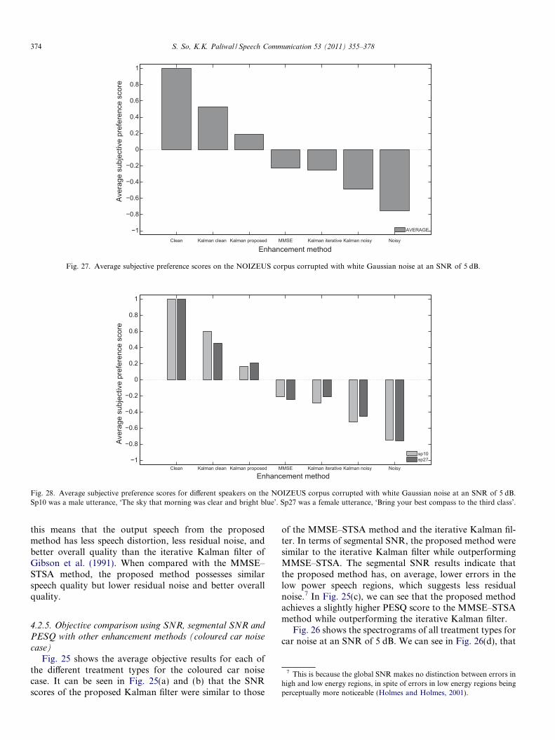
Fig. 28. Average subjective preference scores for different speakers on the NOIZEUS corpus corrupted with white Gaussian noise at an SNR of 5 dB.Sp10 was a male utterance, ‘The sky that morning was clear and bright blue’. Sp27 was a female utterance, ‘Bring your best compass to the third class’.


this means that the output speech from the proposedmethod has less speech distortion, less residual noise, andbetter overall quality than the iterative Kalman filter ofGibson et al. (1991). When compared with the MMSE–STSA method, the proposed method possesses similarspeech quality but lower residual noise and better overallquality.

7 This is because the global SNR makes no distinction between errors inhigh and low energy regions, in spite of errors in low energy regions beingperceptually more noticeable (Holmes and Holmes, 2001).


PESQ with other enhancement methods (coloured car noise

case)

Fig. 25 shows the average objective results for each ofthe different treatment types for the coloured car noisecase. It can be seen in Fig. 25(a) and (b) that the SNRscores of the proposed Kalman filter were similar to those

of the MMSE–STSA method and the iterative Kalman fil-ter. In terms of segmental SNR, the proposed method weresimilar to the iterative Kalman filter while outperformingMMSE–STSA. The segmental SNR results indicate thatthe proposed method has, on average, lower errors in thelow power speech regions, which suggests less residualnoise.7 In Fig. 25(c), we can see that the proposed methodachieves a slightly higher PESQ score to the MMSE–STSAmethod while outperforming the iterative Kalman filter.

Fig. 26 shows the spectrograms of all treatment types forcar noise at an SNR of 5 dB. We can see in Fig. 26(d), that


the iterative Kalman filter has reduced a lot of the noise inthe background but suffers from random residual peaks,which result in popping noises, as noticed in informal lis-tening tests. The MMSE–STSA method (Fig. 26(e)) canbe seen to introduce a spread of residual background noise.In contrast, the proposed Kalman filter in Fig. 26(g) can beseen to produce little-to-no observable residual noise.

Therefore, the Dolph–Chebychev analysis window withlarge side lobe attenuation and long 80 ms frame lengthshave improved the objective enhancement performance ofthe Kalman filter for coloured car noise.

4.2.6. Objective comparison using composite measures with

other enhancement methods (coloured car noise case)

Table 5 shows the average composite measures (SIG,BAK, OVRL) for the proposed Kalman filter comparedwith the other enhancement methods at 5 dB SNR of carnoise. We can see that the proposed Kalman filter achievesthe highest scores for all three composite measures in theKalman ‘family’ of methods, apart from the ideal case(Kalman clean). However, when compared with theMMSE–STSA method, the proposed method producesspeech with more speech distortion but similar residualnoise suppression. The cause of speech distortion can bepinpointed to over-suppression of the Kalman gain trajec-tory in the speech regions, which increases the contributionof the predicted component.

4.2.7. Subjective comparison using blind AB listening tests

Fig. 27 shows the average preference scores from thesubjective listening tests. We can see that the proposed Kal-man filter was preferred on average over all other methodsexcept for the Kalman filter with clean-speech-derivedLPCs and clean speech. The significance of this result canbe appreciated when we consider that the proposed methodinvolved the use of longer frames and a special taperedanalysis window only. Fig. 28 shows the average preferencescores for each of the two utterances. The listeners also pre-ferred on average the proposed Kalman filter for bothutterances over the other methods except for the Kalmanclean method and clean speech.

5. Conclusion

In this paper, we have analysed the effect of poor linearpredictive coefficient estimates on the performance of theKalman filter for speech enhancement. Higher-than-usualprediction errors due to the presence of noise result in largeKalman gain values, even during regions where speechenergy is low. Since the Kalman gain regulates the contri-bution of the noisy observation to the output, large Kal-man gain values result in more residual noise beingpassed through to the output, which can be annoying tothe listener, as errors in low speech energy regions are moreperceptible. By using tapered windows (such as the Dolph–Chebychev window) during LPC estimation, the influenceof additive noise on the Kalman gain was suppressed,

which resulted in lower residual noise. We have also shownthat overlapped frames are beneficial to the Kalman filterwhen long frames and tapered analysis windowing areused. The proposed Kalman filter, which uses two itera-tions for LPC estimation, Dolph–Chebychev windowingin the first iteration, and long and overlapped 80 msframes, was found to have improved on conventionalKalman filtering schemes and in objective and subjectivelistening tests.

Acknowledgments

The authors would like to acknowledge and thank theanonymous reviewers for their expert opinions during thereview process. Their valuable insights as well as carefulguidance have greatly enhanced the clarity and breadthof this paper.

Appendix A. The relative importance of accurate LPC and

excitation variance estimates in Kalman filtering

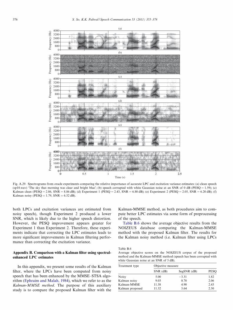
In this appendix, we investigate the relative importanceof accurate LPCs and excitation variance estimates in theKalman filter by performing two oracle Kalman filteringexperiments on a speech file (sp10.wav) that has been cor-rupted with white Gaussian noise at an SNR of 0 dB:

� Experiment 1: with clean LPCs + noisy excitationvariances.� Experiment 2: with noisy LPCs + clean excitation

variances.

The aim is to gain some insight into whether theenhancement performance of the Kalman filter can beimproved by correcting either the excitation variance orLPC estimates, as we have shown earlier in this paper thattapered windows reduce the bias of the excitation varianceof the autocorrelation method. It should be stressed thoughthat the excitation variance and LPCs are dependent toeach other, so the application of tapered windows willinfluence both parameters.

The spectrograms as well as the PESQ scores and SNRsare shown in Fig. A.29. We can see in the spectrogramsthat when noisy excitation variances are used with cleanLPC estimates in Fig. A.29(d) (Experiment 1), theenhanced speech contains some coloured residual noise,which is consistent with our analysis of the dependenceof the Kalman gain on the excitation variance of the model.On the other hand, in Fig. A.29(e) (Experiment 2), wherenoisy LPCs are paired with clean excitation variance esti-mates, we can see that the residual noise is much lowerbut the speech appears to be distorted (and is more notice-able in the low frequency range). Also, the remaining resid-ual noise appears to exist only in the speech regions.

While observing the objective results, we can see that theenhanced speech from both Experiments 1 and 2 have ahigher PESQ score than the noisy Kalman filter (where

0800

1600240032004000

Freq

uenc

y (H

z)

(a)

0800

1600240032004000

Freq

uenc

y (H

z)(b)

0800

1600240032004000

Freq

uenc

y (H

z)

(c)

0800

1600240032004000

Freq

uenc

y (H

z)

(d)

0800

1600240032004000

Freq

uenc

y (H

z)

(e)

Time (s)0 2.5

0

4000

Freq

uenc

y (H

z)

0 0.5 1 1.5 2 2.50

8001600240032004000

(f)

Fig. A.29. Spectrograms from oracle experiments comparing the relative importance of accurate LPC and excitation variance estimates: (a) clean speech(sp10.wav) ‘The sky that morning was clear and bright blue’; (b) speech corrupted with white Gaussian noise at an SNR of 0 dB (PESQ = 1.59); (c)Kalman clean (PESQ = 2.86, SNR = 8.86 dB); (d) Experiment 1 (PESQ = 2.43, SNR = 6.80 dB); (e) Experiment 2 (PESQ = 2.05, SNR = 6.20 dB); (f)Kalman noisy (PESQ = 1.79, SNR = 6.52 dB).


both LPCs and excitation variances are estimated fromnoisy speech), though Experiment 2 produced a lowerSNR, which is likely due to the higher speech distortion.However, the PESQ improvement appears greater forExperiment 1 than Experiment 2. Therefore, these experi-ments indicate that correcting the LPC estimates leads tomore significant improvements in Kalman filtering perfor-mance than correcting the excitation variance.

Table B.6Average objective scores on the NOIZEUS corpus of the proposedmethod and the Kalman-MMSE method (speech has been corrupted withwhite Gaussian noise at an SNR of 5 dB).

Treatment type Objective measure

SNR (dB) SegSNR (dB) PESQ

Noisy 5.00 �3.31 1.82Kalman noisy 9.03 0.70 2.06Kalman-MMSE 11.58 4.90 2.43Kalman proposed 11.32 5.64 2.50

Appendix B. Comparison with a Kalman filter using spectral-

enhanced LPC estimates

In this appendix, we present some results of the Kalmanfilter, where the LPCs have been computed from noisyspeech that has been enhanced by the MMSE–STSA algo-rithm (Ephraim and Malah, 1984), which we refer to as theKalman-MMSE method. The purpose of this auxiliarystudy is to compare the proposed Kalman filter with the

Kalman-MMSE method, as both procedures aim to com-pute better LPC estimates via some form of preprocessingof the speech.

Table B.6 shows the average objective results from theNOIZEUS database comparing the Kalman-MMSEmethod with the proposed Kalman filter. The results forthe Kalman noisy method (i.e. Kalman filter using LPCs

0

800

1600

2400

3200

4000

Freq

uenc

y (H

z)

(a)

Time (s)0 2.5

0

4000

Freq

uenc

y (H

z)

0 0.5 1 1.5 2 2.50

800

1600

2400

3200

4000(b)

0

800

1600

2400

3200

4000(c)

0 0.5 1 1.5 2 2.5Time (s)

0

800

1600

2400

3200

4000(d)

Fig. B.30. Spectrograms comparing the Kalman-MMSE method with the proposed Kalman filter: (a) clean speech (sp10.wav) ‘The sky that morning wasclear and bright blue’; (b) speech corrupted with white Gaussian noise at an SNR of 5 dB (PESQ = 1.59); (c) Kalman-MMSE (PESQ = 2.41); (d) Kalmanproposed (PESQ = 2.52).


from unprocessed noisy speech) are also provided. We cansee that both the Kalman-MMSE and the proposed Kal-man filter have achieved improvements over Kalman noisy,which may be attributed to more accurate LPC estimates.It is interesting to note that the proposed Kalman filter(which applied the Dolph–Chebychev window duringLPC analysis and used long and overlapping frames) hasproduced enhanced speech with a higher segmental SNRand PESQ score than the Kalman-MMSE (which usesthe more sophisticated MMSE–STSA algorithm). Theseobjective results are consistent with the spectrograms inFig. B.30, where the enhanced speech from the proposedKalman filter can be seen to contain less residual noise thanthe enhanced speech from the Kalman-MMSE method.Informal listening of the speech files confirmed that theproposed Kalman filter produced less residual noise thanthe Kalman-MMSE method, though the latter methodproduced less speech distortion.

References

Astrom, K.J., Wittenmark, B., 1997. Computer-Controlled Systems:Theory and Design, third ed.. In: Prentice Hall Information andSystem Sciences Series Prentice-Hall, New Jersey.

Boll, S., 1979. Suppression of acoustic noise in speech using spectralsubtraction. IEEE Trans. Acoust. Speech, Signal Process. ASSP-27 (2),113–120.

Crochiere, R.E., 1980. A weighted overlap-add method of short-timeFourier analysis/synthesis. IEEE Trans. Acoust. Speech Signal Pro-cess. ASSP-28 (1), 99–102.

Ephraim, Y., Malah, D., 1984. Speech enhancement using a minimum-mean square error short-time spectral amplitude estimator. IEEETrans. Acoust. Speech, Signal Process. 32, 1109–1121.

Ephraim, Y., Van Trees, H.L., 1995. A signal subspace approach forspeech enhancement. IEEE Trans. Speech Audio Process. 3, 251–266.

Erkelens, J.S., Broersen, P.M.T., 1997. Bias propagation in the autocor-relation method of linear prediction. IEEE Trans. Speech AudioProcess. 5 (2), 116–119.

Gabrea, M., Grivel, E., Najim, M., 1999. A single microphone Kalmanfilter-based noise canceller. IEEE Signal Process. Lett. 6 (3), 55–57.

Gannot, S., Burshtein, D., Weinstein, E., 1998. Iterative and sequentialKalman filter-based speech enhancement algorithms. IEEE Trans.Speech Audio Process. 6 (4), 373–385.

Gibson, J.D., Koo, B., Gray, S.D., 1991. Filtering of colored noise forspeech enhancement and coding. IEEE Trans. Signal Process. 39 (8),1732–1742.

Hayes, M.H., 1996. Statistical Digital Signal Processing and Modeling.John Wiley, New Jersey.

Haykin, S., 2002. Adaptive Filter Theory, fourth ed.. In: Prentice HallInformation and System Sciences Series Prentice-Hall, New Jersey.

Holmes, J.N., Holmes, W.J., 2001. Speech Synthesis and Recognition,second ed. CRC Press.

Hu, Y., Loizou, P., 2006a. Evaluation of objective measures for speechenhancement. In: Proc. INTERSPEECH 2006, pp. 1447–1450.

Hu, Y., Loizou, P., 2006b. Subjective comparison of speech enhancementalgorithms. In: Proc. IEEE Int. Conf. Acoust. Speech, SignalProcessing, Vol. 1. pp. 153–156.

Kalman, R.E., 1960. A new approach to linear filtering and predictionproblems. J. Basic Eng. Trans. ASME 82, 35–45.

Kay, S.M., 1993. Fundamentals of Statistical Signal Processing. In:Prentice Hall Signal Processing Series, Vol. 1. Prentice-Hall, NewJersey.

Li, C.J., 2006. Non-Gaussian, non-stationary, and nonlinear signalprocessing methods – with applications to speech processing andchannel estimation. Ph.D. Thesis, Aarlborg University, Denmark.

Lim, J.S., Oppenheim, A.V., 1978. All-pole modeling of degraded speech.IEEE Trans. Acoust. Speech Signal Process. ASSP-26, 197–210.

Ma, N., Bouchard, M., Goubran, R.A., 2006. Speech enhancement usinga masking threshold constrained Kalman filter and its heuristicimplementations. IEEE Trans. Speech Audio Process. 14 (1), 19–32.

Makhoul, J., 1975. Linear prediction: a tutorial review. Proc. IEEE 63 (4),561–580.

Mehra, M.K., 1970. On the identification of variances and adaptiveKalman filtering. IEEE Trans. Autom. Control AC-15 (2), 175–184.

Ohya, T., Suda, H., Miki, T., 1994. 5.6 kbits/s PSI-CELP of the half-ratePDC speech coding standard. In: IEEE 44th Vehicular TechnologyConf., pp. 1680–1684.

Paliwal, K.K., Basu, A., 1987. A speech enhancement method based onKalman filtering. In: Proc. IEEE Int. Conf. Acoust. Speech, SignalProcessing, Vol. 12. pp. 177–180.

Rix, A., Beerends, J., Hollier, M., Hekstra, A., 2001. Perceptualevaluation of speech quality (PESQ), an objective method forend-to-end speech quality assessment of narrowband telephonenetworks and speech codecs. ITU-T Recommendation P.862. Tech.rep., ITU-T.


So, S., Paliwal, K.K., Sep. 2008. A long state vector Kalman filterfor speech enhancement. In: Proc. Int. Conf. Spoken LanguageProcessing. pp. 391–394.

Sorqvist, P., Handel, P., Ottersten, B., 1997. Kalman filtering for lowdistortion speech enhancement in mobile communication. In: Proc.IEEE Int. Conf. Acoust. Speech, Signal Processing, Vol. 2. pp. 1219–1222.

Wang, T., Koishida, K., Cuperman, V., Gersho, A., Collura, J.S., 2002. A1200/2400 bps coding suite based on MELP. In: IEEE Workshop onSpeech Coding.

Wiener, N., 1949. The Extrapolation, Interpolation, and Smoothing ofStationary Time Series with Engineering Applications. Wiley, NewYork.

Date post:	15-May-2018
Category:	Documents
Upload:	tranthuy
View:	215 times
Download:	0 times

Suppressing the influence of additive noise on the Kalman ... · for low residual noise speech...

Documents