There is a very large variety of techniques for 3D andrange estimation. Therefore, we will mention onlysome of them. One common approach includes pro-jection of a grating and computing the gradients ob-tained in the image [1–5]. The main disadvantage ofthis type of estimation is that the gradients are ob-tained only in locations with height changes that areusually very space limited and shadowed. Since theheight estimation in this approach is cumulative, amiss of a certain gradient (height change) accumu-lates an error. In addition the technique will obtainthe height change only in the direction perpendicularto the projected grating. If the height change coin-cides with the grating direction no gradient will beobtained.Other 3D techniques involve projection of a line on
the object and scanning the object with that line. The
height might be obtained based on the curvature ofthe projected line [6–11]. The main problem withthose approaches is in the fact that the object mustbe static during the scanning process, otherwise theheight estimation is blurred. Such approaches willnot work for motion estimation.
Another technique is high speed scanning based onactive laser triangulation and a variety of fast to evenreal-time scanners [12]. A completely different ap-proach is based upon stereometric structured lighttechnique where active projection of patterns isviewed from various angles by the camera [13,14].The accuracy of all previously mentioned techniquesdepends on the angle between the object and the pro-jector and the camera or, as in triangulation [15–17],on the angle that the object creates with the twocameras.
Some other approaches are based upon diffractiveoptical elements that project a pattern that variesalong the axial direction of light’s propagation andthat way the type of pattern seen by the camera pro-vides the designation of the distance [18]. However,
in this type of approach the axial resolution of rangeestimation as well as the transversal resolution arevery limited.Holography allows the extraction of the phase of
the object, although the recording is done in intensity[19–23]. In analog holography the recording of an in-tensity pattern that is a result of interference is doneon a photo film, while a reference beam is projectedside by side with the light reflected from the object.The reconstruction is done by illuminating the filmwith the same reference beam. In digital holography[24] the interference pattern generated from the ob-ject and the reference wave is recorded onto an imagesensor, and reconstruction is done with a computerby numerical propagation methods (e.g., convolution[25,26], angular spectrum [27], and Fresnel–Kirchh-off [28,29]). The worse resolution of digital imagingmedia as compared with analog holographic medialimits the maximum angle between interferingbeams to a few degrees.The use of an in-line setup permits the measure-
ment of the object complex amplitude distributionby using phase shifting interferometry [30,31]. Simi-larly, Iemmi et al. [32] applied a point diffraction in-terferometer to digital holography using phaseshifting steps controlled by means of a liquid crystaldevice (LCD). That way they could obtain both am-plitude and phase distributions and visualizationof a 3D object by simple propagation of the calculateddistributions using computer tools. One of the mostuseful applications of digital holography is micro-scopy. Digital in-line microscopy with numerical re-construction [33,34] provides a powerful techniquefor lensless imaging when a low-density object is im-aged. Note however that digital holographic micro-scopy is also done in off-axis geometry, for exampleas presented in [35–38].Another interesting approach for 3D is based upon
using the coherence of a light source. If the coherencelength is short, only surface variations that are smal-ler than this length will generate interference fringes[39,40]. By shifting the sample each time, the fringeswill appear in different transversal locations and the3D topography of the sample can be mapped. For ex-ample, in optical coherence tomography [41,42], thecoherence length of the light source is used in orderto interfere only with light reflected from a very cer-tain layer inside the biomedical sample. A similarconcept is used in digital holography, where 3D topo-graphy of the sample can be mapped without trans-versal scanning [43,44]. In addition, various paperswere also published about tomography in digital ho-lography where rotation of the specimen or modifica-tion of the illuminated wave was used to extract theprofile [45–47].In this paper we present two approaches that are
related to digital holography in order to estimate the3D profile of reflective as well as transmissive ob-jects. The first approach is based upon illuminatinga reflective object with light source of given coher-ence length. The coherence length may be relatively
long. However, the contrast of the fringes within thislength will vary. We map our source by measuringthe contrast of the interference fringes versus axialposition. This will now be our lookup table for the3D estimation. Now, after placing our reflective ob-ject into the system we capture a single image (wedo not shift the object and scan as in [48]) and com-pute the locale contrasts of the fringes. By comparingthis contrast with the lookup table we extract the 3Dinformation. This approach extracts the 3D informa-tion from a single image, and its accuracy does notdepend on the triangulation angle.
The second approach deals with a technique allow-ing extraction of profile of transmissive objects espe-cially in microscopy and mainly with biomedical andcell research, where in many cases the sample istransparent (phase-only objects). The approach re-sembles the concept of tomography [49]. We use di-gital holography in order to extract the phaseprofile obtained from an object while we slightly varythe angle of the specimen. The profile of the sample isextracted from at least two angles despite the factthat the profile variations generate phase changesof more than 2π. Actually the usage of at least twoangles is required in order to solve the phase wrap-ping ambiguity existing in all the other approachessuch as phase shifting [30].
If the sample is uniform in its profile and there isvariation only in the refraction index, this approachcan be used as well in order to estimate the refractionindex of the transparent sample (various approachesexist for determination of the refractive index indigital holography such as in [38,50–53]). By usingmore than two angles, the precision for the profile es-timation (or for the refraction index) is increased. Ap-plying the proposed approach in microscopy forresearch of cells offers several advantages such asimaging of phase-only objects without the need totranslate the phase information into an amplitudeinformation, extraction of the true profile withoutphase wrapping ambiguities, and possibility for esti-mating the refraction index.
In Section 2 we present the theory and explain theoperation principle of each one of the two approaches.In Section 3 we present some preliminary experi-mental results. The paper is concluded in Section 4.
2. Operation principle
A. Partial coherence for 3D
The first approach that is presented in this paperdeals with extraction of 3D information based uponthe partial coherence of the light source. Assumingtwo interfering beams, the resulting field distribu-tion equals
where Ai, φi are the amplitude and the phase of eachbeam, respectively; λ is the wavelength; and θ is thedifference between their angles of arrival to the de-tection plane. The intensity in this case equals
ItotðxÞ ¼ hEtotðx; tÞE�totðx; tÞi
¼ A21 þ A2
2 þ 2A1A2hcosðϕ1ðtÞ − ϕ2ðtÞÞi
· cos�4π sin θ
λ x
�; ð2Þ
where < … > designates time averaging operation.For two coherent sources: hcosðϕ1ðtÞ − ϕ2ðtÞÞi ¼cosðϕ1 − ϕ2Þ, and for incoherent sources hcosðϕ1ðtÞ−ϕ2ðtÞÞi ¼ 0. Therefore it is clear that the amount ofcoherence determines the contrast of the generatedinterference fringes.Given a certain laser, its coherence length inver-
sely depends on its spectral bandwidth (its colors’content). What we propose in this technique is an ap-proach for mapping the 3D information of reflectiveobjects. We assume that only a single interferenceimage is captured. Since we are talking about reflec-tive objects (and not diffusive) no imaging lens isneeded for the setup in order to relate the contrastof the interference fringes and the resulting 3D pro-file with the spatial coordinates of the object.Basically we use Michelson’s interferometer con-
figuration, where there is a mirror in the referencepath and an object in the second optical path. Sinceλ=ð2 sin θÞ is the spatial period of the fringes we willuse a relatively large angle difference θ (of, say, a fewdegrees, e.g., 1°) such that the interference fringesare obtained with high spatial frequency and there-fore high spatial lateral resolution for the 3D map-ping (for instance with an angle of 1° we may havespatial lateral resolution of 15 μm for a wavelengthof 500nm),We start by calibrating our system and instead of
an object we place a mirror (therefore the setup is aMichelson interferometer with two mirrors both inthe reference plane and in the object path). We scanwith the mirror and map the change of the local spa-tial contrast of the interference fringes versus theaxial position of the reference mirror. This result willbe used as our lookup table for later on to translatethe contrast of the image to real 3D information ofthe reflective object. The smaller the axial rangewe wish to map, the shorter should be the coherencelength of our light source.After computing the lookup table, we place the ob-
ject back into the interferometer setup (we take outthe mirror that before was temporally placed in itsposition) and capture a single image. We computethe local contrast of the fringes for every transversalposition in the captured image. By comparing the re-sult with our lookup table the profile of the objectmay be estimated. Note that by tuning the spectralwidth of our light source we vary its coherencelength, and therefore we can control or adjust the ax-ial range that is usable for the 3D mapping.
The proposed approach is good for extracting the3D information or the profile of reflective objects,while its main application can be in the field of mi-croscopy or in the microelectronic industry (inspec-tion of various wafers) since the shorter thecoherence length, the better the axial resolution.The main advantage of this approach in comparisonwith other approaches is that it does not use trian-gulation, and therefore its precision is not dependenton the angle between the object and the two cameras[15–17] or the camera and the projection module [6].Another advantage is that the 3D information is ex-tracted from a single image, while no axial scanningis required [48], and therefore this method may beused for real time mapping of live specimens.
Note that since lasers usually have several spec-tral lines (due to their Fabry–Perot interferometer),the coherence length is a periodic function, while itsperiod inversely depends on the total spectral widthof the source (the spectral separation between thelines multiplied by the number of lines) and the over-all number of periods inversely depends on the widthof each spectral line (actually it will be the ratio be-tween the total spectral width and the width of eachspectral line). In our experiments for the demonstra-tion of this approach we used Nd:YAG laser with ax-ial periodicity for the coherence function of close to2mm (overall spectral width of about 150GHz).The coherence length should be application depen-dent. For instance, for application of chip inspection(in microelectronics) or for microscopy, the coherencelength should be in the range of about 0:1mm Forapplication of pattern recognition, computer vision,and gaming, the range should be a few tens of cmor even more.
An important comment is related to the relationbetween the lateral field of view and the axial reso-lution obtained by this approach. Across the field ofview the fringes do not have uniform contrast sincerays coming to the external regions of the field ofview travel longer optical paths in comparison withthe rays coming to the center of the field. The differ-ence of the contrast along the field of view can bemapped as part of the calibration process in whichthe lookup table is prepared. However, the field ofview must be limited such that for a given coherencelength and thus for a given axial resolution thefringes at the borders of the field of view will stillhave detectable contrast. Mathematically, given asensor having b sampling bits, i.e., 2b gray levelsof dynamic range, and angle of θ between the two in-terfering optical paths, and a sensor with a lateraldimension of L, the best possible axial resolutionδz that may be obtained will be
δz ≈ L × sin θ2b
; ð3Þ
which means that the contrast of the fringes at theedges of the image should not be below the minimallevel of quantization.
Another important note is related to the number ofsampling pixels. In every period of the interferencefringes one needs more than 2 sampling pixels (atleast twice as much as required by Nyquist’s sam-pling theorem) in order to estimate the contrast.The double number of pixels is needed to have suffi-ciently accurate estimation. Therefore if the anglebetween the two interfering paths is 1° and thusthe period of the fringes is 15 μm for a wavelengthof 500nm, then the size of the pixels should not belarger than about 4 μm in order to have sufficientsamples for the contrast estimation. Thus, since4 μm is about the smallest available pixel size, thevalue of about 15 μm is the maximal lateral resolu-tion for the 3D mapping.Since the 3D mapping in this approach is based
upon local contrast estimation, the reflectivity ofthe objects can affect this estimation, and it mustbe addressed in the calibration stage as well as inthe profile estimation procedure. In the next section,in Eqs. (7) and (8) we demonstrate that in propercomputing procedure this effect is not too significant.We show that even in the extreme case of a siliconwafer having reflectivity of only 30% for intensityand a mirror in the reference path having reflectivityof 100%, the effect over the contrast estimation isonly 15%. Therefore, if the inspected object comprisesseveral materials, each having a different refractionindex and therefore different reflectivity, the maxi-mal error will be smaller than 15% [e.g., see experi-mental results of Fig. 5(a)]. In the real case thevariation in the reflectivity will not be 70% (100%in comparison with 30%) but rather smaller thanthat, which will affect the estimation by only a fewpercent. By proper normalization the generated er-ror may be reduced (e.g., by estimating the contrastin plurality of neighbor sampling points and aver-aging the results).The proposed technique does not include an ima-
ging lens, and therefore the lateral resolution forthe 3D mapping is affected not only by the coherenceof the source or the capability to estimate local con-trast but also by the diffraction, which blurs spatialfeatures especially near steep borders. The blurringspot or the spatial resolution δxz that is forced by thediffraction after free space propagation of a distanceof Z can be estimated by the following relation:
where δx is the standard deviation of the smallestspatial feature in the original object (we assume aGaussian distribution), λ is the optical wavelength,and Z is the free space propagation distance. In ordernot to lose resolution one needs
Z ≤2π · δx2
λ ; ð5Þ
assuming again spatial resolution of δx ¼ 15 μm andwavelength of 500nm, the length of the free space
path should not be larger than approximatelyZ ¼ 3mm. Basically, even such short propagationdistances may be feasible in real configurations (withsmall beam splitters that can be integrated on top ofthe detection array). However, in the proposed setupthe dimensions of the beam splitter prevent us ofgoing to Z being below 1 cm. Therefore, the spatialresolution will be reduced to δx ¼ 30 μm.
B. Phase unwrapped profiling
Phase-shifting and holography-based approaches areused for extraction of 3D information. The main pro-blem of those approaches is the phase wrapping, i.e.,the mapping range should not be larger than one wa-velength otherwise there is an ambiguity [30]. There-fore such approaches are not suitable for profileestimation having a large range of topographic var-iations. Here we suggest using a tomography-basedapproach in order to solve the phase wrapping am-biguity.
The idea is to project a transmissive object whoseprofile we wish to extract, from several angles. Then,by digital holography to recover the phase of everyexposure. The phase recovery by digital holographyincludes performing a Fourier transform over thefringe pattern and then taking out the informationaround the first diffraction order, putting it aroundthe center of the axes, and performing the inverseFourier transform. The obtained result is back freespace propagated (using the Fresnel transform) afree space distance that exists between the specimenand the recording array. The phase after the backfree space propagation is extracted, and it is the re-sult for the desired phase that is related to the profileof the inspected object.
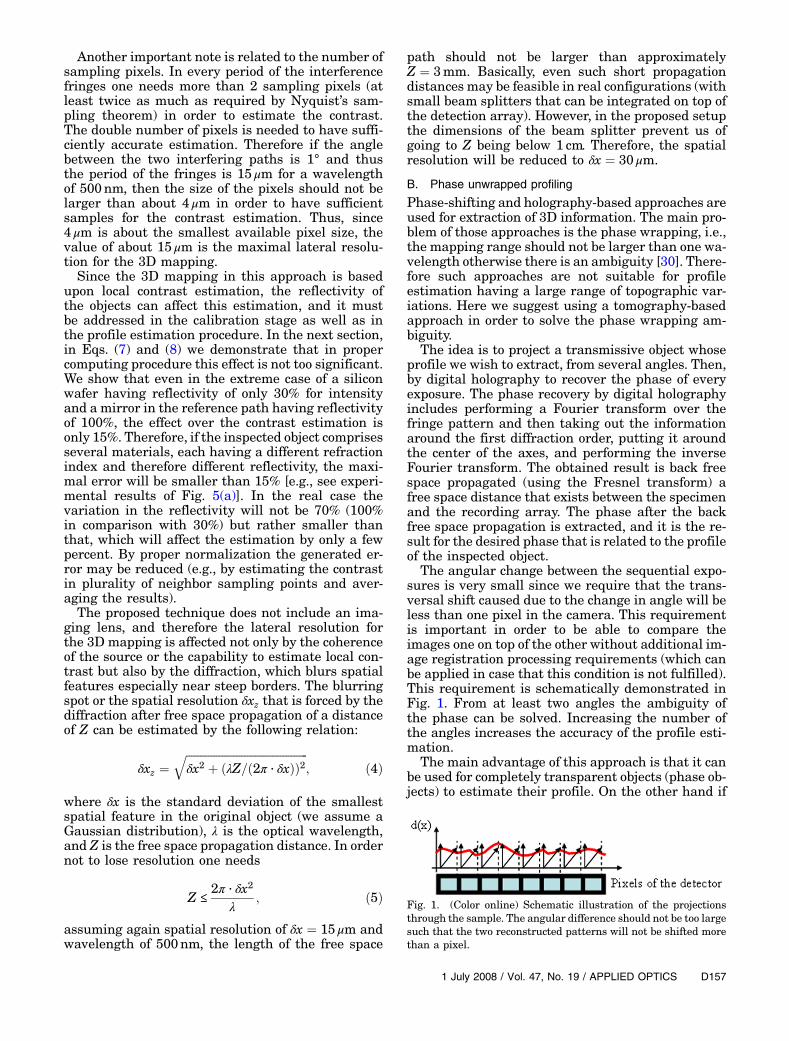
The angular change between the sequential expo-sures is very small since we require that the trans-versal shift caused due to the change in angle will beless than one pixel in the camera. This requirementis important in order to be able to compare theimages one on top of the other without additional im-age registration processing requirements (which canbe applied in case that this condition is not fulfilled).This requirement is schematically demonstrated inFig. 1. From at least two angles the ambiguity ofthe phase can be solved. Increasing the number ofthe angles increases the accuracy of the profile esti-mation.
The main advantage of this approach is that it canbe used for completely transparent objects (phase ob-jects) to estimate their profile. On the other hand if
Fig. 1. (Color online) Schematic illustration of the projectionsthrough the sample. The angular difference should not be too largesuch that the two reconstructed patterns will not be shifted morethan a pixel.
the profile is known, this technique can be used inorder to estimate the refraction index of the phasespecimen [45–47]. The main application is in micro-scopy for biomedical applications where this proce-dure can assist in imaging the phase-only sampleswithout the need to translate the phase informationinto amplitude information. This approach may alsobe used in the microelectronics industry especiallyfor wafer inspection.The optical configuration is basically a Mach–
Zehnder interferometer where the sample is placedon a rotating stage and its angle of position can beaccurately tuned. Assuming that a sample is illumi-nated at two different angles θ1 and θ2, then twophase readouts can be extracted (one per each image)after proper processing (as done in digital hologra-phy). We denote by aðxÞ and bðxÞ the phase extractedin the first and the second projection, respectively:
�2πndðxÞλ cos θ1
�modf2πg ¼ a ðxÞ;
�2πndðxÞλ cos θ2
�modf2πg ¼ bðxÞ; ð6Þ
where λ is the wavelength, n is the refraction index ofthe sample, and dðxÞ is the true (unwrapped) profilethat we wish to extract. mod is the mathematical op-eration of modulo.Plotting the theoretical a and b values for width d
varying from 0:5 μm up to 20 μm in steps of 10nmyields the result presented in Fig. 2. One maysee that indeed the mapping is one to one and com-paring the measured a and b values with the existinglookup table can lead to the estimation of d.It is clear that increasing the number of angles re-
duces the estimation error. Assuming that one usesM angles, then the number of possible combinationsof a pair of angles will be equal to MðM − 1Þ, and
therefore since each one of those combinations willproduce an uncorrelated estimation for the profiled, the overall error will be reduced by a factorof
An experimental setup that is based upon Michelsoninterferometer was constructed in the lab (see inFig. 3 both the schematic sketch of the setup andits real image). As opposed to the setup in [48], noimaging lens is needed since we deal with reflectiverather than diffusive objects. First, we have con-structed the lookup table by placing a mirror insteadof the object and axially shifting (i.e., scanning with)the mirror of the reference beam while measuringthe contrast for all of its axial positions. We used
Fig. 2. (Color online) One to one mapping between variousheights of the profile dðxÞ and the readout phases aðxÞ and bðxÞ.
Fig. 3. (Color online) Experimental setup for the partial coherence experiment. B.S, beam splitter.
an Nd:YAG laser at a wavelength of 512nm. The con-trast chart versus the axial shift appears in Figs. 4(a)and 4(b). Actually we did this measurement twice fortwo different alignments of the setup. Obviously thecontrast and the lookup table depend on the specificalignment of the optical setup.In the next step we placed a reflective object
containing several silicon wafers (taken from themicroelectronics industry). We performed two experi-ments; in the first the two wafers were positionedside by side on top of a mirror. In the second experi-ment we used three wafers, two placed on top of thethird one.As previously mentioned a very interesting prop-
erty of the proposed configuration is that it almostdoes not depend on the exact reflectivity of the sur-face of the object that we map. What we mean is thatthe spatial contrast variations mainly depend on thetopography rather than the reflectivity profile of theobject. This is a very important property since other-wise the method would not have been that applic-
able. Let us now mathematically estimate thesensitivity to the reflectivity of the inspected object.The contrast C is defined as
C ¼ Imax − Imin
Imax þ Imin¼ 2jr1r2j
jr1j2 þ jr2j2; ð7Þ
where Imax and Imin are the maximal and the mini-mal intensities, respectively, of the interferencefringe. r1 and r2 are the fields’ reflectivity for thetwo optical paths of the interferometer. This is ofcourse in the case of perfect alignment and ideal con-ditions. In our experiments we used silicon wafers,while the lookup table was obtained with mirrors.The reflectivity of silicon can be computed usingFresnel coefficients. At normal angles
jrj ¼����n1 − n2
n1 þ n2
����: ð8Þ
In the case of silicon surrounded by air we have ap-proximately n1 ¼ 3:5 and n2 ¼ 1, and thereforejrj ¼ 0:556. In the case of the mirror, the reflectivitycoefficient jrj is close to 1. If we place those numbersin Eq. (7) we see that instead of having maximal con-trast of 1 we will have a contrast of 0.85. Therefore, inthe extreme case of a perfect mirror and a silicon wa-fer which is far from being a mirror, the variation dueto the change in the object’s reflectivity is only by15%. Obviously in the practical case this differenceis much smaller since the mirror's reflectivity isnot exactly 1 and the alignment is not perfect. Alsowhen we know the type of substrate (e.g., silicon) wecan perform a normalization of contrasts according tothe ratio from Eq. (7).
Note that in the visible range the silicon will havenot only a real but also an imaginary part (attenua-tion) for the refractive index. However, the imaginarypart of the refractive index is about 200 times smal-ler than the real part and therefore was neglected inour computation.
Following this line we performed two experimentswith silicon wafers. The thickness of each wafer was765 μm with standard variation for the thickness of10 μm. In both experiments the objects were placed inthe setup (each in turn) and the interference patternwas captured. The local contrast of the fringes wascomputed, and it was compared with the results fromthe lookup table of Figs. 4(a) and 4(b). Since the or-ientation or the tilting angles of the fringes are un-known and they are varied along the captured image,the estimation of the local contrast in an automaticmanner was not trivial. Our solution for this problemwas to use the Radon transform for the computationof the local contrasts (the Radon transform producesa high value if the direction of its projections is par-allel to the direction of the interference fringes).Therefore the Radon transform assisted us in auto-matic allocation of the tilting direction of the fringessuch that correct computing of contrast was feasible.An example of fringes and their corresponding Radon
Fig. 4. (Color online) Experimental mapping of the contrast chartversus the axial shift of one of the mirrors. (a) and (b) are for twodifferent alignments. (c) Fringes and their corresponding Radontransform.
transform (to be used for the estimation of the con-trast) is presented in Fig. 4(c). At the angles corre-sponding to the tilting of the fringes, at the Radontransform one will get a periodic pattern with highvalues of gray levels. At that angle the contrastshould be computed, and this is the tilting angle ofthe fringes. After computing an image of local con-trasts, a topography image for the specimen can beextracted.The experimental results, including the image of
the object and the interference pattern of the fringesas well as the numerical extraction of the local con-trasts, appear in Fig. 5. The image in Fig. 5(a) corre-sponds to the alignment, and the lookup table ofFig. 4(a), and the image of Fig. 5(b) corresponds tothe alignment of 4(b). After the measurements ofthe local contrast we saw in both cases that indeed:
• In Fig. 5(a) the difference in thickness betweenthe two small silicon wafers and the mirror is around765 μm (as anticipated), while the difference betweenthe two wafers (upper left and upper right) is ap-proximately of the order of magnitude of 20–30 μm.This is obtained by comparing the reference chart
of Fig. 4(a) with the measurements of the contrastin Fig. 5(a). The relevant values were marked onthe chart in Fig. 4(a).
• In Fig. 5(b) the difference in thickness betweenthe wafer on the left side and the two wafers on theright side is approximately 765 μm (as anticipated),while the difference in the thickness of the two wa-fers on the right side (right/up and right/ down) isabout 10–15 μm. This is obtained by comparing thereference chart of Fig. 4(b) with the measurementsof the contrast in Fig. 5(b). The relevant values weremarked on the chart in Fig. 4(b).
Note that since the lookup charts ofFigs. 4(a) and 4(b) are periodic, there are severalpositions that have had the contrast values (ofFig. 5(a) and 5(b)) measured, each resulting in a dif-ferent possible result for the height estimation. Ingeneral, in the proposed approach we do not intendto go beyond half a period of the reference lookupcharts, i.e., beyond half the period of the axial coher-ence length, and that way we intend to avoid inter-pretation ambiguity. It is even recommended to havethe working zone much smaller than that in order tostay in the linear region of the lookup (i.e., calibra-tion) chart in order to have a linear relation betweenthe changes in contrast and their correspondingheight/topography interpretation. The object thatwe tested in our preliminary experiment did not haveperfect fit to the coherence length of our laser, andtherefore some ambiguity in interpretation was gen-erated. By looking in the a priori known range wecould estimate the precise value of the profile. Ob-viously in a real application proper fitting shouldbe made between the coherence length of the sourceand the range of profiles that we aim to inspect in ourspecimen. In addition, generally speaking the lookuptables have a discrete set of values. Therefore, if themeasured contrast falls in between two values of thetable an interpolation procedure is applied in orderto have the precise profile estimation. Also note thatthe experimental setup of Fig. 3 is used only for re-flective objects such as those that we took from thesilicon industry. The 3D information was extractedfrom a single image, and therefore it is useful for realtime inspection applications.
B. Phase unwrapped profiling
The experiment included construction of Mach–Zehnder-based interferometer, while the sample tobe inspected was placed on top of a high precision ro-tation stage. The image of the setup appears alongwith its schematic sketch in Fig. 6. We used a He–Nelaser with a long coherence length (more than a fewtens of cm). The inspected object was a small rectan-gle generated in photolithography process on top of aglass substrate. The refraction index of the glass sub-strate was 1.5, while that of the photoresist was 1.6(after developing). The photoresist used was SU-8.For comparison, the profile of the rectangle wasmapped using an Alpha-Step profile meter and ap-
Fig. 5. (Color online) Image of the object used for the partial co-herence experiment and the obtained interference pattern withthe extracted local contrasts. (a) Two silicon wafers positionedon a mirror. (b). Two silicon wafers positioned on top of a third si-licon wafer.
pears in Fig. 7, where each pixel was 0:8 μm. There-fore the dimensions of the rectangle were about0:7mm by 2:4mm. The profile height was approxi-mately 10 μm (see Fig. 7 for a mesh chart).Next we tried to verify the experimental data of
Fig. 7 by applying our tomography-based approach.We used projection at two angles separated by 1degree. The obtained results are seen in Fig. 8. InFig. 8(a) one may see the two phase images obtainedfor the two projection angles. The phase images wereobtained using digital holography. The algorithmwas as follows: we performed a Fourier transformover the recorded fringe pattern, and then we tookout the information around the first diffraction order.We placed it around the center of the axes and per-formed an inverse Fourier transform. The obtainedresult was back free space propagated, using theFresnel transform by the free space distance existingbetween the specimen and the recording array. Thephase of the obtained distribution after the back freespace propagation was extracted. In Fig. 8(b) we com-puted the profile of the sample. Each pixel in the fig-
ure is a pixel of the camera that is 6:7 μm by 6:7 μm.The thickness appearing in the figure is in meters.
Onemay see that the results obtained using digitalholography with multiple projections correspondwell to the experimental measurements of Fig. 7 bothin the transversal dimensions of the phase segment(about 0:7mm by 2:4mm) and by its thickness (about10 μm). Therefore, the proposed approach may be im-plemented in microscopy in extraction of profiles oftransmissive phase objects (objects as biologicalcells).
4. Conclusions
In this paper we have demonstrated two approachesfor extraction of the profiles and the 3D informationof objects. In the first case we used an approach thatis based upon the coherence property of the lightsource that affected the local contrast of the obtainedinterference fringes. From a single image we werecapable of estimating the 3D information of a reflec-tive object, and no scanning in time was required.The main advantage of this approach is that it fitswell for real time object inspection, its accuracy doesnot depend on triangulation angle, and its axial pre-cision can be tuned just by varying the spectral band-width of the light source and by changing itscoherence length. In the second approach we havedemonstrated a technique that has some similarityto tomography and that uses digital holography inorder to extract the phase of transmissive objectsfrom the plurality of slightly varied angles. Propercomputation allows true estimation of the profilewhile solving the problem of the phase ambiguitydue to phase wrapping every 2π. This approach al-lows imaging of phase-only transmissive objects,and in cases when the profile of the objects is knownit allows estimating its refraction index.
This work was supported by FEDER funds and theSpanish Ministerio de Educacion y Ciencia under theProject FIS2007-60626.
Fig. 7. (Color online) Experimental reconstruction using an Al-pha-Step profile meter. Each pixel is 0:8 μm.
Fig. 6. (Color online) Experimental setup for the profile extraction concept based upon multiple angle projection.
References1. Y. G. Leclerc and A. F. Bobick, “The direct computation of
height from shading,” in IEEE Conference on ComputerVision & Pattern Recognition (IEEE, 1991), pp. 552–558.
2. R. Zhang and M. Shah, “Shape from intensity gradient,” IEEETrans. Syst. Man Cybern., Part A Syst. Humans 29, 318(1999).
3. “Height recovery from intensity gradients,” in IEEE Confer-ence on Computer Vision & Pattern Recognition (IEEE, 1994),pp. 508–513 .
4. B. K. P. Horn, “Height and gradient from shading,” Int. J. Com-put. Vis. 5, 37–76 (1990).
5. A. M. Bruckstein, “On shape from shading,” Comput. Vis.Graph. Image Process. 44, 139–154 (1988).
6. M. Asada, H. Ichikawa, and S. Tjuji, “Determining of surfaceproperties by projecting a stripe pattern,” in Proceedings ofthe International Pattern Recognition Conference (IEEE,1986), pp.1162–1164.
7. M. Asada, H. Ichikawa, and S. Tsuji, “Determining surface or-ientation by projecting a stripe pattern,” IEEE Trans. PatternAnal. Mach. Intell. 10, 749–754 (1988).
8. S. Winkelbach and F. M. Wahl, “Shape from single stripe pat-tern illumination,” in (DAGM 2002) Pattern Recognition, Vol.2449 of Lecture Notes in Computer Science, L. Van Gool, ed.(Springer, 2002), pp. 240–247.
9. T. P. Koninckx and L. Van Gool, “Efficient, active 3D acquisi-tion, based on a pattern-specific snake,” in (DAGM 2002) Pat-tern Recognition, Vol. 2449 of Lecture Notes in ComputerScience, L. Van Gool, ed. (Springer, 2002), pp. 557–565.
10. R. Kimmel, N. Kiryati, and A. M. Bruckstein, “Analyzingand synthesizing images by evolving curves with theOsher-Sethian method,” Int. J. Comput. Vis. 24, 37–56(1997).
11. G. Zigelman, R. Kimmel, and N. Kiryati, “Texure mappingusing surface flattening via multi-dimensional scaling,” IEEETrans. Vis. Comput. Graph. 8, 198–207 (2002).
12. L. Zhang, B. Curless, and S. M. Seitz, “Rapid shape acquisitionusing color structured light and multi pass dynamic program-ming,” presented at the 1st International Symposium on 3DData Processing Visualization and Transmission (3DPVT),Padova, Italy, July, 2002.
13. P. Besl, “Active optical range imaging sensors,” Mach. VisionApplications 1, 127–152 (1988).
14. E. Horn and N. Kiryati, “Toward optimal structured light pat-terns,” presented at the International Conference on RecentAdvances in 3-D Digital Imaging and Modeling, Ottawa,Canada, May 1997.
Fig. 8. (Color online) Experimental reconstruction. (a) Phase reconstruction for two projection angles that were separated by 1 degree.(b) Profile reconstruction. Each pixel is the pixel of the camera that was 6:7 μm. The alleviation thickness is in meters.
16. G. Hausler and D. Ritter, “Parallel three-dimensional sensingby color-coded triangulation,” Appl. Opt. 32, 7164–7170(1993).
17. R. G. Dorsch, G. Hausler, and J. M. Herrmann, “Laser trian-gulation: fundamental uncertainty in distancemeasurement,”Appl. Opt. 33, 1306–1312 (1994).
18. D. Sazbon, Z. Zalevsky, and E. Rivlin, “Qualitative real-timerange extraction for preplanned scene partitioning using laserbeam coding,” Pattern Recogn. Lett. 26, 1772–1781 (2005).
19. D. Gabor, “Microscopy by reconstructed wave fronts,” Proc. R.Soc. London, Ser. A 197, 454–487 (1949).
20. E. N. Leith, “Overview of the development of holography” J.Imaging Sci. Technol. 41, 201–204 (1997).
21. E. N. Leith and J. Upatnieks, “Wavefront reconstructionand communication theory,” J. Opt. Soc. Am. 52, 1123–1130(1962).
22. Y. N. Denisyuk, “On the reproduction of the optical propertiesof an object by the wave fields of its scattered radiation,” Opt.Spectrosc. 15, 279–284 (1964).
23. R. V. Pole, “3-D imaging and holograms of objects illuminatedin white light,” Appl. Phys. Lett. 10, 20–22 (1967).
24. A. Stern and B. Javidi, “Improved-resolution digital hologra-phy using the generalized sampling theorem for locally band-limited fields,” J. Opt. Soc. Am. A 23, 1227–1235 (2006).
25. U. Schnars and W. P. O. Juptner, “Digital recording andnumerical reconstruction of holograms,” Meas. Sci. Technol.13, R85–R101 (2002).
26. T. Colomb, F. Montfort, J. Kühn, N. Aspert, E. Cuche, A.Marian, F. Charrière, S. Bourquin, P. Marquet, and C.Depeursinge, “Numerical parametric lens for shifting, magni-fication, and complete aberration compensation in digitalholographic microscopy,” J. Opt. Soc. Am. A 23, 3177–3190(2006).
27. C. Mann, L. Yu, C. -M. Lo, andM. Kim, “High-resolution quan-titative phase-contrast microscopy by digital holography,”Opt. Express 13, 8693–8698 (2005).
28. E. Cuche, F. Bevilacqua, and C. Depeursinge, “Digital hologra-phy for quantitative phase-contrast imaging,” Opt. Lett. 24,291–293 (1999).
29. P. Ferraro, S. De Nicola, A. Finizio, G. Coppola, S. Grilli, C.Magro, and G. Pierattini, “Compensation of the inherent wavefront curvature in digital holographic coherent microscopy forquantitative phase-contrast imaging,” Appl. Opt. 42, 1938–1946 (2003).
30. I. Yamaguchi and T. Zhang, “Phase shifting digital hologra-phy,” Opt. Lett. 22, 1268–1270 (1997).
31. J. H. Bruning, D. R. Herriot, J. E. Gallagher, D. P. Rosenfeld, A.D. White, and D. J. Brangaccio, “Digital wavefront measuringinterferometer for testing optical surfaces and lenses,” Appl.Opt. 13, 2693–2703 (1974).
32. C. Iemmi, A. Moreno, and J. Campos, “Digital holography witha point diffraction interferometer,” Opt. Express 13, 1885–1891 (2005).
33. W. Xu, M. H. Jericho, I. A. Meinertzhagen, and H. J. Kreuzer,“Digital in-line holography of microspheres,” Appl. Opt. 41,5367–5375 (2002).
34. J. Garcia-Sucerquia, W. Xu, S. K. Jericho, P. Klages, M. H.Jericho, and H. J. Kreuzer, “Digital in-line holographic micro-scopy,” Appl. Opt. 45, 836–850 (2006).
35. E. Cuche, P. Marquet, and C. Depeursinge, “Simultaneous am-plitude-contrast and quantitative phase-contrast microscopyby numerical reconstruction of Fresnel off-axis holograms,”Appl. Opt. 38, 6994–7001 (1999).
36. P. Marquet, B. Rappaz, P. J. Magistretti, E. Cuche, Y. Emery, T.Colomb, and C. Depeursinge, “Digital holographic microscopy:
a noninvasive contrast imaging technique allowing quantita-tive visualization of living cells with subwavelength axialaccuracy,” Opt. Lett. 30, 468–470 (2005).
37. B. Kemper and G. von Bally, “Digital holographic microscopyfor live cell applications and technical inspection,” Appl. Opt.47, A52–A61 (2008).
38. B. Rappaz, P. Marquet, E. Cuche, Y. Emery, C. Depeursinge,and P. Magistretti, “Measurement of the integral refractive in-dex and dynamic cell morphometry of living cells with digitalholographic microscopy,” Opt. Express 13, 9361–9373 (2005).
39. V. Mico, J. García, C. Ferreira, D. Sylman, and Z. Zalevsky,“Spatial information transmission using axial temporal coher-ence coding,” Opt. Lett. 32, 736–738 (2007).
40. J. Rosen and A. Yariv, “General theorem of spatial coherence:application to three-dimensional imaging,” J. Opt. Soc. Am. A13, 2091–2095 (1996).
41. D. Huang, E. A. Swanson, C. P. Lin, J. S. Schuman, W. G. Stin-son, W. Chang, M. R. Hee, T. Flotte, K. Gregory, C. A. Puliafito,and J. G. Fujimoto, “Optical coherence tomography,” Science254, 1178 (1991).
42. J. M. Schmitt, “Optical coherence tomography (OCT): a re-view,” IEEE J. Sel. Top. Quantum Electron. 5, 1205 (1999).
43. P. Massatsch, F. Charrière, E. Cuche, P. Marquet, and C. D.Depeursinge, “Time-domain optical coherence tomographywith digital holographic microscopy,” Appl. Opt. 44, 1806–1812 (2005).
44. G. Pedrini and S. Schedin, “Short coherence digital hologra-phy for 3D microscopy,” Optik (Jena) 112, 427–432 (2001).
45. F. Charrière, A. Marian, F. Montfort, J. Kuehn, T. Colomb, E.Cuche, P. Marquet, and C. Depeursinge, “Cell refractive indextomography by digital holographic microscopy,” Opt. Lett. 31,178–180 (2006).
46. F. Charrière, N. Pavillon, T. Colomb, C. Depeursinge, T. J.Heger, E. A. D. Mitchell, P. Marquet, and B. Rappaz, “Livingspecimen tomography by digital holographic microscopy: mor-phometry of testate amoeba,” Opt. Express 14, 7005–7013(2006).
47. W. Choi, C. Fang-Yen, K. Badizadegan, R. R. Dasari, and M. S.Feld, “Extended depth of focus in tomographic phase micro-scopy using a propagation algorithm,” Opt. Lett. 33, 171–173(2008).
48. T. Dresel, G. Hausler, and H. Venzke, “Three-dimensional sen-sing of rough surfaces by coherence radar,”Appl. Opt. 31, 919–925 (1992).
49. H. Stark and H. Peng, “Shape estimation in computer tomo-graphy from minimal data,” J. Opt. Soc. Am. A 5, 331–337(1988).
50. T. Yasokawa, I. Ishimaru, M. Kondo, S. Kuriyama, T. Masaki,K. Takegawa, and N. Tanaka, “A method for measuring thethree-dimensional refractive index distortion of single cellusing proximal two-beam optical tweezers and a phase shift-ing Mach-Zehnder interferometer,” Opt. Rev. 14, 161–164(2007).
51. B. Kemper, S. Kosmeier, P. Langehanenberg, G. Von Bally, I.Bredebusch, W. Domschke, and J. Schnekenburger, “Integralrefractive index determoination of living suspension cells bymultifocus digital holographic phase contrast microscopy,” JBiomed. Opt. 12, 054009 (2007).
52. N. Lue, G. Popescu, T. Ikeda, R. R. Dasari, K. Badizadegan,and M. S. Feld, “Live cell refractometry using microfluidic de-vices,” Opt. Lett. 31, 2759–2761 (2006).
53. M. M. Hossain, D. S. Mehta, and C. Shakher, “Refractive indexdetermination: an application of lensless Fourier digital holo-graphy,” Opt. Eng. 45, 106203–106207 (2006).