SYMBOLIC COMPUTATION OF CONSERVATION …whereman/papers/Poole-PhD-Thesis-2009.pdfNONLINEAR PARTIAL...

SYMBOLIC COMPUTATION OF CONSERVATION LAWS OF

NONLINEAR PARTIAL DIFFERENTIAL EQUATIONS

USING HOMOTOPY OPERATORS

by

Loren Douglas Poole

A thesis submitted to the Faculty and the Board of Trustees of the Colorado

School of Mines in partial fulfillment of the requirements for the degree Doctor of Phi-

losophy (Mathematical and Computer Sciences)

Golden, Colorado

Date

Signed:Loren Douglas Poole

Signed:Dr. Willy Hereman

Thesis Advisor

Golden, Colorado

Date

Signed:Dr. Dinesh P. Mehta

Professor and HeadDepartment of Mathematical and Computer Sciences

ii

ABSTRACT

A mathematical method is developed for the purpose of constructing conserva-

tions laws for nonlinear partial differential equations (PDEs) in multiple space dimen-

sions. The method is developed in the language of calculus, the calculus of variations

and linear algebra, so that it is accessible to researchers in different fields. The method is

algorithmic and has been implemented in the syntax of Mathematica, a major and com-

monly used computer algebra system. The software package, ConservationLawsMD.m,

symbolically computes conservation laws for polynomial PDEs that can be written as

nonlinear evolution equations.

With ConservationLawsMD.m, conservation laws are computed for many PDEs

from mathematical physics, fluid dynamics, and soliton theory. Test cases are formed us-

ing conservation laws for the Zakharov-Kuznetsov equation, the Kadomtsev-Petviashvili

equation and other well-known PDEs. Previously unknown conservation laws are given

for several PDEs, including the Manakov-Santini system and the two-dimensional Gard-

ner equation.

A second software package, HomotopyIntegrator.m, consists of code for the ho-

motopy operator in ConservationLawsMD.m. The homotopy operator integrates one-

dimensional exact expressions involving unspecified functions, or inverts a divergence

on two- or three-dimensional exact expressions. The one-dimensional homotopy code is

designed to supplement Mathematica’s Integrate function. Since Mathematica does

not have a function to invert divergences, the two- and three-dimensional homotopy

codes provide a new and versatile tool for vector calculus.

When computing conservation laws, verification of their independence is of key

importance. A third software package, IndependenceTest.m implements a comprehen-

sive method for testing if densities are independent. Although this code is also part of

ConservationLawsMD.m, the package IndependenceTest.m can be used as a stand-alone

tool for researchers working on conservation laws.

iii

iv

TABLE OF CONTENTS

ABSTRACT . . . . . . . . . . . . . . . . . . . . . . . . . . . . . . . . . . . . . . iii

LIST OF FIGURES . . . . . . . . . . . . . . . . . . . . . . . . . . . . . . . . . . ix

LIST OF TABLES . . . . . . . . . . . . . . . . . . . . . . . . . . . . . . . . . . . xi

ACKNOWLEDGEMENTS . . . . . . . . . . . . . . . . . . . . . . . . . . . . . . xii

CHAPTER 1 INTRODUCTION . . . . . . . . . . . . . . . . . . . . . . . . . . 1

1.1 Previous Work . . . . . . . . . . . . . . . . . . . . . . . . . . . . . . . . 3

1.2 New Contributions . . . . . . . . . . . . . . . . . . . . . . . . . . . . . . 5

CHAPTER 2 NOTATION AND DEFINITIONS . . . . . . . . . . . . . . . . . . 11

CHAPTER 3 EXAMPLES OF CONSERVATION LAWS OF NONLINEAR PDES

IN (2+1)- AND (3+1)-DIMENSIONS . . . . . . . . . . . . . . . . 19

3.1 The Zakharov-Kuznetsov Equation . . . . . . . . . . . . . . . . . . . . . 21

3.2 The (3+1)-Dimensional Equation for Non-stationary Transonic Gas Flow 24

3.3 The (2+1)-Dimensional Gardner Equation . . . . . . . . . . . . . . . . . 28

CHAPTER 4 TOOLS FOR THE COMPUTATION OF CONSERVATION LAWS:

THE ZEROTH-EULER OPERATOR . . . . . . . . . . . . . . . . 31

4.1 General Definitions . . . . . . . . . . . . . . . . . . . . . . . . . . . . . . 31

4.2 The Euler-Lagrange Equations . . . . . . . . . . . . . . . . . . . . . . . . 33

4.3 A Proof for the Exactness Theorem . . . . . . . . . . . . . . . . . . . . . 38

CHAPTER 5 INDEPENDENCE OF CONSERVED DENSITIES . . . . . . . . 43

5.1 Terms that are Divergences or Divergence-Equivalent . . . . . . . . . . . 44

5.2 Trivial Conservation Laws . . . . . . . . . . . . . . . . . . . . . . . . . . 47

5.3 Equivalent Densities . . . . . . . . . . . . . . . . . . . . . . . . . . . . . 48

5.4 Linear Combinations . . . . . . . . . . . . . . . . . . . . . . . . . . . . . 49

v

CHAPTER 6 TOOLS FOR THE COMPUTATION OF CONSERVATION LAWS:

THE HOMOTOPY OPERATOR . . . . . . . . . . . . . . . . . . 55

6.1 The Original Homotopy Operator . . . . . . . . . . . . . . . . . . . . . . 57

6.2 Where is the Homotopy in the Homotopy Operator? . . . . . . . . . . . . 59

6.3 Reformulation of the Homotopy Operator Integrand . . . . . . . . . . . . 60

6.3.1 The Homotopy Operator for One Independent Variable . . . . . . 61

6.3.2 The Homotopy Operator for Two Independent Variables . . . . . 70

6.3.3 The Homotopy Operator for Three Independent Variables . . . . 76

6.4 Removing Divergence-Free Terms . . . . . . . . . . . . . . . . . . . . . . 77

6.5 Limitations of the Homotopy Operator . . . . . . . . . . . . . . . . . . . 80

CHAPTER 7 CONSTRUCTION OF CONSERVATION LAWS FOR NONLIN-

EAR PDES . . . . . . . . . . . . . . . . . . . . . . . . . . . . . . . 83

7.1 Conservation Laws for the Zakharov-Kuznetsov Equation . . . . . . . . . 83

7.1.1 Establishing a Scaling Symmetry . . . . . . . . . . . . . . . . . . 84

7.1.2 Construction of a Candidate Density . . . . . . . . . . . . . . . . 87

7.1.3 Determination of the Actual Density . . . . . . . . . . . . . . . . 90

7.1.4 Calculation of the Flux . . . . . . . . . . . . . . . . . . . . . . . . 93

7.2 Conservation Laws for the Non-stationary Transonic Gas Flow Equation 94

7.2.1 Scaling Symmetry for the NTGF Equation . . . . . . . . . . . . . 95

7.2.2 Construction of Candidate Densities . . . . . . . . . . . . . . . . 96

7.2.3 Determination of the Actual Densities . . . . . . . . . . . . . . . 98

7.2.4 Calculation of the Flux and Inversion of the Transformation . . . 100

7.3 Conservation Laws for the Gardner Equation . . . . . . . . . . . . . . . . 101

7.3.1 Establishing a Scaling Symmetry . . . . . . . . . . . . . . . . . . 101

7.3.2 Determination of the Density . . . . . . . . . . . . . . . . . . . . 102

7.3.3 Calculation of the Flux and Inversion of the Transformation . . . 104

CHAPTER 8 CONSERVATION LAWS FOR PDES IN MULTI-DIMENSIONS 107

8.1 Kadomtsev-Petviashvili Equations . . . . . . . . . . . . . . . . . . . . . . 108

8.1.1 The Kadomtsev-Petviashvili Equation . . . . . . . . . . . . . . . 108

8.1.2 The Potential Kadomtsev-Petviashvili Equation . . . . . . . . . . 111

vi

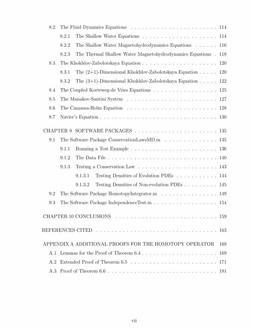
8.2 The Fluid Dynamics Equations . . . . . . . . . . . . . . . . . . . . . . . 114

8.2.1 The Shallow Water Equations . . . . . . . . . . . . . . . . . . . . 114

8.2.2 The Shallow Water Magnetohydrodynamics Equations . . . . . . 116

8.2.3 The Thermal Shallow Water Magnetohydrodynamics Equations . 118

8.3 The Khokhlov-Zabolotskaya Equation . . . . . . . . . . . . . . . . . . . . 120

8.3.1 The (2+1)-Dimensional Khokhlov-Zabolotskaya Equation . . . . . 120

8.3.2 The (3+1)-Dimensional Khokhlov-Zabolotskaya Equation . . . . . 122

8.4 The Coupled Korteweg-de Vries Equations . . . . . . . . . . . . . . . . . 125

8.5 The Manakov-Santini System . . . . . . . . . . . . . . . . . . . . . . . . 127

8.6 The Camassa-Holm Equation . . . . . . . . . . . . . . . . . . . . . . . . 128

8.7 Navier’s Equation . . . . . . . . . . . . . . . . . . . . . . . . . . . . . . . 130

CHAPTER 9 SOFTWARE PACKAGES . . . . . . . . . . . . . . . . . . . . . . 135

9.1 The Software Package ConservationLawsMD.m . . . . . . . . . . . . . . 135

9.1.1 Running a Test Example . . . . . . . . . . . . . . . . . . . . . . . 136

9.1.2 The Data File . . . . . . . . . . . . . . . . . . . . . . . . . . . . . 140

9.1.3 Testing a Conservation Law . . . . . . . . . . . . . . . . . . . . . 143

9.1.3.1 Testing Densities of Evolution PDEs . . . . . . . . . . . 144

9.1.3.2 Testing Densities of Non-evolution PDEs . . . . . . . . . 145

9.2 The Software Package HomotopyIntegrator.m . . . . . . . . . . . . . . . 149

9.3 The Software Package IndependenceTest.m . . . . . . . . . . . . . . . . . 154

CHAPTER 10 CONCLUSIONS . . . . . . . . . . . . . . . . . . . . . . . . . . . 159

REFERENCES CITED . . . . . . . . . . . . . . . . . . . . . . . . . . . . . . . . 163

APPENDIX A ADDITIONAL PROOFS FOR THE HOMOTOPY OPERATOR 169

A.1 Lemmas for the Proof of Theorem 6.4 . . . . . . . . . . . . . . . . . . . . 169

A.2 Extended Proof of Theorem 6.5 . . . . . . . . . . . . . . . . . . . . . . . 171

A.3 Proof of Theorem 6.6 . . . . . . . . . . . . . . . . . . . . . . . . . . . . . 181

vii

viii

LIST OF FIGURES

9.1 The menu that appears when ConservationLawsMD[] is initiated. . . 136

9.2 Page 1 of the menu listing the first ten multi-dimensional PDEs. . . . . . 137

9.3 A list of weights for the (2+1)-dimensional Zakharov-Kuznetsov equation. 138

9.4 Information provided by ConservationLawsMD.m when the program ter-

minates. A conservation law for the (2+1)-dimensional Zakharov-Kuznetsov

equation is shown. . . . . . . . . . . . . . . . . . . . . . . . . . . . . . . 139

9.5 The contents of the data file, d zk2d.m, for the (2+1)-dimensional Zakharov-

Kuznetsov equation. . . . . . . . . . . . . . . . . . . . . . . . . . . . . . 141

9.6 The result for testing the density of (9.3) for the Riemann System (9.1). . 146

9.7 The result from ConservationLawsMD.m verifying the density for the

Kadomtsev-Petvishvili evolution equations (8.2). . . . . . . . . . . . . . . 148

9.8 A sample data file of densities for the potential Kadomtsev-Petviashvili

equation. Note that three densities in this file are independent and one

is not. . . . . . . . . . . . . . . . . . . . . . . . . . . . . . . . . . . . . . 155

9.9 The evaluation of a density for the potential Kadomtsev-Petviashvili equa-

tion based on previously established independent densities. . . . . . . . . 157

ix

x

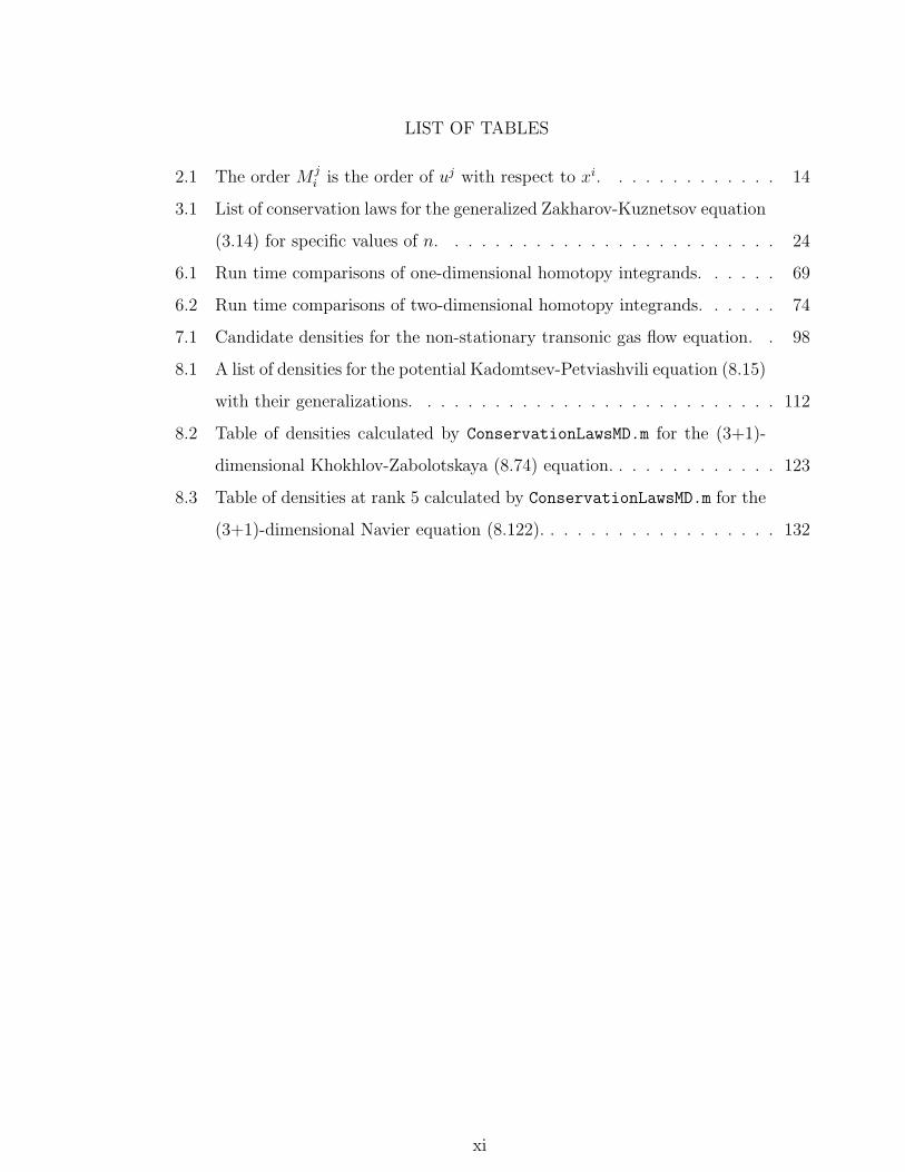
LIST OF TABLES

2.1 The order M ji is the order of uj with respect to xi. . . . . . . . . . . . . 14

3.1 List of conservation laws for the generalized Zakharov-Kuznetsov equation

(3.14) for specific values of n. . . . . . . . . . . . . . . . . . . . . . . . . 24

6.1 Run time comparisons of one-dimensional homotopy integrands. . . . . . 69

6.2 Run time comparisons of two-dimensional homotopy integrands. . . . . . 74

7.1 Candidate densities for the non-stationary transonic gas flow equation. . 98

8.1 A list of densities for the potential Kadomtsev-Petviashvili equation (8.15)

with their generalizations. . . . . . . . . . . . . . . . . . . . . . . . . . . 112

8.2 Table of densities calculated by ConservationLawsMD.m for the (3+1)-

dimensional Khokhlov-Zabolotskaya (8.74) equation. . . . . . . . . . . . . 123

8.3 Table of densities at rank 5 calculated by ConservationLawsMD.m for the

(3+1)-dimensional Navier equation (8.122). . . . . . . . . . . . . . . . . . 132

xi

ACKNOWLEDGEMENTS

Many thanks to my advisor, Dr. Willy Hereman, for the numerous hours he has

spent guiding me through this project. With his insight and considerable knowledge,

he was constantly able to suggest improvements and get me through tough spots. His

“what if” questions often led to new discoveries and better methods, and he kept me on

my toes by being constantly able to pick the one example that would create difficulties

for my programs.

I also wish to thank the Department of Mathematical and Computer Science at

CSM for their support and for allowing me to teach classes. The opportunity to work

in the classroom has provided valuable experience for my academic career.

An undergraduate student, John-Bosco Tran, was most helpful by running and

testing the conservation laws program and checking to see that the conservation laws

presented in this dissertation were typeset correctly.

Thanks also goes to the National Science Foundation for their support. My

research was supported in part under grant no. CCF-083783.

As well, I would like to thank Dr. Thomas Wolf for allowing me access to his

CONLAW programs, as well as Dr. Jan Sanders and Dr. Bhimsen Shivamoggi for re-

sponding with confirmation of results from my programs.

xii

For Charles and Nina

xiii

xiv

CHAPTER 1

INTRODUCTION

To a person familiar with physics, conservation of mass, momentum, energy,

electric charge, and other quantities are well known. A conserved quantity moves or

flows from one place to another; portions of it do not magically appear or disappear. A

conservation law is a mathematical equation that describes how the quantity is affected

by flow. In a dynamics problem, the amount of material flowing out of a closed region,

or the flux of the material, is equal to the change of the density times the change in

volume of the material contained in the closed region. Irrespective of their physical

meaning, the dynamics terms “conserved density” and its associated “flux” will be used

to represent the two dependent pieces of a conservation law.

Many partial differential equations (PDEs) or systems thereof that model physical

situations exhibit conservation laws such as the conservation of mass, momentum, or

energy. However, special nonlinear PDEs may also have a multitude of conservation

laws without a physical meaning. Conservation laws are related to the symmetries of a

PDE, a connection shown in a remarkable theorem proved by Emmy Noether in 1918

[54]. Noether proved that every conservation law for an invariant Euler-Lagrange system

corresponds to a Lie symmetry for that system. That is, if a variational principle can be

determined for a symmetry of a PDE, a corresponding conservation law can be found.

Her theorem has been used in a wide variety of applications.

A serious study of conservation laws of nonlinear PDEs began in the 1960s with

the investigation of solitary wave and soliton solutions for the Korteweg-de Vries (KdV)

equation. In the 1870s, both Joseph Boussinesq and Lord Rayleigh independently pro-

posed a nonlinear PDE to model the motion of a solitary wave moving in a channel

[28]. In 1895, Diederik Korteweg and Gustav de Vries derived the same equation [46],

which now carries their names. The KdV equation drew little interest until the 1960s.

In 1965, Martin Kruskal and Norman Zabusky were investigating wave motion in a one-

dimensional anharmonic lattice of equal masses [81]. They were trying to solve the FPU

problem, posed by Enrico Fermi, John Pasta, and Stanislaw Ulam, a problem investi-

1

gating how energy is distributed among the many possible oscillations in a nonlinear

lattice [24]. Zabusky and Kruskal found that interacting solitary waves would retain

their shapes after collisions, that is, obey the superposition principle. This occurred de-

spite the fact that the waves were highly nonlinear. Zabusky and Kruskal named these

solitary waves “solitons”, and discovered that in the continuum limit, the KdV equation

modeled the wave behavior and energy distribution they were observing.

At this point, attention turned toward the KdV equation and methods for finding

soliton solutions. Since conservation laws provide information about properties of a PDE,

part of the investigation focused on finding conserved densities for the KdV equation.

The first two conservation laws, representing the conservation of mass and conservation

of energy, had been known for some time. While investigating nonlinear dispersive waves

in 1965, Gerald Whitham discovered the third conservation law [74]. In the same year,

Zabusky and Kruskal computed the fourth and fifth conservation laws, but failed to find

a sixth due to an error in their calculations. The following year, Robert Miura was able

to find a seventh conservation law, then corrected the error in the computations and

found the sixth. Miura went on to discover three more conservation laws, then proved

[52] that an infinite sequence of conservation laws exists for the KdV equation.

The work by Kruskal, Zabusky and Miura, along with John Greene and Clifford

Gardner led to the discovery of a one-parameter family of Backlund transformations

between the solutions of the KdV and modified KdV equations, the discovery of the Lax

pair for the KdV equation, and the Inverse Scattering Transform (IST) for linearizing

the KdV equation [26]. The IST [1] provides a method for finding solitons for a PDE

of all orders. When this can be done, the PDE is said to be completely integrable.

While applying the IST to a PDE can be an onerous task, the existence of an infinite

set of conservation laws indicates that a PDE is completely integrable, and that the

application of the IST is likely to completely solve the PDE. However, the existence

of infinitely many conservation laws is not a prerequisite. Indeed, PDEs that have few

conservation laws have been found to be integrable. The best known example is the

Burgers equation which can be transformed into the heat equation using the Cole-Hopf

transformation [18, 37]. Integrable equations or systems are essential to theoretical

and mathematical physicists, whose goal is to describe and understand the behavior of

2

classical or quantum systems [82].

Why compute conservation laws? First of all, one may wish to know which

physical quantities are conserved in the system described by the PDE. Investigation of

conservation laws can lead to new discoveries in particular, new methods for finding

solutions for PDEs. For example, in the KdV case the investigation of conservation laws

led to the discovery of the IST, a key method to solve nonlinear PDEs. Conservation laws

aid the study of qualitative properties of PDEs, such as bi-Hamiltonian structures and

recursion operators [9]. If constitutive properties have been added to close a system, one

may wish to verify if conserved quantities have remained intact [34]. Conserved densities

also aid in the design of numerical solvers for PDEs [63].

The approach used in this dissertation to compute conservation laws requires tools

from calculus, linear algebra and the calculus of variations. It implements and extends

the method described by Hereman et al. in [35] and by Hereman in [33]. A candidate

density is constructed by forming a linear combination with undetermined coefficients

of differential terms that are invariant under the scaling symmetry of the PDE . The

undetermined coefficients can be calculated by applying the variational derivative to the

time derivative of the candidate density after the density has been rewritten in terms of

the space variables using the PDE. Once the density is known, the flux can be computed

by applying a homotopy operator to invert a divergence. Each phase of this process will

be explained in detail, using examples to clarify the explanations.

1.1 Previous Work

There are many methods for computing conservation laws [35, 53]; all require a

significant amount of computation, which is best done with a computer algebra system

(CAS) such as Mathematica, Maple, or REDUCE. A summary of nine methods for

computing conservation laws is given by Naz [53], of which some have been coded in

CAS. The method used in this dissertation is not mentioned by Naz.

Two previously developed packages written in Mathematica use some of the tech-

niques that will be presented in this dissertation. The package CONDENS.M, written by

Goktas and Hereman [28, 29] calculates conservation laws for (1+1)-dimensional PDEs,

that is, PDEs that have one independent space variable and one independent time vari-

3

able. TransPDEDensityFlux.m, a package written by Adams and Hereman [2, 3], ex-

tends the code in CONDENS.M to work on (1+1)-dimensional PDEs with transcendental

nonlinearities. Neither program will work on a PDE with multiple space dimensions,

and both accept only evolution equations. The methods used in CONDENS.M have also

been extended to compute conservation laws for (1+1)-dimensional differential difference

equations [34].

Two other fully developed programs exist to compute conservation laws, one

by Wolf [76] in REDUCE and one by Cheviakov [15] in Maple. The program GeM by

Cheviakov [15, 16], computes a set of multipliers on the PDE. The multipliers lead to

a determining system of differential equations, based on the symmetries of the PDE,

that yield a conservation law [4, 5]. The method does not require the computation of

a variational principle as required by Noether’s Theorem, but does require that a PDE

be written in Cauchy-Kovalevskaya form, that is, that the PDE be solved in terms of

its highest order derivative(s). Since a conservation law is computed as a divergence, a

homotopy operator is used to invert the divergence [16] to get the density and the flux.

The packages CONLAW1 through CONLAW4 written by Wolf in REDUCE [75, 78]

find conservation laws by solving an over-determined system of differential equations.

All four versions use the program CRACK, a sophisticated solver for systems of differential

equations. CONLAW1 tries to solve the continuity equation directly, while CONLAW3 tries

to find the conservation law and its characteristic [56] concurrently. A characteristic is

an identifying expression that has the same properties as the conservation law. Both

CONLAW2 and CONLAW4 try to find the characteristic function before computing the con-

served density. CONLAW2 uses substitutions based on the PDE, whereas CONLAW4 does not.

While each of these programs can compute conserved densities with explicit dependence

on the independent variables, arbitrary functions, and transcendental nonlinearities, it

may be necessary to use a combination of the programs to find all conservation laws for

a PDE. The complexity of the problem increases very fast as the order for the charac-

teristic function increases, and the systems of differential equations generated become

very large and difficult to solve.

Another method applies Noether’s Theorem to get conservation laws from vari-

ational symmetries [56]. This method is used in the Maple package DE APPLS, a part

4

of the Vessiot suite written by Anderson for computations in the jet space [6]. This

program requires continual input from the user while working with Noether’s theorem

and requires that the symmetries of the PDE have variational principles. The Vessiot

suite is now part of a differential geometry package in Maple, introduced in version 11.

The package was designed by Anderson and Cheb-Terrab [7] and contains the functions

necessary to compute conservation laws. However, all computations are done in the

language of differential forms.

The homotopy operator is used on expressions containing unspecified functions.

The homotopy operator can integrate (by parts) a one-dimensional expression or invert

the divergence of a multi-dimensional expression. The homotopy operator originates in

differential geometry in a proof showing the exactness of the variational complex [56]. It

has since been “translated” from the language of differential geometry into the language

of standard calculus by Hereman et al. [35]. The one-dimensional version given in [35]

was implemented in TransPDEDensityFlux.m [2] to resolve issues with Mathematica”s

Integrate function. The one-dimensional version has also been implemented in Maple

by Deconinck and Nivala [21] and contains a feature for separating an expression into

an integrable part and a nonintegrable part.

1.2 New Contributions

A significant part of the research for this dissertation is the development of

three software packages. All three software packages are written in Mathematica syntax

and do computations symbolically. The leading package, ConservationLawsMD.m, con-

tains all of the algorithms needed to compute conservation laws. Two additional pack-

ages, HomotopyIntegrator.m and IndependenceTest.m are spin offs of Conservation-

LawsMD.m. These are stand-alone packages that can be used in different applications in-

volving conservation laws, and beyond. The algorithms in all three packages follow the

procedures and algorithms for computing conservation laws that will be described in

this dissertation.

In contrast to the programs discussed previously, ConservationLawsMD.m has

several advantages. The program can run on a desktop computer and works on any

system that supports Mathematica. The program does not generate systems of differ-

5

ential equations, nor does it need to compute an Euler-Lagrange system as required by

Noether’s Theorem. The program can be set to run automatically, or the user can inter-

act with the program by providing information he or she may have already computed.

The program runs fast, and reports the conservation laws in notation that is easy to

read. The program also automatically verifies the independence of the densities it com-

putes. In all test cases, the program was able to compute a complete set of conservation

laws, identical to conservation laws given in literature. Several examples of PDEs are

provided in the package for a user to test and explore.

The package ConservationLawsMD.m uses the same general principle based on

the scaling symmetry of the PDE as CONDENS.M, and includes some of the same features.

However, many new algorithms had to be developed to extend the code to (2+1)- and

(3+1)-dimensional PDEs. In general, computing conservation laws in (2+1)- or (3+1)-

dimensions is considerably more complex than computing conservation laws for (1+1)-

dimensional PDEs. As ConservationLawsMD.m was developed, a number of problems

not encountered in CONDENS.M or TransPDEDensityFlux.m had to be overcome. This

led to the design of several features not found in the older programs. These include

• an algorithm that converts a class of non-evolution equations into evolution form.

• a new algorithm for constructing the candidate density, adapted from the idea put

forth in [35].

• a method for constructing candidate densities with explicit independent variables

multiplied to dependent variables.

• a method for testing densities with rational and transcendental terms, as well as

for testing densities with arbitrary functions.

• a method which involves a homotopy operator for finding the flux once the density

is known. In higher dimensions, calculating the flux requires inverting a divergence,

whereas in one dimension the flux can be found using integration by parts. CAS

cannot invert divergences, and in some cases, fail to integrate one-dimensional

expressions involving arbitrary functions that require integration by parts.

• a method for removing “curl” terms from a vector that is an inverted divergence.

6

• an algorithm for checking for trivial conservation laws or conservations laws that

are either equivalent to one another, or a combination of lower order conservation

laws.

The set of (1+1)-dimensional examples of PDEs in CONDENS.M consists almost

entirely of evolution equations. Very few (2+1)- and (3+1)-dimensional PDEs are evo-

lution equations, so an algorithm was developed to “transform” equations into evolution

equations. The algorithm used for generating a candidate density in CONDENS.M does not

produce the most desirable candidate when more than one independent space variable is

involved. A new method, which uses the variational derivative and linear algebra, works

efficiently and produces the most desirable candidate density by removing unnecessary

terms.

The package ConservationLawsMD.m can only compute polynomial conservation

laws. A polynomial conservation law is polynomial in the dependent variables, however,

terms may be multiplied by polynomial functions of independent variables. Most (1+1)-

dimensional PDEs have polynomial conservation laws where terms are not multiplied by

independent variables. The (1+1)-dimensional version, CONDENS.M, does not attempt to

compute terms multiplied by independent variables. The procedure used in CONDENS.M

produced very few conservation laws for multi-dimensional PDEs. Yet some of these

PDEs were known to be completely integrable, suggesting that an infinite variety of

conservation laws may exist. Conservation laws for higher dimensional PDEs found in

literature exhibited explicit time and space variables in both the density and flux, so the

algorithm for generating a candidate density was modified to generate terms with explicit

time and space variables. Once these modifications were made, ConservationLawsMD.m

was able to consistently reproduce conservation laws in test cases.

Once a candidate density is known, the program CONDENS.M computes the flux us-

ing Mathematica’s Integrate function to do the necessary integration by parts. When

transcendental nonlinearities were added to densities in TransPDEDensityFlux.m, Math-

ematica’s Integrate often failed to do the required integration. In multi-dimensions,

it is necessary to invert a divergence to find the flux. CAS cannot do this. The homotopy

operator solves both of these problems, providing a convenient method for computing

fluxes.

7

The homotopy operator presented in this dissertation has been revised to work

efficiently in code. Two issues arose with the original version that needed to be addressed

before the homotopy operator would become a useful tool. First, the homotopy operator

would produce a “swell” of terms internally, most of which would cancel before producing

a solution. This was especially bad in the three-dimensional case. Using properties of

combinatorics, the homotopy operator has been revised to eliminate the expression swell,

thus generating considerably fewer terms. Secondly, in the multi-dimensional forms,

the vector returned by the homotopy operator after it has inverted a divergence often

contains divergence free or “curl” terms. A method to remove curl terms, based on

linear algebra, has been developed. With these modifications, the homotopy operator

has become a reliable tool for computing fluxes, even on differential expressions with

transcendental or rational terms. However, like any integrator, there are limitations on

what expressions the homotopy operator can integrate.

Since the homotopy operator has been successful on a wide variety of expres-

sions, a second package, HomotopyIntegrator.m, composed of the homotopy operator

code in ConservationLawsMD.m has been created. The package HomotopyIntegrator.m

operates independently of ConservationLawsMD.m and can be used strictly as an inte-

grator. The (1+1)-dimensional code is designed to work in tandem with Mathematica’s

Integrate function. Supposedly, Integrate works on all types of functions, how-

ever, it often has difficulty integrating expressions containing unspecified functions in-

volving transcendental or rational terms. The (2+1)- and (3+1)-dimensional code is an

added feature for Mathematica since there currently is no function or package available

for inverting divergences.

A third package accompanying this dissertation, IndependenceTest.m, also works

independently of ConservationLawsMD.m. The package IndependenceTest.m takes a

list of densities and compares them, checking that each density is independent of the

other densities in the list, then prints a report. It is quite easy to compute two equivalent

densities, but often difficult to recognize that they are equivalent. This package will be

especially useful to researchers using other methods for computing conservation laws,

giving a quick method for verification.

Several multi-dimensional PDEs with applications in fluid dynamics, gas dynam-

8

ics and mechanics are presented with a list of conservation laws for each PDE. Con-

servation laws have been published by various researchers for he Zakharov-Kuznetsov

equation, the non-stationary transonic gas flow equation, the Kadomtsev-Petviashvili

equation, the Khokhlov-Zabolotskaya equation, the shallow water fluid dynamics equa-

tions and the shallow water magnetohydrodynamics equations. These equations are

presented as test cases and their conservation laws are compared to conservation laws

presented in literature. Conservation laws for the Gardner equation, the Manakov-

Santini system, the Camassa-Holm equation and the thermal shallow water magneto-

hydrodynamics equations have not been found in literature to date. The conservation

laws presented for these equations are new. Partial results have been found for Navier’s

equation and the coupled Korteweg-de Vries equation. Some of the conservation laws

for these equations are new.

In Chapter 2, notations are introduced, along with some basic definitions. Chap-

ter 3 contains examples of PDEs along with several of their conservation laws. These

examples will be used in later chapters to demonstrate and emphasize procedures for

calculating conservation laws. Chapters 4 and 6 show the key tools used in the computa-

tion of conservation laws. The zeroth-Euler operator, otherwise known as the variational

derivative from the calculus of variations, is introduced and its role in the Exactness

Theorem is explained in Chapter 4. Chapter 6 shows the development of the homotopy

operator used in the ConservationLawsMD.m and HomotopyIntegrator.m. A discussion

of trivial conservation laws and a method for checking conservation laws for indepen-

dence are given in Chapter 5. Chapter 7 contains a detailed description of how to

compute conservation laws. The PDEs from Chapter 3 will be used to show the pro-

cess and to highlight different techniques required for special situations that arise in the

calculations. Chapter 8 shows additional examples of PDEs with some of their conser-

vation laws, demonstrating the versatility of the program. Chapter 9 gives a description

of the three software packages, ConservationLawsMD.m, HomotopyIntegrator.m, and

IndependenceTest.m and explains how they run. Several examples showing results

from a Mathematica notebook will demonstrate how each algorithm works and highlight

the special features. Finally, Chapter 10 discusses future areas of research, including

suggestions to make the algorithms more universal.

9

10

CHAPTER 2

NOTATION AND DEFINITIONS

Theorems and procedures shown in this dissertation are written in a form that

allows for easy adaptation into the language of Mathematica or other CAS. Indeed, the

procedures that will be described have all been programmed in Mathematica. It will be

left to others to develop similar code in other CAS.

Notation for independent and dependent variables.

Conservation laws are computed for PDEs in (1+1)-, (2+1)-, or (3+1)-dimen-

sions. An (n+1)-dimensional PDE has n independent space variables, x = (x1, . . . , xn)

and a time variable, t. The wording one-, two-, or three-dimensions will be used to

denote the number of independent space variables under consideration, when t acts as

a parameter. The function u = g(x, t) will represent a solution to a nonlinear PDE,

where dependent variable u has N components, that is, u =(u1, u2, . . . , uj, . . . , uN

).

The superscript notation is used in definitions and proofs involving the zeroth-Euler

operator in Chapter 4 and the homotopy operator in Chapter 6. This notation closely

follows the notation used by Olver [56] and has been widely adopted [14, 38, 39, 75]

in this field of research. All concrete examples involving PDEs that occur throughout

this dissertation will have no more than five dependent variables or three independent

space variables. In all examples, x will be taken as x, (x, y), or (x, y, z) for one-, two-

or three-dimensional problems, respectively. Also, for simplicity, the components of u

will be (u, v) instead of (u1, u2). In PDEs where the dependent variables represent given

quantities, appropriate dependent variables will replace components of u. For example,

in the shallow water hydrodynamics equations, (u, v, θ, ψ, h) will be used instead of

(u1, u2, u3, u4, u5).

Notation for partial derivatives.

Partial derivatives on components of u are denoted with a number-variable sub-

script notation. For example, ∂2u∂x2 will be u2x,

∂5u∂x3∂y2

will be u3x2y, and ∂ku∂xk will be ukx.

This notation serves two purposes; it makes multiple partial derivatives easy to repre-

11

sent in operators which involve sums over partial derivatives and it shortens lengthy

differential expressions, making them easier to read.

Notation for jet spaces and differential functions.

The construction of a conservation law requires building a differential expression

based on symmetries of the PDE. The differential expression has terms consisting of

dependent variables and partial derivatives on dependent variables. The coefficients of

these terms are constant or may be functions of the independent variables. Operations

applied to differential expressions will act on the jet space, which is defined as follows.

Definition 2.1. Let X be the space whose coordinate consists of the components of x.

Additionally, let U0 be the space whose coordinate consists of all components of u and

UM be the space whose coordinate consists of all partial derivatives of order M on all

components of u with respect to x. The Cartesian product U0 × U1 × · · · × UM is the

space UM with coordinate u(M) [56]. The M th order jet space, JM [38] is the Cartesian

product X × UM .

A differential function f(x,u(M)(x)) is defined on JM where f is determined by f : X ×

UM −→ R. Differentiations and integrations are carried out with respect to variables in

JM . In all cases where f = f(x,u(M)(x)), while f may contain terms where components

of x are multiplied by components of u and derivatives of components of u, f will not

have terms containing only components of x.

Example 2.1. Let u = (u, v) and x = (x, y), then U0 is the space with coordinate

(u, v), U1 is the space with coordinate (ux, uy, vx, vy), and U2 is the space with coordinate

(u2x, uxy, u2y, v2x, vxy, v2y). The jet space J2 = X×U2 = X×U0×U1×U2 has the coordi-

nate (x,u(2)) = (x, y, u, v, ux, uy, vx, vy, u2x, uxy, u2y, v2x, vxy, v2y). A differential function

f(x,u(2)(x)) is then defined on J2.

Notation for operators acting on differential functions.

Several operators will appear that involve sums over derivatives on the jet space.

The upper limit on the sums will be denoted by M ji , the order of differential function f

for partial derivatives on uj with respect to xi.

12

Example 2.2. Let x = (x1, x2), u = (u1, u2), and f = f(x,u(M)(x)). An example of

an operator acting in the jet space JM is the partial derivative operator,

O =N∑j=1

Mj1∑

k1=0

Mj2∑

k2=0

∂k1+k2

∂ujk1x1k2x2

, (2.1)

where ujk1x1k2x2 means∂k1+k2uj

∂(x1)k1∂(x2)k2. For Of , note that the second sum has index k1

for partial derivatives on uj with respect to x1, and the third sum has index k2 for the

x2-partial derivatives on uj. Thus, M j1 is the order for x1-partial derivatives on uj in f

and M j2 is the order for x2-partial derivatives on uj in f . Now, O will be applied to a

concrete example of a differential function where (x1, x2) = (x, y) and (u1, u2) = (u, v).

Take f(x, y,u(4)(x, y)) = v + xuxyv2x + y2uxu4x yv3y. The order of u (= u1) with respect

to x (= x1) is 4, so M11 = 4. The value of M1

2 is 1 since the order of u with respect

to y (= x2) is 1. The order for v (= u2) with respect to x is 2, so M21 = 2. Finally,

M22 = 3 since the order of v with respect y is 3. Hence,

Of =4∑

k1=0

1∑k2=0

∂f

∂uk1x k2y+

2∑k1=0

3∑k2=0

∂f

∂vk1x k2y

=∂f

∂ux+

∂f

∂uxy+

∂f

∂u4xy

+∂f

∂v+

∂f

∂v2x

+∂f

∂v3y

= y2u4xyv3y + xv2x + y2uxv3y + 1 + xuxy + y2uxu4xy

= 1 + x(uxy + v2x) + y2(uxv3y + uxu4xy + u4xyv3y).

Identification of the order of dependent variables with respect to the independent vari-

ables is important for creating efficient algorithms. Table 2.1 shows how M ji is deter-

mined according to xi and uj for 1 ≤ i ≤ 3 and 1 ≤ j ≤ 3.

Total derivative operators.

The total derivative operator is the first operator to be defined using the notation

discussed in Example 2.2. The total derivative is an algorithmic tool to compute deriva-

tives with respect to a single independent variable on differential expressions, defined on

the jet space.

The problems in this dissertation never require more than three independent space

variables, x = (x, y, z) and one independent time variable, t. Of the four independent

variables, one will act as a parameter in the problem, and in many cases that parameter is

13

Table 2.1: The order M ji is the order of uj with respect to xi.

Dependent VariableComponents

u1 u2 u3

u v w

Independent x1 x M11 M2

1 M31

Variable x2 y M12 M2

2 M32

Components x3 z M13 M2

3 M33

t. When t acts as a parameter, the jet space is JM = T ×X×UM , where the coordinate

for T is t, the coordinate for X is (x, y, z) and UM contains partial derivatives with

respect to variables in X only. A function defined on JM may contain t explicitly, but

none of the terms will have partial derivatives with respect to t. There are cases where

a transformation requires that t be interchanged with one of the space variables, say

t is exchanged with y. Now, y is the parameter so the coordinate for T is y and the

coordinate for X is (t, x, z). Again, the jet space is JM = T ×X×UM and UM contains

partial derivatives with respect to variables in X only.

The total derivative operator is defined for the components of x only. The def-

inition recognizes that there may be interchanges of independent variables, thus x can

be any combination of variables taken from x, y, z, and t.

Definition 2.2. Let x = (x1, x2, x3) and u = (u1, u2, . . . , uN). The total derivative

operator Dx1 acting on the differential function f = f(x,u(M)(x)) is defined as

Dx1f =∂f

∂x1+

N∑j=1

Mj1∑

k1=0

Mj2∑

k2=0

Mj3∑

k3=0

uj(k1+1)x1k2x2k3x3

∂f

∂ujk1x1k2x2k3x3

, (2.2)

on the jet space JM . The partial derivative∂f

∂x1acts on x1 that appear explicitly in

f , but not on uj or any partial derivatives of uj. The expression ujk1x1k2x2k3x3 means

∂k1+k2+k3uj

∂k1x1∂k2x2∂k3x3. Dx2 and Dx3 are defined analogously.

In a one-dimensional problem with independent variable x, (2.2) reduces to

Dxf =∂f

∂x+

N∑j=1

Mj1∑

k=0

uj(k+1)x

∂f

∂ujkx, (2.3)

14

which is the familiar form given in [33, 35, 36]. In this case, one may have dependent

variable uj(t, x), where t is a parameter.

Example 2.3. Let x = x, u = u1 = u, and let t be a parameter. Taking f(t, x,u(2)(t, x)) =

x2u3 + u2x + uu2x, by (2.3),

Dxf =∂f

∂x+

2∑k1=0

u(k1+1)x∂f

∂uk1x

=∂f

∂x+ ux

∂f

∂u+ u2x

∂f

∂ux+ u3x

∂f

∂u2x

= 2xu3 + ux(3x2u2 + u2x) + u2x(2ux) + u3x(u)

= 2xu3 + 3x2u2ux + 3uxu2x + uu3x.

Application of the total derivative operator is identical to applying the product rule and

chain rule to f . However, the total derivative operator (2.2) is algorithmic and easy to

code.

The next example shows the difference between Dx and Dy when applied to differ-

ential functions with two independent variables and with t as an independent parameter.

In each case, (2.2) is reduced to a simpler form.

Example 2.4. Let x = (x, y) and u = (u1, u2) = (u, v), and let t be a parameter. Take

f(t, x, y,u(2)(t, x, y)) = yux − u2xvxy + x3u2xv. By (2.2),

Dxf =∂f

∂x+

N∑j=1

Mj1∑

k1=0

Mj2∑

k2=0

uj(k1+1)xk2y

∂f

∂ujk1xk2y

=∂f

∂x+

2∑k1=0

u(k1+1)x∂f

∂uk1x+

1∑k1=0

1∑k2=0

v(k1+1)xk2y∂f

∂vk1xk2y

=∂f

∂x+ u2x

∂f

∂ux+ u3x

∂f

∂u2x

+ vx∂f

∂v+ v2xy

∂f

∂vxy= 3x2u2xv + u2x(y − 2uxvxy) + u3x(x

3v) + vx(x3u2x)− v2xy(u

2x)

= yu2x − 2uxu2xvxy − u2xv2xy + 3x2u2xv + x3u3xv + x3u2xvx,

Dyf =∂f

∂y+

N∑j=1

Mj1∑

k1=0

Mj2∑

k2=0

ujk1x(k2+1)y

∂f

∂ujk1xk2y

=∂f

∂y+

2∑k1=0

0∑k2=0

uk1x(k2+1)y∂f

∂uk1xk2y+

1∑k1=0

1∑k2=0

vk1x(k2+1)y∂f

∂vk1xk2y

=∂f

∂y+ uxy

∂f

∂ux+ u2xy

∂f

∂u2x

+ vy∂f

∂v+ vx2y

∂f

∂vxy

15

= ux + uxy(y − 2uxvxy) + u2xy(x3v) + vy(x

3u2x)− vx2y(u2x)

= ux + yuxy − 2uxuxyvxy − u2xvx2y + x3u2xyv + x3u2xvy.

The jet space for problems using a total derivative operator as given in Example

2.4 is JM = T ×X × UM where the coordinate for X is (x, y) and the coordinate for T

is t. In the next example, the jet space is also JM = T ×X × UM , but now (t, x) is the

coordinate for X and y is the coordinate for T .

Example 2.5. Let x = (t, x) and u = u1 = u, and let y be a parameter. Take

f(y,x,u(3)(y,x)) = u3 + tu2x + xut − ut3x. By (2.2),

Dtf =∂f

∂t+

1∑k1=0

3∑k2=0

u(k1+1)tk2x∂f

∂uk1tk2x

=∂f

∂t+ ut

∂f

∂u+ u2t

∂f

∂ut+ utx

∂f

∂ux+ u2t3x

∂f

∂ut3x= u2

x + ut(3u2) + u2t(x) + utx(2tux)− u2t3x(1)

= 3u2ut + u2x + 2tuxutx + xu2t − u2t3x.

In the case where t is a parameter and x, y, and z are the independent variables,

the total t-derivative has the short form

Dtf =∂f

∂t+

2∑j=1

Mj1∑

k1=0

Mj2∑

k2=0

Mj3∑

k3=0

∂f

∂ujk1xk2yk3zDk1x Dk2

y Dk3z u

jt . (2.4)

The partial derivative ∂f∂t

acts on explicit t in f only. Since t is a parameter, there are

no partial derivatives on u with respect to t in f . The total derivative operators Dk1x ,

Dk2y , and Dk3

z are acting on ut only, and not on f . This case occurs often when testing

the density of a conservation law.

Example 2.6. Let x = (x, y, z) and u = (u1, u2) = (u, v). Taking f(t,x,u(2)(t,x)) =

uuxv2x − xuvxy + t2u2z,

Dtf =∂f

∂t+

1∑k1=0

1∑k3=0

∂f

∂ukixk3z

Dk1x Dk3

z ut +1∑

k1=2

1∑k2=1

∂f

∂ukixk2y

Dk1x Dk2

y vt

=∂f

∂t+∂f

∂uut +

∂f

∂uxDxut +

∂f

∂uzDzut +

∂f

∂vxyDxDyvt +

∂f

∂v2x

D2xvt

= 2tu2z + (uxv2x − xvxy)ut + (uv2x)utx + (2t2uz)utz − (xu)vtxy + (uux)vt2x

= utuxv2x + uutxv2x + uuxvt2x − xutvxy − xuvtxy + 2tu2z + 2t2uzutz.

16

Again, (2.4) gives an algorithmic definition of Dt. The total t-derivative can also be

computed in a straightforward manner by applying the chain rule and product rule.

Notation for gradient and divergence operators.

The gradient operator will be denoted by ∇, where ∇uj =(ujx, u

jy

)when x =

(x, y) and ∇uj =(ujx, u

jy, u

jz

)when x = (x, y, z), j = 1 . . . N . The symbol ∆ denotes the

Laplacian operator in Cartesian coordinates where ∆uj = uj2x+uj2y when x = (x, y) and

∆uj = uj2x + uj2y + uj2z when x = (x, y, z), j = 1 . . . N . The divergence of a differential

vector function on the jet space is called the total divergence and requires the use of the

total derivative operators. To stress the use of total derivatives, the notation Div F is

used for total divergence instead of ∇ · F.

Definition 2.3. The total divergence of a differential vector function, F = (F 1, F 2),

with two independent variables, x = (x, y), is given by

Div F = DxF1 + DyF

2. (2.5)

Likewise, the divergence on a differential vector function, F = (F 1, F 2, F 3) with three

independent variables, x = (x, y, z) is given by

Div F = DxF1 + DyF

2 + DzF3. (2.6)

17

18

CHAPTER 3

EXAMPLES OF CONSERVATION LAWS OF NONLINEAR PDES IN (2+1)- AND

(3+1)-DIMENSIONS

The purpose of this chapter is to introduce three examples of PDEs, together

with a list of their conservation laws. The conservation laws shown in this chapter

have all been obtained using the conservation laws algorithm, ConservationLawsMD.m,

and provide the reader with a sampling of the program’s capabilities. Techniques for

computing conservation laws for these PDEs will be shown in detail in Chapter 7.

In this dissertation, the methods used to calculate conservation laws require PDEs

to be written in evolution form. Taking x = (x, y, z), the evolution form for a (3+1)-

dimensional PDE is

ut = G(u(M)(x)) = G(u1, u1x, u

1y, u

1z, u

12x, u

12y, u

12z, u

1xy, . . . , u

NMN

1 MN2 MN

3), (3.1)

where G is assumed to be smooth and does not explicitly depend on x and t. Although

requiring evolution equations is a serious restriction, many PDEs can be written as a

single evolution equation or system of evolution equations after some simple transfor-

mations. One such transformation may use an interchange of variables. Another may

introduce one or more new dependent variables to transform the PDE into an evolution

system.

Example 3.1. The (3+1)-dimensional non-stationary transonic gas flow (NTGF) equa-

tion [27, 44],

2utx + uxu2x − u2y − u2z = 0, (3.2)

is not an evolution equation, but can be written as an evolution system by using two

simple transformations. First interchange the independent variables t and z to get 2uxz+

uxu2x − u2y − u2t = 0, then introduce v = ut to obtain the system

ut = v,

vt = 2uxz + uxu2x − u2y.(3.3)

19

Both equations in the system are evolution equations. Note that it is also possible to

get an evolution system by interchanging independent variables t and y, so that (3.2)

becomes 2uxy + uxu2x − u2t − u2z = 0. Next introduce v = ut to form the system

ut = v,

vt = 2uxy + uxu2x − u2z.(3.4)

The choice of transformations has no effect on the final form of the conservation laws.

The inverse transformation is applied after the conservation laws are obtained, giving

results corresponding to the PDE in its original form.

A conservation law for a PDE is defined as follows.

Definition 3.1. A conservation law for the PDE (3.1) is a PDE itself in the form

Dtρ+ Div J = 0, (3.5)

where Dt is the total derivative with respect to t, Div is the operator described in (2.5)

and (2.6), ρ = ρ(t,x,u(M)(t,x)) is the conserved density, and J = J(t,x,u(P )(t,x)

)is

the associated flux. Equation (3.5) is satisfied for all solutions of (3.1) [1].

ConservationLawsMD.m can produce conserved densities that are polynomial in

u(M), including conserved densities with polynomial functions of independent variables

multiplied to terms. Fluxes have fewer restrictions and are determined by (3.5) once Dtρ

is computed. If the PDE has rational terms, the flux may also contain rational terms.

Transcendental terms are not allowed at this point, but may be included at a later date.

See [2, 3] for methods for computing conservation laws for (1+1)-dimensional PDEs with

transcendental terms.

If both ρ and J are local functionals, then the conservation law is local. A local

functional requires that the value of a functional f at a particular x depend only on the

values of u in an arbitrary small neighborhood of x [30, 52]. In the multi-dimensional

examples, conservation laws that are both local and polynomial only in the dependent

variables do not occur frequently, so adaptations to both the PDEs and the methods to

compute conservation laws have been made to pursue conservation laws that have terms

multiplied by polynomial functions of independent variables.

20

The conservation law given by (3.5) is the differential form, which holds over any

volume. A conservation law in three dimensions can be stated in the integral form∫ ∞−∞

∫ ∞−∞

∫ ∞−∞

(Dtρ+ Div J) dV = 0. (3.6)

If u and all partial derivatives of u go to zero as V →∞, then by the divergence theorem,∫ ∞−∞

∫ ∞−∞

∫ ∞−∞

Div J dV =

∫ ∞−∞

∫ ∞−∞

J · n dS = 0,

where S is the boundary of V and n is normal to S. Then

Dt

∫ ∞−∞

∫ ∞−∞

∫ ∞−∞

ρ dV = 0,

so

P =

∫ ∞−∞

∫ ∞−∞

∫ ∞−∞

ρ dV

is constant in time. P called a constant of motion [1, 34]. The first few constants of

motion express physical conservation laws, such as conservation of mass or conservation

of energy.

The PDEs presented in this chapter are chosen to demonstrate and highlight

different features of the process that ConservationLawsMD.m uses to compute a conser-

vation law. Full details will be shown in subsequent chapters. In Chapter 7 a conserva-

tion law for each equation will be calculated in a step-by-step process to highlight the

algorithms in ConservationLawsMD.m.

3.1 The Zakharov-Kuznetsov Equation

The Zakharov-Kuznetsov (ZK) equation characterizes three-dimensional ion-sound

solitons in a low pressure uniform magnetized plasma [83]. The ZK equation is an evo-

lution equation. After re-scaling [72], it has the form

ut + αuux + β∆ux = 0,

where α and β are parameters. The (2+1)-dimensional equation,

ut + αuux + β(u2x + u2y)x = 0, (3.7)

is one of several two-dimensional generalizations of the Korteweg-de Vries (KdV) [52]

equation,

ut + αuux + u3x = 0. (3.8)

21

ConservationLawsMD.m computes four conservation laws for the ZK equation

(3.7). Three do not have explicit independent variables, and one has terms multiplied

by independent variables. They are

Dt

(u)

+ Dx

(α2u2 + βu2x

)+ Dy

(βuxy

)= 0, (3.9)

Dt

(u2)

+ Dx

(2α3u3 − β(u2

x − u2y) + 2βu(u2x + u2y)

)+ Dy

(− 2βuxuy

)= 0, (3.10)

Dt

(u3 − 3β

α(u2

x + u2y))

+ Dx

(3α4u4 + 3βu2u2x − 6βu(u2

x + u2y) + 3β2

α(u2

2x − u22y)

− 6β2

α(ux(u3x + ux2y) + uy(u2xy + u3y))

)+ Dy

(3βu2uxy

+ 6β2

αuxy(u2x + u2y)

)= 0, (3.11)

Dt

(tu2 − 2

αxu)

+ Dx

(t(2α

3u3 − β(u2

x − u2y) + 2βu(u2x + u2y))− 2

αx(α

2u2 + βu2x)

+ 2βαux

)− Dy

(2β(tuxuy + 1

αxuxy)

)= 0. (3.12)

Note that conservation law (3.9) is the ZK equation itself. No other conservation laws

were found. Zakharov and Kuznetsov [83] were able to identify three integrals of mo-

tion which are identical to (3.9), the conservation of mass, (3.10), the conservation of

momentum, and (3.12), the conservation of center of mass. Shivamoggi et al. [68] and

Infeld [40] both claim that there are only four conservation laws for the ZK equation,

but give different results. Infeld gives the same results as Zakharov and Kuznetsov, but

with one additional conservation law. Shivamoggi et al. computed conservation laws for

the potential ZK equation,

ut + 12u2x + u3x + ux2y = 0. (3.13)

Doing so, they produced four nonlocal conservation laws for the ZK equation. The den-

sities given by Shivamoggi et al. [68] are correct for (3.13), but ConservationLawsMD.m

computes different fluxes for three of the four conservation laws. Shivamoggi has con-

firmed that there are typographical errors in [66] and has provided corrected versions

[67]. A fifth conservation law for (3.13) where the terms have explicit independent vari-

ables was computed by ConservationLawsMD.m. This fifth law was not reported by

Shivamoggi.

The existence of just four conservation laws for (3.7) supports the proposition that

the ZK equation is not integrable. The ZK equation has also been found not integrable

22

by the inverse scattering transform method [72]. Furthermore, the ZK equation does

not possess the Painleve property1 There is some confusion about the Painleve test

performed on the ZK equation. Shivamoggi verified that the ZK equation (3.7) has the

Painleve property [66], then later refuted his results [68] with detailed computations

for (3.13). An algorithm by Baldwin and Hereman [8] that performs the Painleve test

confirms the results in [68]. Indeed, neither the ZK equation nor the potential ZK

equation possess the Painleve property.

If the αuux term in (3.7) is replaced by αunux, where n is a rational number, the

new equation is called the generalized (2+1)-dimensional ZK equation [48],

ut + αunux + β(u2x + u2y)x = 0. (3.14)

The generalized ZK equation has three conservation laws where terms are not multiplied

by independent variables. These are

Dt

(u)

+ Dx

(αn+1

un+1 + βu2x

)+ Dy

(βuxy

)= 0, (3.15)

Dt

(u2)

+ Dx

(2αn+2

un+2 − β(u2x − u2

y) + 2βu(u2x + u2y))

− Dy

(2βuxuy

)= 0, (3.16)

Dt

(un+2 − (n+1)(n+2)β

2α(u2

x + u2y))

+ Dx

((n+2)α2(n+1)

u2(n+1) + (n+ 2)βun+1u2x

− (n+ 1)(n+ 2)βun(u2x + u2

y) + (n+1)(n+2)β2

2α(u2

2x − u22y)

− (n+1)(n+2)β2

α(ux(u3x + ux2y) + uy(u2xy + u3y))

)+ Dy

((n+ 2)βun+1uxy + (n+1)(n+2)β2

αuxy(u2x + u2y)

)= 0. (3.17)

Equation (3.14) with n = 12

is similar to the Schamel equation [70] generalized to two-

dimensions, which also has three conservation laws.

ConservationLawsMD.m cannot directly compute the density for (3.14) since it

has an unspecified exponent. To find (3.15), the program was run using (3.14) with n = 2,

3, 4, 6, and 12. Table 3.1 lists the conservation laws reported by ConservationLawsMD.m.

These results could also be computed by hand in a straightforward manner.

From the conservation laws in Table 3.1, it is easy to see the pattern for un-

specified n, resulting in (3.15), which is easy to compute by hand. Once the pattern is

1If a PDE has no movable singularities other than poles, it possesses the Painleve property [1]. PDEs

that possess the Painleve property are said to be integrable.

23

Table 3.1: List of conservation laws for the generalized Zakharov-Kuznetsov equation(3.14) for specific values of n.

n Conservation Law

2 Dt(u) + Dx(13αu3 + βu2x) + Dy(βuxy) = 0





12

Dt(u) + Dx(23αu3/2 + βu2x) + Dy(βuxy) = 0

−13

Dt(u) + Dx(32αu2/3 + βu2x) + Dy(βuxy) = 0

recognized, both equation (3.14) with the exponent n left unspecified and the density,

u, are input into ConservationLawsMD.m. The program attaches arbitrary coefficients

to every term, recalculates these coefficients, and returns the revised density if changes

are necessary. After the density is determined, the program calculates the flux. If the

expression given as a candidate density is not a density, the program will state so. In

this case, the program confirms that u is indeed the density for (3.14) and calculates the

flux as given in (3.15) without any restrictions on the exponent n. Conservation laws

are given for n = 12

and n = −13

in Table 3.1 to show that n does not have to be a

positive integer. However, ConservationLawsMD.m will not test irrational values for n.

The program automatically verifies every density-flux pair in (3.5) and reports an error

if the resulting expression does not simplify to zero. Using a similar procedure, but with

considerably more effort, (3.16) and (3.17) were obtained.

3.2 The (3+1)-Dimensional Equation for Non-stationary Transonic Gas Flow

The PDE for non-stationary transonic gas flow (NTGF),

2utx + uxu2x − u2y − u2z = 0, (3.18)

is introduced as a (3+1)-dimensional example. The NTGF equation arises from the

study of gas dynamics [27, 44], where u represents the velocity of a fluid. Like the

NTGF equation, many multidimensional wave and gas flow equations have a mixed-

derivative term, utx, where the t-derivative is combined with a space variable derivative.

24

Since these are not evolution equations, ConservationLawsMD.m will apply the transfor-

mations described in Example 3.1 to form an evolution equation or system of evolution

equations. The evolution form is then used by the program to compute conservation

laws.

The NTGF equation is a conservation law itself,

Dt

(2ux

)+ Dx

(12u2x

)− Dy

(uy

)− Dz

(uz

)= 0, (3.19)

representing conservation of momentum. Four conservation laws without independent

variables multiplied to terms can be generated for (3.18). They are

Dt

(u2x

)+ Dx

(12(2

3u3x − uu2y + u2

z))

+ Dy

(12(uuxy − uxuy)

)− Dz

(uxuz

)= 0, (3.20)

Dt

(uxuy

)− Dx

(13(3uuty − u2

xuy + uuxuxy))

+ Dy

(12(2uutx + 2

3uuxu2x − u2

y + u2z))

− Dz

(uyuz

)= 0, (3.21)

Dt

(uxuz

)+ Dx

(uz(ut + 1

2u2x))− Dy

(uyuz

)− Dz

(12(2utux + 1

3u3x − u2

y + u2z))

= 0,

(3.22)

Dt

(uuxu2x − 3

2uu2y + 3

2u2z

)+ Dx

(3u2

t + utu2x − uuxutx

)+ Dy

(32(uuty − utuy)

)− Dz

(3utuz

)= 0. (3.23)

The NTGF equation also has conservation laws where the density and flux depend

explicitly on the independent variables. ConservationLawsMD.m reports a large number

of such conservation laws which have been grouped into sets. The first set consists of

conservation laws that do not have a generalization,

Dt

(ux(yuz − zuy

)+ Dx

(yuz(ut + 1

2u2x) + 1

3z(3uuty − u2

xuy + uuxuxy))

− Dy

(yuyuz + 1

2z(2uutx + 2

3uuxu2x − u2

y + u2z))− Dz

(12y(2utux + 1

3u3x

− u2y + u2

z)− zuyuz)

= 0, (3.24)

25

Dt

(t(uuxu2x − 3

2uu2y + 3

2u2z) + 3

5xu2

x + 95ux(yuy + zuz)

)+ Dx

(t(3u2

t + utu2x

− uuxutx) + 310x(2

3u3x − uu2y + u2

z)− 35y(3uuty − u2

xuy + uuxuxy)

+ 95zuz(ut + 1

2u2x) + u(9

5ut + 1

10u2x))

+ Dy

(32t(uuty − utuy)

+ 310x(uuxy − uxuy) + 9

10y(2uutx + 2

3uuxu2x − u2

y + u2z)− 9

5zuyuz

)− Dz

(3tutuz + 3

5xuxuz + 9

5yuyuz + 9

10z(2utux + 1

3u3x − u2

y + u2z) + 9

5uuz

)= 0, (3.25)

Dt

(t2(uuxu2x − 3

2uu2y + 3

2u2z) + 9

5(2

3tx+ y2 + z2)u2

x + 185tux(yuy + zuz)− 12

5x2ux

)+ Dx

(t2(3u2

t + utu2x − uuxutx) + 9

10(2

3tx+ y2 + z2)(2

3u3x − uu2y + u2

z)

− 65ty(3uuty − u2

xuy + uuxuxy) + 185tzuz(ut + 1

2u2x)

+ 15tu(18ut + u2

x)− 95yuuy − 3

5x2u2

x

)+ Dy

(32t2(uuty − utuy)

+ 910

(23tx+ y2 + z2)(uuxy − uxuy) + 9

5ty(2uutx + 2

3uuxu2x − u2

y + u2z)

− 185tzuyuz + 6

5x2uy

)− Dz

(3t2utuz + 9

5(2

3tx+ y2 + z2)uxuz + 18

5tyuyuz

+ 95tz(2utux + 1

3u3x − u2

y + u2z) + 18

5tuuz − 6

5x2uz

)= 0. (3.26)

Both (3.23) and (3.24) are listed as conservation laws by Khamitova [44], but none of the

others are given. In Chapter 5, where the equivalence of conservation laws is discussed,

it will be shown that (3.23) is equivalent to the conservation law given in [44].

All other conservation laws calculated by ConservationLawsMD.m for the NTGF

equation can be grouped into three sets where each set can be generalized to a single

equation involving an arbitrary function, f(t). One set of conservation laws is

Dt

(tu2x − 4xux

)+ Dx

(12t(2

3u3x − uu2y + u2

z)− xu2x

)+ Dy

(12t(uuxy − uxuy)

+ 2xuy

)+ Dz

(− tuxuz + 2xuz

)= 0, (3.27)

Dt

(t2u2

x + 8tu)

+ Dx

(12t2(2

3u3x − uu2y + u2

z)− 2(tx+ z2)(4ut + u2x))

+ Dy

(12t2(uuxy − uxuy) + 4(tx+ z2)uy

)+ Dz

(− t2uxuz − 8zu

+ 4(tx+ z2)uz

)= 0, (3.28)

Dt

(t3u2

x + 12t2u)

+ Dx

(12t3(2

3u3x − uu2y + u2

z)− 3(t2x+ 2tz2)(4ut + u2x))

+ Dy

(12t3(uuxy − uxuy) + 6(t2x+ 2tz2)uy

)+ Dz

(− t3uxuz − 24tzu

+ 6(t2x+ 2tz2)uz

)= 0. (3.29)

Conservation law (3.27) requires some modification before it will fit the pattern in this

26

set. The term −4xux can be moved into the flux while concurrently moving 4u into the

density,

Dt(−4xux) = −4xutx − 4ut + 4ut

= Dt(4u) + Dx(−4xut). (3.30)

All other conservation laws in this set calculated by ConservationLawsMD.m have the

form of (3.29) with higher powers of t. Indeed, all factors with the form tn in the

conservation law can be replaced by an arbitrary function of t, say f = f(t), and the

derivatives of f . This leads to a general conservation law

Dt

(fu2

x + 4f ′u)

+ Dx

(12f(2

3u3x − uu2y + u2

z)− (xf ′ + z2f ′′)(4ut + u2x))

+ Dy

(12f(uuxy − uxuy) + 2(xf ′ + z2f ′′)uy

)+ Dz

(− fuxuz + 2(xf ′ + z2f ′′)uz − 4f ′′zu

)= 0. (3.31)

When f = 1, (3.31) is the same as conservation law (3.20), and when f = t, (3.31)

reduces to (3.27), using (3.30). For f = t2 and f = t3, (3.31) reduces to (3.28) and

(3.29), respectively.

ConservationLawsMD.m cannot directly calculate a density like (3.31) that con-

tains arbitrary functions not found in the PDE. However, once a general conservation

law, for example (3.31), is deduced, the density and the PDE can be submitted together

to ConservationLawsMD.m for further analysis. The program will assign arbitrary coef-

ficients to each term, recalculate the coefficients, then return a modified density or state

that the expression given is not a density. This verification procedure works for densities

that have arbitrary functions that do not appear in the PDE. Once the density is com-

puted and verified, the program will calculate the flux, and finally check the density-flux

pair in (3.5). A drawback of this procedure is that ConservationLawsMD.m requires

that the PDE be submitted as an evolution equation or system. Any transformations

used to change the PDE into evolution form must also be applied to the density before

submission. More details about this are given in Section 9.1.3.

ConservationLawsMD.m calculates two additional sets of conservation laws. They

lead to the generalized forms,

27

Dt

(fuxuy + yf ′u2

x + 4yf ′′u)− Dx

(13f(3uuty − u2

xuy + uuxuxy)

− 12yf ′(2

3u3x − uu2y + u2

z) + 12f ′uuy + y(xf ′′ + z2f ′′′)(4ut + u2

x))

+ Dy

(12f(2uutx + 2

3uuxu2x − u2

y + u2z) + 1

2yf ′(uuxy − uxuy)

− 2(xf ′′ + z2f ′′′)(u− yuy))− Dz

(fuyuz + yf ′uxuz

− 2y(xf ′′ + z2f ′′′)uz + 4yzf ′′′u)

= 0, (3.32)

and

Dt

(fuxuz + zf ′u2

x + 4zf ′′u)

+ Dx

(fuz(

12u2x + ut) + 1

2zf ′(2

3u3x − uu2y + u2

z)

− z(xf ′′ + 13z2f ′′′)(4ut + u2

x))− Dy

(fuyuz − 1

2zf ′(uuxy − uxuy)

− 2z(xf ′′ + 13z2f ′′′)uy

)− Dz

(12f(2utux + 1

3u3x − u2

y + u2z) + zf ′uxuz

+ 2xf ′′(u− zuz) + 2z2f ′′′(u− 13zuz)

)= 0, (3.33)

where f = f(t). Again, when f(t) = 1, conservation laws (3.32) and (3.33) reduce to

(3.21) and (3.22), respectively.

3.3 The (2+1)-Dimensional Gardner Equation

The (2+1)-dimensional Gardner equation was derived by Konopelchenko and

Dubrovsky [45] in an effort to find higher-dimensional generalizations of the original

Gardner equation. The original (1+1)-dimensional Gardner equation,

ut = −32αu2ux + 6βuux + u3x, (3.34)

is an integrable combination of the KdV and modified KdV equations. Using (3.34) as

a starting point, Konopelchenko and Dubrovsky constructed Lax operators for a two-

dimensional version, then applied the Lax commutativity condition which allows for

integrability. The resulting equation is

ut = −32α2u2ux + 6βuux + u3x − 3αux∂

−1x uy + 3∂−1

x u2y, (3.35)

where, for example, ∂−1x uy =

∫uy dx. Note that if α = 0 in (3.35), the equation

reduces to the Kadomtsev-Petviashvili (KP) equation (given in Chapter 8). Setting

β = 0, produces a modified KP equation, and if uy = 0, the (2+1)-dimensional Gardner

equation (3.35) reduces to (3.34).

28

For simplicity, in all following conservation laws for the Gardner equation, let

v = ∂−1x uy. ConservationLawsMD.m found two conservation laws for (3.35) where terms

are not multiplied by independent variables. These are

Dt

(u)

+ Dx

(12α2u3 − 3βu2 + 3αuv − u2x

)− Dy

(32(αu2 + 2v)

)= 0, (3.36)

Dt

(u2)

+ Dx

(34α2u4 − 4βu3 + 3αu2v + 3v2 + u2

x − 2uu2x

)− Dy

(u(αu2 + 6v)

)= 0. (3.37)

Similar to the NTGF equation, all conservation laws containing explicit independent

variables can be grouped into three sets, then each set can be generalized to a single

equation. One set of conservation laws calculated by ConservationLawsMD.m contains

Dt

(tu)

+ Dx

(t(1

2α2u3 − 3βu2 + 3αuv − u2x) + yv

)− Dy

(32t(αu2 + 2v) + yu

)= 0, (3.38)

Dt

(t2u)

+ Dx

(t2(1

2α2u3 − 3βu2 + 3αuv − u2x) + 2tyv

)− Dy

(32t2(αu2 + 2v) + 2tyu

)= 0, (3.39)

Dt

(t3u)

+ Dx

(t3(1

2α2u3 − 3βu2 + 3αuv − u2x) + 3t2yv

)− Dy

(32t3(αu2 + 2v) + 3t2yu

)= 0. (3.40)

All other conservation laws in this set have the same form as (3.40), but with higher

powers of t. Like the NTGF equation, all factors that have the form tn in the conservation

laws can be replaced with an arbitrary function f(t) and derivatives of f where needed.

The general conservation law is

Dt

(fu)

+ Dx

(f(1

2α2u3 − 3βu2 + 3αuv − u2x) + f ′yv

)− Dy

(32f(αu2 + 2v) + f ′yu

)= 0. (3.41)

Although ConservationLawsMD.m cannot compute densities with arbitrary functions,

when the generalized density together with the PDE are submitted, the program verifies

whether or not the given density is correct.

Two other conservation laws with an arbitrary function, f(t) are

Dt

(fu2 + 2

3αyf ′u

)+ Dx

(f(3

4α2u4 − 4βu3 + 3αu2v + 3v2 + u2

x − 2uu2x)

+ 23αyf ′(1

2α2u3 − 3βu2 + 3αuv − u2x) + 1

αv(2xf ′ + 1

3y2f ′′)

)− Dy

(fu(αu2 + 6v) + 1

αyf ′(αu2 + 2v) + 1

αu(2xf ′ + 1

3y2f ′′)

)= 0, (3.42)

29

and

Dt

(u2(βf + α

6yf ′) + 1

3u(xf ′ + 1

6y2f ′′)

)+ Dx

((βf + α

6yf ′)(3

4α2u4 − 4βu3

+ 3αu2v + 3v2 + u2x − 2uu2x) + 1

3(xf ′ + 1

6y2f ′′)(1

2α2u3 − 3βu2 + 3αuv − u2x)

+ 13f ′ux + 1

3yv(xf ′′ + 1

18y2f ′′′)

)− Dy

(u(βf + α

6yf ′)(αu2 + 6v)

+ 12(xf ′ + 1

6y2f ′′)(αu2 + 2v) + 1

3yu(xf ′′ + 1

18y2f ′′′)

)= 0. (3.43)

Setting f = 1 in (3.41) and (3.42), yields (3.36) and (3.37), respectively.

30

CHAPTER 4

TOOLS FOR THE COMPUTATION OF CONSERVATION LAWS: THE

ZEROTH-EULER OPERATOR

Two tools from the calculus of variations play an important role in the compu-

tation of conservation laws. The first tool is the zeroth-Euler operator which provides a

method to test a differential expression for exactness. The second tool is the homotopy

operator, which will be introduced in Chapter 6.

The zeroth-Euler operator originates from the calculus of variations and is also

known as the Euler-Lagrange operator or as the variational derivative. The zeroth-Euler

operator has several uses in the construction and verification of conservation laws and

is a key tool for the Exactness Theorem, which will be introduced later in this chapter.

The Exactness Theorem provides a method for verifying whether a one-dimensional

differential function is a total derivative or a multi-dimensional differential function is

a total divergence. This chapter shows a derivation for the zeroth-Euler operator for

scalar differential functions, f(x,u(M)(x)), defined on the jet space JM , then gives a

proof for the Exactness Theorem.

4.1 General Definitions

The zeroth-Euler operator acting on a scalar function f in multiple dimensions

is defined as follows.

Definition 4.1. The zeroth-Euler operator acting on a scalar differential function, f =

f(x,u(M)(x)), is given by

Lu(x)f =(Lu1(x)f,Lu2(x)f, . . . ,Luj(x)f, . . . ,LuN (x)f

).2 (4.1)

2In [33, 35, 36] Lu(x) is denoted as L(0)u(x), where the superscript (0) is used to distinguish the

zeroth-Euler operator from higher-Euler operators, . Since higher-Euler operators are not used in this

dissertation, the superscript has been dropped.

31

For x = (x1, . . . , xn),

Luj(x)f =

Mj1∑

k1=0

· · ·Mj

n∑kn=0

(−Dx1)k1 · · · (−Dxn)kn∂f

∂ujk1x1···knxn

, (4.2)

where j = 1, . . . , N .

In practice, the computations to find conservation laws are done in one-, two-, and

three-dimensions only. To make computations easier to follow, in subsequent chapters

the zeroth-Euler operator will be shown with (x1, x2, x3) replaced by (x, y, z).

Definition 4.2. The zeroth-Euler operator for the one-dimensional case where f =

f(x,u(M)(x)) is

Luj(x)f =

Mj1∑

k=0

(−Dx)k ∂f

∂ujkx(4.3)

=∂f

∂uj− Dx

∂f

∂ujx+ D2

x

∂f

∂uj2x− D3

x

∂f

∂uj3x+ · · ·+ (−Dx)

Mj1

∂f

∂ujMj

1x

,

j = 1, . . . , N . For the two-dimensional case where f = f(x, y,u(M)(x, y)), the zeroth-

Euler operator is

Luj(x,y)f =

Mj1∑

k1=0

Mj2∑

k2=0

(−Dx)k1(−Dy)

k2∂f

∂ujk1x k2y, (4.4)

j = 1, . . . , N . Analogously, for the three-dimensional case where f = f(x, y, z,u(M)(x, y, z)),

the operator is

Luj(x,y,z)f =

Mj1∑

k1=0

Mj2∑

k2=0

Mj3∑

k3=0

(−Dx)k1(−Dy)

k2(−Dz)k3

∂f

∂ujk1x k2y k3z, (4.5)

j = 1, . . . , N .

When computing conservation laws, it is necessary to verify if a differential ex-

pression is exact, that is, whether or not a differential expression can be fully integrated.

Definition 4.3. Let f = f(x,u(M)(x)) be a differential function of order M . When

x = x, f is called exact if there exists a differential function F (x,u(M−1)(x)) such that

f = DxF . When x = (x1, . . . , xn), n ≥ 2, f is exact if there exists a differential vector

function F(x,u(M−1)(x)) such that f = Div F.

32

The following theorem employs the zeroth-Euler operator to give a test to deter-

mine when a differential function is exact. This theorem is key to the computation of

conservation laws.

Theorem 4.1 (Exactness Theorem). A differential function f = f(x,u(M)(x)) is exact

if and only if Lu(x)f ≡ 0. Here, 0 is the vector (0, 0, · · · , 0) which has N components

matching the number of components of u.

The proof of the Exactness Theorem is given in Section 4.3. The proof requires the

development of the Euler-Lagrange equation for multiple independent variables and

multi-component differential functions, shown in the next section.

4.2 The Euler-Lagrange Equations

In the calculus of variations, for specific f , the integral∫ x2

x1

f (x, y(x), y′(x)) dx (4.6)

may represent the time it takes to move along an arc, y(x), from point (x1, y1) to point

(x2, y2). The Euler-Lagrange equation,

∂f

∂y− d

dx

∂f

∂y′= 0, (4.7)

is a differential equation whose solution for y(x) finds the time of quickest descent from

(x1, y1) to (x2, y2) [73]. In other words, the solution y(x) of (4.7) minimizes (4.6). A

more general version of the Euler-Lagrange equation is a key element in the proof of the

Exactness Theorem.

The Euler-Lagrange equation covering cases with multiple dependent variables

and multiple derivatives, but one independent variable is given in [28]. In this dis-

sertation, the Euler-Lagrange equation will be derived for n independent variables,

x = (x1, . . . , xn), and N dependent variables, u = (u1, . . . , uN) and mixed derivatives to

finite order, so that multi-dimensional, multi-component cases can be considered in the

proof of the Exactness Theorem.

Let Ω ∈ Rn be a simple connected region with boundary ∂Ω. The multi-

dimensional version of (4.6) is ∫Ω

f(x,u(M)(x)) dx, (4.8)

33

where f is defined on the jet space JM , and dx = dx1 . . . dxn. Now, the goal is to find

the Euler-Lagrange equations whose solution u(x) extremizes (4.8).

The following lemma is needed to derive the appropriate Euler-Lagrange equa-

tion. The proof for the lemma is constructed in a similar manner to the proof given for

the one variable case in [73].

Lemma 4.1. Let f(x,u(M)(x)) be a continuous function defined on JM , and η(x) be a

continuous function on Ω such that η(x1) = η(x2) = 0 for x1 and x2 on ∂Ω. If∫Ω

η(x)f(x,u(M)(x)) dx = 0 (4.9)

for every possible choice of η(x), then f(x,u(M)(x)) ≡ 0 on Ω.

Proof: Choose x∗ ∈ Ω and assume that f(x∗,u(M)(x)) > 0. Since f is continuous,

there is a neighborhood around x∗, Ω∗ ∈ Ω, where f(x,u(M)(x)) > 0 when x ∈ Ω∗.

With x∗1 and x∗2 on ∂Ω∗, choose

η(x) =

0, x ∈ Ω\Ω∗,

(x∗ − x∗1)T(x∗ − x∗1)(x∗ − x∗2)T(x∗ − x∗2), x ∈ Ω∗.(4.10)

This choice for η(x) is never negative and satisfies the conditions of Lemma 4.1. Next,

by substituting (4.10) into the left-hand side of (4.9),∫Ω

η(x)f(x,u(M)(x)) dx

=

∫Ω∗

(x∗ − x∗1)T(x∗ − x∗1)(x∗ − x∗2)T(x∗ − x∗2)f(x,u(M)(x)) dx. (4.11)

Clearly, (4.11) is greater than 0. This contradicts (4.9), so f(x,u(M)(x)) 6> 0. A similar

argument yields f(x,u(M)(x)) 6< 0. Therefore, f(x,u(M)(x)) must be identically 0.

The next theorem gives the Euler-Lagrange equation and shows that when a u(x)

extremizes (4.8), u(x) must be a solution to the Euler-Lagrange equation (4.8).

Theorem 4.2. Let f = f(x,u(M)(x)) be a differential function where u(x) ∈ CM(Ω)

satisfies given values u(x1) and u(x2) at x1 and x2 on ∂Ω, no matter the choice for u.

If u(x) extremizes

I =

∫Ω

f(x,u(M)(x))dx, (4.12)

34

then u(x) is a solution to the system of differential equations given by

Mj1∑

k1=0

· · ·Mj

n∑kn=0

(−Dx1)k1 · · · (−Dxn)kn

∂f

∂ujk1x1 ···knxn

= 0, j = 1, . . . , N. (4.13)

Equations (4.13) are the Euler-Lagrange equations for n independent variables and N

dependent variables.

Proof: Let u(x) be the function that extremizes (4.12). Define U j(x) so that

U j(x) = uj(x) + εηj(x), j = 1, . . . , N, (4.14)

where ηj(x) is an arbitrary Mth-order differentiable function, ε is a real parameter, and

ηjk1x1···knxn(x1) = ηjk1x1···knxn(x2) = 0, (4.15)

where 0 ≤ ki ≤ M ji , i = 1, . . . , n. The functions U j(x) form a family of differential

functions that connect the endpoints (x1, uj(x1)) and (x2, u

j(x2)). Since uj(x) and

ηj(x) are differentiable up to order M , all mixed derivatives up to order M are defined

for U j(x).

Next, form the integral

I(ε) =

∫Ω

f(x1 · · · , xn, U1, · · · , UN , U1x1 , · · · , UN

x1 ,

U1x2 , · · · , UN

x2 , · · · , U1xn , · · · , UN

xn , U12x1 , · · · , UN

2x1 · · · ,

U1k1x1···knxn , · · · , UN

k1x1···knxn , · · · ,

U1M1

1x1···M1

nxn , · · · , UN

MN1 x1···MN

n xn) dx, (4.16)

where∑n

i=0Mji ≤ M , the order of the coordinate for JM . For fixed functions ηj(x),

(4.16) defines a function of the parameter ε. When ε = 0, U j(x) = uj(x) are the

components of the extremizing function for (4.12). By setting ε = 0, (4.16) reduces to

(4.12), so I(ε) is extremized with respect to ε when ε = 0. Using standard calculus, this

requiresdI

dε(0) = 0.

35

Now, use the chain rule to differentiate I(ε),

dI

dε(ε) =

∫Ω

N∑j=1

(∂f

∂U j

∂U j

∂ε+

∂f

∂U jx1

∂U jx1

∂ε+ · · ·+ ∂f

∂U jk1x1···knxn


∂ε+ · · ·

+∂f

∂U1Mj

1x1···Mj

nxn

∂U j

Mj1x

1···Mjnxn

∂ε

dx

=

∫Ω

N∑j=1

(ηj∂f

∂U j+ ηjx1

∂f

∂U jx1

+ · · ·+ ηjk1x1···knxn

∂f


+ · · ·

+ ηjMj

1x1···Mj

nxn

∂f

∂U j

Mj1x

1···Mjnxn

dx. (4.17)

Hence,dI

dε(0) = 0 is equivalent to

dI

dε(0) =

∫Ω

N∑j=1

(ηj∂f

∂uj+ ηjx1

∂f

∂ujx1

+ · · ·+ ηjk1x1···knxn

∂f

∂ujk1x1···knxn

+ · · ·

+ ηjMj

1x1···Mj

nxn

∂f

∂ujMj

1x1···Mj

nxn

dx

= 0. (4.18)

To split the sum over j in (4.18), for each j, 1 ≤ j ≤ N , choose η such that ηj is

arbitrary, but satisfies (4.15) and ηi = 0 when i 6= j. Thus, η = (0, . . . , 0, ηj, 0, . . . , 0).

Then (4.18) can be written as the system

dI

dε(0) =

∫Ω

Mj1∑

k1=0

· · ·Mj

n∑kn=0

ηjk1x1···knxn

∂f

∂ujk1x1···knxn

dx = 0, j = 1, . . . , N. (4.19)

Next, it is necessary to repeatedly apply the divergence theorem. The manner in

which the divergence theorem is applied depends on the order of f with respect to each

independent variable, M j1 , . . . ,M

jn. Details for the case where f = f(x, y, u(2)(x, y)) are

shown in Example 4.1 immediately following this proof. With repeated applications of

the divergence theorem, (4.19) becomes

∫Ω

ηj

Mj1∑

k1=0

· · ·Mj

n∑kn=0

(−Dx1)k1 · · · (−Dxn)kn∂f

∂ujk1x1···knxn

dx = 0 j = 1, . . . , N.

(4.20)

36

Since the integral in (4.20) must vanish for all choices of ηj, application of Lemma 4.1

produces the system of Euler-Lagrange equations (4.13).

The following example demonstrates the repeated application of the divergence

theorem needed to transform (4.19) to (4.20) for a simple case where u1 = u and f =

f(x, y, u(2)(x, y)).

Example 4.1. To set the stage, let F = (F 1, F 2). Then∫∫Ω

(Dx(ηF

1) + Dy(ηF2))dydx =

∫∫Ω

(η(DxF

1 + DyF2) + ηxF

1 + ηyF2)dydx. (4.21)

Also, by Green’s theorem3 [73],∫∫Ω

(Dx(ηF

1) + Dy(ηF2))dydx =

∫∂Ω

η(F 1n1 + F 2n2

)dS, (4.22)

where n = (n1, n2) is a vector normal to the boundary, ∂Ω. By combining (4.21) and

(4.22), the identity∫∫Ω

(ηxF

1 + ηyF2)dydx =

∫∂Ω

η(F 1n1 +F 2n2

)dS−

∫∫Ω

η(DxF

1 + DyF2)dydx (4.23)

is established.

For the case with f = f(x, y, u(2)(x, y)),

I(ε) =

∫Ω

f(x, y, U, Ux, Uy, U2x, Uxy, U2y) dydx, (4.24)

where U(x, y) = u(x, y) + εη(x, y) as in (4.14), and η(x, y) is subject to the conditions

in (4.15). Following the steps (4.17) - (4.19),

dI

dε(0) =

∫∫Ω

(η∂f

∂u+ ηx

∂f

∂ux+ ηy

∂f

∂uy+ η2x

∂f

∂u2x

+ ηxy∂f

∂uxy+ η2y

∂f

∂u2y

)dydx (4.25)

= 0.

First, split the integral in (4.25), then use (4.23) so that∫∫Ω

η∂f

∂udydx+

∫∫Ω

(ηx∂f

∂ux+ ηy

∂f

∂uy

)dydx

+

∫∫Ω

(η2x

∂f

∂u2x

+ ηxy∂f

∂uxy+ η2y

∂f

∂u2y

)dydx

3The multi-dimensional version of Green’s theorem is called the divergence theorem. See, for exam-

ple, [19].

37

=

∫∫Ω

η∂f

∂udydx+

∫∂Ω

η

(∂f

∂uxn1 +

∂f

∂uyn2

)dS −

∫∫Ω

η

(Dx

∂f

∂ux+ Dy

∂f

∂uy

)dydx

+

∫∂Ω

(ηx

∂f

∂u2x

n1 + ηy

(∂f

∂uxy+

∂f

∂u2y

)n2

)dS

−∫∫

Ω

(ηxDx

∂f

∂u2x

+ ηy

(Dx

∂f

∂uxy+ Dy

∂f

∂u2y

))dydx

=

∫∫Ω

η∂f

∂udydx−

∫∫Ω

η

(Dx

∂f

∂ux+ Dy

∂f

∂uy

)dydx

−∫∫

Ω

(ηxDx

∂f

∂u2x

+ ηy

(Dx

∂f

∂uxy+ Dy

∂f

∂u2y

))dydx, (4.26)

since arbitrary η and derivatives of η vanish on ∂Ω. Again, use (4.23) on the third

integral in (4.26) to get∫∫Ω

η

(∂f

∂u− Dx

∂f

∂ux− Dy

∂f

∂uy

)dydx−

[∫∂Ω

η

(Dx

(∂f

∂u2x

+∂f

∂uxy

)n1 + Dy

∂f

∂u2y

n2

)dS

−∫∫

Ω

η

(D2x

∂f

∂u2x

+ DxDy∂f

∂uxy+ D2

y

∂f

∂u2y

)]dydx

=

∫∫Ω

η

(∂f

∂u− Dx

∂f

∂ux− Dy

∂f

∂uy+ D2

x

∂f

∂u2x

+ DxDy∂f

∂uxy+ D2

y

∂f

∂u2y

)dydx

=

∫∫Ω

η2∑

k1=0

2∑k2=0

(−Dx)k1(−Dy)

k2∂f

∂uk1xk2ydydx. (4.27)

Note that (4.27) is the same as (4.20) with a double sum and with M11 = 2 and M1

2 = 2.

4.3 A Proof for the Exactness Theorem

With the derivation of the Euler-Lagrange system finished, the proof for the

Exactness Theorem can be completed.

Proof of Theorem 4.1: Following the conditions for Theorem 4.2, let f = f(x,u(M)(x))

be a differential function where u(x) ∈ CM(Ω) satisfies given values u(x1) and u(x2) at

x1 and x2 on ∂Ω, no matter the choice for u.

First, assume that f is exact. In other words, there is F = F(x,u(M−1)(x)) such

that f = Div F. By the divergence theorem for multi-dimensions [19],∫Ω

f dx =

∫Ω

Div F dx =

∫∂Ω

F · n dS, (4.28)

where n is a vector normal to the boundary, ∂Ω. The integral∫∂Ω

F · n dS describes

how F behaves at ∂Ω, thus is dependent only of the values of u at ∂Ω. Since the

values of u are prescribed at ∂Ω, the integral∫∂Ω

F · n dS = C, where C is constant.

38

By (4.28),∫

Ωf dx = C. This means that

∫Ωf dx is independent of the choice for

u. Therefore, every u extremizes∫

Ωf dx and the Euler-Lagrange equations (4.13) are

satisfied identically.

Conversely, assume that (4.13) holds no matter the choice for u, that is, Lu(x)f ≡

0. Let f = f(x, εu(M)(x)) [56], where uj is replaced by εuj, ujx is replaced by εujx, and

so on. Then

df

dε=

N∑j=1

(uj∂f

∂uj+ ujx1

∂f

∂ujx1

+ · · ·+ ujk1x1···knxn

∂f

∂uk1x1···knxn

+ ujMj

1x1···Mj

nxn

∂f

∂uMj1x

1···Mjnxn

)

=N∑j=1

Mj1∑

k1=0

· · ·Mj

n∑kn=0

ujk1x1···knxn

∂f

∂uk1x1···knxn

. (4.29)

Repeatedly integrate each term in (4.29) by parts. For example, integrating the term

ujk1x1···knxn

∂f

∂uk1x1···knxn

gives

ujk1x1···knxn

∂f

∂uk1x1···knxn

= −uj(k1−1)x1···knxnDx1

∂f

∂uk1x1···knxn

+ Dx1

(uj(k1−1)x1···knxn

∂f

∂uk1x1···knxn

)= uj(k1−2)x1···knxn (Dx1)2 ∂f

∂uk1x1···knxn

+ Dx1

((uj(k1−1)x1···knxn

−uj(k1−2)x1···knxnDx1

) ∂f

∂uk1x1···knxn

)= · · ·

= uk2x2···knxn(−Dx1)k1∂f

∂uk1x1···knxn

+ Dx1

(k1∑i=1

u(k1−i)x1···knxn(−Dx1)i−1 ∂f

∂uk1x1···knxn

)︸︷︷︸

P 1

= −u(k2−1)x2···knxn(−Dx1)k1(Dx2)∂f

∂uk1x1···knxn

+ Dx1P 1

+ Dx2

(u(k2−1)x2···knxn(−Dx1)k1

∂f

∂uk1x1···knxn

)= · · ·

= uk3x3···knxn(−Dx1)k1(−Dx2)k2∂f

∂uk1x1···knxn

+ Dx1P 1

+ Dx2

(k2∑i=1

u(k2−i)x1···knxn(−Dx1)k1−1(−Dx2)i−1 ∂f

∂uk1x1···knxn

)︸︷︷︸

P 2

39

= uk3x3···knxn(−Dx1)k1(−Dx2)k2∂f

∂uk1x1···knxn

+ Dx1

(P 1)

+ Dx2

(P 2)

= · · ·

= uj(−Dx1)k1 · · · (−Dxn)kn∂f

∂uk1x1···knxn

+ Dx1

(P 1)

+ · · ·+ Dxn (P n) .

After integrating all terms by parts and rearranging, (4.29) becomes

df

dε=

N∑j=1

ujMj

1∑k1=0

· · ·Mj

n∑kn=0

(−Dx1)k1 · · · (−Dxn)kn

∂f

∂uk1x1···knxn

+ Div P

=N∑j=1

ujLuj(x)f + Div P

= u · Lu(x)f + Div P, (4.30)

where P is the sum of all P = (P 1, . . . , P n). Since Lu(x)f ≡ 0,

df

dε(x, εu(M)(x)) = Div P. (4.31)

Integrating both sides with respect to ε from ε = ε0 to ε = 1 gives

f(x,u(M)(x))− f(x, ε0u(M)(x)) =

∫ 1

ε0

Div P dε

= Div P−Div ε0P, (4.32)

since the divergence is independent of ε. The lower limit, ε0, is chosen so that all ε0u and

derivatives of ε0u vanish, leaving f(x, ε0u(M)(x)) = f(x,0). For polynomial functions

and most other functions, ε0 = 0. For rational functions, it may be necessary to choose

ε0 = ∞. Since explicit functions of x are not considered, f(x,0) = 0. Therefore

f(x,u(M)(x)) is a divergence.

The zeroth-Euler operator for dependent variable uj in (4.2) is the left hand side

of (4.13). Setting n = 1, 2, 3 produces (4.3), (4.4), and (4.5), respectively.

The following example shows an application of the Exactness Theorem.

Example 4.2. Let u = (u1, u2) = (u, v), and let

f(x, y,u(3)(x, y)) = vy + xvxy + uxvxy + uv2xy + 2yvx + y2vxy − vyu2x − vu2xy.

40

Since there are two independent variables, apply the zeroth-Euler operator (4.4) for each

dependent variable to get

Lu(x,y)f =∂f

∂u− Dx

∂f

∂ux+ D2

y

∂f

∂u2x

− D2xDy

∂f

∂u2xy

= v2xy − Dx(vxy) + D2x(−vy)− D2

xDy(−v)

= v2xy − v2xy − v2xy + v2xy

= 0,

Lv(x,y)f =∂f

∂v− Dx

∂f

∂vx− Dy

∂f

∂vy+ DxDy

∂f

∂vxy− D2

xDy∂f

∂v2xy

= −u2xy − Dx(2y)− Dy(1− u2x) + DxDy(x+ ux + y2)− D2xDy(u)

= −u2xy + u2xy + u2xy − u2xy

= 0.

Since Lu(x,y) = (0, 0), f is the divergence of some function F. Indeed, it is easy to verify

that f = DivF for F = (F 1, F 2) = (xvy + uvxy, y2vx − vu2x).

Although F = (F 1, F 2) = (xvy + uvxy, y2vx − vu2x) is given in Example 4.2,

infinitely many choices exist for F. Indeed, any addition of “curl” terms to F will

produce an identical divergence. Thus, f = Div G = vy + xvxy + uxvxy + uv2xy + 2yvx +

y2vxy−vyu2x−vu2xy where G = (F 1 +Dyθ, F2−Dxθ) with θ any differential expression.

41

42

CHAPTER 5

INDEPENDENCE OF CONSERVED DENSITIES

The algorithms used in ConservationLawsMD.m require that the program first

compute a density for a conservation law, then use the continuity equation (3.5) and

that density to compute the flux. For each new density generated, several questions

must be addressed before the density is reported. Does the density lead to a trivial

conservation law? Is the density written in the simplest possible form? Does the density

lead to a new conservation law, or to previously calculated conservation laws in disguise?

Is the density a linear combination of smaller densities?

Each section in this chapter addresses these questions. A density will be inde-

pendent and in simplest form when it passes the tests described in each section. Since

two densities that appear to be different may lead to the same conservation law, it is

impossible to determine their independence by straightforward inspection. The verifi-

cation of densities calls for a systematic approach and sophisticated tools. One method

requires constructing a characteristic (differential function) for the conservation law. A

characteristic is uniquely determined for each independent conservation law [56, p. 266].

If two characteristics can be shown to be independent, the corresponding conservation

laws are independent. A second more algorithmic approach that uses the zeroth-Euler

operator is implemented in ConservationLawsMD.m and has its own stand-alone code

in IndependenceTest.m.

The tests described in this chapter are part of the ConservationLawsMD.m code,

so that the code will produce independent densities in the simplest form. However, when

an interchange of independent variables is used to transform a PDE into an evolution

equation (3.1), or when a user wishes to verify a density by providing it to the program,

some additional analysis is required. An accompanying program, IndependenceTest.m,

also written in Mathematica language, performs the tests described in this chapter on a

set of densities obtained from any source. The code IndependenceTest.m will take a list

of densities for a PDE, order them by increasing complexity, then compare the densities

with one-another. The program can both simplify a density and establish whether or

43

not it is independent of other densities in the list.

5.1 Terms that are Divergences or Divergence-Equivalent

When computing a density, ConservationLawsMD.m uses the scaling symmetry

of the PDE to construct a candidate density which may contain a large number of

terms. Many terms can be removed from the candidate immediately with use of a

simple algorithm. If these terms are part of the conservation law, they will be found in

the flux at the time the flux is calculated. Terms that are divergences (total derivatives

in the one-dimensional case) are the first to be removed.

Definition 5.1. A term or expression f is a divergence when there exists a vector

F such that f = Div F. In the one-dimensional case, f is a total derivative when

there exists a function F such that f = DxF . Note that Dxf is the same as a one-

dimensional divergence, so from this point onward, the term “divergence” will include

one-dimensional cases that are total derivatives.

To find terms that are divergences, the zeroth-Euler operator is applied to the density,

term by term. By Theorem 4.1, a divergence is any term whose image under the zeroth-

Euler operator is 0. Terms that are divergences should not be included in the density.

Example 5.1. The scaling symmetry of the ZK equation (3.7) determines that a can-

didate density will have the terms u2, u2x, uxy, u2y. Obviously, the term u2x is a di-

vergence since u2x = Div (ux, 0). The zeroth-Euler operator identifies the divergence

easily,

Lu(x,y)(u2x) = (−Dx)2∂u2x

∂u2x

= 0.

The terms uxy and u2y are also divergences. All three divergences are removed leaving a

single term in the candidate density list, namely u2.

As shown in Example 5.1, only single terms are considered. If a single term is a diver-

gence, it is removed.

Secondly, if two terms are divergence-equivalent, one of the terms must be re-

moved from the density.

Definition 5.2. Two or more terms are divergence-equivalent when a linear combination

of the terms is a divergence.

44

For example, uxuy and uuxy are divergence-equivalent since uxuy + uuxy = Div (uuy, 0).

The zeroth-Euler operator is also used to identify divergence-equivalent terms by apply-

ing the following theorem.

Theorem 5.1. When the zeroth-Euler operator is applied to a set of divergence-equivalent

terms, their images under the zeroth-Euler operator are linearly dependent.

Proof: Let f1, . . . , fn be divergence-equivalent terms in a differential expression. By

Definition 5.2,

p1f1 + · · ·+ pnfn = Div G (5.1)

for some vector G. Note that p1, . . . , pn cannot be zero. Applying the zeroth-Euler

operator to both sides of (5.1) gives

Lu(x)(p1f1 + · · ·+ pnfn) = Lu(x)DivG,

p1Lu(x)f1 + · · ·+ pnLu(x)fn = 0.

Since p1, . . . , pn cannot be zero, the images of f1, . . . , fn under the zeroth-Euler operator

are linearly dependent.

Once the divergence-equivalent terms have been identified by the zeroth-Euler

operator, all but one of these terms are removed from the density. As the next exam-

ple shows, the identification of divergence-equivalent terms reduces to a linear algebra

problem.

Example 5.2. A partial list of terms for a candidate density is

u6, u2v2, u3xv, u2xvx, uxv2x, uv3x, uxyv, uxvy, uyvx, uvxy. (5.2)

Apply the zeroth-Euler operator to each term to get

(Lu(x,y),Lv(x,y))(u6) = (6u5, 0),

(Lu(x,y),Lv(x,y))(u3xv) = (v3x,−u3x),

(Lu(x,y),Lv(x,y))(uxv2x) = (−v3x, u3x),

(Lu(x,y),Lv(x,y))(uxyv) = (vxy, uxy),

(Lu(x,y),Lv(x,y))(uyvx) = (−vxy,−uxy),

(Lu(x,y),Lv(x,y))(u2v2) = (2uv2, 2u2v),

(Lu(x,y),Lv(x,y))(u2xvx) = (−v3x, u3x),

(Lu(x,y),Lv(x,y))(uv3x) = (v3x,−u3x),

(Lu(x,y),Lv(x,y))(uxvy) = (−vxy,−uxy),

(Lu(x,y),Lv(x,y))(uvxy) = (vxy, uxy).

A linear combination of the components of the images under the zeroth-Euler operator

45

with undetermined coefficients p1, . . . , p10 is

p1(6u5, 0) + p2(2uv2, 2u2v) + p3(v3x,−u3x) + p4(−v3x, u3x) + p5(−v3x, u3x)

+ p6(v3x,−u3x) + p7(vxy, uxy) + p8(−vxy,−uxy) + p9(−vxy,−uxy)

+ p10(vxy, uxy) = (0, 0). (5.3)

After collecting like terms, 6p1u5 + 2p2u

2v + (p3 − p4 − p5 + p6)v3x + (p7 − p8 + p9 − p10)vxy

2p2uv2 + (−p3 + p4 + p5 − p6)u3x + (p7 − p8 + p9 − p10)uxy

=

0

0

.

(5.4)

Clearly, p1 = p2 = 0, p3 = p4+p5−p6 and p7 = p8+p9−p10 with p4, p5, p6, p8, p9, and p10

arbitrary satisfy (5.4). Since the components with coefficients p3, p4, p5, and p6 form a

linearly dependent set, the terms u3xv, u2xvx, uxv2x, and uv3x are divergence-equivalent.

The components with coefficients p7, p8, p9, and p10 form another linearly dependent set,

so the terms uxyv, uxvy, uyvx, and uvxy are a second set of divergence-equivalent terms.

Six terms can be removed from the list (5.2), leaving u6, u2v2, uxv2x, uxvy. Note that in

this case, there are several choices for the final list. The lowest order terms are chosen

to remain in the list.

The techniques used in Examples 5.1 and 5.2 to identify terms that are either

divergences or divergence-equivalent are summarized in the following algorithm. The

algorithm is used by ConservationLawsMD.m to analyze a list of terms for a candidate

density and by IndependenceTest.m to analyze densities given by the user or previously

computed.

Algorithm 5.1 (An algorithm for removing divergences and divergence terms.). The

algorithm takes a differential expression that has been established to be a density for a

PDE, or a list of terms for a candidate density.

i. Expand the density, then place the terms into a list D. Attach an undetermined

coefficient to each term in the list.

ii. Form list E by applying the zeroth-Euler operator to each term in list D.

iii. All zeros in list E correspond to divergences in D. Report the divergences, then

remove them from D.

46

iv. Add the terms in list E and collect like terms.

v. Find the values for the undetermined coefficients that make the linear combination

of list terms in E equal zero.

vi. Any undetermined coefficients whose solutions are in terms of another identify

terms that are divergence-equivalent. Report all divergence-equivalent terms.

5.2 Trivial Conservation Laws

A trivial conservation law will fit one of two possible cases. The first case occurs

when the density ρ and the flux J vanish independently for solutions of the given PDE

[56]. Trivial conservation laws for evolution equations can be avoided by requiring that

the density and flux be written in terms of the independent space variables, u, and the

spatial derivatives of u. However, conservation laws generated for PDEs that are not

evolution equations require some evaluation.

Example 5.3. A possible conservation law for the NTGF equation (3.18) is

Dt(zux) + Dx(14zuu2

x)− Dy(12zuy) + Dz(

12(u− zuz)) = 0.

This conservation law is trivial since the density zux is a divergence and can be moved

to the flux, that is Dt(zux) = Dx(zut). When this is done, the conservation law becomes

Dt(0) + Dx(zut + 14zuu2

x)− Dy(12zuy) + Dz(

12(u− zuz)) = 0.

The density and flux vanish independently for solutions of (8.1).

ConservationLawsMD.m will report this type of trivial conservation law and state that

it is trivial. IndependenceTest.m will state that the density is a divergence.

The second case occurs when the conservation law (3.5) holds identically for u,

without u being a solution of the PDE [56]. A simple example is

Dt(u2x − u2y) + Dx(−utx) + Dy(uty) = 0,

which clearly holds for any arbitrary smooth function u(t, x, y). A linear combination

of trivial conservation laws of both kinds is also trivial. ConservationLawsMD.m auto-

matically rejects this type of trivial conservation law. Since IndependenceTest.m works

with densities only, it cannot identify this type of trivial conservation law.

47

5.3 Equivalent Densities

Two conservation laws are equivalent when their difference is a trivial conser-

vation law. Thus, two densities, ρ1 and ρ2, are equivalent when their difference is a

divergence, that is when ρ1−ρ2 = Div Q for some vector Q(x,u(M)(x)). Two equivalent

densities represent the same conservation law.

Example 5.4. The conservation law for the KdV equation (3.8),

Dt

(u3 − 3u2

x

)+ Dx

(34u4 − buu2

x + 3u2u2x + 3u22x − 6uxu3x

)= 0, (5.5)

corresponds to Boussinesq’s moment of instability [30]. The density can be given in two

ways,

ρ1 = u3 − 3u2x,

as given in (5.5), or

ρ2 = u3 + 3uu2x.

Both densities are equivalent since ρ1 − ρ2 = −3(u2x + uu2x) = Dx(−3uux).

Once again, the zeroth-Euler operator is a useful identifying tool. Indeed, if two

densities, ρ1 and ρ2, are equivalent, then by Theorem 4.1,

Lu(x)(ρ2 − ρ1) = 0.

The test can also be used to compare densities obtained from different sources. The

following example compares a density reported by ConservationLawsMD.m to one found

in literature.

Example 5.5. Conservation law (3.23) for the NTGF equation, (3.18) has the density

ρ1 = −13uuxu2x − 1

2u2y + 1

2uu2z

which was obtained by ConservationLawsMD.m. Khamitova [44] reports a density,

ρ2 = 16u3x − 1

2u2y − 1

2u2z.

48

ρ1 and ρ2 have one identical term, which suggests that the densities might be equivalent.

To confirm this, the zeroth-Euler operator is applied to their difference,

Lu(x)(ρ2 − ρ1)

= Lu(x)(16u3x + 1

3uuxu2x − 1

2u2z − 1

2uu2z)

= −16Dx(3u

2x) + 1

3uxu2x − 1

3Dx(uu2x) + 1

3D2x(uux) + 1

2Dz(2uz)− 1

2D2z(u)− 1

2u2z

= 0.

Hence, ρ1 − ρ2 is a divergence, so the two densities are equivalent. Note that there are

two sets of divergence-equivalent terms in the difference ρ2 − ρ1.

A second form of equivalence occurs when an independent variable can be factored

from both Dt(ρ) and Div J in (3.5) and moved to the right hand side, producing an

equivalent conservation law. This case often occurs when explicit independent variables

show up in densities and fluxes.

Example 5.6. A conservation law for the ZK Equation (3.7) is

Dt(yu) + Dx(12αyu2 + βyu2x + βyu2y) + Dy(0) = 0. (5.6)

Factoring gives

yDt(u) + yDx(12αu2 + βu2x + βu2y) + Dy(0) = 0,

which is identical to

Dt(u) + Dx(12αu2 + βu2x + βu2y) + Dy(0) = 0, (5.7)

Therefore, (5.6) is equivalent to (5.7). If the term βu2y is shifted to Dy, (5.7) is the ZK

equation written as conservation law (3.9).

5.4 Linear Combinations

A linear combination of densities with constant coefficients is also a density. This

is easily verified using the additive and scalar multiplicative properties of the total deriva-

tive and the divergence operators. However, the linear combination can be cumbersome

to work with and does not represent a new conservation law.

49

A density that is a linear combination of other densities can be difficult to split

apart, unless information is known about other densities. The algorithm described below

can take a linear combination and split out both known densities and densities equivalent

to known densities. The process requires establishing a list of independent densities by

checking for equivalences. Any part of the linear combination that does not match a

density in the established list is added to the list as a new independent density.

Example 5.7. Let I = u2x be a list of established densities for the NTGF equation

(3.18). A new density is given as ρ2 = u2x + uxuy. After comparing ρ2 to the densities

in I, u2x is removed from ρ2, since it is already a density. This leaves ρ2 = uxuy as

a new independent density, which is now added to list I. Now, I = u2x, uxuy. The

next density is given as ρ3 = uu2x + uxuy. When compared to the densities in I, uxuy

is already there and uu2x is equivalent to u2x. Thus ρ3 is not a new density since it is

equivalent to a linear combination of other independent densities.

The algorithm described here uses linear algebra to determine if all or part of a

density is equivalent to a linear combination of densities. The zeroth-Euler operator is

applied to all densities before a linear combination is constructed. The use of the zeroth-

Euler operator gives the algorithm the capability of finding a part of a density equivalent

to a known independent density. This algorithm is part of the IndependenceTest.m code

and will work on any list of densities for a particular PDE.

Algorithm 5.2 (Algorithm to separate linear combinations of densities). The algorithm

takes a differential expression that has been established to be a density for a PDE and a

list I, containing P densities that have been established as independent densities for the

same PDE.

i. Attach an undetermined coefficient, pi, i = 1, . . . , P to each density in list I.

ii. Expand the density being tested so that it is the sum of Q terms. Attach an unde-

termined constant, qi, i = 1, . . . , Q, to each term in the density.

iii. Add the density being tested to I, then form list E by applying the zeroth-Euler

operator to every density in list I.

iv. Add the elements in E and rearrange the sum according to like terms.

50

v. Form a system of linear equations for the qi by setting the coefficients of like terms

equal to zero. In this system, the pi are parameters. Solve the system for all qi.

vi. Any solution for qi that is in terms of the pi identifies a density equivalent to an

established density. These terms are removed from the density being tested. Any

solution for qi equal to zero identifies an independent term.

Algorithm 5.2 is demonstrated using densities for the ZK equation (3.7).

Example 5.8. For the ZK equation (3.7), a list of independent densities has been es-

tablished as

I = u, u2, u3 − 3βα

(u2x + u2

y). (5.8)

A new density is given as

ρ = u− 3u2 + tu2 − αu3 + 3β(uu2x + uu2y)− 2αxu. (5.9)

An inspection shows that densities from list I form part of ρ. Algorithm 5.2 will identify

and remove these independent densities from ρ.

i. Undetermined coefficients, pi, are attached to each density:

I = p1u, p2u2, p3(u3 − 3β

α(u2

x + u2y)).

ii. Undetermined constants, qi are attached to each term in the density being evalu-

ated:

ρe = q1u− 3q2u2 + q3tu

2 − q4αu3 − 3q5βuu2x − 3q6βuu2y − 2

αq7xu.

iii. ρe is added to I, then the zeroth-Euler operator is applied to every density in the

list:

E = p1, 2p2u,3αp3(αu2 + 2β(u2x + u2y)), q1 − 6q2u − 2q3tu − 3q4αu

2 − 6q5βu2x −

6q6βu2y − 2αq7x.

iv. The elements in E are summed and rearranged according to like terms:

(p1 + q1) + 2(p2 − 3q2)u − (q3)tu + 3(p3 − q4α)u2 + 6β( 1αp3 − q5)u2x + 6β( 1

αp3 −

q6)u2y − 2α

(q7)x.

v. A linear system of equations is formed by setting the coefficients in iv equal to zero.

The solution to the system is:

q1 = −p1, q2 = −13p2, q3 = 0, q4 = 1

αp3, q5 = 1

αp3, q6 = 1

αp3, q7 = 0.

51

vi. The term with coefficient q1 is equivalent to the density with coefficient p1, the

term with coefficient q2 is equivalent to the density with coefficient p2, and the

terms with coefficients q4, q5, and q6 are equivalent to the density with coefficient

p3. The terms with coefficients q3 and q7 form an independent density, tu2− 2αxu.

From ρ in (5.9), the terms u, −3u2, and −αu3 +3βuu2x+3βuu2y are removed since they

are equivalent to established independent densities. The density tu2− 2αxu is therefore a

new independent density originating from (5.9).

The method used in Algorithm 5.2 identifies tu2− 2αxu as independent even though

u and u2 have been established as independent densities. The independent variables t

and x are considered to be part of the differential expression, not coefficients on the

terms, so tu2 is independent of u2 and xu is independent of u.

A second method for splitting a density given as a linear combination of poten-

tially independent densities works when the original PDE is an evolution equation, and

eliminates the need for a list of independent densities. This method is implemented in

ConservationLawsMD.m since a non-evolution PDE is transformed into evolution form

internally. Since the ZK equation (3.7) is an evolution equation, this method will work

for (5.9).

First attach undetermined coefficients to each term in the density,

ρ = c1u− 3c2u2 + c3tu

2 − c4αu3 − 3βc5uu2x − 3βc6uu2y − 2

αc7xu, (5.10)

then take the total t-derivative of the density to get

Dtρ = c1ut − 6c2uut + c3u2 + 2c3tuut − 3c4αu

2ut − 3c5βutu2x − 3c5βuut2x

− 3c6βutu2y − 3c6βuut2y − 2αc7xut. (5.11)

Next, solve (3.7) for ut,

ut = −(αuux + β(u3x + ux2y)). (5.12)

52

Using (5.12), (5.11) becomes

Dtρ = −c1(αuux + β(u3x + ux2y)) + 6c2u(αuux + β(u3x + ux2y)) + c3u2

− 2c3tu(αuux + β(u3x + ux2y)) + 3c4αu2(αuux + β(u3x + ux2y))

+ 3c5β(αuux + β(u3x + ux2y))u2x + 3c5βu(αuux + β(u3x + ux2y))2x

+ 3c6β(αuux + β(u3x + ux2y))u2y + 3c6βu(αuux + β(u3x + ux2y))2y

+ 2αc7x(αuux + β(u3x + ux2y)). (5.13)

Now, apply the zeroth-Euler operator to (5.13), to get

Lu(x,y)(Dtρ) = 2(c3 − c7)u+ 18αβ(c5 − c4)uxu2x + 6αβ(c6 − c4)uxu2y

+ 12αβ(c6 − c4)uyuxy. (5.14)

By (3.5), Dtρ is a divergence, thus Theorem 4.1 requires that Dtρ be zero. Clearly

c5 = c4, c6 = c4 and c7 = c3 with c1, c2, c3 and c4 arbitrary satisfy Dtρ = 0. Finally,

substituting this solution into (5.10), the density becomes

ρ = c1u− 3c2u2 + c3(tu2 − 2

αxu)− c4(αu3 − 3β(uu2x + 3uu2y)). (5.15)

Since all but one of the coefficients can be set to zero and the remaining coefficient can

be set to one, (5.15) can be split into four independent densities, namely

ρ1 = u,

ρ2 = u2,

ρ3 = tu2 − 2αxu,

ρ4 = u3 − 3β(uu2x + uu2y).

Since the coefficients in (5.15) are arbitrary, there is some freedom of choice for how

values are set. In this dissertation, densities are normalized on the highest degree terms,

and other coefficients are adjusted accordingly.

53

54

CHAPTER 6

TOOLS FOR THE COMPUTATION OF CONSERVATION LAWS: THE

HOMOTOPY OPERATOR

To compute the flux of a conservation law, it is necessary to integrate (by parts) a

differential function with one independent variable that is known to be a total derivative.

Mathematica and other CAS are often unable to do this integration. For example,

Mathematica cannot integrate

f = 2uxu2x cosu+ uxv sinu− u3x sinu− vx cosu+ 2vxv2x, (6.1)

which is a total derivative since f = DxF with F = u2x cosu− v cosu+ v2

x. Although F

can be easily computed by hand, Mathematica fails to integrate f , most likely because

f is of second order in both u and v. On functions with more than one independent

variable, it is necessary to invert a divergence on an exact differential function. Currently,

CAS are unable to do this. The homotopy operator provides a reliable method for

integrating exact functions in one independent variable and for inverting divergences on

multi-variable exact functions.

Homotopies play a large role in topological theory. A general description of a

homotopy is as follows.

Definition 6.1. A homotopy is a continuous transformation acting on two functions,

say u(x) and u0(x). A homotopy between u and u0 from space X to space Y is the

continuous map T : X × [0, 1] −→ Y such that T (x, 0) = u0(x) and T (x, 1) = u(x) [17].

To establish a path from u0(x) to u(x), one uses an auxiliary variable λ ∈ [0, 1]. A

simple example is T (x, λ) = (1− λ)u0(x) + λu(x).

The homotopy operator first appeared in works by Volterra, where he uses the

homotopy operator in the inverse problem of the calculus of variations [71]. The Poincare

lemma4 states that on a smooth manifold, exact differential k-forms are closed [11, 25].

4There is some confusion historically about whether the Poincare lemma is as stated in this disser-

tation or is the converse of this statement. Olver [56] refers to the converse as the Poincare lemma.

55

The converse of the Poincare lemma states that closed forms are exact. However, the

converse holds only on simple topological domains, such as a star-shaped domain as

described by [56]. Once the domain is appropriately restricted, the proof of the converse

of the Poincare lemma requires the construction of a homotopy operator. Indeed, the

construction of suitable homotopy operators is the key to exactness proofs for many

complexes such as the de Rham complex and the variational complex [56].

The idea for using the homotopy operator for the computations of conservation

laws was suggested by Anco and Bluman [5, p. 582]. They developed a homotopy formula

for directly computing densities and fluxes. Cheviakov [16] applies the method of Anco

and Bluman and the homotopy operators from [35] to compute several conservation

laws. Prior to Anco and Bluman’s work, Olver [56] showed a detailed construction of

the homotopy operator for use in the proof of the exactness of the variational complex.

He stated that the homotopy operator is a tool for inverting a divergence, and also

points out the shortcomings of the homotopy operator in practical computations. The

homotopy operator given in [56] is written in terms of differential forms and requires

the use of higher-Euler operators, that is, higher order versions of the zeroth-Euler

operator, (4.1). To make the homotopy operator algorithmic, the form given by Olver

was rewritten in terms of standard calculus by Hereman et al. [35]. The formulas in this

dissertation build on the formulation given in [35] using an idea put forth by Kruskal et

al. [47].

In the form given in [35], the homotopy operator can be easily applied and is

algorithmic. However, two issues must be addressed before the homotopy operator

becomes a useful tool. First, application of the homotopy operator can quickly become

unmanageable [56], especially in higher dimensions. Indeed, the use of higher-Euler

operators in the integrand of the homotopy operator creates a swell of terms of which a

large number cancel before the final result is produced. The second issue occurs in the

inversion of a divergence, Div−1, which does not produce a unique answer. In analogy

with standard integration with D−1x , where the result is up to an arbitrary constant,

Div−1 is defined up to a divergence-free (curl) term (see Example 4.2). The homotopy

operator will produce a particular choice for the curl term [35], often creating very large

vectors. Resolving these issues is an important piece of this dissertation, and the findings

56

give new insight in the theory and applicability of the homotopy operator.

With universal application in mind, the latest version of the homotopy opera-

tor has its own Mathematica code, HomotopyIntegrator.m, which runs independently

and as a part of ConservationLawsMD.m. To our knowledge, HomotopyIntegrator.m is

currently the only full-fledged implementation of the homotopy operator in Mathemat-

ica. In collaboration with Hereman [35], Deconinck and Nivala have recently developed

similar code in Maple [21, 22] for the one-dimensional homotopy operator as an indepen-

dent integrator. Both Anderson [6] and Cheviakov [15] have implemented the homotopy

operator in Maple as a component of broader software packages.

The program HomotopyIntegrator.m has proven to be reliable by either integrat-

ing a variety of one-dimensional exact differential expressions or inverting divergences

on a variety of multi-dimensional exact differential expressions. The code verifies if an

expression is exact by applying the zeroth-Euler operator (see Theorem 4.1). If the func-

tion is not exact but has parameters, the code will identify values for the parameters

that may make the expression exact. If successful, it then performs the required inver-

sion of that exact function. In cases where there are multiple independent variables, the

program will automatically remove curl terms from the solution vector.

6.1 The Original Homotopy Operator

The homotopy operator taken from [56] and translated into standard calculus first

appears in [35]. In this dissertation, it is given in separate cases for one, two and three

independent variables since all three cases are used in the conservation laws algorithm.

Definition 6.2. Let x = x be the independent variable, and let f(x,u(M)(x)) be an exact

differential function. The one-dimensional homotopy operator is defined by

Hu(x)f =

∫ 1

λ0

N∑j=1

(Iuj(x)f

)[λu]

dλ

λ, (6.2)

where u = (u1, . . . , uN).(Iuj(x)f

)[λu] means that in Iuj(x)f , all uj are replaced by λuj,

all ujx are replaced by λujx, and so on for all derivatives of uj. The integrand, Iuj(x)f , is

defined as

Iuj(x)f =

Mj1−1∑i=0

Dix

(ujL(i+1)

uj(x)f), (6.3)

57

where M j1 is the order of the differential function f in dependent variable uj with respect

to x, and L(i)

uj(x)is the ith higher-Euler operator, a higher-order variational derivative

from the calculus of variations, given as

L(i)

uj(x)f =

Mj1∑

k=i

(k

i

)(−Dx)

k−i ∂f

∂ujkx. (6.4)

In [35], The lower limit, λ0, on the integral in (6.2) is given as 0. However, the kernel

of the homotopy operator is not trivial [22], so keeping λ0 = 0 restricts the homo-

topy operator to exact polynomial differential functions with perhaps a few nonlinear

transcendental terms. When differential functions with fractional form occur in the in-

tegrand, singularities may occur at λ = 0, thus the integral diverges as λ0 → 0. In cases

where the integral diverges as λ→ 0, the integral will converge as λ→∞, so the lower

limit is taken as λ0 →∞. These cases will be discussed in Section 6.3.1.

Versions of the homotopy operator for two and three independent variables have

a similar construction.

Definition 6.3. Let x = (x, y), and let f(x, y,u(M)(x, y)) be an exact differential func-

tion for two independent variables. The two-dimensional homotopy operator is a two-

component vector, (H(x)

u(x,y)f,H(y)u(x,y)f

), (6.5)

where

H(x)u(x,y)f =

∫ 1

λ0

N∑j=1

(I(x)

uj(x,y)f)

[λu]dλ

λ, (6.6)

and

H(y)u(x,y)f =

∫ 1

λ0

N∑j=1

(I(y)

uj(x,y)f)

[λu]dλ

λ. (6.7)

The integrands, I(x)

uj(x,y)f and I(y)

uj(x,y)f , are defined as

I(x)

uj(x,y)f =

Mj1−1∑i1=0

Mj2∑

i2=0

(1 + i1

1 + i1 + i2

)Di1x Di2

y

(ujL(i1+1,i2)

uj(x,y)f)

(6.8)

and

I(y)

uj(x,y)f =

Mj1∑

i1=0

Mj2−1∑i2=0

(1 + i2

1 + i1 + i2

)Di1x Di2

y

(ujL(i1,i2+1)

uj(x,y)f). (6.9)

58

For both cases,

L(i1,i2)

uj(x,y)f =

Mj1∑

k1=i1

Mj2∑

k2=i2

(k1

i1

)(k2

i2

)(−Dx)

k1−i1(−Dy)k2−i2 ∂f

∂ujk1x k2y(6.10)

is the (i1, i2) higher-Euler operator acting on functions f with two independent variables.

Definition 6.4. Let x = (x, y, z), and let f(x, y, z,u(M)(x, y, z)) be a differential func-

tion of three independent variables. The three-dimensional homotopy operator is a three-

component vector, (H(x)

u(x,y,z)f,H(y)u(x,y,z)f,H

(z)u(x,y,z)f

), (6.11)

where the x-component is given by

H(x)u(x,y,z)f =

∫ 1

λ0

N∑j=1

(I(x)

uj(x,y,z)f)

[λu]dλ

λ. (6.12)

The integrand for the x-component is given as

I(x)

uj(x,y,z)f =

Mj1−1∑i1=0

Mj2∑

i2=0

Mj3∑

i3=0

(1 + i1

1 + i1 + i2 + i3

)Di1x Di2

y Di3z

(ujL(i1+1,i2,i3)

uj(x,y,z)f). (6.13)

H(y)u(x,y,z)f , and H(z)

u(x,y,z)f are defined analogously. The higher-Euler operator acting on

differential functions f with three independent variables is given as

L(i1,i2,i3)

uj(x,y,z)f

=

Mj1∑

k1=i1

Mj2∑

k2=i2

Mj3∑

k3=i3

(k1

i1

)(k2

i2

)(k3

i3

)(−Dx)

k1−i1(−Dy)k2−i2(−Dz)

k3−i3 ∂f

∂ujk1x k2y k3z.

6.2 Where is the Homotopy in the Homotopy Operator?

The homotopy in the homotopy operator is not easily apparent. The method

used to show the homotopy below is patterned after the proof for the converse of the

Poincare lemma given in [25].

From Definition 2.1, (x,u(M)(x)) is the coordinate for jet space JM . Let I =

[0, 1] be the unit interval on the λ-axis. Then the space I × JM has the coordinate

(λ,x,u(M)(x)). Define

y1 : JM −→ I × JM such that y1(x,u(M)(x)) = (1,x,u(M)(x)),

and y0 : JM −→ I × JM such that y0(x,u(M)(x)) = (0,x,u(M)(x)).

59

Let g : I × JM −→ R be a real valued function on I × JM . Define y∗i , i = 0, 1

such that

y∗i g = g yi, i = 0, 1. (6.14)

Thus, y∗i : C(I × JM) −→ C(JM), where C is the space of all continuous differential

functions.

Let C1 be the space of a continuous exact differential functions, and let ω =

g(λ,x,u(M)(x)). The homotopy H : C1(I × JM) −→ C(JM) is defined as

Hω =

∫ 1

0

g(λ,x,u(M)(x)) dλ. (6.15)

To see the homotopy as defined in Definition 6.1, take the partial derivative with respect

to λ on both sides of (6.15),

∂Hω

∂λ=

∂

∂λ

∫ 1

0

g(λ,x,u(M)(x)) dλ

= g(1,x,u(M)(x))− g(0,x,u(M)(x))

= y∗1ω − y∗0ω.

Therefore, H assigns g to y∗1 when λ = 1 and assigns g to y∗0 when λ = 0.

The homotopy used in (6.2), (6.5), and (6.11) takes an exact function and inverts

the divergence. The integrand has g(λ,x,u(M)(x)) =(Iuj(x)f

)[λu] 1

λ, which will be

derived in the next section. The same homotopy (6.15) is used in the proof of the

converse of the Poincare theorem [11, 25] and in the exactness proofs for the de Rham

complex and the variational complex [56].

6.3 Reformulation of the Homotopy Operator Integrand

While attempting to explain why the homotopy operator inverts the derivative of

a differential function with one independent variable or the divergence of a differential

function with multiple independent variables, it was discovered that the integrand (6.3)

could be written in a simpler manner by eliminating the binomial coefficient and reducing

the number of applications of the total derivative operator. Following this discovery for

the one-dimensional case, new simpler integrands for two- and three-dimensional homo-

topy operators were developed. These new integrands considerably reduce computation

time since they prevent the calculation of large sets of total derivatives.

60

The next three sections will introduce the new and improved homotopy operators

for one, two and three independent variables. At the same time, proofs will be given to

show that the one-dimensional homotopy operator does indeed invert a total derivative

and that the two-dimensional homotopy operator will invert a total divergence.

6.3.1 The Homotopy Operator for One Independent Variable

Based on work by Kruskal et al. [47], the integrand of the one-dimensional homo-

topy operator with independent variable, x = x, can be revised as follows.

Definition 6.5. The homotopy operator for one independent variable, x, applied to

f = f(x,u(M)(x)) is (6.2), with (6.3) replaced by

Iuj(x)f =

Mj1∑

k=1

(k−1∑i=0

ujix (−Dx)k−(i+1)

)∂f

∂ujkx. (6.16)

The higher-Euler operators (6.4) are no longer needed.

Before showing that the one-dimensional homotopy operator given in Definition

6.5 inverts a total derivative, some preliminary definitions and theorems are required.

The theorems shown here follow the layout for the case with one independent variable

in [36], but are shown in greater detail and for multiple dependent variables.

The degree operator M [47, p. 953] is introduced to show how a homotopy is

applied to the inversion problem.

Definition 6.6. The degree operator M acting on a differential function f = f(x,u(M)(x))

with one independent variable is defined [47] as

Mf =N∑j=1

Mj1∑

i=0

ujix∂f

∂ujix, (6.17)

where f has order M j1 in uj with respect to x.

When M is applied to a polynomial differential function f = f(x,u(M)(x)), the result

contains each term of f multiplied by its total degree.

Example 6.1. To illustrate the degree operator, let u = (u1, u2) = (u, v), and take

f(x,u(5)(x)) = (u)p (v2x)q (u5x)

r, where p, q, and r are nonnegative integers. Applying

61

M to f gives

Mf = u∂

∂u(u)p (v2x)

q (u5x)r + u5x

∂

∂u5x

(u)p (v2x)q (u5x)

r + v2x∂

∂v2x

(u)p (v2x)q (u5x)

r

= pu (u)p−1 (v2x)q (u5x)

r + ru5x (u)p (v2x)q (u5x)

r−1 + qv2x (u)p (v2x)q−1 (u5x)

r

= (p+ q + r) (u)p (v2x)q (u5x)

r .

Note that the total degree of f has become a factor. Compare this with x(xn)′ =

x(nxn−1) = nxn in standard calculus.

Now, the inverse of the degree operator, M−1, will be derived. The inverse of the

degree operator uses a homotopy (6.15) to return the given f . To avoid singularities

when evaluating λ at λ = 0, the lower limit on the integral is taken as λ0 [22]. Thus,

the homotopy used here is on [λ0, 1]× JM .

Theorem 6.1. Let g(x,u(M)(x)) be a differential monomial such that g(x,u(M)(x)) =

Mf(x,u(M)(x)), where Mf(x,u(M)(x)) 6= 0. Also, let g[λu] denote g(x,u(M)(x)) in which

u is replaced by λu, ux is replaced by λux, and so on, where λ is an auxiliary parameter.

Then

f(x,u(M)(x)) = M−1g(x,u(M)(x)) =

∫ 1

λ0

g[λu]dλ

λ. (6.18)

Proof: If g(x,u(M)(x)) has order M j1 in uj with respect to x, then g[λu] also has order

M j1 in uj. Furthermore,

d

dλg[λu] =

N∑j=1

Mj1∑

i=0

∂g[λu]

∂λujix

dλujixdλ

=1

λ

N∑j=1

Mj1∑

i=0

ujix∂g[λu]

∂ujix

=1

λMg[λu],

by the definition of M. Integrating both sides with respect to λ gives∫ 1

λ0

d

dλg[λu] dλ =

∫ 1

λ0

Mg[λu]

λdλ,

g [λu]|λ=1λ=λ0

= M

∫ 1

λ0

g[λu]dλ

λ,

g(x,u(M)(x))− g[λ0u] = M

∫ 1

λ0

g[λu]dλ

λ.

62

Next, one must evaluate g[λ0u]. Using (6.17),

g[λ0u] = Mf [λ0u] =N∑j=1

Mj1∑

i=0

λ0ujix

∂f [λ0u]

∂(λ0ujix)

= λ0

N∑j=1

Mj1∑

i=0

ujix∂f [λ0u]

∂(λ0ujix)

(6.19)

Depending on the form of f , there are three types of monomials that can occur, leading

to two choices for λ0 that make g[λ0u] = 0.

Case 1: If g[λ0u] is a monomial in fractional form and λ0 is a factor in the denomi-

nator, then let λ0 →∞ to get g[λ0u] = 0. Then

g(x,u(M)(x)) = M

∫ 1

∞g[λu]

dλ

λ, (6.20)

and the integral converges. Apply M−1 to both sides of (6.20) to get (6.18).

Case 2: For all other forms of (6.19), provided that λ0 does not drop out of (6.19),

set λ0 = 0. Thus,

g(x,u(M)(x)) = M

∫ 1

0

g[λu]dλ

λ, (6.21)

and the integral converges. Apply M−1 to both sides of (6.21) to get (6.18).

Case 3: For fractional monomials where all λ0 drop out of (6.19), g(x,u(M)(x)) is in

the kernel of the degree operator M. Then M

∫ 1

λ0

g[λu]dλ

λ= C, where C is a

constant, and (6.18) does not hold. A shift of coordinates is needed to move

g out of the kernel of M so that (6.18) will apply. Details will be given in

Section 6.5.

To show that M−1 does indeed invert the effect of applying M to a monomial,

M−1 will be applied to the result from Example 6.1, a simple one-dimensional monomial.

This is an example where case 2 applies.

Example 6.2. To illustrate M−1g, let g(x,u(5)(x)) = Mf(x,u(5)(x)) from Example 6.1.

That is,

g = (p+ q + r) (u)p (v2x)q (u5x)

r .

63

Inverting the M operator yields

M−1g(x,u(M)) =

∫ 1

λ0

(p+ q + r) (λu)p (λv2x)q (λu5x)

r d λ

λ

= (p+ q + r) (u)p (v2x)q (u5x)

r

∫ 1

0

λp+q+r−1d λ

= (p+ q + r) (u)p (v2x)q (u5x)

r

[λp+q+r

p+ q + r

]1

λ0

. (6.22)

Since (6.22) converges as λ→ 0 , take λ0 = 0 so that M−1g(x,u(M)) = (u)p(v2x)q(u5x)

r.

Note that (6.22) is identical to f given in Example 6.1.

At this point, only monomial functions have been considered. Let f(x,u(M)(x)) =

f1 + f2 + · · · + fi + · · · + fq, where each fi = fi(x,u(M)(x)) is a single-term differential

function (not necessarily a monomial). Theorem 6.18 holds for f provided that Mfi 6= 0

for i = 1, . . . , q. The following examples illustrate cases 1 and 2 for more general

differential functions.

Example 6.3. Let g(x,u(1)(x)) = 3u2ux + u cosu. The inverse of the degree operator

gives

M−1g(x,u(M)) =

∫ 1

λ0

(3λ2u2ux + u cos(λu)

)dλ

=[λ3u2ux + sin(λu)

]1λ0.

Since there is no denominator, take λ0 = 0 as in case 2. Thus g(x,u(1)(x)) = u2ux+sinu.

Case 1 occurs when g is rational.

Example 6.4. To illustrate case 1, let g(x,u(1)(x)) = − 2

u2x + v2

. Application of the

inverse of the degree operator yields

M−1g(x,u(M)) =

∫ 1

λ0

−2

λ3(u2x + v2)

dλ

=

[1

λ2(u2x + v2)

]1

λ0

.

In this case, a singularity occurs at λ0 = 0, thus the integral diverges. Take λ0 →∞ so

that M−1g(x,u(M)) =1

u2x + v2

.

64

If g is a polynomial differential expression, then g[λu] is polynomial in lambda.

Therefore, M−1 does polynomial integration on a single variable, resulting in an adjust-

ment of the coefficients of g. However, if g is transcendental or rational, then M−1 does

single variable integration by parts with respect to λ. The integration by parts over λ

in the homotopy is simpler than doing integration by parts on a differential expression.

The next theorem shows the commutative relation between the degree operator

M and the total derivative Dx.

Theorem 6.2. The degree operator as well as its inverse commute with the total deriva-

tive operator; that is, MDx = DxM and M−1Dx = DxM−1.

Proof: Let f = f(x,u(M)(x)). Then,

MDxf =N∑j1=1

Mj11 +1∑i=0

uj1ix∂

∂uj1ix

∂f∂x

+N∑j2=1

Mj21∑

k=0

uj2(k+1)x

∂f

∂uj2kx

=

N∑j1=1

Mj11 +1∑i=0

uj1ix

∂2f

∂uj1ix∂x+

N∑j2=1

Mj21∑

k=0

(∂uj2(k+1)x

∂uj1ix

∂f

∂uj2kx+ uj2(k+1)x

∂2f

∂uj1ix∂uj2kx

)=

∂

∂x

N∑j1=1

Mj11 +1∑i=0

uj1ix∂f

∂uj1ix+

N∑j1=1

Mj11 +1∑i=1

uj1ix∂f

∂uj1(i−1)x

+N∑j1=1

Mj11 +1∑i=0

N∑j2=1

Mj21∑

k=0

uj1ixuj2(k+1)x

∂2f

∂uj1ix∂uj2kx

=∂

∂x

N∑j1=1

Mj11∑

i=0

uj1ix∂f

∂uj1ix+

N∑j1=1

Mj11∑

i=0

uj1(i+1)x

∂f

∂uj1ix+

N∑j2=1

Mj21∑

k=0

uj2(k+1)x

N∑j1=1

Mj11∑

i=0

uj1ix∂2f

∂uj1ix∂uj2kx

=∂

∂x

N∑j2=1

Mj21∑

k=0

uj2kx∂f

∂uj2kx+

N∑j1=1

Mj11∑

i=0

uj1(i+1)x

∂f

∂uj1ix+

N∑j1=1

Mj11∑

i=0

uj1(i+1)x

N∑j2=1

Mj21∑

k=0

uj2kx∂2f

∂uj2kx∂uj1ix

=∂

∂x

N∑j2=1

Mj21∑

k=0

uj2kx∂f

∂uj2kx+

N∑j1=1

Mj11∑

i=0

uj1(i+1)x

N∑j2=1

Mj21∑

k=0

∂uj2kx∂uj1ix

∂f

∂uj2kx

+N∑j1=1

Mj11∑

i=0

uj1(i+1)x

N∑j2=1

Mj21∑

k=0

uj2kx∂2f

∂uj1ix∂uj2kx

=

∂

∂x+

N∑j1=1

Mj11∑

i=0

uj1(i+1)x

∂

∂uj1ix

N∑j2=1

Mj21∑

k=0

uj2kx∂f

∂uj2kx

= DxMf. (6.23)

65

To show that M−1Dxf = DxM−1f apply M to both sides of M−1Dxf = DxM

−1f. The

left hand side simplifies to MM−1Dxf = Dxf since MM−1 = I, where I is the identity

operator. Likewise, the right hand side simplifies to MDxM−1f = DxMM−1f = Dxf

since M and Dx commute.

The next key theorem shows that the homotopy operator does indeed integrate

an exact differential expression.

Theorem 6.3. Let f = f(x,u(M)(x)) be exact, that is, Lu(x)f = 0. Then D−1

x f =

Hu(x)f .

Proof: To start, consider only component uj of u and multiply Luj(x)f by uj to restore

the degree. First, split off uj∂f

∂uj. Next, integrate by parts and split off ujx

∂f

∂ujx. Continue

this process until ujMj

1x

∂f

∂ujMj

1x

is split off. The details are as follows.

ujLuj(x)f = ujMj

1∑k=0

(−Dx)k ∂f

∂ujkx

= uj∂f

∂uj+ uj

Mj1∑

k=1

(−Dx)k ∂f

∂ujkx

= uj∂f

∂uj− Dx

uj Mj1∑

k=1

(−Dx)k−1 ∂f

∂ujkx

+ ujx

Mj1∑

k=1

(−Dx)k−1 ∂f

∂ujkx

= uj∂f

∂uj+ ujx

∂f

∂ujx− Dx

uj Mj1∑

k=1

(−Dx)k−1 ∂f

∂ujkx

+ ujx

Mj1∑

k=2

(−Dx)k−1 ∂f

∂ujkx

= uj∂f

∂uj+ ujx

∂f

∂ujx− Dx

uj Mj1∑

k=1

(−Dx)k−1 ∂f

∂ujkx+ ujx

Mj1∑

k=2

(−Dx)k−2 ∂f

∂ujkx

+ uj2x

Mj1∑

k=2

(−Dx)k−2 ∂f

∂ujkx

= . . .

= uj∂f

∂uj+ ujx

∂f

∂ujx+ . . .+ uj

Mj1x

∂f

∂ujMj

1x

− Dx

uj Mj1∑

k=1

(−Dx)k−1 ∂f

∂ujkx

+ ujx

Mj1∑

k=2

(−Dx)k−2 ∂f

∂ujkx+ . . .+ uj

(Mj1−1)x

Mj1∑

k=Mj1

(−Dx)k−Mj

1∂f

∂ujkx

66

=

Mj1∑

i=0

ujix∂f

∂ujix− Dx

Mj1−1∑i=0

ujix

Mj1∑

k=i+1

(−Dx)k−(i+1) ∂f

∂ujkx

=

Mj1∑

i=0

ujix∂f

∂ujix− Dx

Mj1∑

k=1

(k−1∑i=0

ujix(−Dx)k−(i+1)

)∂f

∂ujkx

. (6.24)

Now, sum over all of the components uj to get

N∑j=1

ujLuj(x)f =N∑j=1

Mj1∑

i=0

ujix∂f

∂ujix−

N∑j=1

Dx

Mj1∑

k=1

(k−1∑i=0


)∂f

∂ujkx

= Mf − Dx

N∑j=1

Mj1∑

k=1

(k−1∑i=0


)∂f

∂ujkx

. (6.25)

Since f is exact, Luj(x)f = 0 for j = 1, . . . , N , which implies that∑N

j=1 Luj(x)f = 0.

Hence,

Mf = Dx

N∑j=1

Mj1∑

k=1

(k−1∑i=0


)∂f

∂ujkx

. (6.26)

Apply M−1 to both sides and replace M−1Dx by DxM−1 using Theorem 6.2. Then

f = Dx

M−1

N∑j=1

Mj1∑

k=1

(k−1∑i=0


)∂f

∂ujkx

. (6.27)

Apply D−1x to both sides and use (6.18) to obtain

D−1x f =

∫ 1

λ0

N∑j=1

Mj1∑

k=1

(k−1∑i=0


)∂f

∂ujkx

[λu]d λ

λ. (6.28)

The right hand side of (6.28) is identical to (6.2) with integrand (6.16).

The integrand (6.16) originated from Theorem 6.3. The original version (6.3),

which used higher-Euler operators, had been established as the integrand by many

sources [22, 35, 56]. The following theorem shows that both integrands are equivalent.

Theorem 6.4. The integrands (6.3) and (6.16) are identical, that is,

Mj1−1∑i=0

Dixu

j

Mj1∑

k=i+1

(k

i+ 1

)(−Dx)

k−(i+1) ∂f

∂ujkx=

Mj1∑

k=1

(k−1∑i=0


)∂f

∂ujkx. (6.29)

67

Proof: Apply Leibnitz’s rule to move all Dx inside the inner sum. Then,

Mj1−1∑i=0

Dix

uj Mj1∑

k=i+1

(k

i+ 1

)(−Dx)

k−(i+1) ∂f

∂ujkx

=

Mj1−1∑i=0

i∑m=0

(i

m

)ujmxD

i−mx

Mj1∑

k=i+1

(k

i+ 1

)(−Dx)

k−(i+1) ∂f

∂ujkx

=

Mj1−1∑i=0

i∑m=0

(i

m

)ujmx(−1)m−i

Mj1∑

k=i+1

(k

i+ 1

)(−Dx)

k−(m+1) ∂f

∂ujkx.

Now, the sums over i and m are interchanged to bring ujmx up front. Then the sums

over i and k are interchanged so that Dx and ∂f/∂ujkx come outside the sum over i. This

leaves only a combinatoric expression inside the sum over i.

Mj1−1∑i=0

i∑m=0

(i

m

)ujmx(−1)m−i

Mj1∑

k=i+1

(k

i+ 1

)(−Dx)

k−(m+1) ∂f

∂ujkx

=

Mj1−1∑m=0

ujmx

Mj1−1∑i=m

(i

m

)(−1)m−i

Mj1∑

k=i+1

(k

i+ 1

)(−Dx)

k−(m+1) ∂f

∂ujkx

=

Mj1−1∑m=0

ujmx

Mj1∑

k=m+1

(−Dx)k−(m+1) ∂f

∂ujkx

k−1∑i=m

(−1)i−m(i

m

)(k

i+ 1

). (6.30)

The identityk−1∑i=m

(−1)i−m(i

m

)(k

i+ 1

)= 1 (6.31)

holds for k ≥ m + 1, a condition that is met in (6.30). A proof for (6.31) is given in

Appendix A. In the final step, the order of the summations is changed,

Mj1−1∑m=0

ujmx

Mj1∑

k=m+1

(−Dx)k−(m+1) ∂f

∂ujkx=

Mj1∑

k=1

(k−1∑m=0

ujmx(−Dx)k−(m+1)

)∂f

∂ujkx,

which gives the right hand side of (6.29).

The integrand (6.16) has been implemented in HomotopyIntegrator.m. Due to

the elimination of the binomial coefficient and the reduced number of times the Dx

operator is called inside the sums, it should be obvious that (6.16) is more efficient than

(6.3). In extensive testing, (6.16) consistently outperformed the original version (6.3),

68

dramatically reducing CPU time on complex expressions. Table 6.1 shows some test

results comparing run times on the two integrands.

Furthermore, the code has functioned well on a variety of expressions. However,

like any other symbolic integrator, if the expression being integrated is very complex,

the homotopy operator may not be able to integrate it. Yet, it is able to integrate many

expressions that Mathematica’s Integrate function cannot integrate.

Table 6.1: Run time comparisons of one-dimensional homotopy integrands.

Form of Number Highest Original NewTrial Expression of Order Integrand (6.3) Integrand (6.16)

Terms CPU time (s) CPU time (s)

1 Polynomial 3 7 0.0040 0.00202 Polynomial 6 10 0.017 0.00503 Polynomial 4 7 0.050 0.00904 Trigonometric 3 7 0.019 0.00305 Square Root 3 6 0.576 0.0736 Rational 6 8 38.31 4.657 Rational 9 8 493.3 31.45

Example 6.5. Mathematica was unable to integrate f in (6.1). Using the homotopy

operator with integrand (6.16) and letting (u1, u2) = (u, v), the integrands are

Iuf = (uI)∂f

∂ux+ (u(−Dx) + uxI)

∂f

∂u2x

= u(2u2x cosu+ v sinu− 3u2x sinu)− uDx(2ux cosu) + ux(2ux cosu)

= uv sinu− uu2x sinu+ 2u2

x cosu,

and

Ivf = (vI)∂f

∂vx+ (v(−Dx) + vxI)

∂f

∂v2x

= v(− cosu+ 2v2x)− vDx(2vx) + vx(2vx)

= −v cosu+ 2v2x.

Replace u and v with λu and λv, then integrate with respect to λ to get

Hu(x)f =

∫ 1

0

(Iuf [λu] + Ivf [λu])dλ

λ

=

∫ 1

0

(λuv sin(λu)− λ2uu2

x sin(λu) + 2λu2x cos(λu)− v cos(λu) + 2λv2

x

)dλ

69

=[λ2u2

x cosu− λv cosu+ λ2v2x

]λ=1

λ=0

= u2x cosu− v cosu+ v2

x

The code HomotopyIntegrator.m produces the same result.

6.3.2 The Homotopy Operator for Two Independent Variables

After the new integrand (6.16) was tested, an investigation began to see if simi-

lar versions could be derived for the two and three independent variables cases. Unlike

the one-dimensional case, it was not possible to completely eliminate the binomial co-

efficients from the multi-dimensional integrands. However, a new version was obtained

which greatly reduced the swell of terms that occurred with the integrands containing

the higher-Euler operators, (6.8) and (6.9).

For the two independent variables case, let x = (x, y). The two-dimensional

homotopy operator is revised as follows.

Definition 6.7. The homotopy operator for two independent variables where x = (x, y),

is the two-component vector (6.5), where the x- and y-components are given by (6.6) and

(6.7), respectively. For f(x, y,u(M)(x, y)), the new integrand, I(x)

uj(x,y)f , replacing (6.8),

is given as

I(x)

uj(x,y)f =

Mj1∑

k1=1

Mj2∑

k2=0

(k1−1∑i1=0

k2∑i2=0

(i1+i2i1

)(k1+k2−i1−i2−1

k1−i1−1

)(k1+k2k1

) uji1x i2y (−Dx)k1−i1−1(−Dy)

k2−i2

)∂f

∂ujk1x k2y.

(6.32)

Similarly, instead of (6.9), the new integrand, I(y)

uj(x,y)f , is

I(y)

uj(x,y)f =

Mj1∑

k1=0

Mj2∑

k2=1

(k1∑i1=0

k2−1∑i2=0

(i1+i2i2

)(k1+k2−i1−i2−1

k2−i2−1

)(k1+k2k2

) uji1x i2y (−Dx)k1−i1(−Dy)

k2−i2−1

)∂f

∂ujk1x k2y.

(6.33)

Like the one-dimensional case, the higher-Euler operators (6.10) are no longer needed.

70

The key proof in this section will show that the two-dimensional homotopy oper-

ator will invert a divergence, producing a two-component vector. The preliminary defi-

nitions and theorems from the one-dimensional case are adapted to the two-dimensional

case. First, the M operator is changed as follows.

Definition 6.8. For the two independent variables case, the degree operator M applied

to f(x, y,u(M)(x, y)) is given by

g = Mf =N∑j=1

Mj1∑

i1=0

Mj2∑

i2=0

uji1x i2y∂f

∂uji1x i2y. (6.34)

Analogous to Theorem 6.1,

M−1g(x, y,u(M)(x, y)) =

∫ 1

λ0

g[λu]dλ

λ. (6.35)

The proof for the two-dimensional case is the same as for the one-dimensional case.

The development of the homotopy operator for functions with two independent

variables is shown in the following theorem. Since the proof is lengthy, only an outline

of the proof is given here. A fuller development of the proof is given in Appendix A.

Theorem 6.5. Let f(x, y,u(M)(x, y)) be an exact differential function and define the

vector(H(x)

u(x,y)f,H(y)u(x,y)f

)to be (6.6) and (6.7) with integrands (6.32) and (6.33). Then

Div−1f =(H(x)

u(x,y)f,H(y)u(x,y)f

). (6.36)

Sketch of the Proof: The proof for this theorem is constructed in the same manner

as the proof of Theorem 6.3. To start, for a chosen uj multiply Luj(x,y)f by uj to restore

the degree. The first step involves splitting off uj∂f

∂uj, then splitting the remaining sum

into a part with k1 set equal to 0, a part with k2 set equal to 0, and a part with the

remaining terms. The k1 = 0 and k2 = 0 parts are treated as in Theorem 6.3, that is by

splitting off all ujk1x∂f

∂ujk1xand all ujk2y

∂f

∂ujk2yterms. These are all terms found in the M

operator given in Definition 6.8. In detail,

ujLuj(x,y)f = ujMj

1∑k1=0

Mj2∑

k2=0

(−Dx)k1 (−Dy)

k2 ∂f

∂ujk1x k2y

= uj∂f

∂uj+ uj

Mj1∑

k1=1

(−Dx)k1 ∂f

∂ujk1x+ uj

Mj2∑

k2=1

(−Dy)k2 ∂f

∂ujk2y

+ ujMj

1∑k1=1

Mj2∑

k2=1

(−Dx)k1 (−Dy)

k2 ∂f

∂ujk1x k2y

71

= uj∂f

∂uj+

Mj1∑

k1=1

ujk1x∂f

∂ujk1x− Dx

Mj1−1∑i1=0

uji1x

Mj1∑

k1=i1+1

(−Dx)k1−(i1+1) ∂f

∂ujk1x

+

Mj2∑

k2=1

ujk2y∂f

∂ujk2y− Dy

Mj2−1∑i2=0

uji2y

Mj2∑

k2=i2+1

(−Dy)k2−(i2+1) ∂f

∂ujk2y

+ uj

Mj1∑

k1=1

Mj2∑

k2=1

(−Dx)k1 (−Dy)

k2 ∂f

∂ujk1x k2y. (6.37)

The next step splits the term ujMj

1∑k1=1

Mj2∑

k2=1

(−Dx)k1 (−Dy)

k2 ∂f

∂ujk1x k2yin (6.37). Keeping in

mind that the goal is to produce an expression in the form Mf − ((Dx(· · · ) + Dy(· · · )),

it is necessary to split this term into a part that comes under the Dx operator and a

part that comes under the Dy operator, followed by integration by parts. The fraction

that goes in each part is determined by comparing the number of times Dx is applied

in the term to the number of times Dy is applied. In the next step, the total number

of derivatives taken is k1 + k2. In the Dx part, the fraction of the number of derivatives

taken isk1

k1 + k2

. In the Dy part, the fraction of the number of derivatives taken is

k2

k1 + k2

. Following this approach, the last term (6.37) becomes

ujMj

1∑k1=1

Mj2∑

k2=1

(−Dx)k1 (−Dy)

k2 ∂f

∂ujk1x k2y

= − Dx

uj Mj1∑

k1=1

Mj2∑

k2=1

(k1

k1 + k2

)(−Dx)

k1−1 (−Dy)k2 ∂f

∂ujk1x k2y

− Dy

uj Mj1∑

k1=1

Mj2∑

k2=1

(k2

k1 + k2

)(−Dx)

k1 (−Dy)k2−1 ∂f

∂ujk1x k2y

+ ujx

Mj1∑

k1=1

Mj2∑

k2=1

(k1

k1 + k2

)(−Dx)

k1−1 (−Dy)k2 ∂f

∂ujk1x k2y

+ujy

Mj1∑

k1=1

Mj2∑

k2=1

(k2

k1 + k2

)(−Dx)

k1 (−Dy)k2−1 ∂f

∂ujk1x k2y. (6.38)

Continue by first integrating the last two terms of (6.38) by parts, then splitting each

sum into a fraction that goes in the Dx part and a fraction that goes in the Dy part.

This process continues until there are no derivatives left to split. Consolidating the Dx

72

and Dy parts eventually yields

ujLuj(x,y)f =

Mj1∑

i1=0

Mj2∑

i2=0

uji1x i2y∂f

∂uji1x i2y

−

Dx

Mj1∑

k1=1

Mj2∑

k2=0

(k1−1∑i1=0

k2∑i2=0

C1ui1x i2y (−Dx)k1−i1−1(−Dy)

k2−i2

)∂f

∂ujk1x k2y

+ Dy

Mj1∑

k1=0

Mj2∑

k2=1

(k1∑i1=0

k2−1∑i2=0

C2ui1x i2y (−Dx)k1−i1(−Dy)

k2−i2−1

)∂f

∂ujk1x k2y

, (6.39)

where

C1 =

(i1+i2i1

)(k1+k2−i1−i2−1

k1−i1−1

)(k1+k2k1

) and C2 =

(i1+i2i2

)(k1+k2−i1−i2−1

k2−i2−1

)(k1+k2k2

) .

Note that in (6.39), the expression that Dx operates on is I(x)

uj(x,y)in (6.32) and the

expression that Dy operates on is I(y)

uj(x,y)in (6.33). Next, sum over all of the components

uj to getN∑j=1

ujLuj(x,y)f = Mf −N∑j=1

(DxI(x)

uj(x,y)f + DyI(y)

uj(x,y)f), (6.40)

Since f is exact, Luj(x,y)f = 0 for j = 1 . . . , N , thusN∑j=1

ujLuj(x,y)f = 0. Equation (6.40)

can be rewritten as

Mf =N∑j=1

(DxI(x)

uj(x,y)f + DyI(y)

uj(x,y)f). (6.41)

Applying M−1 to both sides of (6.41) and using Theorem 6.2 gives

f =N∑j=1

M−1(DxI(x)

uj(x,y)f + DyI(y)

uj(x,y)f)

= M−1Dx

N∑j=1

I(x)

uj(x,y)f + M−1Dy

N∑j=1

I(y)

uj(x,y)f

= DxM−1

N∑j=1

I(x)

uj(x,y)f + DyM

−1

N∑j=1

I(y)

uj(x,y)f by Theorem 6.2

= Div

(M−1

N∑j=1

I(x)

uj(x,y)f,M−1

N∑j=1

I(y)

uj(x,y)f

), (6.42)

where M−1

N∑j=1

I(x)

uj(x,y)f = H(x)

u(x,y) and M−1

N∑j=1

I(y)

uj(x,y)f = H(y)

u(x,y). Applying the inverse

of the divergence operator to both sides of (6.42) gives (6.36).

73

Again, it can be shown that the integrands developed in Theorem 6.5 and the

integrand given in [35, 56] are the same. Indeed, Theorem 6.6 establishes the equivalence

of the two x-integrands, (6.8) and (6.32). The proof for the y-integrands is analogous.

Theorem 6.6.

Mj1−1∑i1=0

Mj2∑

i2=0

(1+i1

1+i1+i2

)Di1x Di2

y

uj Mj1∑

k1=i1+1

Mj2∑

k2=i2

(k1i1+1

)(k2i2

)(−Dx)

k1−(i1+1)(−Dy)k2−i2 ∂f

∂ujk1x k2y

=

Mj1∑

k1=1

Mj2∑

k2=0

(k1−1∑i1=0

k2∑i2=0

(i1+i2i1

)(k1+k2−i1−i2−1

k1−(i1+1)

)(k1+k2k1

) ui1x i2y(−Dx)k1−i1−1(−Dy)

k2−i2

)∂f

∂ujk1x k2y.

The proof of Theorem 6.6 is similar to that of Theorem 6.4. However, some

of the combinatoric manipulations require several lengthy steps and new combinatoric

identities must be established, so the proof is given in Appendix A.

As in the one-dimensional case, integrands (6.32) and (6.33) are implemented

in the code of HomotopyIntegrator.m. Extensive testing has shown that the new inte-

grands significantly reduce both expression swell and run time. Table 6.2 shows a sample

of test results comparing both versions. Trial 5 in Table 6.2 especially emphasizes the

reduction in expression swell.

Table 6.2: Run time comparisons of two-dimensional homotopy integrands.

Trial Original Integrands New Integrands Both(6.8) and (6.9) (6.32) and (6.33) Integrands

Number of Run Number of Run Number ofterms before Time terms before Time terms after

applying (s) applying (s) applyingouter sum outer sum outer sum

x y x y x y

1 31 38 0.0090 25 38 0.0080 8 102 521 750 0.130 165 195 0.050 67 763 3674 10015 2.73 718 1369 0.312 264 4884 17802 16843 6.55 3680 2729 0.767 1312 10335 1332643 591251 997.3 83289 49879 138.7 83276 498676 10747 180250 101.0 2723 2189 7.80 2027 1635

Although the new integrands have improved the efficiency of the homotopy op-

erator, they both produce exactly the same result. As can be seen in the last column

74

of Table 6.2, the output can be quite large. The inversion of a divergence on a function

with multiple independent variables can only be determined up to a divergence-free vec-

tor, K. For the two-dimensional case K = (Dxφ,−Dyφ), where φ is an arbitrary scalar

differential function. A reduction algorithm has been created to remove K leaving the

output in much simpler form. The reduction algorithm will be presented in Section 6.4.

In the next example, the homotopy operator inverts a divergence, with the result

being a vector consisting of differential functions.

Example 6.6. Let u = (u1, u2) = (u, v) and f(x, y,u(4)(x, y)) = 3u2yuxy + 3v3xy, where

f is exact. First, the integrands are calculated using (6.32) and (6.33), so that

I(x)u(x,y)f =

(−1

2uDy + 1

2uyI) ∂f

∂uxy= −3uuyu2y + 3

2u3y,

I(y)u(x,y)f = (uI)

∂f

∂uy−(

12uDx − 1

2uxI) ∂f

∂uxy= 3uuyuxy + 3

2uxu

2y,

I(x)v(x,y)f =

(−3

4vD2

xDy + 14vyD

2x + 1

2vxDxDy − 1

2vxyDx − 1

4v2xDy + 3

4v2xyI

) ∂f

∂v3xy

= 94v2xy,

I(y)v(x,y)f =

(−1

4vD3

x + 14vxD

2x − 1

4v2xDx + 1

4v3xI) ∂f

∂v3xy

= 34v3x.

First, replace u with λu, v with λv, etc., then apply the homotopy, (6.6) and (6.7) to get

H(x)u(x,y)f =

∫ 1

0

(I(x)u(x,y)f [λu] + I(x)

v(x,y)f [λu]) dλλ

=

∫ 1

0

(32λ2u3

y − 3λ2uuyu2y + 94v2xy

)dλ

=[

12λ3u3

y − λ3uuyu2y + 94λv2xy

]10

= 12u3y − uuyu2y + 9

4v2xy,

H(y)u(x,y)f =

∫ 1

0

(I(y)u(x,y)f [λu] + I(y)

v(x,y)f [λu]) dλλ

=

∫ 1

0

(3λ2uuyuxy + 3

2λ2uxu

2y + 3

4v3x

)dλ

=[λ3uuyuxy + 1

2λ3uxu

2y + 3

4λv3x

]10

= uuyuxy + 12uxu

2y + 3

4v3x.

75

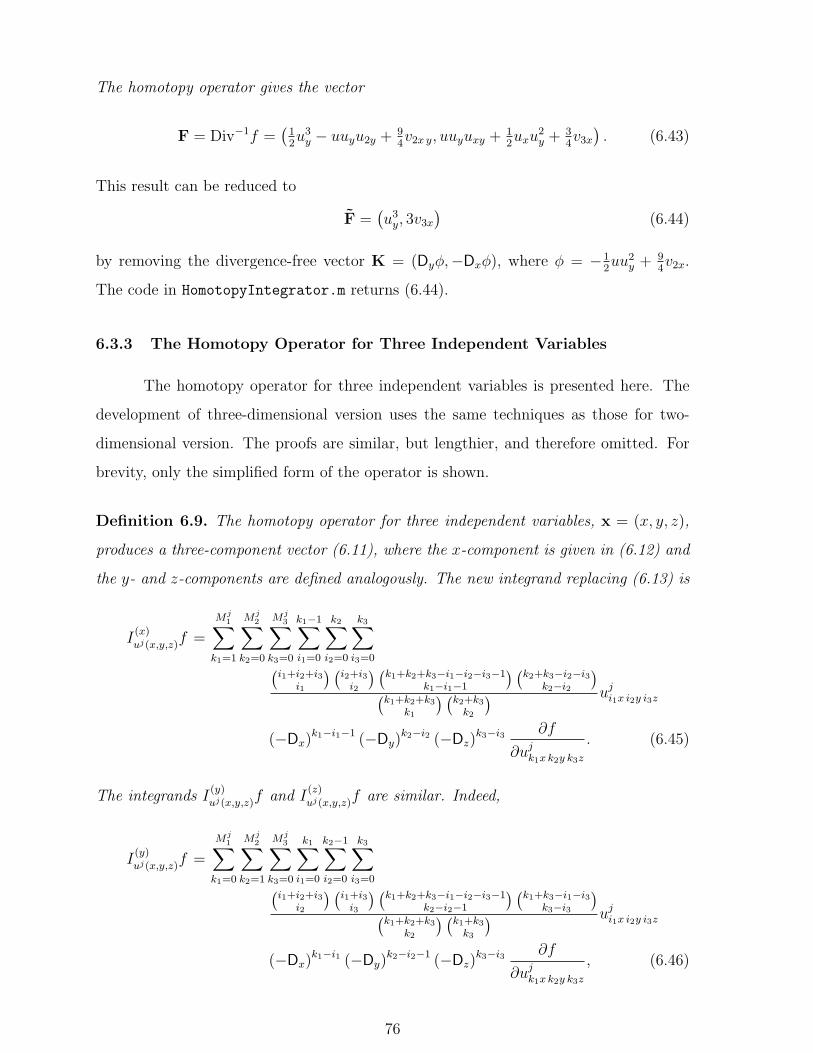
The homotopy operator gives the vector

F = Div−1f =(

12u3y − uuyu2y + 9

4v2x y, uuyuxy + 1

2uxu

2y + 3

4v3x

). (6.43)

This result can be reduced to

F =(u3y, 3v3x

)(6.44)

by removing the divergence-free vector K = (Dyφ,−Dxφ), where φ = −12uu2

y + 94v2x.

The code in HomotopyIntegrator.m returns (6.44).

6.3.3 The Homotopy Operator for Three Independent Variables

The homotopy operator for three independent variables is presented here. The

development of three-dimensional version uses the same techniques as those for two-

dimensional version. The proofs are similar, but lengthier, and therefore omitted. For

brevity, only the simplified form of the operator is shown.

Definition 6.9. The homotopy operator for three independent variables, x = (x, y, z),

produces a three-component vector (6.11), where the x-component is given in (6.12) and

the y- and z-components are defined analogously. The new integrand replacing (6.13) is

I(x)

uj(x,y,z)f =

Mj1∑

k1=1

Mj2∑

k2=0

Mj3∑

k3=0

k1−1∑i1=0

k2∑i2=0

k3∑i3=0(

i1+i2+i3i1

) (i2+i3i2

) (k1+k2+k3−i1−i2−i3−1

k1−i1−1

) (k2+k3−i2−i3

k2−i2

)(k1+k2+k3

k1

) (k2+k3k2

) uji1x i2y i3z

(−Dx)k1−i1−1 (−Dy)

k2−i2 (−Dz)k3−i3 ∂f

∂ujk1x k2y k3z. (6.45)

The integrands I(y)

uj(x,y,z)f and I

(z)

uj(x,y,z)f are similar. Indeed,

I(y)

uj(x,y,z)f =

Mj1∑

k1=0

Mj2∑

k2=1

Mj3∑

k3=0

k1∑i1=0

k2−1∑i2=0

k3∑i3=0(

i1+i2+i3i2

) (i1+i3i3

) (k1+k2+k3−i1−i2−i3−1

k2−i2−1

) (k1+k3−i1−i3

k3−i3

)(k1+k2+k3

k2

) (k1+k3k3

) uji1x i2y i3z

(−Dx)k1−i1 (−Dy)

k2−i2−1 (−Dz)k3−i3 ∂f

∂ujk1x k2y k3z, (6.46)

76

and

I(z)

uj(x,y,z)f =

Mj1∑

k1=0

Mj2∑

k2=0

Mj3∑

k3=1

k1∑i1=0

k2∑i2=0

k3−1∑i3=0(

i1+i2+i3i3

) (i1+i2i1

) (k1+k2+k3−i1−i2−i3−1

k3−i3−1

) (k1+k2−i1−i2

k1−i1

)(k1+k2+k3

k3

) (k1+k2k1

) uji1x i2y i3z

(−Dx)k1−i1 (−Dy)

k2−i2 (−Dz)k3−i3−1 ∂f

∂ujk1x k2y k3z. (6.47)

The three-dimensional version has also been extensively tested. The results were

similar to those for the one- and two-dimensional versions. Expression swell is more pro-

nounced as the number of independent variables increases. In contrast to the integrands

that were expressed in terms of higher-Euler operators, the new integrands, (6.45),

(6.46), and (6.47), largely prevent unwieldy expression swell. The three-dimensional

version also produces a result containing a divergence-free vector, ∇ ×K, where K is

an arbitrary differential vector function. Again, the vector ∇×K needs to be removed

from the result.

6.4 Removing Divergence-Free Terms

As mentioned in the previous section, the homotopy operator acting on exact

expressions with more than one independent variable will produce a vector result that

often contains a divergence-free (curl) vector. For a particular expression, the choice

for divergence-free vectors is infinite. The homotopy operator computes one choice for

that expression and will consistently reproduce the divergence-free vector. A result

containing a divergence-free vector can be of unmanageable size, whereas the result

without the divergence-free part is generally concise.

Several methods exist to remove divergence-free vectors. To do this by hand

requires educated guesses as to what the divergence-free piece contains, a process difficult

to program. The method implemented in HomotopyIntegrator.m uses linear algebra.

Indeed, all it requires is the solution of a linear system which is efficient and easy to

program.

The method for removing curl terms will be explained using (6.43), the result

from Example 6.6. To begin with, attach undetermined coefficients, k1, . . . , kp, to the

77

terms of (6.43) and call the new vector F. This gives

F =

12k1u

3y − k2uuyu2y + 9

4k3v2xy

k4uuyuxy + 12k5uxu

2y + 3

4k6v3x

. (6.48)

Apply the divergence operator (2.5) to both (6.43) and (6.48), producing two corre-

sponding divergences,

f = Div F

= 3u2yuxy + 3v3x y (6.49)

and

f = Div F

= 32k1u

2yuxy − k2uxuyu2y − k2uuxyu2y − k2uuyux2y + 9

4k3v3xy + k4u

2yuxy

+ k4uuxyu2y + k4uuyux2y + 12k5u

2yuxy + k5uxuyu2y + 3

4k6v3xy

=(

32k1 + k4 + 1

2k5

)u2yuxy + (k5 − k2)uxuyu2y + (k4 − k2)uuxyu2y

+ (k4 − k2)uuyux2y +(

94k3 + 3

4k6

)v3xy. (6.50)

Since F and F differ only by a curl vector, their divergences are equal, that is, f must

equal f . Gathering like terms in (6.49) and (6.50) produces the linear system

12(3k1 + 2k4 + k5) = 3,

k5 − k2 = 0,

k4 − k2 = 0,

34(3k3 + k6) = 3.

(6.51)

Removing the divergence-free vector from F can be tricky. It is possible to

remove only part of the divergence-free vector, leaving a divergence-free part behind.

Furthermore, there may be more that one choice for the vector that completely removes

the divergence-free part. Thus, the manner in which the system is solved becomes

important.

Mathematica’s Solve function solves a system of equations working through a

list of variables in order. It takes the first variable in a list and will either find a specific

solution, or it will solve for that variable in terms of subsequent variables. If the variable

78

is found to be arbitrary, Solve moves on to the next variable in the list and does not

report the arbitrary variable. If Solve is given the list k1, . . . , k6, the solution to the

system (6.51) is

k1 = 2− k5, k2 = k5, k3 = 43− 1

3k6, k4 = k5, (6.52)

where k5 and k6 are arbitrary. Since it is desirable to eliminate as many terms as

possible, choose k5 = 0 and k6 = 0. With this choice, k1 = 2, k2 = 0, k3 = 43, and

k4 = 0. Substituting this solution into (6.48) produces the vector

F =(u3y + 3v3x, 0

), (6.53)

a simpler form, but perhaps not the most desirable result.

To find the solution to the system of undetermined coefficients that will produce

a result without any divergence-free part, take the coefficients, ki, from the equations

where the right-hand side is not zero and place them in the list of variables for Solve

first, then add all other coefficients. From the system (6.51), k1, k3, and k6 are placed

at the front of the list, and the rest are added to get k1, k3, k6, k2, k4, k5, which is the

order that Solve will use. The coefficients k1, k3, and k6 are taken first because they

are coefficients of terms that must be in the divergence. For this simple case, the solution

to the system produces the result in (6.53).

Reversing the order of the ki may change the divergence-free result by moving

a term that has mixed partial derivatives to a different component, possibly leading

to a more desirable result. For the system (6.51), if the list for Solve is ordered as

k6, k3, k1, k2, k4, k5, the solution is

k6 = 4− 3k3, k1 = 2− k5, k2 = k5, k4 = k5, (6.54)

with k3 and k5 arbitrary. Since k3 and k5 are free, set them equal to zero. This gives k1 =

2, k2 = 0, k4 = 0, and k6 = 4. Replacing all ki in (6.48) with these solutions produces

(6.44), the simplest possible vector that can be found with balanced components.

The reduction algorithm in HomotopyIntegrator.m has been tested extensively

on both two and three independent variable vector functions. By placing the constants

into the solve list in the correct order, the algorithm runs quickly and returns the sim-

plest possible vector, even when thousands of terms are involved. The next example

79

shows a simple three-dimensional case for which the homotopy operator returns a large

divergence-free term.

Example 6.7. Let u = (u, v), and let

F(x, y, z,u(7)(x, y, z)) =(u2y3z − vuxy, u3ux6y, v

2y − uv5x2z

). (6.55)

Applied to f = DivF, the homotopy operator produces a vector with 42 terms in the

x-component, 36 terms in the y-component, and 32 terms in the z-component. The

reduction algorithm is able to return (6.55) using 0.25 seconds of CPU time. When f is

given to HomotopyIntegrator.m, the program will return (6.55).

6.5 Limitations of the Homotopy Operator

The homotopy operator has proven to be quite versatile in tests using a wide

variety of functions. However, there are two possible limitations to its use. When

either one is encountered, it may be necessary to pursue another avenue to complete the

integration.

One advantage of the homotopy operator is that it replaces an integration by

parts problem on a function with one independent variable with an integration over an

auxiliary variable that can often be done using direct methods. In multi-variable cases,

the integration over the auxiliary variable replaces a possible integration over multiple

variables. It is possible, however, that if the given expression is a complex composition

of functions, even the integral for the auxiliary variable may be too complex to integrate.

The code HomotopyIntegrator.m will print a message when this happens.

The second limitation occurs with exact expressions in rational form. If a function

f(x,u(M)(x)) is rational and f is in the kernel of the degree operator, M, then the

homotopy operators as defined in Definitions 6.5, 6.7, and 6.9 will not work, as discussed

in Case 3 of the proof for Theorem 6.1. Consider the one-dimensional case. In Theorem

6.3, it was shown that if f is an exact differential function, then

Mf = Dx

N∑j=1

(Iuj(x)f), (6.56)

for dependent variable uj. When f ∈ Ker M, that is, when Mf = 0, thenn∑j=1

Iuj(x)f = C,

C ∈ R, so the homotopy operator will return a constant.

80

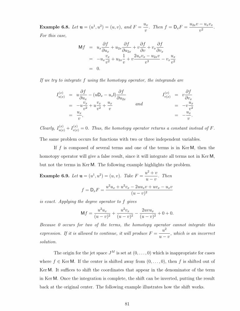
Example 6.8. Let u = (u1, u2) = (u, v), and F =uxv

. Then f = DxF =u2xv − uxvx

v2.

For this case,

Mf = ux∂f

∂ux+ u2x

∂f

∂u2x

+ v∂f

∂v+ vx

∂f

∂vx

= −uxvxv2

+ u2x1

v+ v

2uxvx − u2xv

v3− vx

uxv2

= 0.

If we try to integrate f using the homotopy operator, the integrands are

I(x)u(x) = u

∂f

∂ux− (uDx − uxI)

∂f

∂u2x

= −uvxv2

+ uvxv2

+uxv

=uxv,

and

I(x)v(x) = v

∂f

∂vx

= −vuxv2

= −uxv.

Clearly, I(x)u(x) + I

(x)v(x) = 0. Thus, the homotopy operator returns a constant instead of F .

The same problem occurs for functions with two or three independent variables.

If f is composed of several terms and one of the terms is in Ker M, then the

homotopy operator will give a false result, since it will integrate all terms not in Ker M,

but not the terms in Ker M. The following example highlights the problem.

Example 6.9. Let u = (u1, u2) = (u, v). Take F =u2 + v

u− v. Then

f = DxF =u2ux + u2vx − 2uuxv + uvx − uxv

(u− v)2

is exact. Applying the degree operator to f gives

Mf =u2ux

(u− v)2+

u2vx(u− v)2

− 2uvux(u− v)2

+ 0 + 0.

Because 0 occurs for two of the terms, the homotopy operator cannot integrate this

expression. If it is allowed to continue, it will produce F =u2

u− v, which is an incorrect

solution.

The origin for the jet space JM is set at (0, . . . , 0) which is inappropriate for cases

where f ∈ Ker M. If the center is shifted away from (0, . . . , 0), then f is shifted out of

Ker M. It suffices to shift the coordinates that appear in the denominator of the term

in Ker M. Once the integration is complete, the shift can be inverted, putting the result

back at the original center. The following example illustrates how the shift works.

81

Example 6.10. Let f(x,u(2)(x)) =u2xv − uxvx

v2, where f ∈ Ker M. Since v is in the

denominator, shift v by v0, that is, replace v with v−v0, to get f0 =u2x(v − v0)− uxvx

(v − v0)2.

Using the homotopy operator (6.2) to integrate f0, first compute the integrands (6.16)

to get

I(x)u(x)f0 =

uxv − v0

and I(x)v(x)f0 =

−uxv(v − v0)2

.

Then,

Hu(x)f0 =

∫ 1

0

(ux

v − v0

− uxv

(v − v0)2

)[λu]

dλ

λ

= −∫ 1

0

uxv0

(λv − v0)2dλ

=uxv0

v(λv − v0)

∣∣∣∣10

=ux

v − v0

.

Lastly, remove the shift by replacing v with v + v0 (or simply set v0 = 0) to get

F = Hu(x)f =uxv.

Similar problems occur with rational functions involving multiple independent

variables. Again, a shift of the coordinate(s) in the denominator will solve the problem.

However, the complexity of the integration over the auxiliary variable λ increases rapidly

when there are multiple independent variables. Thus, applying the shifts can cause

HomotopyIntegrator.m to run for a long time.

82

CHAPTER 7

CONSTRUCTION OF CONSERVATION LAWS FOR NONLINEAR PDES

The techniques for constructing conservation laws will be shown by using the

PDEs given in Chapter 3. Each PDE will illustrate various aspects of the computations

used to determine conservation laws. The program ConservationLawsMD.m consists of

algorithms based on these computations.

The procedure begins by computing the density, ρ, in equation (3.5). To do

this, a candidate density is built by constructing lists of terms invariant under the

scaling symmetry of the PDE, then forming an expression by summing the terms after

multiplying each term by an undetermined coefficient. Values for the undetermined

coefficients are found by applying the zeroth-Euler operator (4.2) to the t-derivative of

the candidate density. Once the density is obtained, the flux, J is found by inverting

the divergence on Dt(ρ) using the homotopy operator. In summary, the steps are:

i. Determine a scaling symmetry for the PDE.

ii. Construct a candidate density with undetermined coefficients using the scalingsymmetry.

iii. Calculate the unknown coefficients for the density.

iv. Calculate the flux, once the density is known.

The ZK equation (3.7) is a (2+1)-dimensional example that will be used to il-

lustrate the main steps listed above. The NTGF equation (3.18) is a good (3+1)-

dimensional example to demonstrate how a single candidate density can be split into

several densities. Gardner’s equation (3.35) does not have a scaling symmetry unless

the parameter β is included in the computations for the scaling symmetry.

7.1 Conservation Laws for the Zakharov-Kuznetsov Equation

The (2+1)-dimensional ZK equation,

ut + αuux + β(u2x + u2y)x = 0. (7.1)

83

is taken as the first example because it is one of the few multi-dimensional examples

that is an evolution equation, and it has polynomial conservation laws. Therefore, the

method for computing conservation laws is straightforward. Also, conservation laws for

the ZK equation have been previously studied [40, 68, 83], thus, the results presented in

this section can be easily verified.

7.1.1 Establishing a Scaling Symmetry

Every PDE has a unique set of Lie-point symmetries which can include transla-

tions, rotations, scalings and other symmetries. The Lie-point symmetries are generated

by constructing a set of infinitesimal generators. In turn, this requires solving an over-

determined system of linear partial differential equations which lead to a set of spanning

vector fields that can be translated into symmetry groups [12, 56]. The application of

symmetries allows one to generate additional solutions from known solutions. In this

dissertation, one type of Lie-point symmetry, the scaling or dilation symmetry, will be

used to formulate conservation laws.

A candidate density is formed by assuming that the given PDE is invariant under

a scaling symmetry, one of the Lie-point symmetries.

Definition 7.1. A PDE is scaling invariant when a scaling transformation applied to

the PDE returns the PDE multiplied by a constant factor.

Although not all PDEs will have a scaling symmetry, it is possible to “induce” a scaling

symmetry by introducing one or more parameters into the PDE. A scaling symmetry

can be calculated using linear algebra, which avoids having to solve a system of differ-

ential equations. This is done by constructing a set of weights for every dependent and

independent variable in the PDE. Once the weights are computed, a candidate density

can be built as a linear combination of terms that are scaling invariant for a prescribed

rank [52].

The next example illustrates how the ZK equation (7.1) is invariant under a

particular scaling symmetry. The scaling factor, λ, used in examples in this chapter

should not be confused with the auxiliary variable used in the homotopy operator.

84

Example 7.1. The ZK equation (7.1) is scaling invariant under the scaling symmetry

(t, x, y, u)→ (λ−3t, λ−1x, λ−1y, λ2u), (7.2)

where λ is an arbitrary scaling parameter, different from the λ in the homotopy operator.

It is not necessary to scale the constant parameters, α and β, in (7.1). To verify the

scaling invariance for (7.1), let t = λ−3t, x = λ−1x, y = λ−1y, and u = λ2u. Applying

the scaling symmetry to equation (7.1) transforms the left-hand side of the equation as

follows,

ut + αuux + βu3x + βux2y

= Dtu+ αuDxu+ βD3xu+ βDxD

2yu

= Dtu

λ2+ α

u

λ2Dx

u

λ2+ βD3

x

u

λ2+ βDxD

2y

u

λ2

=1

λ2Dtu(Dtt) +

α

λ4uDxu(Dxx) +

β

λ2D3xu(Dxx)3 +

β

λ2DxD

2yu(Dxx)(Dyy)2

=1

λ2Dtu

(Dt

t

λ3

)+α

λ4uDxu

(Dxx

λ

)+β

λ2D3xu(Dxx

λ

)3

+β

λ2DxD

2yu(Dxx

λ

)(Dyy

λ

)2

=1

λ5

(Dtu+ αuDxu+ βD3

xu+ βDxD2yu)

=1

λ5(ut + αuux + βu3x + βux2y) . (7.3)

The ZK equation is scaling invariant under the scaling symmetry (7.2) since the

system in the scaled variables is identical to (7.1) to within the constant factor, 1λ5 .

Clearly, the transformed PDE (7.3) has the same solutions as the original. Fur-

thermore, the scaling symmetry can be used to find densities, fluxes, generalized sym-

metries, recursion operators, and so on. Focusing on conservation laws, the defining

equations (3.5) must hold on solutions of the PDE. Therefore, ρ and J must obey the

scaling symmetry of the PDE.

To construct a possible density, the scaling symmetry is used to find a weight for

each variable, from which a rank can be found for the PDE.

Definition 7.2. Let λ be an arbitrary scaling parameter. The weight of a variable

(dependent or independent) is defined as the exponent p in the factor λp that multiplies

the variable. For variable x, if the factor is λ−p, the weight is denoted W (x) = −p.

Total derivatives also carry a weight. If W (x) = −p, then W (Dx) = p.

85

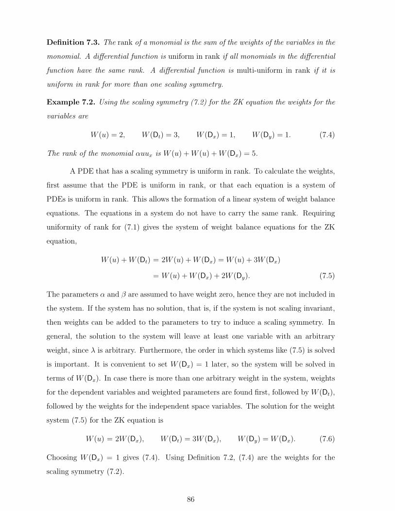
Definition 7.3. The rank of a monomial is the sum of the weights of the variables in the

monomial. A differential function is uniform in rank if all monomials in the differential

function have the same rank. A differential function is multi-uniform in rank if it is

uniform in rank for more than one scaling symmetry.

Example 7.2. Using the scaling symmetry (7.2) for the ZK equation the weights for the

variables are

W (u) = 2, W (Dt) = 3, W (Dx) = 1, W (Dy) = 1. (7.4)

The rank of the monomial αuux is W (u) +W (u) +W (Dx) = 5.

A PDE that has a scaling symmetry is uniform in rank. To calculate the weights,

first assume that the PDE is uniform in rank, or that each equation is a system of

PDEs is uniform in rank. This allows the formation of a linear system of weight balance

equations. The equations in a system do not have to carry the same rank. Requiring

uniformity of rank for (7.1) gives the system of weight balance equations for the ZK

equation,

W (u) +W (Dt) = 2W (u) +W (Dx) = W (u) + 3W (Dx)

= W (u) +W (Dx) + 2W (Dy). (7.5)

The parameters α and β are assumed to have weight zero, hence they are not included in

the system. If the system has no solution, that is, if the system is not scaling invariant,

then weights can be added to the parameters to try to induce a scaling symmetry. In

general, the solution to the system will leave at least one variable with an arbitrary

weight, since λ is arbitrary. Furthermore, the order in which systems like (7.5) is solved

is important. It is convenient to set W (Dx) = 1 later, so the system will be solved in

terms of W (Dx). In case there is more than one arbitrary weight in the system, weights

for the dependent variables and weighted parameters are found first, followed by W (Dt),

followed by the weights for the independent space variables. The solution for the weight

system (7.5) for the ZK equation is

W (u) = 2W (Dx), W (Dt) = 3W (Dx), W (Dy) = W (Dx). (7.6)

Choosing W (Dx) = 1 gives (7.4). Using Definition 7.2, (7.4) are the weights for the

scaling symmetry (7.2).

86

The choice W (Dx) = 1 is convenient, but it is possible that W (Dx) may have

to be assigned a different value. When formulating the candidate density the weights

of the dependent variables, weighted parameters, and total derivatives of independent

variables must be positive. Thus, the choice for W (Dx) may depend on the values of the

other weights. The weights do not have to be integer values.

7.1.2 Construction of a Candidate Density

Once the scaling symmetry is established, the terms of a candidate density can

be constructed by fixing a value for the rank and combining dependent variables, partial

derivatives on dependent variables, and independent variables into monomials so that

each monomial has that preselected rank. Linearly combining these monomials with

undetermined coefficients, the density in its final form will have a rank equal to the rank

initially chosen. A candidate density for the ZK equation (7.1) with a rank of 6 will be

constructed as the steps are explained.

First, construct a list P containing all powers of dependent variables and products

of dependent variables that have rank 6 or less, where 6 is the rank chosen for the

candidate density.

Example 7.3. For the ZK equation (7.1), using the weights (7.4), all possible powers

and products of dependent variables with rank 6 or less are

P = u3, u2, u. (7.7)

Second, construct a new list, Q, by first taking all terms in P with a rank of 6

and placing them into Q. For all terms left in P adjust their ranks up to rank 6 by

applying total derivatives with respect to the independent space variables, then place

the results in Q. There may be several choices for adjusting the rank of the term and

all of these choices should be added to Q. When moving terms into Q, all numerical

coefficients can be ignored as they will be recalculated later.

Example 7.4. In P (7.3), the term u3 has rank 6, so it is moved directly into Q. The

term u2 has rank 4 and can be adjusted to rank 6 by applying Dx twice, by applying Dy

twice, and by applying each of Dx and Dy once. Each time a total derivative is applied

87

to u2, the rank of the term increases by 1 since the weight for each total derivative is 1,

by (7.5). The term u has rank 2 and can be adjusted to rank six in five ways. List Q is

Q = u3, u2x, uu2x, u

2y, uu2y, uxuy, uuxy, u4x, u3xy, u2x2y, ux3y, u4y. (7.8)

All twelve terms in Q have rank 6.

Third, from Q, remove all terms that are divergences or divergent-equivalent (see

Definitions 5.1 and 5.2). If these terms belong in the conservation law, they will occur

in the flux. If they are left in the candidate density, the final form for the density would

be a linear combination of equivalent and/or trivial densities. Once all divergences and

divergence-equivalent terms have been removed from Q, put the remaining terms in list

R. Use Algorithm 5.1 to find divergences and divergence equivalent terms.

Example 7.5. Apply the zeroth-Euler operator (4.4) to Q in (7.8) term by term to get

Lu(x,y)Q = 3u2,−2u2x, 2u2x,−2u2y, 2u2y,−2uxy, 2uxy, 0, 0, 0, 0, 0. (7.9)

Divergences are terms corresponding to 0 in Lu(x,y)Q, so u4x, u3xy, u2x2y, ux3y, and u4y

can be removed from Q. Next, attach undetermined coefficients to each term in (7.9),

then set the sum of these terms equal to zero,

3p1u2 − 2p2u2x + 2p3u2x − 2p4u2y,+2p5u2y − 2p6uxy + 2p7uxy = 0.

After gathering like terms and forming a system of coefficient equations, the following

relationships are found among the undetermined coefficients,

p1 = 0, p2 = p3, p4 = p5, p6 = p7.

Thus, the terms with coefficients p3, p5, and p7 are divergence-equivalent to the terms

with coefficients p2, p4, and p6, respectively. For each divergence-equivalent pair, the

terms with the highest order are removed from Q in (7.8).

This leaves

R = u3, u2x, u

2y, uxuy, (7.10)

which contains the terms left in Q after all divergences and divergence-equivalent terms

have been removed.

88

The candidate density is constructed by putting an undetermined coefficient, ci,

on each term in R and adding all of the terms, that is, linearly combining the terms in

R, to create the expression

ρ1 = c1u3 + c2u

2x + c3u

2y + c4uxuy. (7.11)

ρ1 is a candidate density of rank 6 for the ZK equation. The next step is to determine

values for the ci, which is done in the next section.

In the next example, following the steps used to construct (7.11), a second candi-

date density of rank 1 containing terms which are products of independent and dependent

variables will be constructed for the ZK equation (7.1).

Example 7.6. The candidate density for rank 1 will have independent variables of degree

1 multiplied explicitly to the dependent variables. Since W (Dx) = 1,W (Dy) = 1, and

W (Dt) = 3 by (7.4), W (x) = −1,W (y) = −1, and W (t) = −3, respectively, as described

in Definition 7.2. First, find all powers and products of dependent variables with rank

1 or less. In this case, there are none, so P = . To find all terms with explicit

independent variable x, find all polynomial terms of rank 2 or less, then multiply each

term by x. This creates the list P(x) with terms of rank 1 or less,

P(x) = xu.

Since W (y) = −1, find all polynomial terms of rank 2 or less, then multiply each term

by y to create the rank 1 list,

P(y) = yu.

The last set of terms is found by multiplying t to all polynomial terms of rank 4 or less,

giving

P(t) = tu2, tu

In the construction of a the candidate density, t is a parameter. By keeping t a parameter,

the possibility of constructing trivial conservation laws is eliminated. Bring all terms in

P, P(x), P(y), and P(t) up to rank 1 by applying Dx and Dy, then combine the lists to get

Q = xu, yu, tu2, tu2x, tuxy, tu2y.

89

Remove any divergences and divergent-equivalent terms from Q to get

R = xu, yu, tu2.

A second candidate density for the ZK equation is

ρ2 = c1xu+ c2yu+ c3tu2. (7.12)

Note that it is necessary to set an upper bound for the degree of x, y, and t,

otherwise ρ2 would have an infinite number of terms, all of rank 1. In this case, a degree

of 1 is sufficient to find all rank 1 densities.

7.1.3 Determination of the Actual Density

All, part, or none of the candidate density may be an actual density for a PDE.

Indeed, the candidate density may be trivial or a linear combination of two or more

independent densities. Analysis of the candidate density is done using the continuity

equation (3.5). By (3.5), Dtρ = −Div J, so Dtρ must be a divergence with respect to

the space variables. If the PDE is an evolution equation written in the form (3.1), all

t-derivatives can be replaced with the right-hand side of the evolution equation. The

next example shows Dtρ1 for candidate density (7.11) of rank 6 after all t-derivatives

have been replaced.

Example 7.7. Using (2.4), the total t-derivative of the rank 6 candidate density (7.11)

is

Dtρ1 = 3c1u2ut + 2c2uxutx + 2c3uyuty + c4(utxuy + uxuty).

Let E1 be −Dtρ1 where all ut in Dtρ1 have been replaced by the right-hand side of the

ZK equation (5.12). Thus

E1 = 3c1u2(αuux + β(u3x + ux2y)) + 2c2ux(αuux + β(u3x + ux2y))x

+ 2c3uy(αuux + β(u3x + ux2y))y + c4(uy(αuux + β(u3x + ux2y))x

+ ux(αuux + β(u3x + ux2y))y). (7.13)

Since Dtρ1 is required to be a divergence, the zeroth-Euler operator (4.4) applied

to E1 must be 0 by Theorem 4.1. This forms an equation where the coefficients on like

terms must add up to zero. Thus, a linear system of equations is obtained, making it

possible to compute values for the undetermined coefficients using linear algebra.

90

Example 7.8. Applying the zeroth-Euler operator to (7.13) gives

0 ≡ Lu(x,y) E1

= −2((3c1β + c3α)uxu2y + 2(3c1β + c3α)uyuxy + 2c4αuxuxy + c4αuyu2x

+ 3(3c1β + c2α)uxu2x

).

A linear system of equations for the undetermined coefficients is formed by setting each

factor equal to zero. After eliminating duplicate equations, the system is

3c1β + c3α = 0, c4α = 0, 3c1β + c2α = 0. (7.14)

Note that this system is parameterized by the parameters α and β, appearing

in the PDE. Before solving the system (7.14), it is necessary to compute compatibility

conditions on the parameters α and β, if any exist, assuming that the parameters are

nonzero. A detailed algorithm for computing the compatibility conditions is given in [30].

If a compatibility condition exists, but is ignored, then the solutions for all ci in (7.14)

will be zero which means there is no density. Before computing compatibility conditions,

from the system of coefficient equations remove all equations where the solution for the

ci must be zero. Next, take all remaining ci in the system of coefficient equations, and

set them equal to 1, one at a time, then algebraically eliminate all other ci.

Example 7.9. To check for compatibility conditions on the parameters in (7.14), first

remove c4α = 0 from the system since clearly c4 = 0 which means that the term with

coefficient c4 in the candidate density (7.11) is not part of the actual density. For the

remaining equations

3c1β + c3α = 0, 3c1β + c2α = 0, (7.15)

set c1 = 1 and algebraically eliminate c2 and c3 from (7.15). With c2 = c3 = −3βα

, all

equations in the system are satisfied. Next set c2 = 1 and algebraically eliminate c1 and

c3 from (7.15). With c1 = − α3β

and c3 = 1, the system is solved. Finally, set c3 = 1

and algebraically eliminate c1 and c2 from (7.15). With c1 = − α3β

and c2 = 1, again, the

system is solved.

Each time a ci is set equal to one, the term with that coefficient is forced to remain

in the density while the parameters are evaluated. If the candidate density is a linear

91

combination of densities, more than one compatibility condition could occur, so it is

necessary to check each term in the density.

There are three possible outcomes when a particular ck = 1 and all other ci are

eliminated.

Outcome 1: All remaining ci are eliminated from the system leaving only identities.

There are no compatibility conditions on the parameters.

Outcome 2: All remaining ci are eliminated from the system leaving a new consis-

tent system of equations containing parameters only. The solution to

this new system provides the compatibility conditions on the parame-

ters.

Outcome 3: All remaining ci are eliminated from the system leaving a new system of

equations containing parameters only. This new system either requires

one of the parameters to be zero, or is inconsistent. In either case, the

particular ck set equal to 1 must actually be zero.

The compatibility check for candidate density (7.11) in Example 7.9 has Outcome 1;

there are no compatibility conditions.

Once the compatibility conditions are known, it is possible to find a solution to

the system of coefficient equations.

Example 7.10. The solution to (7.14) is

c2 = −3βαc1, c3 = −3β

αc1, c4 = 0, (7.16)

where c1 is arbitrary. This solution yields the density

ρ1 = c1u3 − c1

3βαu2x − c1

3βαu2y.

Since c1 is arbitrary, set c1 = 1 to get

ρ1 = u3 − 3βα

(u2x + u2

y), (7.17)

the density given in conservation law (3.11).

The next example shows a complete set of computations for the undetermined

coefficients for candidate density (7.12) of rank 1.

92

Example 7.11. First, apply the total t-derivative to the candidate density (7.12) for

rank 1 to get

Dtρ2 = c1xut + c2yut + c3u2 + 2c3tuut.

Let E2 be −Dtρ2 where all ut in Dtρ2 have been replaced by the right-hand side of the

ZK equation (5.12). Thus

E2 = c1x(αuux + β(u3x + ux2y)) + c2y(αuux + β(u3x + ux2y))− c3u2

+ 2c3tu(αuux + β(u3x + ux2y)). (7.18)

Require E2 to be a divergence. Hence,

0 ≡ Lu(x,y) E2

= −(αc1 + 2c3)u.

There is only one equation which does not generate any compatibility conditions on the

parameters α and β. The solution for this equation is

c1 = − 2αc3, (7.19)

where c3 is arbitrary. This leads to the density

ρ2 = c2yu+ c3tu2 − 2

αc3xu. (7.20)

where c2 and c3 are arbitrary.

The presence of two arbitrary coefficients indicates that ρ2 consists of two inde-

pendent densities. However, Example 5.6 shows that the conservation law with density

yu is equivalent to the ZK equation (3.9), which is obtained at rank 2. Thus, by taking

c3 = 1, the only new density is

ρ2 = tu2 − 2αxu. (7.21)

This is the density for conservation law (3.12).

7.1.4 Calculation of the Flux

Once a density has been found, the corresponding flux can be calculated by

using the homotopy operator (6.5) with integrands (6.32) and (6.33), since by (3.5),

93

J = Div−1 (−Dtρ). The undetermined coefficients for each density were calculated so

that E1 (7.13) and E2 (7.18) are exact. Thus all that is needed is to replace the ci in E1

and E2 using the solutions for the undetermined coefficients, then apply the homotopy

operator.

Example 7.12. For ρ1, (7.17), E1 = −Dtρ1 is (7.13) with the solutions (7.16) and

c1 = 1 replacing all ci so that

E1 = 3u2(αuux + β(u3x + ux2y))− 6βαux(αuux + β(u3x + ux2y))x

− 6βαuy(αuux + β(u3x + ux2y))y.

Now, to find the flux, apply the homotopy operator to E1,

J1 =(H(x)

u(x,y)E1,H(y)u(x,y)E1

)=(

34αu4 + βu2(3u2x + 2u2y)− βu(6u2

x + 2u2y) + 3β2

4αu(u2x2y + u4y)

− β2

αux(

72ux2y + 6u3x)− β2

αuy(4u2xy + 3

2u3y) + β2

α(3u2

2x + 52u2xy + 3

4u2

2y)

+ 5β2

4αu2xu2y, βu

2uxy − 4βuuxuy − 3β2

4αu(ux3y + u3xy)− β2

4αux(13u2xy + 3u3y)

− 5β2

4αuy(u3x + 3ux2y) + 9β2

4αuxy(u2x + u2y)

). (7.22)

After removing the divergence-free term K = (Dyθ,−Dxθ) with

θ = 2βu2uy + 3β2

4αu(u2xy + u3y) + 5β2

2αuxuxy + 15β2

4αuyu2y + 5β2

4αu2xuy,

J1 −K is the flux given in conservation law (3.11).

The flux corresponding to the rank 1 density (7.21) is found in the same manner.

Example 7.13. For ρ2 (7.21), E2 = −Dtρ2 is (7.18) with c1 = − 2α

, c2 = 0, and c3 = 1,

E2 = − 2αx(αuux + β(u3x + ux2y))− u2 + 2tu(αuux + β(u3x + ux2y)). (7.23)

Again, to find the flux, apply the homotopy operator to E2. After removing the small

divergence-free term, the flux is the same as in conservation law (3.12).

7.2 Conservation Laws for the Non-stationary Transonic Gas Flow Equation

The NTGF equation (3.18) serves as a good model for the computation of con-

servation laws in (3+1)-dimensions. The construction of two polynomial conservation

laws, (3.21) and (3.22), will be shown in this section.

94

Unlike the ZK equation, the NTGF equation is not an evolution equation. The

transformation of the NTGF equation into two evolution equations was shown in Ex-

ample 3.1. The evolution equations used for calculations in this section are

ut = v,

vt = 2uxz + uxu2x − u2y.(7.24)

The reader should be aware that with the interchange of t and z in the transformation,

the densities being calculated are actually the z-component of the flux in (3.21) and

(3.22). All calculations that follow are based on (7.24).

7.2.1 Scaling Symmetry for the NTGF Equation

The system of weight equations for (7.24) is

W (v) = W (u) +W (Dt),

W (v) +W (Dt) = W (u) +W (Dx) +W (Dz) = 2W (u) + 3W (Dx)

= W (u) + 2W (Dy). (7.25)

The weight system has to be solved in terms of W (Dx) and W (Dy), thus, there are two

free weights

W (u) = 2W (Dy)− 3W (Dx), W (v) = 3W (Dy)− 3W (Dx),

W (Dz) = 2W (y)−W (Dx), W (Dt) = W (Dy).(7.26)

Taking W (Dx) = 1 and W (Dy) = a, the scaling symmetry for (7.24) is.

(x, y, z, t, u, v) −→ (λ−1x, λ−ay, λ1−2az, λ−at, λ2a−3u, λ3a−3v), (7.27)

where a is arbitrary. In this case, there is a one-parameter family of scaling symmetries.

For example, setting a = 2 produces the symmetry

(x, y, z, t, u, v) −→ (λ−1x, λ−2y, λ−3z, λ−2t, λu, λ3v), (7.28)

whereas setting a = 3 produces the symmetry

(x, y, z, t, u, v) −→ (λ−1x, λ−3y, λ−5z, λ−3t, λ3u, λ6v).

95

Weights do not have to be integers. For example, setting a = 52

produces the symmetry

(x, y, z, t, u, v) −→ (λ−1x, λ−5/2y, λ−4z, λ−5/2t, λ2u, λ9/2v).

All three symmetries are valid choices under the conditions set in Section 7.1.1,

hence by Definition 7.3, the NTGF equation is multi-uniform in rank. The symmetry

(7.28) will be used to find a candidate density, with the weights,

W (u) = 1, W (v) = 3, W (Dt) = 2, W (Dx) = 1, W (Dy) = 2, W (Dz) = 3.

(7.29)

7.2.2 Construction of Candidate Densities

Since the NTGF evolution equations are multi-uniform in rank, a candidate den-

sity for a particular rank can be split further by using additional symmetries in the

family. The procedure will be shown by calculating all polynomial candidate densities

at rank 6 for (7.24) using (7.29).

First, it is necessary to find lists P , Q, and R following the steps described in

Section 7.1.2.

Example 7.14. Using the weights (7.29), the list of all combinations of dependent

variables of rank 6 or less is

P = u6, u3v, v2, u5, u2v, u4, uv, u3, v, u2, u.

Bringing all terms up to rank 6 by applying Dx, Dy, and Dz gives the list

Q = u6, u3v, v2, u4ux, u2vx, uuxv, u

2u2x, u

3u2x, u3uy, uxvx, u2xv, uv2x, uyv, uvy, u

3x,

uuxu2x, u2u3x, uuxuy, u

2uxy, u2uz, v3x, vxy, vz, u

22x, uxu3x, uu4x, uxuxy, u2xuy,

uu2xy, uxuz, uuxz, u2y, uu2y, u5x, u3xy, ux2y, u2xz. (7.30)

Use Algorithm 5.1 to remove all divergences and divergence-equivalent terms. First,

96

apply the zeroth-Euler operator (4.5) to every term in (7.30),

Lu(x,y,z)Q =

(6u5, 0), (3u2v, u3), (0, 2v), (0, 0), (2uvx,−2uux), (−uvx, uux),

(−2u(u2x + uu2x), 0), (6u(u2

x + uu2x), 0), (0, 0), (−v2x,−u2x), (v2x, u2x),

(v2x, u2x), (−vy, uy), (vy,−uy), (−6uxu2x, 0), (3uxu2x, 0), (−6uxu2x, 0),

(−uxuy − 2uuxy, 0), (2(uxuy − 2uuxy), 0), (0, 0), (0, 0), (0, 0), (0, 0),

(2u4x, 0), (−2u4x, 0), (2u4x, 0), (0, 0), (0, 0), (0, 0), (−2uxz, 0),

(2uxz, 0), (−2u2y, 0), (2u2y, 0), (0, 0), (0, 0), (0, 0), (0, 0), (7.31)

where the variational derivatives correspond to each term in Q. The terms u4ux, u3uy,

u2uz, v3x, vxy, vz, uxuxy, u2xuy, uu2xy, u5x, u3xy, ux2y, and u2xz are divergences. A

linear combination of the terms in (7.31) set equal to (0, 0) yields(6p1u

5 + 3p2u2v + (2p5 − p6)uvx − (2p7 − 6p8)u(u2

x + uu2x)− (p10 − p11 − p12)v2x

− (p13 − p14)vy − (6p15 − 3p16 + 6p17)uxu2x − (p18 − 2p19)(uxuy + 2uuxy)

+ (2p24 − 2p25 + 2p26)u4x − (2p30 − 2p31)uxz − (2p32 − 2p33)u2y, p2u3 + 2p3v

+ (2p5 − p6)uux − (p10 − p11 − p12)u2x + (p13 − p14)uy)

=(0, 0), (7.32)

where the subscript on each undetermined coefficient matches the position of the vari-

ational derivative in Q. In (7.32), clearly p1 = p2 = p3 = 0, p5 = 12p6, p7 = 3p8,

p10 = p11 + p12, p13 = p14, p15 = 12p16 − p17, p18 = 2p19, p24 = p25 − p26, p30 = p31 and

p32 = p33, where p6, p9, p11, p12, p14, p16, p17, p19, p25, p26, p31, and p33 are arbitrary.

Each solution in terms of some pi represents a pair or triplet of divergence-equivalent

terms. All terms whose position in Q is the same as the subscript on the arbitrary pi

are divergence-equivalent terms that can be removed from Q. The terms left in Q form

R = u6, u3v, v2, u2vx, u2u2

x, uxvx, uyv, u3x, uuxuy, u

22x, uxuz, u

2y. (7.33)

The terms in R will be used to construct candidate densities.

Since the scaling symmetry (7.27) is multi-uniform in rank, R can be subdivided.

With W (Dx) = 1 and W (Dy) = a, the weight equations (7.26) become

W (u) = 2a− 3 W (v) = 3a− 3, W (Dz) = 2a− 1, W (Dt) = a. (7.34)

97

The weights in (7.34) can be used to calculate symbolic ranks for each term in R. For

example, the symbolic rank for u3v is

W (u3v) = 3W (u) +W (v)

= 3(2a− 3) + 3a− 3

= 9a− 12.

Terms with the same symbolic rank will be grouped together to form a candidate density.

Several candidate densities can be formed, one for each symbolic rank.

Example 7.15. After the symbolic ranks have been calculated for all terms in R, seven

candidate densities can be formed. Table 7.1 lists the symbolic ranks paired with terms

that carry that symbolic rank. Candidate densities are shown for each symbolic rank.

Table 7.1: Candidate densities for the non-stationary transonic gas flow equation.

Symbolic Terms From R With Candidate DensityRank This Symbolic Rank

4a− 2 u22x ρ1 = c1u

22x

5a− 4 uxvx ρ2 = c1uxvx

6a− 6 v2, u3x, uxuz, uyv, u

2y ρ3 = c1v

2 + c2u3x + c3uxuz + c4uyv + c5u

2y

7a− 8 u2vx, uuxuy ρ4 = c1u2vx + c2uuxuy

8a− 10 u2u2x ρ5 = c1u

2u2x

9a− 12 u3v ρ6 = c1u3v

12a− 18 u6 ρ7 = c1u6

7.2.3 Determination of the Actual Densities

Each candidate density in Table 7.1 must be evaluated separately, however, each

candidate density contains only a few terms and is easy to evaluate. Densities ρ1 and

ρ3 will be evaluated in detail in the following examples. The procedure is the same as

that used for the ZK equation.

Example 7.16. Applying the Dt operator (2.4) to ρ1 in Table 7.1 gives

Dtρ1 = 2c1u2xut2x.

98

Use (7.24) to replace ut with v so that

Dtρ1 = 2c1u2xv2x.

Next, require Dtρ1 to be a divergence which implies that the zeroth-Euler operator acting

on Dtρ1 must be (0, 0). This gives the equation

Lu(x,y) (Dtρ1) = (2c1v4x, 2c1u4x) ≡ (0, 0).

The system of undetermined coefficients has only one equation, 2c1 = 0. Since c1 = 0,

candidate ρ1 does not form a density.

Similar results occur for candidate densities ρ2, ρ4, ρ5, ρ6, and ρ7. None of these

candidates form a density. Next, evaluate ρ3.

Example 7.17. The total t-derivative (2.4) of ρ3 in Table 7.1 gives

Dtρ3 = 2c1vvt + 3c2u2xutx + c3utxuz + c3uxutz + c4uyvt + c4utyv + 2c5uyuty.

Set E3 = −Dtρ3 and use (7.24) to replace ut with v and vt with 2uxz +uxu2x−u2y to get

E3 = −2c1v(2uxz + uxu2x − u2y)− 3c2u2xvx − c3(vxuz + uxvz)

− c4uy(2uxz + uxu2x − u2y)− c4vyv − 2c5uyvy. (7.35)

Next, the zeroth-Euler operator is applied to E3, and the result is set equal to zero,

yielding

Lu(x,y) E3

=

(3c2 − c1)(uxv2x + u2xvx) + (c3 − 2c1)vxz + (c1 + c5)v2y

(3c2 − c1)uxu2x + (c3 − 2c1)uxz + (c1 + c5)u2y

≡ 0

0

. (7.36)

From (7.36), the system for the undetermined coefficients is

3c2 − c1 = 0, c3 − 2c1 = 0, c1 + c5 = 0. (7.37)

The solution is

c1 = −c5, c2 = −13c5, c3 = −2c5, (7.38)

where c5 is arbitrary. c4 does not occur in the system, so it remains in ρ3 as an arbitrary

constant. Hence, the candidate density is

ρ3 = −c5v2 − 1

3c5u

3x − 2c5uxuz + c4vuy + c5u

2y. (7.39)

99

The candidate density (7.39) is a linear combination of two densities. One density

is found by setting c5 = 0 and choosing c4 = 1. The other density is found by setting

c4 = 0 and letting c5 = −12. The two densities are

ρ31 = uxuz + 16u3x − 1

2u2y + 1

2v2, (7.40)

ρ32 = uyv. (7.41)

These choices for c4 and c5 lead to a simple form for the final result.

7.2.4 Calculation of the Flux and Inversion of the Transformation

Since the NTGF equation is three-dimensional, the homotopy operator (6.11)

with integrands (6.45), (6.46), and (6.47) is needed to find the flux.

Example 7.18. To get E31 = −Dtρ31 for (7.40), take E3 (7.35), and apply the solution

(7.38) with c4 = 0 and c5 = −12. Thus,

E31 = −v(2uxz + uxu2x − u2y)− 12u2xvx − vxuz − uxvz + uyvy. (7.42)

By construction, E31 (7.42) is exact. Using the homotopy operator (6.11) on E31, the

flux is

J31 =

H(x)

u(x,y,z)E31

H(y)u(x,y,z)E31

H(x)u(x,y,z)E31

=

−v(uz + 1

2u2x)

uyv

−uxv

. (7.43)

There are no divergence free terms in the result.

The conservation law for (7.24) corresponding to (ρ31,J31) is

Dt

(uxuz + 1

6u3x − 1

2u2y + 1

2v2)− Dx

(v(uz + 1

2u2x))

+ Dy

(uyv)− Dz

(uxv)

= 0. (7.44)

The actual conservation law for (3.18) appears when the transformation (described in

Example 3.1) used to put (3.18) in evolution form is inverted. Applied to (7.44), the

inversion requires v to be replaced by ut, followed by an interchange of t with z. Note

that with the interchange of t and z, the z-component of the flux becomes the actual

density, and the calculated density becomes the z-component of the flux. After the

inversion, (7.44) becomes (3.22).

100

Example 7.19. The flux for (7.41) is calculated by taking E3 (7.35) and letting c1 =

c2 = c3 = c5 = 0, and c4 = −1 to get

E32 = −Dtρ32 = −uy(2uxz + uxu2x − u2y)− vyv. (7.45)

Again, by design, E32 = −Dtρ32 is exact. After applying the homotopy operator (6.11),

to E32, the flux is found to be

J32 =

H(x)

u(x,y,z)(E32)

H(y)u(x,y,z)(E32)

H(z)u(x,y,z)(E32)

=

13(3uuyz − u2

xuy + uuxuxy)

−12(2uuxz + 2

3uuxu2x − u2

y + v2)

−uxuy

, (7.46)

with the divergence-free term removed.

Once again the transformation used to create the evolution equations from (3.18)

must be inverted on (7.41) and (7.46) to find the true conservation law. When in the

inversion is complete, (7.41) and (7.46) yield the conservation law (3.21).

7.3 Conservation Laws for the Gardner Equation

Although the Gardner equation (3.35) is an evolution equation, the antiderivative

terms in the equation pose a problem for ConservationLawsMD.m. The antiderivative

terms can be replaced by letting vx = uy [84], to get

vx = uy,

ut = u3x + 6βuux − 32α2u2ux + 3vy − 3αuxv.

(7.47)

Only one of the equations in (7.47) is an evolution equation, yet the computations require

that both be evolution equations. Again, a transformation involving the interchange t

with y in both equations produces the desired result,

ut = vx,

vt = −13u3x − 2βuux + 1

2α2u2ux + αuxv + 1

3uy.

(7.48)

All calculations in this section will be based on (7.48).

7.3.1 Establishing a Scaling Symmetry

Calculating the weights for the variables in the Gardner equation requires a modi-

fication not previously shown. If the weight equations are constructed following the tech-

101

niques used in Section 7.1.2 which did not put weights on the parameters, the solution

to the weight system is trivial,

W (u) = 0, W (v) = 0, W (Dt) = 0, W (Dx) = 0, W (Dy) = 0.

Clearly, zero weights are useless for the construction of candidate densities.

Since (7.48) does not have a scaling symmetry, it is necessary to induce a scaling

symmetry by assigning a weight to the parameter β. The system of weight equations

when β carries weight is

W (u) +W (Dt) = W (v) +W (Dx),

W (v) +W (Dt) = W (u) + 3W (Dx) = 2W (u) +W (Dx) +W (β) (7.49)

= 3W (u) +W (Dx) = W (v) +W (Dy) = W (u) +W (v) +W (Dx).

Solving the system in terms of W (Dx) gives

W (u) = W (Dx), W (v) = 2W (Dx), W (β) = W (Dx)

W (Dt) = 2W (Dx), W (Dy) = 3W (Dx).(7.50)

Taking W (Dx) = 1 gives the numerical weights to be used to construct a candidate

density,

W (u) = 1, W (v) = 2, W (β) = 1, W (Dt) = 2, W (Dy) = 3. (7.51)

The weights in (7.51) are equivalent to the scaling symmetry

(x, y, t, u, v, β) −→ (λ−1x, λ−3y, λ−2t, λu, λ2v, λβ). (7.52)

Although there is a second parameter α in the equation, α does not need to

carry a weight. A scaling symmetry can be found when α carries a weight, however the

addition of another weighted variable would increase the complexity of the candidate

densities and cause unnecessary computations.

7.3.2 Determination of the Density

The candidate density for (7.48) will have a rank of 3. Since β carries a weight,

it is included in the list P of combinations of dependent variables up to rank 3. Apart

from this modification, the procedure for constructing a set of terms to use to form the

candidate density is the same as described in Section 7.1.2.

102

Example 7.20. Using the scaling symmetry (7.52) and the preselected rank of 3, all

combinations of dependent variables, u and v, along with β that have rank 3 or less are

P = u3, uv, β3, β2u, βv, u2, v, βu, β2, u, β. (7.53)

Bringing all terms up to rank 3 by applying Dx and Dy produces the set

Q = u3, uv, β3, β2u, βv, uux, vx, βux, u2x, (7.54)

where β is a constant parameter. There are no divergence-equivalent terms in Q, so

once all divergences are removed, Q is reduced to

R = u3, uv, βu2, βv, β2u, (7.55)

the list of terms which will form the candidate density.

Since the Gardner evolution system is not multi-uniform in rank, the candidate

density cannot be subdivided. Hence, the candidate density for rank 3 is

ρ = c1u3 + c2uv + c3βu

2 + c4βv + c5β2u. (7.56)

The procedure for finding values for the undetermined coefficients, ci, closely

follows that outlined in Section 7.1.3.

Example 7.21. To find the actual density using (2.4) for ρ in (7.56), compute

Dtρ = 3c1u2ut + c2(utv + uvt) + 2c3βuut + c4βvt + c5β

2ut. (7.57)

All t-derivatives in (7.57) are replaced with the right-hand sides of both evolution equa-

tions (7.48) so that,

E = −Dtρ = −(3c1u2vx + c2vvx + c2u(−1

3u3x − 2βuux + 1


3uy)

+ 2c3βuvx + c4β(−13u3x − 2βuux + 1


3uy) + c5β

2vx).

(7.58)

Since E must be a divergence, the zeroth-Euler operator is applied,

Lu(x,y) E =

(c4αβ − 2c3β)vx + (c2α− 6c1)uvx

(2c3β − c4αβ)ux + (6c1 − c2α)uux

≡ 0

0

, (7.59)

yielding the system of equations,

(2c3 − c4α)β = 0, 6c1 − c2α = 0.

103

There are no compatibility conditions on the parameters α and β. The system of unde-

termined coefficients yields

c1 = 16αc2, c3 = 1

2αc4, (7.60)

where c2, c4 and c5 are arbitrary. Substituting (7.60) into (7.56) gives

ρ = 16αc2u

3 + c2uv + 12αc4βu

2 + c4βv + c5β2u. (7.61)

The three arbitrary constants in the candidate density allow the candidate to be

split into three densities. Separating the densities and choosing c2 = 6, c4 = 3β, and

c5 = 1β2 gives

ρ1 = u, (7.62)

ρ2 = 32(αu2 + 2v), (7.63)

ρ3 = u(αu2 + 6v). (7.64)

Note that β is a constant parameter and β 6= 0, so 2β

and 1β2 are legitimate values for c4

and c5 respectively. However, sinceW (β) = 1, replacing c4 with 2β

in ρ2 (7.62) reduces the

rank of ρ2 to 2. Indeed, if the density were calculated for rank 2, ρ2 would be obtained.

At higher ranks, the lower rank densities will reappear multiplied by powers of β. In

general, densities will not be unique to each rank when a weighted parameter occurs in

the problem. The densities found at different ranks must be checked for independence

as they may appear in equivalent forms.

7.3.3 Calculation of the Flux and Inversion of the Transformation

Of the three densities computed for the Gardner evolution equations, ρ1 (7.62)

leads to a trivial conservation law.

Example 7.22. Evaluate E in (7.58) with c1 = c2 = c3 = c4 = 0 and c5 = 1β2 to get

E1 = −Dtρ1 = −vx.

The flux, J1 is found by inverting the divergence on E1. Clearly,

J1 =

−v0

. (7.65)

104

Like the NTGF equation, the density-flux pair (ρ1,J1) yields

Dt(u)− Dx(v) + Dy(0) = 0, (7.66)

a conservation law for (7.48). To get a conservation law for (3.35), it is necessary to

invert the transformation used to create the evolution system. The inversion of (7.66)

requires interchanging y and t, which interchanges the density with the y-component of

the flux at the same time. This leaves the trivial conservation law,

Dt(0)− Dx(∂−1x uy) + Dy(u) = 0,

which clearly holds for any choice for u. These “trivial” conservation laws may occur

when an interchange of the independent variables is used to form an evolution system.

The other two densities lead to non-trivial conservation laws. The homotopy

operator will find the corresponding flux for both cases.

Example 7.23. To find the flux for (7.63), take E in (7.58) and substitute c1 = c2 =

c5 = 0, c3 = 12αc4 and c4 = 3

βto get

E2 = −Dtρ2 = −3αuvx + 3(13u3x + 2βuux − 1

2α2u2ux − αuxv − 1

3uy).

Apply the homotopy operator (6.5) to E2 so that

J2 =

H(x)u(x,y)(E2)

H(y)u(x,y)(E2)

= −

12α2u3 − 3βu2 + 3αuv − u2x

u

.

The conservation law corresponding to (ρ2,J2) is

Dt

(32(αu2 + 2v)

)− Dx

(12α2u3 − 3βu2 + 3αuv − u2x

)− Dy

(u)

= 0, (7.67)

which is the same as (3.36) after t and y have been interchanged to invert the transfor-

mation used to get (7.48).

Example 7.24. To find the flux for (7.64), substitute c3 = c4 = c5 = 0, c1 = 16αc2 and

c2 = 6 into E in (7.58) to get

E3 = −Dtρ3 = −3αu2vx − 6vvx + 6u(13u3x + 2βuux − 1

2α2u2ux − αuxv − 1

3uy).

Apply the homotopy operator (6.5) to E3 so that

J3 =

H(x)u(x,y)(E3)

H(y)u(x,y)(E3)

= −

34α2u4 − 4βu3 + 3αu2v + 3v2 + u2

x − 2uu2x

u2

.

105

The conservation law corresponding to (ρ3,J3) is

Dt

(u(αu2 +6v)

)−Dx

(34α2u4−4βu3 +3αu2v+3v2 +u2

x−2uu2x

)−Dy

(u2)

= 0. (7.68)

After inverting the transformations used to get an evolution form for the Gardner equa-

tion, (7.68) conservation law (3.37).

106

CHAPTER 8

CONSERVATION LAWS FOR PDES IN MULTI-DIMENSIONS

Conservation laws are given for a variety of multi-dimensional PDEs in this chap-

ter. The PDEs chosen for this chapter either have a physical application or have been the

subject of case studies in a number of papers. All of the results in this chapter are based

on conservation laws computed using ConservationLawsMD.m, and all conservation laws

reported have been verified by the program.

The conservation laws for several PDEs given in this chapter are well established.

For example, conservation laws for the potential Kadomtsev-Petviashvili equation have

been computed by Infeld and Frycz [41] and Rosenhaus [59] among others. These con-

servation laws are being reproduced here to demonstrate the capabilities and versatility

of ConservationLawsMD.m and to point out errors found in a number of publications.

While typographical errors are easy to resolve, there are cases where the results reported

in literature appear to be in error. Computational errors in literature made verification

of the conservation laws for the Khokhlov-Zabolotskaya equation difficult.

In addition to verifying known conservation laws, new conservation laws are pre-

sented in this chapter. The recently developed Manakov-Santini system [50, 51] yields

several conservation laws. To date, no conservation laws have been found in any litera-

ture for the Camassa-Holm equation or for the Gardner equation (3.35).

Many of the PDEs in this chapter are not evolution equations. An algorithm in

ConservationLawsMD.m can transform many PDEs into an evolution form automatically

before computing conservation laws. However, if a user wishes to test a conservation law

using the program, the evolution equations are required, therefore the test case must

be transformed by hand into evolution form. To make matters completely transparent,

the evolution form will be provided for non-evolution PDEs. Instructions for how to use

ConservationLawsMD.m to test a density will be given in Section 9.1.3.

107

8.1 Kadomtsev-Petviashvili Equations

Like the ZK equation (3.7), the well-known Kadomtsev-Petviashvili (KP) equa-

tion is a (2+1)-dimensional generalization of the KdV equation. The KP equation was

selected to be a test case for ConservationLawsMD.m. Tests were extended to the poten-

tial KP equation since a number of publications listed conservation laws for the potential

form rather than the KP equation itself.

Like the NTGF equation (3.18), the KP and potential KP equations have time-

space-derivative term, utx, in place of the time-derivative term found in an evolution

equation. Thus, it is necessary to transform both equations into evolution equations

before beginning the computations to find conservation laws.

8.1.1 The Kadomtsev-Petviashvili Equation

The (2+1)-dimensional KP equation describes the stability of shallow water waves

with wavelengths much greater than their amplitude moving in the x-direction and

subject to weak variations in the y-direction [43]. The KP equation is given as

(ut + αuux + u3x)x + σ2u2y = 0, (8.1)

where the parameter α occurs after a re-scaling of the physical coefficients and σ2 = ±1.

With σ2 = 1, the KP equation describes motion in shallow water waves. For σ2 = −1,

the equation describes motion in fluids with a high surface tension [1]. The KP equation

also has applications in plasma physics and gas dynamics [59].

The KP equation can be written as an evolution system using the transformations

applied in Example 3.1. After interchanging t and y, then setting v equal to ut, the

evolution system equivalent to (8.1) is

ut = v,

vt = − 1

σ2(uxy + αu2

x + αuu2x + u4x).(8.2)

All conservation laws given below are for the original form (8.1) of the KP equa-

tion. The KP equation itself is a conservation law, representing the conservation of

momentum,

Dt

(ux

)+ Dx

(αuux + u3x

)+ Dy

(σ2uy

)= 0. (8.3)

108

All other conservation laws for the KP equation are either nonlocal, or have terms

explicitly multiplied by the independent variables. Although (8.3) is physically relevant,

according to the definition in Section 5.2, this law can be reduced to a divergence on the

space variables only, making it a trivial conservation law.

The program ConservationLawsMD.m computes several density-flux pairs with

an explicit occurrence of x, y and t. A partial list of conservation laws ordered by

rank and computed by the program is listed below. The ranks are based on the scaling

symmetry for (8.1) (after the transformation into evolution form is inverted) where

W (u) = 2, W (Dt) = 3, W (Dx) = 1, W (Dy) = 2. (8.4)

Conservation laws for rank 2 are (8.3) and

Dt

(u)

+ Dx

(12αu2 + u2x − x(ut + αuux + u3x)

)− Dy

(σ2xuy

)= 0. (8.5)

The conservation law for rank 1 is

Dt

(yux

)+ Dx

(y(αuux + u3x)

)− Dy

(σ2(u− yuy)

)= 0. (8.6)


Dt

(yu)

+ Dx

(y(1

2αu2 + u2x)− xy(ut + αuux + u3x)

)+ Dy

(σ2x(u− yuy)

)= 0. (8.7)

The conservation law for rank −1 is

Dt

(tu)

+ Dx

(t(1

2αu2 + u2x) + (1

2σ2y2 − tx)(ut + αuux + u3x)

)− Dy

(yu− uy(1

2y2 − σ2tx)

)= 0. (8.8)


Dt

(tyu)

+ Dx

(ty(1

2αu2 + u2x) + (1

6σ2y3 − txy)(ut + αuux + u3x)

)− Dy

(u(1

2y2 − σ2tx)− uy(1

6y3 − σ2txy)

)= 0. (8.9)


Dt

(t2u)

+ Dx

(t2(1

2αu2 + u2x) + (σ2ty2 − t2x)(ut + αuux + u3x)

)− Dy

(2tyu− uy(ty2 − σ2t2x)

)= 0, (8.10)

109

and the conservation law for rank −6 is

Dt

(t2yu

)+ Dx

(t2y(1

2αu2 + u2x) + (1

3σ2ty3 − t2xy)(ut + αuux + u3x)

)− Dy

(u(ty2 − σ2t2x)− uy(1

3ty3 − σ2t2xy)

)= 0. (8.11)

Like (8.3), the density for conservation law (8.6) can shifted into the flux, making it

a trivial conservation law. The densities at ranks −7 and −10 will be t3u and t4u,

respectively, and the pattern of tnu continues for n = 5, 6, 7, . . . . The densities at

ranks −8 and −11 will be t3yu and t4yu, respectively, and the pattern of tnyu also

continues for n = 5, 6, 7, . . . . It is clear from the pattern established by running

ConservationLawsMD.m over a range of ranks that the conservation laws (8.10) and

(8.11) can be generalized by replacing t2 with tn and t with 12ntn−1. If the density

ρ = tnu is provided to ConservationLawsMD.m, the program verifies that tnu is indeed

a density for (8.1) and returns the conservation law

Dt

(tnu)

+ Dx

(tn(1

2αu2 + u2x) + (1

2σ2ntn−1y2 − tnx)(ut + αuux + u3x)

)− Dy

(ntn−1yu− uy(1

2ntn−1y2 − σ2tnx)

)= 0. (8.12)

Although the program can compute a scaling symmetry for a PDE with an unspecified

exponent, n, it would be unable to generate a candidate density without a specific value

for the exponent, since the scaling symmetry would be given in terms of n. The program

can verify the proposed general forms, compute the correct coefficients for the form of

the density and compute the flux. Wolf’s CONLAW program [75, 76] suggested a further

generalization where tn in (8.12) is replaced by an arbitrary function f = f(t). Doing

so, (8.12) becomes

Dt

(fu)

+ Dx

(f(1

2αu2 + u2x) + (1

2σ2f ′y2 − fx)(ut + αuux + u3x)

)− Dy

(f ′yu− uy(1

2f ′y2 − σ2fx)

)= 0, (8.13)

which is also verified by ConservationLawsMD.m in the same manner as (8.12). A second

conservation law, generalizing (8.9) and (8.11), again with arbitrary function f = f(t),

is

Dt

(fyu

)+ Dx

(fy(1

2αu2 + u2x) + (1

6σ2f ′y3 − fxy)(ut + αuux − u3x)

)− Dy

(u(1

2f ′y2 − σ2fx)− uy(1

6f ′y3 − σ2fxy)

)= 0. (8.14)

110

Note that setting f = t2 in (8.13) gives (8.10) and setting f = t2 in (8.14) gives

(8.11). To get (8.13) and (8.14), the densities, ρ1 = fu and ρ2 = fyu are given to

ConservationLawsMD.m. The program verifies both densities with the arbitrary func-

tion f(t) by assigning undetermined coefficients and recomputing their values, following

the procedure described in Section 7.1.3. It then computes the fluxes using the homotopy

operator. Generalizations of a similar nature occur in a variety of cases.

The generalizations (8.13) and (8.14) produce an infinite variety of conservation

laws. The KP equation is known to be integrable, a fact supported by the existence of

large families of conservation laws.

8.1.2 The Potential Kadomtsev-Petviashvili Equation

Nonlocal conservation laws for the KP equation are obtained by calculating con-

servation laws for the potential KP equation. The potential KP equation is formulated

by replacing u in equation (8.1) with ux, then integrating with respect to x, to get

utx + αuxu2x + u4x + σ2u2y = 0. (8.15)

The potential KP equation can be written as an evolution system using the same trans-

formations applied to the KP equation. The evolution system is

ut = v,

vt = − 1

σ2(uxy + αuxu2x + u4x).

(8.16)

Like the KP equation, the potential KP equation (8.15) is itself a conservation

law,

Dt

(ux

)+ Dx

(12αu2

x + u3x

)+ Dy

(σ2uy

)= 0, (8.17)

also representing conservation of momentum. All other conservation laws are given by

rank. The ranks are based on the weights for (8.15),

W (u) = 1, W (Dt) = 3, W (Dx) = 1, W (Dy) = 2. (8.18)

There are three other polynomial conservation laws where terms are not multiplied by

independent variables, all computed by ConservationLawsMD.m.


Dt

(u2x

)+ Dx

(23αu3

x − u22x + 2uxu3x − σ2u2

y

)+ Dy

(2σ2uxuy

)= 0. (8.19)

111


Dt

(uxuy

)+ Dx

(αu2

xuy + utuy + 2u3xuy − 2u2xuxy)−Dy

(13αu3

x− u22x + utux− σ2u2

y

)= 0.

(8.20)


Dt

(2αuuxu2x + 3uu4x − 3σ2u2

y

)+ Dx

(3u2

t + 2αutu2x − 2αuuxutx − 3utxu2x + 3utu3x

+ 3uxut2x − 3uut3x

)+ Dy

(6σ2utuy

)= 0. (8.21)

In literature [41, 59], a density equivalent to the density in (8.21), ρ = u3x−3u2

2x + 3σ2u2y

is given. Normally ConservationLawsMD.m would return densities in the form given in

[41, 59], however, the exchange of y and t needed to put (8.15) in evolution form shifts

the computed density to the flux. That is, the density given in (8.21) is computed by the

homotopy operator as the y-component of the flux, where the program has less control

over the terms chosen. When the transformation is inverted, the y-component of the

flux becomes the density.

Three generalizations can be formed to represent all conservation laws of the po-

tential KP equation. Like the KP equation (8.1), the generalized conservation laws can

be deduced by looking for patterns in the densities computed by ConservationLawsMD.m.

Table 8.1 shows two lists of densities, followed by their generalizations.

Table 8.1: A list of densities for the potential Kadomtsev-Petviashvili equation (8.15)with their generalizations.

Generalization for the density of (8.22) Generalization for the density of (8.23)

Rank Densities Rank Densities

5 u2x 6 uxuy

2 tu2x + 2

αu 3 tuxuy − 1

2σ2yu2

x

−1 t2u2x + 4

αtu 0 t2uxuy − σ2tyu2

x − 2ασ2yu

−4 t3u2x + 6

αt2u −3 t3uxuy − 3

2σ2t2yu2

x − 6ασ2tyu

−7 t4u2x + 8

αt3u −6 t4uxuy − 2σ2t3yu2

x − 12ασ2t2yu

−10 t5u2x + 10

αt4u −9 t5uxuy − 5

2σ2t4yu2

x − 20ασ2t3yu

GD fu2x + 2

αf ′u GD fuxuy − 1

2σ2f ′yu2

x − 1ασ2f ′′yu

Note: GD = general density and f = f(t) is an arbitrary function.

112

Again, ConservationLawsMD.m verifies the generalized densities, then computes

the fluxes and reports the conservation laws, given as follows. First, to shorten the

fluxes, let

A = 2αut + u2

x + 2αu3x,

B = 23αu3

x − u22x + 2uxu3x − σ2u2

y,

C = αu2xuy + utuy + 2u3xuy − 2u2xuxy,

D = 3u2t + 2αutu

2x − 2αuuxutx − 3utxu2x + 3utu3x + 3uxut 2x − 3uut 3x,

E = 13αu3

x − u22x + utux − σ2u2

y.

The generalized conservation laws are

Dt

(fu2

x + 2αf ′u)

)+ Dx

(fB − (f ′x+ 1

2σ2f ′′y2)A+ 2

αf ′u2x

)+ Dy

(2σ2(fux − 1

αf ′x)uy − 1

αf ′′y(2u− yuy)

)= 0, (8.22)

Dt

(fuxuy − 1

2σ2f ′yu2

x − 1ασ2f ′′yu)

)+ Dx

(fC − 1

2σ2f ′yB + (1

2σ2f ′′xy − 1

12f ′′′y3)A

− 1ασ2f ′′yu2x

)− Dy

(fE +f ′yuxuy + 1

αf ′′x(u− yuy)− 1

2ασ2f ′′′y2(u− 1

3yuy)

)= 0,

(8.23)

Dt

(f(2αuuxu2x + 3uu4x − 3σ2u2

y) + f ′ux(xux + 2yuy)− f ′′(12σ2y2u2

x − 2αxu)

− 1ασ2f ′′′y2u

)+ Dx

(fD + f ′(2yC − uxu2x − uu3x + 2uuy) + (f ′x− 1

2σ2f ′′y2)B

− 12(f ′′x2 − f ′′′σ2xy2 + 1

12f (4)y4)A+ 2

αf ′′(xu2x − ux)− 1

αf ′′′σ2y2u2x

)+ Dy

(6σ2futuy − f ′(2yE + σ2uy(u+ xux))− f ′′uy( 1

ασ2x2 + y2ux)

− 1αf ′′′xy(2u− yuy) + 1

3ασ2f (4)y3(4u− yuy)

)= 0, (8.24)

where f = f(t) is an arbitrary function.

An extensive study of the conservation laws for the potential KP equation was

conducted by Infeld and Frycz [41]. They give a “generating formula” for conservation

laws where f(t) = tn with n a positive integer. By letting f(t) = tn, equations (8.22),

(8.23), and (8.24) produce the same set of conservation laws given in [41]. Rosenhaus

computes several non-vanishing densities for the potential KP equation [59]. His densities

also restrict f(t) to powers of t. Several densities in [59] contain terms that can be moved

into the flux of the generalized conservation laws. This makes it difficult to verify the

results of Rosenhaus.

113

8.2 The Fluid Dynamics Equations

Three systems of PDEs proposed by Dellar [23] are based on a model by Ripa

[58] that describes geophysical fluid dynamics in a structure of inhomogeneous layers.

The first system models shallow water hydrodynamics, the second system considers the

effects of a magnetic field in shallow water hydrodynamics, and the third system accounts

for the effects of temperature gradients and magnetic fields. All three are systems of

evolution equations and several conservation laws exist for each case.

8.2.1 The Shallow Water Equations

The first system is composed of shallow water equations with forcing due to a

horizontally varying potential temperature field. This case describes the motion of water

in an inhomogeneous layer over a flat bottom [23]. The evolution system is given as

ut + (u · ∇) u + 2Ω× u = −∇(hθ) + 12h∇θ,

θt + u · (∇θ) = 0, ht +∇ · (hu) = 0,(8.25)

where u = (u(x, y, t), v(x, y, t), 0) is the horizontal fluid velocity, Ω = (0, 0,Ω) is the

angular velocity of the Coriolis force, θ(x, y, t) is the horizontally varying potential tem-

perature field, and h(x, y, t) is the layer depth. The scalar equations for (8.25) are

ut + uux + vuy − 2Ωv + 12hθx + θhx = 0,

vt + uvx + vvy + 2Ωu+ 12hθy + θhy = 0,

θt + uθx + vθy = 0, ht + uhx + uxh + vhy + vyh = 0.

(8.26)

Like the KP equation, the shallow water equations (8.25) were used as a test

case for ConservationLawsMD.m. The polynomial conservation laws given below are

reported by Dellar [23]. ConservationLawsMD.m is able to verify all of the conservation

laws given by Dellar, and also find conservation laws with terms multiplied by x, y, and

t explicitly.

The ranks for the conservation laws are calculated using the weights

W (u) = 1, W (v) = 1, W (θ) = 1, W (h) = 1, W (Ω) = 2,

W (Dt) = 2, W (Dx) = 1, W (Dy) = 1,(8.27)

114

where Ω is a constant parameter that carries weight. Conservation laws at Rank 1 are

Dt

(h)

+ Dx

(uh)

+ Dy

(vh)

= 0, (8.28)

Dt

(h(Ω(x2 + y2)− yu+ xv)

)+ Dx

(h(u(Ω(x2 + y2)− yu+ xv)− 1

2yθh)

)+ Dy

(h(v(Ω(x2 + y2)− yu+ xv) + 1

2xθh)

)= 0. (8.29)

Conservation laws at Rank 2 are

Dt

(θh)

+ Dx

(uθh

)+ Dy

(vθh)

= 0, (8.30)

Dt

(h(v + 2Ωx)

)+ Dx

(uh(v + 2Ωx)

)+ Dy

(h(v2 + 1

2θh+ 2Ωxv)

)= 0, (8.31)

Dt

(h(u− 2Ωy)

)+ Dx

(h(u2 + 1

2θh− 2Ωyu)

)+ Dy

(vh(u− 2Ωy)

)= 0. (8.32)


Dt

(θ2h)

+ Dx

(uθ2h

)+ Dy

(vθ2h

)= 0, (8.33)

Dt

(h(u2 + v2 + θh)

)+ Dx

(uh(u2 + v2 + 2θh)

)+ Dy

(vh(u2 + v2 + 2θh)

)= 0, (8.34)

Dt

(θ(2Ω− uy + vx)

)+ Dx

(θ(u(2Ω− uy + vx)− 1

2θyh)

)+ Dy

(θ(v(2Ω− uy + vx) + 1

2θxh)

)= 0. (8.35)


Dt

(θ3h)

+ Dx

(uθ3h

)+ Dy

(vθ3h

)= 0, (8.36)

Dt

(θ2(2Ω− uy + vx)

)+ Dx

(θ2(u(2Ω− uy + vx)− 1

2θyh)

)+ Dy

(θ2(v(2Ω− uy + vx) + 1

2θxh)

)= 0. (8.37)

Conservation laws at Rank k, where integer k > 5 are

Dt

(θk−1h

)+ Dx

(uθk−1h

)+ Dy

(vθk−1h

)= 0, (8.38)

Dt

(θk−2(2Ω− uy + vx)

)+ Dx

(θk−2(u(2Ω− uy + vx)− 1

2θyh)

)+ Dy

(θk−2(v(2Ω− uy + vx) + 1

2θxh)

)= 0. (8.39)

All of the conservation laws listed above have physical meanings. Equation (8.29)

is the conservation of angular momentum, while (8.31) and (8.32) are the conservation

of linear momentum [58]. Conservation of mass is shown in (8.28) and conservation of

total energy corresponds to (8.34) [23].

115

Using the methods shown for the KP equation, conservation laws (8.28), (8.30),

(8.33), (8.36), and (8.38) can be generalized to

Dt

(f(θ)h

)+ Dx

(f(θ)uh

)+ Dy

(f(θ)vh

)= 0, (8.40)

for an arbitrary function f(θ). Conservation law (8.40) represents the Casimir integral

of motion [58], a conserved integral on the Poisson bracket. Similarly, conservation laws

(8.35), (8.37), and (8.39) can be generalized to

Dt

(f(θ)(2Ω− uy + vx)

)+ Dx

(f(θ)(u(2Ω− uy + vx)− 1

2θyh)

)+ Dy

(f(θ)(v(2Ω− uy + vx) + 1

2θxh)

)= 0, (8.41)

for any function f(θ). This law is the conservation of vorticity on a contour of constant

θ [23]. In general, vorticity is not conserved in (8.25). With the arbitrary function f(θ),

ConservationLawsMD.m cannot directly calculate the densities in (8.40) and (8.41) but

it can verify these densities. The homotopy operator computed the flux for (8.40), but

was unable to do so for (8.41) because f is a function of a dependent variable. The

flux for (8.41) is obtained based on the pattern that is revealed in the conservation laws

computed for ranks 2 to k.

8.2.2 The Shallow Water Magnetohydrodynamics Equations

The second system of equations are shallow water magnetohydrodynamic equa-

tions [23]. The system is given as

ut + (u · ∇) u + 2Ω× u = −g∇h+ (B · ∇)B,

ψt + u · (∇ψ) = 0, ht +∇ · (hu) = 0.(8.42)

The corresponding scalar equations for (8.42) are

ut + uux + vuy − 2Ωv + ghx +ψyh3

(ψyhx − ψxyh) +ψxh3

(ψ2yh− ψyhy) = 0,

vt + uvx + vvy + 2Ωu+ ghy +ψyh3

(ψ2xh− ψxhx) +ψxh3

(ψxhy − ψxyh) = 0,

ψt + uψx + vψy = 0, ht + uhx + uxh+ vhy + vyh = 0,

(8.43)

where u and h are the same as in (8.25), ψ is a flux function for the horizontal mag-

netic field, B is the vertically averaged Lorentz force due to the magnetic field, and g

is acceleration due to gravity. The equations can be written in terms of u, ψ, and h

116

taking B = 1h(−ψy, ψx, 0). This representation for B satisfies the constraint ∇(hB) = 0

in conventional magnetohydrodynamics [23].

Conservation laws computed by ConservationLawsMD.m for the magnetohydro-

dynamic equations are listed by rank as with previous cases. The ranks are based on

the weights for (8.43),

W (u) = 1, W (v) = 1, W (ψ) = 2, W (h) = 2, W (Ω) = 2,

W (Dt) = 2, W (Dx) = 1, W (Dy) = 1,(8.44)

where Ω is a weighted parameter. Conservation laws at Rank 2 are

Dt

(h)

+ Dx

(uh)

+Dy

(vh)

= 0, (8.45)

Dt

(h(xv − yu+ Ω(x2 + y2))

)+ Dx

(h(u(Ω(x2 + y2)− yu+ xv)− 1

2gyh)

+ψyh

(xψx + yψy))

+ Dy

(h(v(Ω(x2 + y2)− yu+ xv) + 1

2gxh)

− ψxh

(xψx + yψy))

= 0. (8.46)


Dt

(h(u− 2Ωy)

)+ Dx

(h(u(u− 2Ωy) + 1

2gh)−

ψ2y

h

)+ Dy

(hv(u− 2Ωy) +

ψxψyh

)= 0,

(8.47)

Dt

(h(v + 2Ωx)

)+ Dx

(hu(v + 2Ωx) +

ψxψyh

)+ Dy

(h(v(v + 2Ωx) + 1

2gh)− ψ2

x

h

)= 0.

(8.48)


Dt

(ψh)

+ Dx

(uψh

)+ Dy

(vψh

)= 0, (8.49)

Dt

(h(u2 + v2 + gh) + 1

h(ψ2

x + ψ2y))

+ Dx

(uh(u2 + v2 + 2gh)

+ψ

h2(uψ2yh− uψyhy + uyψyh− vψxyh) +

ψxh2

(uψxh+ vψyh+ vψhy − vyψh))

+ Dy

(vh(u2 + v2 + 2gh)− ψ

h2(uψxyh+ vψxhx − vψ2xh− vxψxh)

+ψyh2

(uψhx + uψxh− uxψh+ vψyh))

= 0, (8.50)

Dt

(ψ(2Ω− uy + vx)

)+ Dx

(ψ(u(2Ω− uy + vx) +

ψyh3

(ψ2xh+ ψ2yh− ψxhx − ψyhy)))

+ Dy

(ψ(v(2Ω− uy + vx)−

ψxh3


= 0. (8.51)

117

Although the density in equation (8.50) has rational terms and cannot be computed

directly by ConservationLawsMD.m, the program has verified the density and calculated

the flux.

Again, (8.46) is the conservation of angular momentum while both (8.47) and

(8.48) express conservation of linear momentum. Conservation law (8.45) is the conser-

vation of mass, and (8.50) is the conservation of total energy [23].

Like the shallow water system (8.25), two generalized conservation laws can be

deduced from the laws calculated by ConservationLawsMD.m. The first describes the

Casimir integral of motion,

Dt

(f(ψ)h

)+ Dx

(f(ψ)uh

)+ Dy

(f(ψ)vh

)= 0, (8.52)

where f(ψ) is any function. The second generalization is the conservation of vorticity

on a contour of constant ψ,

Dt

(f(ψ)(2Ω− uy + vx)

)+ Dx

(f(ψ)(u(2Ω− uy + vx) +

ψyh3

(ψ2xh+ ψ2yh− ψxhx

− ψyhy)))

+ Dy

(f(ψ)(v(2Ω− uy + vx)−

ψxh3


= 0.

(8.53)

Equation (8.52) has been confirmed by ConservationLawsMD.m, however, only the den-

sity of (8.53) can be confirmed by the program. The flux was determined by an analysis

of conservation laws with f(ψ) = ψn since the homotopy operator was unable to compute

the flux involving an arbitrary function of dependent variable ψ.

8.2.3 The Thermal Shallow Water Magnetohydrodynamics Equations

The third system combines the properties of horizontal temperature fields and

magnetic fields from the first two systems. The thermal shallow water magnetohydro-

dynamics system [23] is given by

ut + (u · ∇) u + 2Ω× u = −∇(θh) + 12h∇θ + (B · ∇)B,

θt + u · (∇θ) = 0, ψt + u · (∇ψ) = 0, ht +∇ · (hu) = 0,(8.54)

where u, θ, ψ, and h are as described in (8.25) and (8.42), and B = 1h(−ψy, ψx, 0). The

118

scalar equations for (8.54) are

ut + uux + vuy − 2Ωv + θhx + 12θxh+

ψyh3

(ψyhx − ψxyh) +ψxh3

(ψ2yh− ψyhy) = 0,

vt + uvx + vvy + 2Ωu+ θhy + 12θyh+

ψyh3

(ψ2xh− ψxhx) +ψxh3

(ψxhy − ψxyh) = 0,

θt + uθx + vθy = 0, ψt + uψx + vψy = 0, ht + uhx + uxh+ vhy + vyh = 0.

(8.55)

ConservationLawsMD.m finds several conservation laws for (8.55). An investiga-

tion into (8.54) was not carried out in [23], thus none of these conservation laws have

been stated before. The ranks for the conservation laws are determined by the weights,

W (u) = 1, W (v) = 1, W (θ) = 1, Wψ = 1, W (h) = 1,

W (Ω) = 2 W (Dt) = 2, W (Dx) = 1, W (Dy) = 1.(8.56)

A conservation law for the combined system at rank 1 is

Dt

(h)

+ Dx

(uh)

+ Dy

(vh)

= 0. (8.57)

Conservation laws at rank 2 are

Dt

(θh)

+ Dx

(uθh

)+ Dy

(vθh)

= 0, (8.58)

Dt

(ψh)

+ Dx

(uψh

)+ Dy

(vψh

)= 0, (8.59)

Dt

(h(u− 2Ωy)

)+ Dx

(h(u2 + 1

2θh− 2Ωyu)− 1

hψ2y

)+ Dy

(hv(u− 2Ωy) + 1

hψxψy

)= 0,

(8.60)

Dt

(h(v + 2Ωx)

)+ Dx

(hu(v + 2Ωx) + 1

hψxψy

)+ Dy

(h(v2 + 1

2θh+ 2Ωxv)− 1

hψ2x

)= 0.

(8.61)

Conservation laws at rank 3 are

Dt

(θ2h)

+ Dx

(uθ2h

)+ Dy

(vθ2h

)= 0, (8.62)

Dt

(ψ2h

)+ Dx

(uψ2h

)+ Dy

(vψ2h

)= 0, (8.63)

Dt

(θψh

)+ Dx

(uθψh

)+ Dy

(vθψh

)= 0, (8.64)

Dt

(h(u2 + v2 + θh) + 1

h(ψ2

x + ψ2y))

+ Dx

(uh(u2 + v2 + 2θh)

+ψ

h2(uψ2yh− uψyhy + uyψyh− vψxyh) +

ψxh2

(uψxh+ vψyh+ vψhy − vyψh))

+ Dy

(vh(u2 + v2 + 2θh)− ψ

h2(uψxyh+ vψxhx − vψ2xh− vxψxh)

+ψyh2

(uψhx + uψxh− uxψh+ vψyh))

= 0. (8.65)

119

Conservation law (8.57) is conservation of mass, (8.60) and (8.61) express con-

servation of linear momentum, and conservation of total energy is given by (8.65). An

analysis of higher ranks leads to the general conservation laws of Casimirs,

Dt

(f(θ, ψ)h

)+ Dx

(f(θ, ψ)uh

)+ Dy

(f(θ, ψ)vh

)= 0, (8.66)

where f(θ, ψ) is an arbitrary function. Again, ConservationLawsMD.m verifies (8.66).

For (8.55), vorticity is not conserved.

8.3 The Khokhlov-Zabolotskaya Equation

The Khokhlov-Zabolotskaya (KZ) equation, sometimes called the dispersionless

KP equation, describes the propagation of sound in non-linear media in two or three

space dimensions [57]. Conservation laws for both the (2+1)-dimensional and (3+1)-

dimensional versions of the KZ equation are given in this section.

8.3.1 The (2+1)-Dimensional Khokhlov-Zabolotskaya Equation

In (2+1) dimensions, the KZ equation is

(ut − uux)x − u2y = 0. (8.67)

Like the KP equation, by interchanging y and t in (8.67), then setting v equal to ut, a

system of evolution equations for the KZ equation are found to be

ut = v,

vt = uxy − u2x − uu2x.

(8.68)

The KZ equation is a conservation law itself,

Dt

(ux

)− Dx

(uux

)− Dy

(uy

)= 0, (8.69)

representing the conservation of momentum.

The conservation laws shown for the (2+1)-dimensional KZ equation were dis-

covered by applying the method used for the KP equation. ConservationLawsMD.m

computes densities tu, tyu, t2u, t2yu, t3u, t3yu, and so on to large powers of t, and

these are the only densities found. It is easy to discover two general densities, tnu and

tnyu by observing the list produced by the program. It is conjectured that tn can be

120

replaced by arbitrary f = f(t). The forms of the densities, fu and fyu, are submitted to

ConservationLawsMD.m for testing. The program confirms that these proposed densities

are correct densities for the KZ equation, and computes the fluxes. The conservation

laws returned by the program are

Dt

(fu)− Dx

(12fu2 + (fx+ 1

2f ′y2)(ut − uux)

)+ Dy

((fx+ 1

2f ′y2)uy − f ′yu

)= 0,

(8.70)

and

Dt

(fyu

)− Dx

(12fyu2 + (fxy + 1

6f ′y3)(ut − uux)

)+ Dy

((fxy + 1

6f ′y3)uy

− (fx+ 12f ′y2)u

)= 0, (8.71)

where f = f(t) is arbitrary. No other conservation laws were found for this equation.

Sharomet [65] reports four conservation laws for (8.67), of which two are similar

to (8.70) and (8.71), namely,

Dt

(bu)− Dx

((bx+ 1

2b′y2)(ut − uux) + 1

2bu2)

+ Dy

((bx+ 1

2b′y2)uy

+ ( 1ybx− 1

2b′y)u

)= 0, (8.72)

and

Dt

(ayu

)− Dx

((axy + 1

6a′y3)(ut − uux) + 1

2ayu2

)+ Dy

((axy + 1

6a′y2)uy

− 13α′y2u

)= 0, (8.73)

where a = a(t), b = b(t), and α = α(t). An investigation and comparison of results

found discrepancies in Sharomet’s results. Neither (8.73) nor (8.72) law reduces to zero

on the left-hand side when the total derivatives are applied and substitutions are made

using (8.67). In the y-component of (8.73), no description for α is given and the term

13α′y2u is incomplete. It is possible that Sharomet meant to write α′ = a′, yet one still

cannot obtain equality in the continuity equation. Three changes are needed; the term

α′ needs to be 32a′, the term axu needs to be added to the y-component of the flux,

and the term (axy + 16aty

2)uy needs to be changed to (axy + 16a′y3)uy. In (8.72), the

term ( 1yb(t)x− 1

2b′y)u needs to be replaced by b′yu. After the changes, (8.72) and (8.73)

match the results in (8.70) and (8.71). The remaining two conservation laws given by

Sharomet are trivial using the definition in Section 5.2.

121

8.3.2 The (3+1)-Dimensional Khokhlov-Zabolotskaya Equation

The (3+1)-dimensional KZ equation,

(ut − uux)x − u2y − u2z = 0, (8.74)

has conservation laws of a different nature than those for the (2+1)-dimensional KZ

equation. By interchanging t and z, and introducing a new variable v = ut, an evolution

system for the KZ equation is

ut = v,

vt = uxz − u2x − uu2x − u2y.

(8.75)

Like the (2+1)-dimensional version, the (3+1)-dimensional KZ equation is itself a con-

servation law,

Dt

(ux

)− Dx

(uux

)− Dy

(uy

)− Dz

(uz

)= 0. (8.76)

ConservationLawsMD.m produces a variety of conservation laws for this equation,

all with densities of the form P (t, y, z)u or Q(t, y, z)xux, where P and Q are polynomials.

Table 8.2 shows a list of densities calculated by the program. Ranks for the densities

are determined by the weight system for (8.74) where

W (u) = 2, W (Dt) = 3, W (Dx) = 1, W (Dy) = 2, W (Dz) = 2. (8.77)

The density ρ1 = xux from Table 8.2 is from the conservation law

Dt

(xux

)+ Dx

(12u2 − xuux

)− Dy

(xuy

)− Dz

(xuz

)= 0,

which can be rewritten as

Dt

(u)− Dx

(12u2 + x(ut − uux)

)+ Dy

(xuy

)+ Dz

(xuz

)= 0

by swapping terms in the density and the x-component of the flux. A similar swap can

be made for all of the densities with the factor xux in Table 8.2 so that every density

in the table has the form ρ = P (t, y, z)u. Introducing arbitrary functions f = f(t, y, z)

and g = g(t, y, z), the conservation laws corresponding to the densities in Table 8.2 can

be generalized to a single equation,

Dt

(fu)− Dx

(12fu2 + (fx+ g)(ut − uux)

)− Dy

((fyx+ gy)u− (fx+ g)uy

)− Dz

((fzx+ gz)u− (fx+ g)uz

)= −(x(f2z + f2y) + g2y + g2z − ft)u. (8.78)

122

Table 8.2: Table of densities calculated by ConservationLawsMD.m for the (3+1)-dimensional Khokhlov-Zabolotskaya (8.74) equation.

Rank Densities

2 ρ1 = xux0 ρ2 = xyux, ρ3 = xzux−1 ρ4 = tu

−2 ρ5 = xyzux, ρ6 = (y2 − z2)xux−3 ρ7 = tyu, ρ8 = tzu

−4 ρ9 = t2u, ρ10 = (y3 − 3yz2)xux, ρ11 = (3yz2 − z3)xux−5 ρ12 = tyzu, ρ13 = (y2 − z2)tu

−6 ρ14 = t2yu, ρ15 = t2xzu, ρ16 = (y3z − yz3)xux,

ρ17 = (y4 − 6y2z2 + z4)xux−7 ρ18 = t3u, ρ19 = (y3 − 3yz2)tu, ρ20 = (3y2z − z3)tu

−8 ρ21 = t2yzu, ρ22 = (y2 − z2)t2u, ρ23 = (y5 − 10y3z2 + 5yz4)xux,

ρ24 = (5y4z − 10y2z3 + z5)xux−9 ρ25 = t3yu, ρ26 = t3xzu, ρ27 = (y3z − yz3)tu, ρ28 = t(y4 − 6y2z2 + z4)u

−10 ρ29 = t4u, ρ30 = (y3 − 3yz2)t2u, ρ31 = (3y2z − z3)t2u

−11 ρ32 = t3yzu, ρ33 = (y2 − z2)t3u, ρ34 = (y5 − 10y3z2 + 5yz4)tu,

ρ35 = (5y4z − 10y2z3 + z5)tu

Equation (8.78) becomes a conservation law when the constraints

∆f = 0, (8.79)

∆g = ft (8.80)

are satisfied. Combining the two-dimensional Laplace equation (8.79) and the two-

dimensional Poisson equation (8.80) produces a biharmonic equation in g. Indeed, taking

the partial derivative of (8.79) with respect to t,

∆ft = 0, (8.81)

then, applying the Laplacian to both sides of (8.80) produces

∆(∆g) = 0. (8.82)

General solutions [69] for (8.82) are

g = yg1(y, z) + g2(y, z),

g = zg1(y, z) + g2(y, z),

123

where g1 and g2 are harmonic functions, that is, ∆g1 = 0 and ∆g2 = 0. Taking t as a

parameter, four solutions for g(t, y, z) are

g(t, y, z) = 12y∂−1

y ft(t, y, z), (8.83)

g(t, y, z) = 12∂−1y (yft) = 1

2(y∂−1

y ft(t, y, z)− ∂−2y ft(t, y, z)), (8.84)

g(t, y, z) = 12z∂−1

z ft(t, y, z), (8.85)

g(t, y, z) = 12∂−1z (zft) = 1

2(z∂−1

z ft(t, y, z)− ∂−2z ft(t, y, z)), (8.86)

giving a direct relationship between f and g in (8.78). For every conservation law

corresponding to the densities in Table 8.2, g can be found using one of (8.83) - (8.86).

Example 8.1. The full conservation law for ρ13 in Table 8.2 is

Dt

(tu(y2 − z2)

)− Dx

(12tu2(y2 − z2) + (tx(y2 − z2) + 1

2z2(y2 − 1

3z2))(ut − uux)

)− Dy

(yu(2tx+ z2)− uy(tx(y2 − z2) + 1

2z2(y2 − 1

3z2))

)+ Dz

(zu(2tx− y2 + 2

3z2)) + uz(tx(y2 − z2) + 1

2z2(y2 − 1

3z2))

)= 0.

This conservation law is the same as (8.78) with f = t(y2 − z2) and g = 12z2(y2 − 1

3z2).

In this case, g is related to f using (8.85), as follows,

g = 12z∂−1

z (t(y2 − z2))t

= 12z∂−1

z (y2 − z2)

= 12z(y2z − 1

3z3))

= 12z2(y2 − 1

3z2).

A generalized conservation law for the KZ equation (8.74) similar to (8.78) is re-

ported by Sharomet [65], however, the term g(ut−uux) is missing from the x-component

of the flux. This is easily detected by finding the total derivatives in the continuity equa-

tion, then making substitutions using (8.74). The result is nonzero after applying the

constraints (8.79) and (8.80). A different result was given by Sanders [61], which also

contained errors in the density and the x-component of the flux. Sanders has since

corrected his conservation law [62], which is now equivalent to (8.78).

Results were also obtained using Wolf’s CONLAW2 program [76, 77]. In this case,

the complex transformations y = 12i

(q − p) and z = 12(q + p) were applied to (8.74) and

124

the program was run on the transformed equation,

utx = 4upq + u2x + uux.

The transformation removes the constraints, producing

Dt

(hu)− Dx

(12hu2− (hqx+ 1

4htp)(uux− ut)

)+ Dp

(uq(4hqx+ htp)

)− Dq

(htu)

= 0,

where h = h(q, t) is an arbitrary function without constraints. The program also pro-

duces a complex conjugate of the conservation law and two simpler forms corresponding

to special choices for f and g in (8.78). All four equations are equivalent to (8.78) when

the inverse transformation is applied.

8.4 The Coupled Korteweg-de Vries Equations

The coupled KdV equation is a (2+1)-dimensional integrable extension of the

well-known KdV equation (3.8). The (2+1)-dimensional coupling of the KdV equation

was produced using a perturbation expansion of u with two independent space variables,

x and y [49]. The first order perturbation produces the system

ut = u3x + 6uux,

vt = v3x + 3u2xy + 6(uv)x + 6uuy.(8.87)

The system is considered to be integrable and possesses the Painleve property5 [80].

Conservation laws for (8.87) are given below. Ranks are computed using the

weights

W (u) = 2, W (v) = 2, W (Dt) = 3, W (Dx) = 1, W (Dy) = 1. (8.88)


Dt

(tu(xu− 2yv) + 1

3x(xu− yv)

)− Dx

(tx(4u3 − u2

x + 2uu2x)− 2ty(6u2v + uv2x

+ 2uuxy − uxuy − uxvx + u2xv) + x2(u2 + 13u2x)− xy(2uv + uxy + 1

3v2x)− 2

3xux

+ 13y(uy + vx)

)+ Dy

(ty(4u3 − u2

x + 2uu2x) + xyu2 − 23yux

)= 0. (8.89)

Conservation laws for rank 1 are

Dt

(u(tu+ 1

3x))− Dx

(t(4u3− u2

x + 2uu2x) + x(u2+ 13u2x)− 1

3ux

)+ Dy

(0)

= 0, (8.90)

5See the footnote in Chapter 3 for a description.

125

Dt

(xu− yv

)− Dx

(x(3u2+ u2x)− y(6uv + 2uxy + v2x)

)+ Dy

(y(3u2+ u2x)

)= 0,

(8.91)

Dt

(v(tu+ 1

6x))− Dx

(t(6u2v + 3uuxy − uxvx + uv2x + u2xv)− xy(2uv + uxy + 1

3v2x)

+ x(uv + 16v2x)− 1

6vx

)− Dy

(t(2u3 − 3

2u2x) + 1

2x(u2 + u2x)

)= 0. (8.92)


Dt

(u)− Dx

(3u2 + u2x

)+ Dy

(0)

= 0, (8.93)

Dt

(v)− Dx

(6uv + v2x

)+ Dy

(− 3u2 − 3u2x

)= 0, (8.94)

Dt

(yu(xu− yv)

)− Dx

(xy(4u3 − u2

x + 2uu2x)− y2(6u2v + 2uuxy + uv2x − uxuy

− uxvx + u2xv))

+ Dy

(y2(2u3 − 1

2u2x + uu2x)

)= 0. (8.95)

The first two conservation laws at rank 2 are a reformulation of (8.87). Conservation

laws for rank 4 are

Dt

(u2)− Dx

(4u3 − u2

x + 2uu2x

)+ Dy

(0)

= 0, (8.96)

Dt

(uv)− Dx

(6u2v + 3uuxy + uv2x + vu2x − uxvx

)− Dy

(2u3 − 3

2u2x

)= 0. (8.97)


Dt

(u3 − 1

2u2x

)− Dx

(92u4 + 3u2u2x − 6uu2

x + 12u2

2x − uxu3x

)+ Dy

(0)

= 0, (8.98)

Dt

(u2v − 1

3uxuy − 1

3uxvx

)− Dx

(6u3v + u2(4uxy + v2x)− 2u(2uxvx − u2xv)− 2u2

xv

− 13ux(u2xy + v3x) + 1

3u2x(uxy + v2x)− 1

3u3x(uy + vx)

)+ Dy

(− 3

2u4 + u2u2x

+ 6uu2x − 1

2u2

2x

)= 0. (8.99)

ConservationLawsMD.m continues to find conservation laws at higher even numbered

ranks. However, the number of terms in higher rank conservation laws makes them

impractical to report.

Note that the first equation of (8.87) is a scaled version of the (1+1)-dimensional

KdV equation (3.8). Conservation laws (8.90), (8.93), (8.96), and (8.98) are also conser-

vation laws for the KdV equation. None of the conservation laws given here have been

found in a search of literature.

126

8.5 The Manakov-Santini System

The (2+1)-dimensional Manakov-Santini (MS) system [50] given as

utx + u2y + (uux)x + vxuxy − u2xvy = 0,

vtx + v2y + uv2x + vxvxy − vyv2x = 0,(8.100)

is an integrable system of PDEs. Note that when v = 0 the MS system reduces to the

(2+1)-dimensional KZ equation (8.67). The MS system can be put into evolution form

by first interchanging t with y then setting u and v equal to ut and vt, respectively, to

get

ut = u,

vt = v,

ut = −uxy − (uux)x − uxvx + u2xv,

vt = −vxy − uv2x − vxvx + vv2x.

(8.101)

ConservationLawsMD.m finds a number of conservation laws for the Manakov-Santini

system, most of which have explicit t, x and y in the density and flux. Again, by

analyzing the patterns in the densities, the conservation laws computed by the program

can be reduced to five general equations. In each case, the general density was submitted

to ConservationLawsMD.m for verification. After verifying the density, the program

returned the conservation laws as follows. Taking f = f(t) as an arbitrary function,

three conservation laws are

Dt

(fuxvx

)+ Dx

(f(uuxvx − uxvxvy − uyvy)− f ′y(ut + uux − uxvy)

)+ Dy

(f(uxvy + uyvx + uxv

2x) + f ′(u− yuy − yuxvx)

)= 0, (8.102)

Dt

(f(2u+ v2

x − yuxvx))

+ Dx

(f(u2 + uv2

x + uyv − v2y − v2

xvy

− y(uuxvx − uxvxvy − uyvy))− f ′y(vt + uvx − vxvy)

− (2fx− f ′)y2(ut + uux − uxvy))− Dy

(f(uxv − 2vxvy − v3

x

+ y(uxv2x + uxvy + uyvx))− f ′(v − y(2u+ vy + v2

x))

+ (2fx− f ′y2)(uxvx + uy))

= 0, (8.103)

127

Dt

(f(uxvy + uxv

2x) + f ′(u− yuxvx)

)+ Dx

(f(uuxvy + uuxv

2x + uuyvx

− uxv2y − uxv2

xvy + uyvt − uyvxvy) + f ′(12u2 + uyv

− y(uuxvx − uxvxvy − uyvy))− (f ′x− 12f ′′y2)(ut + uux − uxvy)

)− Dy

(f(uuxvx + uxvt − uxv3

x − 2uxvxvy − uyvy − uyv2x) + f ′(uxv

+ y(uxv2x + uxvy + uyvx))− f ′′yu− (f ′x− 1

2f ′′y2)(uxvx + uy)

)= 0. (8.104)

Since the fluxes for the last two conservation laws have a large number of terms, only

the densities are given. The densities are

ρ4 = f(3uxv − v3x − vxvy + yux(v

2x + vy)) + (2fx− f ′y2)uxvx

− f ′(v − y(3u+ v2x)), (8.105)

ρ5 = f(uu2xv + ux(uxv − vxvy − v3x) + uy(v

2x + vy))

− f ′(ux(v + y(v2x + vy))) + 1

2(2f ′x− f ′′y2)uxvx + f ′′yu. (8.106)

Like the KP equation, the existence of large families of conservation laws supports the

fact that the MS equation in integrable. The MS equation has only recently appeared

in literature [50, 51], and a study of conservation laws for (8.100) has not been found.

8.6 The Camassa-Holm Equation

The (2+1)-dimensional Camassa-Holm (CH) equation given in this section was

derived in a study of water waves [42] as an extension of the (1+1)-dimensional CH

equation. Although the (1+1)-dimensional CH equation [13] was derived as a completely

integrable equation, a study by Gordoa et al. [31] suggests that the (2+1)-dimensional

version may be non-integrable.

The (2+1)-dimensional CH equation,

(ut + κux − ut2x + 3uux − 2uxu2x − uu3x)x + u2y = 0, (8.107)

is related to the (1+1)-dimensional version in a way that is similar to the relationship

of the KP equation to the KdV equation.

An evolution system of equations for the CH equation are found by interchanging

t with y in (8.107), then setting v = ut to get

ut = v,

vt = −uxy − κu2x + u3xy − 3u2x − 3uu2x + 2u2

2x + 3uxu3x + uu4x.

(8.108)

128

However, (8.108) does not have a scaling symmetry. When ConservationLawsMD.m

tries to compute the weights to determine the scaling symmetry for (8.108), the program

finds

W (u) = W (Dy), W (v) = 32W (Dy), W (Dt) = W (Dy), W (Dx) = 0. (8.109)

With W (Dx) = 0, the program cannot form a candidate density. To induce a scaling

symmetry, parameters α and β must be introduced into (8.108) such that α and β carry

weight. The existing parameter κ, must also carry weight. The balance equations for

(8.108), with κ as a weighted parameter,

W (v) = W (u) +W (Dt), (8.110)

W (v) +W (Dt) = W (κ) +W (u) + 2W (Dx) (8.111)

= W (u) +W (Dx) +W (Dy) (8.112)

= W (u) + 3W (Dx) +W (Dy) (8.113)

= 2W (u) + 2W (Dx) (8.114)

= 2W (u) + 4W (Dx), (8.115)

can be used to determine where α and β should be placed. Clearly, the combination

of (8.112) and (8.113) as well as (8.114) and (8.115) require W (Dx) = 0. To be able

to build a candidate density, the weights must be positive. The balance equations will

yield positive weights if W (α) is added to (8.112) and W (β) is added to (8.114). The

CH evolution equations, with weighted parameters α, β, and κ,

ut = v,

vt = −αuxy − κu2x + u3xy − 3βu2x − 3βuu2x + 2u2

2x + 3uxu3x + uu4x,(8.116)

have a scaling symmetry with weights

W (u) = 1, W (v) = 72, W (α) = 2, W (β) = 2,

W (κ) = 3, W (Dt) = 52, W (Dx) = 1 W (Dy) = 2.

(8.117)

The CH equation with the additional weighted parameters,

(ut + κux − αut2x + 3βuux − 2uxu2x − uu3x)x + u2y = 0, (8.118)

exhibits conservation laws with densities similar to the densities found for the KP equa-

tion (8.1). The weighted parameters are shown in the conservation laws computed by

129

ConservationLawsMD.m. They can be removed by setting α = β = 1. Like several other

PDEs in this chapter, equation (8.118) is a conservation law itself,

Dt

(αux − u3x

)+ Dx

(κux + 3βuux − 2uxu2x − uu3x

)+ Dy

(uy

)= 0. (8.119)

Again, the procedure used to find generalizations for the KP equation are repeated

here. The conservation laws produced by ConservationLawsMD.m can be generalized

to two equations. CondenMD.m is able to verify these conservation laws testing and

recomputing the coefficients for each density. The conservation laws are

Dt

(fu)

+ Dx

(1αf(3

2βu2+ κu− 1

2u2x− uu2x − utx)− ( 1

αfx− 1

2f ′y2)(αut+ κux+ 3βuux

− 2uxu2x − uu3x − ut2x))− Dy

(( 1αfx− 1

2f ′y2)uy + f ′yu

)= 0, (8.120)

Dt

(fyu

)+ Dx

(1αfy(3

2βu2 + κu− 1

2u2x − uu2x − utx)− y( 1

αfx− 1

6f ′y2)(αut + κux

+ 3βuux− 2uxu2x− uu3x− ut2x))− Dy

(yuy(

1αfx− 1

6f ′y2)− u( 1

αfx− 1

2f ′y2)

)= 0,

(8.121)where f(t) is an arbitrary function.

Like the MS equation, the (2+1)-dimensional CH equation has only recently

appeared in literature [31, 42]. Although a number of articles have been found for the

(1+1)-dimensional CH equation, little appeared for the (2+1)-dimensional version. A

study of conservation laws for (8.107) has not been found. The existence of families of

conservation laws would contradict the claim by Gordoa et al., that the CH equation is

not integrable.

8.7 Navier’s Equation

Navier’s equation is a (3+1)-dimensional linear PDE which describes wave motion

in elastic solids. In vector form, the equation is given as

ρ∂2u

∂t2= (λ+ µ)∇(∇ · u) + µ∆u, (8.122)

where u = (u, v, w), λ and µ are the Lame constants, and ρ is the constant undisturbed

density of the elastic solid [10]. In component form, (8.122) becomes the system

ρu2t = (λ+ µ) (u2x + vxy + wxz) + µ (u2x + u2y + u2z) , (8.123)

ρv2t = (λ+ µ) (uxy + v2y + wyz) + µ (v2x + v2y + v2z) , (8.124)

130

ρw2t = (λ+ µ) (uxz + vyz + w2z) + µ (w2x + w2y + w2z) , (8.125)

which can be easily written into evolution form by forming three new equations, u = ut,

v = vt, and w = wt and replacing u2t, v2t, and w2t with ut, vt, and wt, respectively.

ConservationLawsMD.m found several conservation laws for Navier’s equation.

The ranks are based on the weights,

W (u) = W (v) = W (w) = W (Dt) = W (Dx) = W (Dy) = W (Dz) = 1. (8.126)

The three component equations (8.124) are first order conservation laws representing

the conservation in the stress tensor associated with the deformation of u [55]. There

are no constraints on the parameters λ, µ, and ρ in any of the conservation laws that

follow. Conservation laws at rank 2 are

Dt

(ρut

)− Dx

((λ+ 2µ)ux

)− Dy

(µuy + (λ+ µ)vx

)− Dz

(µuz + (λ+ µ)wx

)= 0,

(8.127)

Dt

(ρvt

)− Dx

(µvx + (λ+ µ)uy

)− Dy

((λ+ 2µ)vy

)− Dz

(µvz + (λ+ µ)wy

)= 0,

(8.128)

Dt

(ρwt

)− Dx

(µwx + (λ+ µ)uz

)− Dy

(µwy + (λ+ µ)vz

)− Dz

((λ+ 2µ)wz

)= 0,

(8.129)a reformulation of (8.123) - (8.125). Conservation laws at rank 4 are

Dt

(ρ(utux + vtvx + wtwx)

)− Dx

(12(ρ(u2

t + v2t + w2

t ) + (λ+ 2µ)(u2x + vv2y

+ ww2z) + µ(uu2y + uu2z + v2x + vv2z + w2

x + ww2y) + 2(λ+ µ)wvyz))

− Dy

(12((λ+ 2µ)(vxvy − vvxy) + µ(uxuy − uuxy + wxwy − wwxy)

+ 2(λ+ µ)(uxvx − wvxz)))− Dz

(12((λ+ 2µ)(wxwz − wwxz)

+ µ(uxuz − uuxz + vxvz − vvxz) + 2(λ+ µ)(uxwx + vxwy)))

= 0, (8.130)

Dt

(ρ(utuy + vtvy + wtwy)

)− Dx

(12((λ+ 2µ)(uxuy − uuxy) + µ(vxvy − vvxy

+ wxwy − wwxy) + 2(λ+ µ)(uyvy − uwyz)))− Dy

(12(ρ(u2

t + v2t + w2

t )

+ (λ+ 2µ)(uu2x + v2y + ww2z) + µ(u2

y + uu2z + vv2x + vv2z + ww2x + w2y)

+ 2(λ+ µ)uwxz))− Dz

(12((λ+ 2µ)(wywz − wwyz) + µ(uyuz − uuyz + vyvz

− vvyz) + 2(λ+ µ)(uxwy + vywy)))

= 0, (8.131)

131

Dt

(ρ(utuz + vtvz + wtwz)

)− Dx

(12((λ+ 2µ)(uxuz − uuxz) + µ(vxvz − vvxz

+ wxwz − wwxz) + 2(λ+ µ)(uzwz − vuyz)))− Dy

(12((λ+ 2µ)(vyvz − vvyz)

+ µ(uyuz − uuyz + wywz − wwyz) + 2(λ+ µ)(uzvx + vzwz)))

− Dz

(12(ρ(u2

t + v2t + w2

t ) + (λ+ 2µ)(uu2x + vv2y + w2z) + µ(uu2y + u2

z

+ vv2x + v2z + ww2x + ww2y) + 2(λ+ µ)vuxy)

)= 0, (8.132)

Dt

(12(ρ(u2

t + v2t + w2

t ) + (λ+ 2µ)(u2x + v2

y + w2z) + µ(u2

y + u2z + v2

x + v2z + w2

x + w2y)

+ 2(λ+ µ)(uxvy + uxwz + vywz)))

+ Dx

((λ+ 2µ)utux − (λ+ µ)(utvy + utwz)

− µ(vtvx + wtwx))

+ Dy

((λ+ 2µ)vtvy − (λ+ µ)(vtux + vtwz)− µ(utuy + wtwy)

)+ Dz

((λ+ 2µ)wtwz − (λ+ µ)(wtux + wtvy)− µ(utuz + vtvz)

)= 0. (8.133)

A list of polynomial densities found at rank 5 is given in Table 8.3. The fluxes are lengthy

and therefore are not shown. They can be obtained using ConservationLawsMD.m.

Table 8.3: Table of densities at rank 5 calculated by ConservationLawsMD.m for the(3+1)-dimensional Navier equation (8.122).

ρ1 = ux(vtz − wty)− vx(utz − wtx) + wx(uty − vtx)

ρ2 = uy(vtz − wty) + vxwty − vyutz − wxvty + wyuty

ρ3 = (uy − vx)wtz − (uz − wx)vtz + (vz − wy)utz

ρ4 = ρ(vtutz − wt(uty − vtx)) + µ(uywzz + vx(uxz − wyy − wzz) + vyuyz + vzuzz

+ wx(vxx − uxy)− wyuyy)

Navier’s equation also admits conservation laws with explicit independent vari-

ables, all of which reduce to a single general form. Let f = f(t, x, y, z), g = g(t, x, y, z),

and h = h(t, x, y, z), then the general conservation law is

Dt

(fut + gvt + hwt − ftu− gtv − htw

)+ Dx

( λ+ 2µ

ρ(fxu− fux) +

λ+ µ

ρ(fyv

+ fzw − guy − huz) +µ

ρ(gxv − gvx + hxw − hwx)

)+ Dy

( λ+ 2µ

ρ(gyv − gvy)

+λ+ µ

ρ(−fvx + gxu+ gzw − hvz) +

µ

ρ(fyu− fuy + hyw − hwy))

+ Dz(λ+ 2µ

ρ(hzw − hwz)−

λ+ µ

ρ(fwx + gwy − hxu− hyv)

+µ

ρ(fzu− fuz + gzv − gvz)

)= 0. (8.134)

132

There are no constraints on the parameters λ, µ, and ρ, however, the following con-

straints on (8.134) occur for f , g, and h,

f2t =λ+ µ

ρ(f2x + gxy + hxz) +

µ

ρ(f2x + f2y + f2x), (8.135)

g2t =λ+ µ

ρ(fxy + g2y + hyz) +

µ

ρ(g2x + g2y + g2x), (8.136)

h2t =λ+ µ

ρ(fxz + gyz + h2z) +

µ

ρ(h2x + h2y + h2x). (8.137)

These constraints state that f , g, and h must also satisfy Navier’s equation. Every

conservation law containing explicit t, x, y, and z computed by ConservationLawsMD.m

is a special case of (8.134).

Example 8.2. ConservationLawsMD.m computes the following conservation law with a

rank of −1,

Dt

((t2y + ρ

µx2y)wx − 2tyw

)− Dx

(λ+µρt2yuz − 2xyw + ( µ

ρt2y + x2y)wx

)+ Dy

(( µρt2 + x2)w − ( µ

ρt2y + x2y)wy

)− Dz

(λ+µρx2yux + ( λ+µ

ρt2y + λ+µ

µx2y)vy

+ ( λ+2µρt2y + λ+2µ

µx2y)wz

)= 0.

For this conservation law, f = 0, g = 0 and h = t2y + ρµx2y. Clearly, this choice for h

holds for constraints (8.135) and (8.136) since any partial derivative of h with respect

to z is 0. Constraint (8.137) also holds since h2t = 2y and

λ+µρ

(fxz + gyz + h2z) + µρ(h2x + h2y + h2x) = λ+µ

ρ(0) + µ

ρ( ρµ(2y)) = 2y.

In addition, ConservationLawsMD.m reports conservation laws which hold only

under the condition , λ = −µ. Obviously, when λ + µ = 0, one of the terms in (8.122)

drops out. Therefore, these conservation laws are ignored.

First order conservation laws for a form of Navier’s equation without time de-

pendencies were analyzed by Olver. Conservation laws given in [55] match the fluxes

in (8.127)-(8.129) and (8.130)-(8.132). The conservation law (8.133) does not have a

counterpart since it is of second order.

133

134

CHAPTER 9

SOFTWARE PACKAGES

In previous chapters, the algorithmic methods used in ConservationLawsMD.m to

compute conservation laws have been explained. In addition, the techniques and meth-

ods used in HomotopyIntegrator.m to invert divergences and IndependenceTest.m to

verify independence of conservation laws were covered. All three programs are written

in Mathematica syntax [79] and require Mathematica to run. This chapter addresses

how to run each program and provides details on special features in the programs. Each

program is part of a software package which includes a Mathematica notebook to get

started and several examples.

All three packages were designed and thoroughly tested in versions 5, 5.1, and

5.2 of Mathematica. No compatibility problems have been discovered with versions 4, 6,

or 7, but testing has not been as thorough on these versions. The user should be aware

that a significant number of changes have been made to many standard Mathematica

functions in versions 6 and 7, so unanticipated problems may appear. Also, if the user

wants the program to print a large amount of information to the screen, the newer

versions will run much slower.

9.1 The Software Package ConservationLawsMD.m

The package ConservationLawsMD.m contains the key algorithm for comput-

ing conserved densities, the algorithm from HomotopyIntegrator.m to compute fluxes

and the algorithm from IndependenceTest.m for checking densities for independence.

The package is menu driven, offering thirty-nine (1+1)-dimensional examples and forty

(2+1)- and (3+1)-dimensional examples. The program has two user modes. It will ei-

ther prompt the user for information about how the density is to be constructed or it

can be set to run automatically, without requiring any interaction from the user. If a

user wishes to investigate a PDE not listed in the menu, the information can be entered

into the program via a separate data file.

Before running the program, the user needs to place the program file and all data

135

files provided with the program into one directory. Any additional data files created by

the user must also be placed in the same directory. Since all code and data are stored

in files separate from the notebook, Mathematica needs to be instructed where to look.

Details about how a data file for a PDE is constructed will be given in Section 9.1.2.

To start ConservationLawsMD.m, open a Mathematica notebook. First set the

directory with the command,

SetDirectory["c:\\ set your directory path here "].

After each command, Mathematica requires the user to press shift-enter to accept the

entry. Next, load the program by executing the command

Get["ConservationLawsMD.m"].

To start the program, type

ConservationLawsMD[].

A menu will appear containing the four items shown in Figure 9.1. If the user chooses

option 1, a new menu will appear listing examples in (1+1)-dimensions. Option 2 has

examples in (2+1)- and (3+1)-dimensions. Option tt lets the user supply a data file to

the program. Option qq immediately aborts the program.

-------------------------------------------1) Cases in (1+1) Dimensions2) Cases in (2+1) and (3+1) Dimensionstt) Take Equation or System from a Fileqq) Exit the Program

-------------------------------------------

Figure 9.1: The menu that appears when ConservationLawsMD[] is initiated.

9.1.1 Running a Test Example

A demonstration of the program can be given by running any one of the test

examples provided with the program. The procedure for running the algorithm on the

136

(2+1)-dimensional Zakharov-Kuznetsov equation (3.7) is shown here so that the user

can see the steps involved.

To begin, execute the command ConservationLawsMD[] in a Mathematica

notebook after the program has been loaded. When the menu in Figure 9.1 appears,

respond with 2. A second menu giving a list of PDEs will appear as shown in Figure

9.2. To run the (2+1)-dimensional ZK equation, choose option 1. The program will

-------------------------------------------

*** MENU INTERFACE *** (page: 1)1) (2+1) Zakharov-Kuznetsov (ZK) Equation (d zk2d.m)2) (3+1) Zakharov-Kuznetsov (ZK) Equation (d zk3d.m)3) (2+1) Kadomtsev-Petviashvili (KP) Equation (d kp2d.m)4) (2+1) Potential KP Equation (d kp2dpo.m)5) (2+1) KP Equation with extra y-derivative (d kp2ddy.m)6) (2+1) KP-B Equation (d kpb2d.m)7) (2+1) Alternative KP Equation (d kp2dal.m)8) (3+1) KP Equation (d kp3d.m)9) (3+1) Navier’s Equation (d navi3d.m)

10) (2+1) Gardner Equation (Konopelchenko & Dubrovsky)(d kd2d.m)

nn) Next Pageqq) Exit the Program-------------------------------------------

Figure 9.2: Page 1 of the menu listing the first ten multi-dimensional PDEs.

show the ZK equation as

u1,t + alpha (u1) (u1,x) + beta (u1,xxx + u1,xyy) = 0.

Since the program is designed for systems of PDEs, all dependent variables carry a

subscript. Thus, u in (3.7) is shown in the program as u1. The Mathematica notation

for u1 is u[1][x,y,t].

After the equation is displayed, the program will provide information as it runs.

First, the program computes weights for the variables according to the scaling symmetry

of the PDE. The program will display a table of weights, then ask the user to choose

a rank for calculating the density. For the ZK equation, the list of weights is shown in

Figure 9.3. Directly after the table of weights, a pop-up dialog box will appear with

137

-------------------------------------------

weight

[d

dt

]= 3

weight[u[1]] = 2

weight

[d

dx

]= 1

weight

[d

dy

]= 1

-------------------------------------------

Figure 9.3: A list of weights for the (2+1)-dimensional Zakharov-Kuznetsov equation.

the statement:

If the user wishes to calculate densities without

explicit dependence on x, y, t, enter 1. If

the user wishes to calculate densities explicitly

dependent on x, y, t, enter 2.

Choose 1 to calculate a polynomial density. Next, another dialog box will appear and

the program will request the user to:

Enter the RANK to use for calculating the density.

The rank for the density should be an integer

multiple of the lowest weight of the DEPENDENT

variable(s). Fractional ranks are allowed.

Since the only dependent variable in the ZK equation is u and the list in Figure 9.3

gives W (u) = 2, choose, for example, 4 for the rank. Once the program receives the

rank, it runs automatically. If the rank is sufficiently high (for the ZK equation, above

16), the program may take several minutes to perform the computations. At rank 4, the

program will give the output shown in Figure 9.4. The output shows the density along

with any compatibility conditions on parameters in the PDE, followed by the flux. An

explicit verification of each density-flux pair using the continuity equation (3.5) follows

the flux.

138

Attempting to find conservation law(s) for RANK 4.

**************************************************************************** RESULTS LISTED BY RANK *****************************************************************************

Conservation Laws for: Generalized (2+1)-dimensionalZakharov-Kuznetsov Equation

***********************************************************

A normalized density with the rank of 4 is

(u1)2

with no constraints on the parameters.

The corresponding flux is2

3alpha (u1)3 − beta (u1,x)2 + beta (u1,y)2 + 2 beta (u1) (u1,xx)

+ 2 beta (u1) (u1,yy), −2 beta (u1,x) (u1,y)

Result of explicit verification: ρt + Div J = 0

***********************************************************

Figure 9.4: Information provided by ConservationLawsMD.m when the program termi-nates. A conservation law for the (2+1)-dimensional Zakharov-Kuznetsov equation isshown.

If more than one density is found, a pop-up box will appear asking the user

whether to run an independence test on the densities. In general, the program will only

report independent densities. However, when a transformation is required to write a

PDE in evolution form, the program may report trivial densities. Furthermore, when

a weighted parameter is needed to give the PDE a scaling symmetry, the program

may report equivalent densities if calculations are made over several ranks at one time.

Running the independence test gives a concise synopsis of independent densities.

When the program finishes, the user has access to the conservation laws in Math-

ematica notation by entering the command conservationlaws. If the independence

test is run at the end, the command independentconservationlaws will produce

a list of conservation laws that are fully independent.

139

If the user wishes to see details of intermediate calculations while the program

runs, the command ConservationLawsMD[Verbose -> All] should be used to

start the program. When running the program at high ranks, Verbose -> All

will print very large expressions and systems of equations to the screen. The setting

Verbose -> Minimal provides less information, but avoids printing large expres-

sions to the screen. ConservationLawsMD.m requires that the PDE be an evolution

equation (3.1) in one of the independent variables before it can run. In a system of

PDEs, every equation must be an evolution equation with respect to one independent

variable in the system. If the PDE given to ConservationLawsMD.m is not a evolution

equation or system, the program will automatically apply several transformations, at-

tempting to find an evolution form. If the program is successful, it will continue to run.

However, if Verbose -> Minimal or Verbose -> All is being used, all interme-

diate data will be in terms of the transformed PDE, which could include a change of

variables. Hence, the intermediate results may not appear to fit the PDE as it was origi-

nally given. All transformations are removed before any conservation laws are reported.

Final results are given in terms of the PDE as it was originally given by the user.

9.1.2 The Data File

ConservationLawsMD.m draws the necessary information about a PDE from a

data file. The data filename is given in the menu with the PDE name. From Figure 9.2,

the data filename for the (2+1)-dimensional ZK equation is d zk2d.m. Figure 9.5 shows

the contents of this data file. To test a PDE not given among the menu items, a user

must to construct a data file containing the items shown in Figure 9.5. A description of

each item in the data file now follows.

The first item the date file is the PDE itself. To enter the PDE, or system of

PDEs, rewrite each equation with all terms on one side and enter it as an expression with

the label eq[1]. If there is a system of PDEs, label successive equations with eq[1],

eq[2], etc. For example, the ZK equation is entered as

eq[1] = D[u[1][x,y,t],t] +

alpha*u[1][x,y,t]∧n*D[u[1][x,y,t],x] +

beta*(D[u[1][x,y,t],x,3] + D[D[u[1][x,y,t],y,2],x]);

140

(* d zk2d.m *)

(* Menu item 2-1 *)

(* Last Updated: 6 August, 2008, 16:12 by DP at CSM *)

(*** GENERALIZED (2+1)-DIMENSIONAL ZAKHAROV-KUZNETSOV EQUATION ***)

n = 1;

eq[1] = D[u[1][x,y,t],t] +

alpha*u[1][x,y,t]∧n*D[u[1][x,y,t],x] +

beta*( D[u[1][x,y,t],x,3] + D[u[1][x,y,t],x,y,2] );

diffFunctionListINPUT = eq[1];numDependentVariablesINPUT = 1;

independentVariableListINPUT = x,y;nameINPUT = "Generalized (2+1)-dimensional Zakharov-Kuznetsov

Equation";

noteINPUT = "The exponent in the term "<>

ToString[Superscript[u, "n"], FormatType -> TraditionalForm]<>

ToString[Subscript[u, x], FormatType -> TraditionalForm]<>

" is set to n = "<>ToString[n]<>".";

parametersINPUT = alpha,beta;weightedParametersINPUT = ;

userWeightRulesINPUT = ;rankRhoINPUT = Null;

explicitIndependentVariablesInDensitiesINPUT = Null;

formRhoINPUT = ;

(* Reference: Zakharov, V. E. and Kuznetsov, E. A., 1974, *)

(* Three-dimensional solitons, Sov. Phys. JETP 39 (2), 285-286. *)

(* d zk2d.m *)

(* end of file *)

Figure 9.5: The contents of the data file, d zk2d.m, for the (2+1)-dimensional Zakharov-Kuznetsov equation.

Dependent variables must have the head u with an index attached. If u(x, y, t) is the only

dependent variable in the PDE, it must be entered as u[1][x,y,t]. If a system of PDEs

has dependent variables u(x, t) and v(x, t), one must use u[1][x,t] and u[2][x,t],

respectively. Independent variables must be given in the order space variables, t. If

the equation is put on multiple lines, operation symbols must be at the end of the line

so that Mathematica will read the next line.

141

In the following list of input variables, items marked with * are required for

the program to run. The other items add versatility to the program and give the user

additional options for investigating PDEs. The data file for the (1+1)-dimensional KdV

equation, d kdv.m, also contains a description of each item with examples that the user

can use to test the program.

• diffFunctionListINPUT∗ is a list of PDE(s), eq[1], eq[2],. . . . All lists in

Mathematica are set in braces .

• numDependentVariablesINPUT∗ is the number of dependent variables in the PDE

or system of PDEs.

• independentVariableListINPUT∗ is a list of the independent space variables in

the PDE. The program accepts only x, y, and z as space variables. The time

variable t, does not need to be placed in this list.

• nameINPUT∗ is the name of the PDE or a title the user wishes to given the problem.

All text must be placed inside quotes "".

• noteINPUT is used for any other information the user wishes to include. noteINPUT

is optional and can be left out of the data file.

• parametersINPUT∗ is a list of constant parameters in the PDE. If parameters are

not included in this list, the program may not produce correct results. If there are

no parameters, set parametersINPUT = .

• weightedParametersINPUT∗ is a list of parameters that must carry weight so that

the program can compute a scaling symmetry. Indeed, if the program is unable to

compute a scaling symmetry for the PDE, it may ask the user to move one or more

parameters from the listparametersINPUT to the list weightedParametersINPUT

or to place a weighted parameter into the PDE. If there are no weighted parameters,

set weightedParametersINPUT = .

• userWeightRulesINPUT is an optional list of weight rules to be applied to the

scaling symmetry of the PDE. In cases where the PDE is multi-uniform in rank (see

142

Definition 7.3) the user may wish to adjust the weights provided by the program.

The weights must be given as a list of rules, for example,

weight[u[1]]− > 1, weight[d/dx]− > 1, weight[d/dy]− > 2.

When no weights are given, set userWeightRulesINPUT = .

• rankRhoINPUT is the rank of the (candidate) density to be calculated. If the user

wishes to calculate densities at several ranks all at once, rankRhoINPUT will take

a list of such values. If rankRhoINPUT = Null, the program will prompt the user

for a rank during execution. Null is the best setting the first time a PDE is being

run.

• explicitIndependentVariablesInDensitiesINPUT tells the program whether

the user wishes to calculate densities containing explicit independent variables.

Enter 0 if the program is to calculate densities in polynomial form only. Otherwise

enter a positive integer for the highest degree an independent variable can have.

If explicitIndependentVariablesInDensitiesINPUT = Null, the program will

prompt the user for a response.

• formRhoINPUT allows the user to provide an expression representing a density. The

program will check and, if necessary, update coefficients in the expression. After

the check is finished the program will report the part of the expression that is

density. If the program finds a density based on the given expression, it will also

report the flux. See Section 9.1.3 for more details.

When values are entered for rankRhoINPUT and explicitIndependentVariablesIn-

DensitiesINPUT, ConservationLawsMD.m will run automatically after the file for the

PDE has been chosen. The program will run over multiple ranks, however, the user

should have some feel about the complexity and possible run times before attempting

this. Attempting to compute a conservation law for a complex PDE at a high rank may

quickly use up the computer’s memory.

9.1.3 Testing a Conservation Law

ConservationLawsMD.m has a feature that allows a user to test a possible conser-

vation law against a PDE. This feature will work on conservation laws that the program

143

cannot normally compute, such as conservation laws with rational, transcendental or

arbitrary terms. The program takes an expression given as a density, applies unde-

termined coefficients to each term, then calculates what the undetermined coefficients

should be. If a term does not belong, its coefficient will be zero and it will be eliminated.

If coefficients provided by the user are incorrect, the program will alter them and report

the correct coefficients. If the expression provided is a linear combination of densities,

the program will separate them. Once the program is finished analyzing the density, it

will compute the flux and report a full conservation law.

The manner in which the densities are given to ConservationLawsMD.m is differ-

ent depending on whether the PDE is a evolution equation (system) or not. Examples

include testing densities for the evolution Riemann system, and for the KP equation

(8.1), which is not an evolution equation.

9.1.3.1 Testing Densities of Evolution PDEs

If a user wishes to test a conservation law for a PDE that is an evolution equa-

tion (system), all that is needed is the density. If a user has a conjecture about a

density for a PDE, ConservationLawsMD.m can verify or reject the conjecture. For ex-

ample, ConservationLawsMD.m can compute several polynomial conservation laws for

the (1+1)-dimensional Chaplygin gas dynamics equations in Riemann coordinates (the

Riemann system) [60],

ut = vux,

vt = uvx,(9.1)

but it cannot generate rational terms or terms with transcendental functions.

An investigation into the Riemann system suggested that the rational expression,

ρ =u+ v

u− v, (9.2)

is a density for (9.1). To test (9.2), open data file d riemab.m, and set

formRhoINPUT = (u[1][x,t] + u[2][x,t])/(u[1][x,t] - u[2][x,t]);,

where u = u[1][x,y,t] and v = u[2][x,y,t]. Then start ConservationLawsMD[]

in a Mathematica notebook. The program will ask the user to specify a PDE, so reply 1

144

for the first menu and 31 for the second menu to get the Riemann System (9.1). Once

the program knows which data file to load, the program will automatically take the

form of the density and start the verification process. The program will first check all

coefficients not given as parameters and, if necessary, ask the user to allow the program

to assign undetermined coefficients. If the user says no, the program will stop. Since

undetermined coefficients were not given in formRhoINPUT, answer yes. From this point,

the program will run automatically. The output for this case is shown in Figure 9.6.

The density (9.2) given to the program is actually a linear combination of two

independent densities. Two new conservation laws,

Dt

(u

u− v

)− Dx

(uv

u− v

)= 0, (9.3)

Dt

(v

u− v

)− Dx

(uv

u− v

)= 0, (9.4)

have been computed and verified by ConservationLawsMD.m for the Riemann system.

The test density given to formRhoINPUT can have a number of forms. The user

can assign undetermined coefficients,

formRhoINPUT = c[1]*u[1][x,t]/(u[1][x,t] - u[2][x,t])

+ c[2]*u[2][x,t]/(u[1][x,t] - u[2][x,t]);,

so that the program will run automatically. The user can also give a list of terms instead

of an expression,

formRhoINPUT = u[1][x,t]/(u[1][x,t] - u[2][x,t]),

u[2][x,t]/(u[1][x,t] - u[2][x,t]);.

The program will automatically create an expression, using only terms that belong to

the density.

9.1.3.2 Testing Densities of Non-evolution PDEs

To use ConservationLawsMD.m to compute or test conservation laws for non-

evolution PDEs, the PDE must be transformed into an evolution equation or sys-

tem. While ConservationLawsMD.m can automatically transform many PDEs, it cannot

transform a density to be tested. When testing a conservation law for a non-evolution

145

***********************************************************

The form of the density given by the user is

u1 + u2u1 − u2

From the form given by the user, the program can form thenormalized density

u1u1 − u2

The corresponding flux is

−(u1)(u2)

u1 − u2

Result of explicit verification: ρt + DxJ = 0

***********************************************************


u1 + u2u1 − u2


u2u1 − u2

The corresponding flux is

−(u1)(u2)

u1 − u2

Result of explicit verification: ρt + DxJ = 0

***********************************************************

Figure 9.6: The result for testing the density of (9.3) for the Riemann System (9.1).

PDE, the conservation law must undergo the same transformations used to get an evo-

lution equation before being provided to the program. If the transformation requires a

variable interchange, both the density and the flux must be transformed. The test will

be shown using conservation law (8.13) for the KP equation (8.1).

ConservationLawsMD.m can generate densities tu, t2u, and t3u, etc. for the KP

equation (8.1), but it cannot generate fu for arbitrary f = f(t) as shown in (8.13).

146

However, the program can test and verify that fu is indeed a density for the KP equation.

Since the KP equation is not an evolution equation, it is necessary to transform

(8.1) by interchanging t with y, then setting new dependent variable v equal to ut to

get the evolution equations (8.2) before running ConservationLawsMD.m. The evolution

equations must be given to the program in the data file, instead of the original equation.

The same transformation must be applied to the conservation law being tested.

Example 9.1. Consider the conservation law (8.13) for the KP equation,

Dt(fu) + Dx(f(12αu2 + u2x) + (σ2f ′y2 − fx)(ut + αuux + u3x))

− Dy(2f′yu− (f ′y2 − σ2fx)uy) = 0, (9.5)

where f = f(t) is an arbitrary function. To test this law, it must undergo the same

transformations used to get the KP evolution equations (8.2). First interchange t with

y to get

Dy(fu) + Dx(f(12αu2 + u2x) + (σ2f ′t2 − fx)(uy + αuux + u3x))

− Dt(2f′tu− (f ′t2 − σ2fx)ut) = 0,

where now f = f(y). Note that with the interchange of t and y, the density and the

y-component of the flux have also been interchanged. Thus, the density to be tested

is different from the actually density. Next, replace ut with v. The conservation law

corresponding to the evolution equations is

Dt(−2f ′tu+ (f ′t2 − σ2fx)v) + Dx(f(12αu2 + u2x)

+ (σ2f ′t2 − fx)(uy + αuux + u3x)) + Dy(fu) = 0. (9.6)

The density to be tested is ρ = −2f ′tu+ (f ′t2 − σ2fx)v.

Once the transformation of the conservation law is complete, open the data file,

d kp2d.m, and set

formRhoINPUT = -2*f[y]*t*u[1][x,y,t] + (D[f[y],y]* t∧2 -

sigma∧*f[y]*x)*u[2][x,y,t];

where u = u[1][x,y,t] and v = u[2][x,y,t]. Start ConservationLawsMD in a

Mathematica notebook. When the program asks the user to specify a PDE, reply 2

147

for the first menu and 3 for the second menu to get the KP equation (8.1). Now the

program can start the verification process. The program will first ask the user if it

should automatically multiply each term by an undetermined coefficient. Again, no

coefficients have been given, so state yes. The results from the program are shown in

Figure 9.7. The conservation law reported in Figure 9.7 is precisely (9.6). Therefore,

ConservationLawsMD.m has verified (9.6) is indeed a conservation law. Conservation

law (8.13) is obtained by inverting the transformations used to get (9.6).

***********************************************************

Conservation Laws for: the Kadomtsev-Petvishvili Equation

***********************************************************


t (u1) f′[y] + (u2) (−sigma2 x f[y] + t2 f′[y])


-2 sigma2 x f[y] (u2)− 2 t (u1) f′[y] + t2 (u2) f′[y]

with no constraints on the parameters.

The corresponding flux isalpha f[y] (u1)2 − 2 alpha x f[y] (u1) (u1,x)− 2 x f[y] (u1,y)

+ 2 f[y] (u1,xx)− 2 x f[y] (u1,xxx) +alphat2 (u1) (u1,x)f′[y]

sigma2

+t2 (u1,y)f′[y]

sigma2+t2 (u1,xxx)f′[y]

sigma2, 2 f[y] (u1)

Result of explicit verification ρt + Div J: 0

***********************************************************

Figure 9.7: The result from ConservationLawsMD.m verifying the density for theKadomtsev-Petvishvili evolution equations (8.2).

148

9.2 The Software Package HomotopyIntegrator.m

The code for HomotopyIntegrator.m is based on the homotopy operator de-

scribed in Chapter 6. The algorithm was designed to work together with Mathematica’s

Integrate function. The algorithm works only on differential functions f(x, u(M)(x)) in

one, two, or three dimensions. When x = x, the algorithm will integrate an exact differ-

ential function with respect to x. When x = (x, y) or x = (x, y, z), it will invert a total

divergence.

To run the homotopy operator, open a Mathematica notebook, set the directory

to the file where HomotopyIntegrator.m resides with

SetDirectory["c:\\ set your directory path here "]

then load the program with

Get["HomotopyIntegrator.m"].

To start the program, enter the command

HomotopyIntegrator[differential function, list of independent variables,

list of parameters ].

The function HomotopyIntegrator accepts three arguments.

• The first argument is an integrable differential function. There are no restrictions

on the types of variables that can be used in the differential function, as long as

they conform to variables that Mathematica will recognize.

• The second argument is a list of independent variables. The list of independent

variables contains only variables for which the operation is to be carried out; any

independent variables acting as parameters must be excluded from this list. The

independent variable list cannot contain more than three items.

• The third argument, a list of parameters, is optional. If the algorithm determines

that the differential function is not integrable, it will look for special cases on

parameters placed in the list of parameters where the function might be integrable.

If no such list is given, the algorithm will stop.

149

Several examples show how HomotopyIntegrator.m works. The first example

shows integration with respect to a single variable.

Example 9.2. Let F = uv. Then f = DxF = uxv + uvx. To find D−1x f , execute the

command

f[x ] := D[u[x],x]*v[x] + u[x]*D[v[x],x];

HomotopyIntegrator[f[x], x]

Output from HomotopyIntegrator is

Check: Given Expression - D[Homotopy Result] = 0

u[x] v[x].

In the second example, the homotopy operator will evaluate conditions on a

parameter so that a non-integrable expression becomes integrable.

Example 9.3. Let g = uxv− uvx + auvx. An attempt to find D−1x g using the homotopy

operator without specifying that the equation contains the parameter a,

g[x ] := D[u[x],x]*v[x] - u[x]*D[v[x],x]

+ a*u[x]*D[v[x],x];

HomotopyIntegrator[g[x], x]

gives

The zeroth-Euler operator applied to the expression

has not produced zero for all dependent variables. The

expression is not integrable. The integration process

will not be activated.

However, if a is declared in the list of parameters, the algorithm will try to find values

of a that make the expression integrable.

HomotopyIntegrator[g[x], x a]

will produce

150

In the result that follows, parameters have been reassigned

under the rules given by: a->2


u[x] v[x].

By assigning parameters to each term in an expression, the homotopy operator

can separate the expression into an integrable part and a non-integrable part, then

integrate or invert the divergence on the integrable part.

Example 9.4. Let

f(x) = (u2xv − v2x) sinu− (2uxvx + u2xv) cosu+ u2

x + uu2x + uv2x − uxv2x.

The homotopy integrator shows that the expression is not exact. That is,

f[x ]:=(D[u[x],x]∧2*v[x] - D[v[x],x,2])*Sin[u[x]]

- (2*D[u[x],x]*D[v[x],x]

+ D[u[x],x,2]*v[x])*Cos[u[x]]

+ D[u[x],x]∧2 + u[x]*D[u[x],x,2]

+ u[x]*D[v[x],x,2] - D[u[x],x]*D[v[x],x,2];

HomotopyIntegrator[f[x], x]

produces



expression is not integrable. The integration process

will not be activated.

If an undetermined parameter is attached to each term of f , so that

f(x) = (b1u2xv− b2v2x) sinu− (2b3uxvx + b4u2xv) cosu+ b5u

2x + b6uu2x + b7uv2x− b8uxv2x,

the homotopy operator can determine if any part of this expression is integrable. Exe-

cuting the commands

151

f[x ]:=(b[1]*D[u[x],x]∧2*v[x]

-b[2]*D[v[x],x,2])*Sin[u[x]]

-(2*b[3]*D[u[x],x]*D[v[x],x]

+b[4]*D[u[x],x,2]*v[x])*Cos[u[x]]

+b[5]*D[u[x],x]∧2+b[6]*u[x]*D[u[x],x,2]

+b[7]*u[x]*D[v[x],x,2]

-b[8]*D[u[x],x]*D[v[x],x,2];

HomotopyIntegrator[f[x], x, Table[b[i], i,1,8]]

produces the response



expression may become integrable if the parameters are

set to the value(s) given in the following list:

b[1]→b[4], b[2]→2b[3]-b[4], b[5]→b[6], b[7]→0,

b[8]→0

The parameters b[3], b[4], b[6] should not be changed.

The program now asks the user to rename each of the parameters given to the program

in the parameter list. If the parameters are renamed as directed, the homotopy operator

can integrate the expression. The result given is

In the result that follows, parameters have been

reassigned under the rules given by: b[1]→b[4],

b[2]→2b[3]-b[4], b[3]→b[3], b[4]→b[4], b[5]→b[6],

b[6]→b[6], b[7]→0, b[8]→0


(b[6]u[x] - b[4]v[x]Cos[u[x]])u′[x]

+ (-2b[3] + b[4])v′[x]Sin[u[x]].

Note that b7 = b8 = 0. The terms attached to these parameters are not integrable. Thus

f(x) can be partially integrated,∫f(x) dx = (u− v cosu)ux − vx sinu+

∫(uv2x − uxv2x) dx.

152

Separating integrable and non-integrable parts is discussed in detail in [22].

The next example shows the inversion of a divergence on a function with three in-

dependent variables. The algorithm first inverts the divergence, then removes divergence

free terms from the homotopy result.

Example 9.5. Let f = 2uux + 3v2xvxy + 4w3

xywxyz. Applying the homotopy operator,

f[x ,y ,z ] := 2*u[x,y,z]*D[u[x,y,z],x]

+ 3*D[v[x,y,z],x]∧2*D[v[x,y,z],x,y]

+ 4*D[w[x,y,z],x,y]∧3*D[x[x,y,z],x,y,z];

HomotopyIntegrator[f[x,y,z], x,y,z]

gives the result,

Check: Given Expression - Div[Homotopy Result] = 0

u[x,y,z]2, v(1,0,0)[x,y,z]3, w(1,1,0)[x,y,z]4

Translating the Mathematica notation, F = Div−1f = (u2, v3x, w

4xy).

The last example shows a case where the homotopy operator is capable of inte-

grating a function that Mathematica’s Integrate cannot.

Example 9.6. Let f =u2xu6x + uxu7x√

uxu6x

which is entered into Mathematica as

f[x ]:=(D[u[x],x,2]*D[u[x], x,6]

+D[u[x],x]*D[u[x], x,7])/

(2*Sqrt[D[u[x],x]*D[u[x], x,6]]);

When Mathematica’s Integrate is used, the following result occurs,

Integrate[f[x],x]

1

2

∫u′′[x] u(6)[x] + u′[x] u(7)[x]√

u′[x] u(6)[x]dx.

When the homotopy operator is applied, the correct solution is returned,

HomotopyIntegrator[f[x], x]√u′[x] u(6)[x].

153

9.3 The Software Package IndependenceTest.m

IndependenceTest.m is an algorithm that takes a list of conserved densities and

verifies that every density in the list is independent. The algorithm sorts the densities

by complexity, checks each density for divergences or divergence-equivalent terms as

described in Section 5.1, then takes the densities one at a time, checking for equivalent

densities and linear combinations of densities as described in Sections 5.3 and 5.4. As

each density is evaluated, the algorithm prints a report to the screen either stating what

the dependence is or, alternatively, that the density is independent.

To run IndependenceTest.m, a data file containing the list of densities to be

evaluated must be constructed first. A sample data file for densities on the poten-

tial KP equation (8.15) is shown in Figure 9.8. The first item in the file is the PDE

or system of PDEs being evaluated. The PDE is entered using the same rules as in

ConservationLawsMD.m, however, the PDE does not need to be in evolution form. Each

equation is labeled with eq[1], eq[2], etc. Dependent variables must have the head u

and an index. If a solution to a PDE is u(x, y, t), the dependent variable must be entered

as u[1][x,y,t]. If a system of PDEs has the solutions u(x, t) and v(x, t), they must be

entered as u[1][x,t] and u[2][x,t], respectively. Independent space variables are x, y,

and z, and the independent time variable is t, and independent variables must be given in

the order space variables, t. When the PDE information has been entered, build a list

of densities. Each density must be labeled density[1], density[2], etc, and the den-

sities must be entered in the same format as the PDEs. Compatibility conditions must

accompany each density and must be labeled compatibility[1], compatibility[2],

etc. If a density does not have compatibility conditions, set compatibility[i] =.

After the densities have been entered into the file, the program needs the following

information.

• totalDensities is the number of densities in the file.

• numberOfEquations is the number of equations representing the given PDE.

• The following three statements must be included as they are shown.

pdeINPUT = Table[eq[i], i, 1, numberOfEquations];

154

(* tstkpp1.m *)

(* Last Updated: 21 February, 2008, 11:34 by DP at CSM *)

(* The potential KP equation *)

eq[1] = D[u[1][x,y,t],t,x] + sigma∧2*D[u[1][x,y,t],y,2] +

D[u[1][x,y,t],x,4] + alpha*D[u[1][x,y,t],x]*D[u[1][x,y,t],x,2];

(* density[1] is independent and in simplest form. *)

density[1] = D[u[1][x,y,t],x]∧2;

compatibility[1] = ;


density[2] = D[u[1][x,y,t],x]*D[u[1][x,y,t],y];



density[3] = -3*sigma∧2*D[u[1][x,y,t],y]∧2 +

2*alpha*u[1][x,y,t]*D[u[1][x,y,t],x]*D[u[1][x,y,t],x,2] +

3*u[1][x,y,t]*D[u[1][x,y,t],x,4] ;


(* density[4] contains a linear combinatiton of density[1], *)

(* density[2], and a density equivalent to density[3]. *)

density[4] = 2*density[1] - 3*density[2] -

(-alpha*D[u[1][x,y,t],x]∧3 + 3*D[u[1][x,y,t],x,2]∧2 -

3*sigma∧2*D[u[1][x,y,t],y]∧2);


totalDensities = 4;

numberOfEquations = 1;

pdeINPUT = Table[eq[i], i, 1, numberOfEquations];densityListINPUT = Table[density[i], i, 1, totalDensities];compatibilityINPUT = Table[compatibility[i], i, 1, totalDensities];

independentVariableListINPUT = x,y;numberDependentVariablesINPUT = 1;

listOfParametersINPUT = alpha, sigma;nameINPUT = "Potential Kadomtsev-Petviashvili (KP) Equation";

(* tstkpp1.m *)

(* end of file *)

Figure 9.8: A sample data file of densities for the potential Kadomtsev-Petviashviliequation. Note that three densities in this file are independent and one is not.

155

densityListINPUT = Table[density[i], i, 1, totalDensities];

compatibilityINPUT = Table[compatibility[i], i, 1, totalDensities];

• independentVariablesList is a list of independent space variables.

• numberDependentVariables is the number of dependent variables.

• nameInput is the name of the PDE or system of PDEs. Any information about

the PDE can be given here, however, all information must be placed in quotes, "".

Once the data file is ready, open a Mathematica notebook, set the directory to

the file where IndependenceTest.m has been located using

SetDirectory["c:\\ set your directory path here "],

then load the program with

Get["IndependenceTest.m"].

To start the program, give the command

AnalyzeDensitiesForIndependence[].

The algorithm will produce a dialog box asking for the name of the data file.

Once it has the name of the data file, it will run automatically. If the program is started

with the command

AnalyzeDensitiesForIndependence[Verbose -> True],

it will provide detailed calculations and suggest methods for moving terms from the

density to the flux when needed. The output for density[4] in the data file of Figure

9.8, which is clearly dependent on the first three densities, is shown in Figure 9.9. The

algorithm will make a report for each density in the file.

156

DENSITY NOW BEING EVALUATED:

Density no. 4 from the original list of densities:

2 (u1,x)2 + alpha (u1,x)

3 − 3 (u1,x) (u1,y)+ 3 sigma2 (u1,y)

2 − 3 (u1,xx)2

A check for direct linear dependence on otherdensities yields the following information.

* Density no. 4 is partially dependent. The densitycontains a linear combination of:

The density (u1,x)2 multiplied by 2

The density (u1,x) (u1,y) multiplied by -3

* All linearly dependent terms are removed. Density no. 4now consists of

alpha (u1,x)3 + 3 sigma2 (u1,y)

2 − 3 (u1,xx)2

A check for equivalence to other densities yields thefollowing information.

* Density no. 4 is equivalent to the establishedindependent density

−3 sigma2(u1,y)

2

2 alpha+ (u1) (u1,x) (u1,xx) +

3 (u1) (u1,xxxx)

-2 alphamultiplied by -2 alpha

The difference between Density no. 4 and the equivalentestablished independent density multiplied by thefactor given is

alpha (u1,x)3 + 2 alpha (u1) (u1,x) (u1,xx) − 3 (u1,xx)

2

+ 3 (u1,x) (u1,xxxx)= Div[alpha(u1)(u1,x)2 − 3(u1,x)(u1,xx) + 3(u1)(u1,xxx),0].

Since the difference is a divergence, the two densitiesare equivalent.

The evaluation of Density no. 4 is complete. It has noindependent part.

Figure 9.9: The evaluation of a density for the potential Kadomtsev-Petviashvili equationbased on previously established independent densities.

157

158

CHAPTER 10

CONCLUSIONS

The purpose of this dissertation was to show that conservation laws for multi-

dimensional PDEs can be computed using a direct method that relies on tools from

calculus, linear algebra, and the calculus of variations. Written in Mathematica syn-

tax, the software package ConservationLawsMD.m uses this direct method to compute

conservation laws in an automated fashion. Conservation laws have been computed

for a variety of multi-dimensional PDEs, demonstrating the versatility of the software

package. The software package computes both a density and a flux, giving a complete

conservation law.

To compute a conservation law, a candidate density is constructed by choosing

a rank and constructing a list of terms invariant under the scaling symmetry of the

PDE. All divergences and divergence-equivalent terms are removed from the list so that

trivial and equivalent densities are not computed. A linear combination of the terms

left in the list forms the candidate density. To evaluate the undetermined coefficients

in the candidate density, the zeroth-Euler operator is applied to the t-derivative of the

candidate density after all time-derivatives have been replaced using the PDE. By the

continuity equation, the time-derivative of the candidate density must be a divergence,

so the result of applying the zeroth-Euler operator must be zero. Thus, it is a matter of

solving a linear system to compute the coefficients for the density. Once the coefficients

are known, the homotopy operator is applied to the time-derivative of the density to

compute the flux.

The program ConservationLawsMD.m is fast and easy to use. The package offers

a variety of PDEs, all of which have been added to the menu of the program, including

many PDEs that have not been mentioned in this dissertation. The program allows

the user to test computations done independently or test reformulations of densities

that the program was unable to compute, as was done for the KP equation (8.1). The

program will run automatically, or allow the user to interact with it. The drawbacks

to using ConservationLawsMD.m are twofold: (i) that the PDE must have an evolution

159

form, perhaps after some transformations, and (ii) the program cannot generate non-

polynomial densities, although it can test them. A future version of the program will

include methods for computing conservation laws for PDEs with transcendental non-

linearities. Therefore, it will be able to compute conservation laws for a larger class of

multi-dimensional non-evolution PDEs.

Using ConservationLawsMD.m, conservation laws were computed for the Zakharov-

Kuznetsov equation, the non-stationary transonic gas flow equation, the Kadomtsev-

Petviashvili equation, the Khoklov-Zabolotskaya equation, and the fluid dynamics equa-

tions as test cases. For each of these cases, the conservation laws computed by the

program ConservationLawsMD.m were compared to conservation laws given in litera-

ture. This process not only verified that the program is computing what it is supposed

to compute, but also identified a number of errors in refereed publications. For other

PDEs, new conservation laws were found. Indeed, conservation laws for the Gardner

equation, the Manakov-Santini system, and the Camassa-Holm equation were not found

in literature. Conservation laws for Navier’s equation without time dependencies are

given in [55], whereas the conservation laws reported in this dissertation are for Navier’s

equation with time dependency. Many other examples of PDEs are provided in the

package ConservationLawsMD.m for the user to explore.

The homotopy operator is a tool that integrates an exact one-dimensional dif-

ferential expression, or inverts a total divergence on an exact two- or three-dimensional

expression. The homotopy operator adds functionality to Mathematica’s Integrate

function, by integrating differential functions that Integrate cannot do and by adding

a function that inverts total divergences of differential vectors. Since it has many in-

dependent applications, the software package HomotopyIntegrator.m is a stand alone

package for applications of the homotopy operator. The package HomotopyIntegrator.m

can also determine if a differential expression is exact, and evaluate any parameters in a

non-exact differential expression to determine if the expression can be made integrable.

In a future version, the homotopy operator will be able to separate a differential function

into an exact part and a non-exact part, then invert the divergence on the exact part. A

second method for inverting divergences that involves Hodge decomposition [61] remains

to be investigated.

160

While computing conservation laws for multi-dimensional PDEs, it became neces-

sary to verify that the densities being computed were independent. The issue of indepen-

dence occurred again when analyzing conservation laws and when making comparisons

with results reported in literature. For these purposes, the package IndependenceTest.m

was created. The package IndependenceTest.m works independently and can be used

on a list of densities calculated using any method.

A large amount of research has been done in the study of the integrability of

PDEs, of which the study of conservation laws is an intrinsic part. However, there

is a lot to be done in the study of differential-difference equations (DDEs), integro-

differential equations (IDEs) and delay difference equations. The methods developed

for the computation of conservation laws have applications in DDEs and have yet to

be investigated for IDEs and delay DEs. Future research will include the study of

integrability of these types of equations with the expectation that symbolic algorithms

can be constructed as an aid to analyze nonlinear difference equations. Such studies may

lead to techniques, algorithms, and software to compute conservation laws, generalized

symmetries, recursion operators, and symplectic and cosymplectic operators for DDEs,

IDEs and delay DEs.

161

162

REFERENCES CITED

[1] Ablowitz, M. J. and Clarkson, P. A., 1991, Solitons, Nonlinear Evolution Equationsand Inverse Scattering, Cambridge University Press, Cambridge, UK.

[2] Adams, P. J., 2003, Symbolic computation of conserved densities and fluxes for sys-tems of partial differential equations with transcendental nonlinearities. Master ofScience Thesis, Department of Mathematical and Computer Sciences, ColoradoSchool of Mines, Golden, CO.

[3] Adams, P. J. and Hereman, W., 2002, TransPDEDensityFlux.m: Symbolic com-putation of conserved densities and fluxes for systems of partial differential equa-tions with transcendental nonlinearities, http://inside.mines.edu/∼whereman, un-der Scientific Software.

[4] Anco, S. C. and Bluman, G., 2002, Direct construction method for conservation lawsof partial differential equations, Part I: Examples of conservation law classifica-tions, Euro. J. Appl. Math. 13: 545-566.

[5] Anco, S. C. and Bluman, G., 2002, Direct construction method for conservation lawsof partial differential equations, Part II: General treatment, Euro. J. Appl. Math.13: 567-585.

[6] Anderson, I. M., 2004, The Vessiot package, Department of Mathematics, UtahState University, Logan UT, http://www.math.usu.edu/∼fg mp/Pages/SymbolicsPage/VessiotDownloads.html.

[7] Anderson, I. M., and Cheb-Terrab, E. S., 2009, Differential geometry package, MapleOnline Help, http://www.maplesoft.com/support/help/view.aspx?sid=26040.

[8] Baldwin, D. and Hereman, W., 2007, PainleveTest.m: A Mathematica package forthe Painleve test of systems of nonlinear ordinary and partial differential equations,http://inside.mines.edu/∼whereman, under Scientific Software.

[9] Baldwin, D. and Hereman, W., 2009, A symbolic algorithm for computing recursionoperators of nonlinear PDEs, Int. J. Comp. Math. Submitted for publication.

[10] Billingham, J. and King, A. C., 2000 Wave Motion, Cambridge University Press,Cambridge, U.K.

[11] Bishop, R. L. and Goldberg, S. I., 1968, Tensor Analysis on Manifolds, Dover Pub-lications, New York.

[12] Bluman, G. W. and Kumei, S., 1989, Symmetries and Differential Equations,Springer Verlag, New York.

[13] Camassa, R. and Holm, D. D., 1993, An integrable shallow water equation withpeaked solutions, Phys. Rev. Lett. 71: 1661-1664.

[14] Cantwell, B. J., 2002, Introduction to Symmetry Analysis, Cambridge UniversityPress, Cambridge, U.K.

163

[15] Cheviakov, A. F., 2007, GeM software package for computation of symmetries andconservation laws of differential equations, Comp. Phys. Comm. 76 (1): 48-61.

[16] Cheviakov, A. F., 2009, Computation of fluxes of conservation laws, J. Eng. Math.,Submitted for publication.

[17] Cohen, M. M., 1973 A Course in Simple-Homotopy Theory, Grad. Texts in Math.10, Springer-Verlag, New York.

[18] Cole, J. D., 1951, On a quasi-linear parabolic equation occurring in aerodynamics,Quart. Appl. Math., 9: 225-236.

[19] Colley, S. J., 2002, Vector Calculus, Prentice Hall, Upper Saddle River, NJ.

[20] Deconinck, B., 2005, Personal notes on the one-dimensional homotopy operator

[21] Deconinck, B. and Nivala, M., 2005, INTSUM, Maple software for the sym-bolic integration and summation of expressions that may or may not be exact,http://www.amath.washington.edu/∼bernard/software/intsum.

[22] Deconinck, B. and Nivala, M., 2008, Symbolic integration using homotopy methods,Math. Comput. Simul., Submitted for publication.

[23] Dellar, P., 2003 Common Hamiltonian structure of the shallow water equations withhorizontal temperature gradients and magnetic fields, Phys. Fluids 15 (2): 292-297.

[24] Fermi, E., Pasta, J. and Ulam, S., 1955, Studies in nonlinear problems, I, in NonlinearWave Motion (1970), A. C. Newell, Ed., AMS, Providence Rhode Island.

[25] Flanders, H., 1963 Differential Forms with Applications to the Physical Sciences,Academic Press, London.

[26] Flaschka, H., Newell, A. C., and Tabor, M., 1991, Integrability, in What is Integra-bility?, V. E. Zakharov, Ed., Springer-Verlag, Berlin.

[27] Gazizov, R. K., 1994, Hydrodynamics and gasdynamics, in CRC Handbook of LieGroup Analysis of Differental Equations, V. 1, N. H. Ibragimov, Ed., CRC Press,Boca Raton, FL.

[28] Goktas, U., 1996, Symbolic computation of conserved densities for systems of non-linear evolution equations, Master of Science Thesis, Colorado School of Mines,Golden CO.

[29] Goktas, U. and Hereman, W., 1996, CONDENS.M: A Mathematica program for thesymbolic computation of conserved densities for systems of nonlinear evolutionequations, http://inside.mines.edu/∼whereman, under Scientific Software.

[30] Goktas, U. and Hereman, W., 1997, Symbolic computation of conserved densitiesfor systems of nonlinear evolution equations, J. Symb. Comput. 24: 591-621.

164

[31] Gordoa, P. G., Pickering, A. and Senthilvelan, M., 2004, Evidence for the nonintegra-bility of a water wave equation in 2+1 dimensions, Zeitschrift fur Naturforschung59a: 640-644.

[32] Graham, R., Knuth, R., and Patashnik, O., 1994 Concrete Mathematics, 2nd ed.,Addison-Wesley, Boston.

[33] Hereman, W., 2006, Symbolic computation of conservation laws of nonlinear partialdifferential equations in multi-dimensions, J. Quant. Chem. 106: 278-299.

[34] Hereman, W., Adams, P. J., Eklund, H. L., Hickman, M. S. and Herbst, B. M.,2009, Direct methods and symbolic software for conservation laws of nonlinearequations, in: Advances in Nonlinear Waves and Symbolic Computation, Z. Yan,Ed., Nova Science Publishers, New York: 19-79.

[35] Hereman, W., Colagrosso, M., Sayers, R., Ringler, A., Deconinck, B., Nivala, M.,and Hickman, M. S., 2005, Continuous and discrete homotopy operators and thecomputation of conservation laws, in Differential Equations with Symbolic Com-putation, D. Wang and Z. Zheng, Eds., Birkhauser Verlag, Basel: 249-285.

[36] Hereman, W., Deconinck, B., and Poole, L. D., 2006, Continuous and discrete ho-motopy operators: a theoretical approach made concrete, Math. Comput. Simul.74: 352-360.

[37] Hopf, E., 1950 The partial differential equation ut+uux = muxx, Comm. Pure Appl.Math. 3: 201-230.

[38] Hydon, P. E., 2000, Symmetry Methods for Differential Equations, Cambridge Uni-versity Press, Cambridge, U.K.

[39] Ibragimov, N. H., Ed., 1994, CRC Handbook of Lie Group Analysis of DifferentalEquations, V. 1,2,3, CRC Press, Boca Raton, FL.

[40] Infeld, E., 1985 Self-focusing nonlinear waves, J. Plasma Phys. 33: 171-182.

[41] Infeld, E. and Frycz, P., 1983, Infinite sequences of conservation laws for theKadomtsev-Petviashvili equation, Acta Phys. Polon. B14 (2): 129-132.

[42] Johnson, R. S., 2002, Camassa-Holm, Korteweg-de Vries and related models forwater waves, J. Fluid Mech. 455: 63-82.

[43] Kadomtsev, B. B. and Petviashvili, V. I., 1970, On the stability of solitary waves inweakly dispersive media, Sov. Phys. Dokl. 15: 539-541.

[44] Khamitova, R. S., 1982, Group structure and the basis of conservation laws, Theor.Math. Phys. 52 (2): 777-781.

[45] Konopelchenko, B. G. and Dubrovsky, V. G., 1984, Some new integrable nonlinearevolution equations in 2+1 dimensions, Phys. Lett. 102A (1): 15-17.

165

[46] Korteweg, D. J. and de Vries, G., 1895, On the change of form of long waves ad-vancing in a rectangular canal, and on a new type of long stationary waves Phil.Mag. 39: 422-443.

[47] Kruskal, M. D., Miura, R. M., Gardner, C. S., and Zabusky, N. J., 1970, Korteweg-deVries equation and generalizations V. Uniqueness and nonexistence of polynomialconservation laws, J. Math. Phys. 11 (3): 952-960.

[48] Lin, C. and Zhang, X., 2007, The formally variable separation approach for themodified Zakharov-Kuznetsov equation, Commun. Nonl. Sci. Numer. Simul. 12:636-642.

[49] Ma, W. X. and Fuchssteiner, B., 1996, The bi-Hamiltonian structure of the pertu-bation equations of the KdV hierarchy, Phys. Lett. A 213: 49-55.

[50] Manakov, S. V. and Santini, P. M., 2006, Cauchy problem on the plane for thedispersionless Kadomtsev-Petviashvili equation, JETP Lett. 83 (10): 462-466.

[51] Manakov, S. V. and Santini, P. M., 2007, A heirarchy of integrable PDEs in 2+1dimensions associated with 2-dimensional vector fields, Theor. Math. Phys. 152(1): 1004-1011.

[52] Miura, R. M., Gardner, C. S., and Kruskal, M. D., 1968, Korteweg-de Vries equationand generalizations II. Existence of conservation laws and constants of motion, J.Math. Phys., 9 (8): 1204-1209.

[53] Naz, R., 2008, Symmetry solutions and conservation laws for some partial differen-tial equations in field mechanics, Doctor of Philosophy Thesis, University of theWitsatersrand, Johannesburg.

[54] Noether, E., 1918, Invariant variation problems, Translated by M. A. Tavel, Trans-port Theory and Stat. Phys. 1: 186-207.

[55] Olver, P. J., 1984, Conservation laws in elasticity II: linear homogenous isotropicelastostatics, Arch. Rat. Mech. Anal. 85: 131-160.

[56] Olver, P. J., 1993, Applications of Lie Groups to Differential Equations, 2nd ed.,Grad. Texts in Math., 107, Springer, New York.

[57] Polyanin, A. D. and Zaitsev, V. F., 2004, Handbook of Nonlinear Partial DifferentialEquations, Chapman and Hall/CRC, Boca Raton, FL.

[58] Ripa, P., 1991, General stability conditions for zonal flows in a one-layer model onthe beta-plane or the sphere, J. Fluid Mech. 222: 119-137.

[59] Rosenhaus, V., 2006, On conserved densities and asymptotic behaviour for the po-tential Kadomtsev-Petviashvili equation, J. Phys. A: Math. Gen. 39: 7693-7703.

[60] Rozdestvenskii, B. and Janenko, N. N., 1983, Systems of Quasilinear Equations andtheir Applications to Gas Dynamics, Translations Mathematical Monographs, 55,AMS, Providence, RI.

166

[61] Sanders, J. and Wang, J. P., 1997, Hodge decomposition and conservation laws,Math. Comput. Simul. 44: 483-493.

[62] Sanders, J. and Wang, J. P., 1997, Hodge decomposition and conservation laws,http://www.math.vu.nl/ jansa/#research.

[63] Sanz-Serna, J. M., 1982, An explicit finite-difference scheme with exact conservationproperties, J. Comput. Phys. 47: 199-210.

[64] Schouten, J. A. and Struik, D. A., 1935, Einfuhrung in die Neueren Methoden derDifferentialgeometrie, V. 1, P. Noordhoff N. V., Groningen-Batavia.

[65] Sharomet, N. O., 1989, Symmetries, invariant solutions and conservation laws of thenonlinear acoustics equation, Acta Appl. Math. 15: 83-120.

[66] Shivamoggi, B. K., 1990, The Painleve analysis of the Zakharov-Kuznetsov equation,Phys. Scr. 42: 641-642.

[67] Shivamoggi, B. K., 2009, private communication.

[68] Shivamoggi, B. K., Rollins, D. K. and Fanjul, R., 1993, Analytic aspects of theZakharov-Kuznetsov equation, Phys. Scr. 47: 15-17.

[69] Tikhonov, A. N. and Samarskii, A. A., 1963, Equations of Mathematical Physics,Dover Publications, New York.

[70] Verheest, F. and Hereman, W., 1994, Conservation laws and solitary wave solutionsfor generalized Schamel equations, Phys. Scr. 50: 611-614.

[71] Volterra, V., 1913, Lecons sur les Fonctions de Lignes, Gauthier-Villars, Paris.

[72] Wazwaz, A. M., 2005, Exact solutions with solitons and perodic structures for theZakharov-Kuznetsov (ZK) equation and its modified form, Commun. Nonl. Sci.Numer. Simul. 10: 597-606.

[73] Weinstock, R., 1974, Calculus of Variations, Dover Publications, Mineola NY.

[74] Whitham, G. B., 1965, Non-linear dispersive waves, Proc. Roy. Soc. Lond. A 283:238-261.

[75] Wolf, T., 2002, A comparison of four approaches to the calculation of conservationlaws, Euro. J. Appl. Math. 13: 129-152.

[76] Wolf, T., 2008, Crack interactive tutorial, http://lie.math.brocku.ca/crack/demo.

[77] Wolf, T., 2008, private communication.

[78] Wolf, T., Brand, A., and Mohammadzadeh, M., 1999, Computer algebra algorithmsand routines for the computation of conservation laws and fixing of gauge in dif-ferential expressions, J. Symb. Comp. 27: 221-238.

[79] Wolfram, S., 2003, The Mathematica Book, 5th Edition for Mathematica Version 5,Wolfram Media Inc., Champaign, IL.

167

[80] Yan, Z., 2005, The (2+1)-dimensional integrable coupling of KdV equation: Auto-Backlund transformation and new non-traveling wave profiles, Phys. Lett. A 345:363-377.

[81] Zabusky, N. J. and Kruskal, M. D., 1965, Interaction of ‘solitons’ in a collisionlessplasma and the recurrence of initial states, Phys. Rev. Lett. 15: 240-243.

[82] Zakharov, V. E., 1991, What Is Integrability?, V. E. Zakharov, Ed., Springer-Verlag,Berlin.

[83] Zakharov, V. E. and Kuznetsov, E. A., 1974, Three-dimensional solitons, Sov. Phys.JETP 39 (2): 285-286.

[84] Zhi, H., 2009, Symmetry reductions of the Lax pairs of 2+1-dimensional Konopel-chenko-Dubrovsky equation, Appl. Math. Comput. 210 (2): 530-535.

168

APPENDIX A

ADDITIONAL PROOFS FOR THE HOMOTOPY OPERATOR

This appendix contains several lemmas with proofs to support proofs of theorems

in Chapter 6. The first section contains the proof of a lemma used in Theorem 6.4, and

the second section has a detailed proof of Theorem 6.5. The third section covers a proof

for Theorem 6.6, which was not shown in Chapter 6.

A.1 Lemmas for the Proof of Theorem 6.4

The proof of Theorem 6.4 is completed using the identity (6.31), which is not

trivial. Lemma A.3 will show that (6.31) holds. Two preceding lemmas are needed to

establish well known identities [32].

Lemma A.1 (Pascal’s First Identity). For any positive integers i and k,(k + 1

i+ 1

)=

(k

i+ 1

)+

(k

i

). (A.1)

Proof: (k + 1

i+ 1

)=

(k + 1)!

(k − i)! (i+ 1)!

=(k − i+ i+ 1) k!

(k − i)! (i+ 1)!

=(k − i) k!

(k − i)! (i+ 1)!+

(i+ 1) k!

(k − i)! (i+ 1)!

=k!

(k − i− 1)! (i+ 1)!+

k!

(k − i)! i!

=

(k

i+ 1

)+

(k

i

).

Lemma A.2. For any positive integers k and l, with k ≥ l,

k∑i=l

(−1)k−i(i

l

)(k

i

)= δk,l, (A.2)

where δk,l =

0, k 6= l

1, k = lis the Kronecker delta.

169

Proof: The binomial expansion for (x − y)n is (x − y)n =n∑i=0

(−1)i(n

i

)xn−iyi. Let

x = y = 1. Then

0 = (1− 1)n =n∑i=0

(−1)i(n

i

), (A.3)

for n > 0. For the case where n = 0, choose x 6= y. Then

1 = (x− y)0 =0∑i=0

(−1)i(

0

i

). (A.4)

The combination of (A.3) and (A.4) gives the identity

n∑i=0

(−1)i(n

i

)= δ0,n. (A.5)

Now,k∑i=l

(−1)k−i(i

l

)(k

i

)=

k∑i=l

(−1)k−ii!

(i− l)! l!k!

(k − i)! i!

=k!

l!(k − l)!

k∑i=l

(−1)k−i(k − l)!

(i− l)! (k − i)!

=

(k

l

) k∑i=l

(−1)k−i(k − li− l

).

Setting j = i− l,(k

l

) k∑i=l

(−1)k−i(k − li− l

)=

(k

l

) k−l∑j=0

(−1)k−j−l(k − lj

)= (−1)k−l

(k

l

)δ0,k−l by (A.5)

= δk,l.

Lemma A.3. For any positive integers m and n, where n ≥ m+ 1,

n−1∑i=m

(−1)i−m(i

m

)(n

i+ 1

)= 1. (A.6)

Proof: The proof is done by induction on n [20]. Let n = m + 1, the smallest value

for n. Thenm∑i=m

(−1)m−1

(i

m

)(m+ 1

i+ 1

)= 1. (A.7)

Thus, (A.6) holds for the case where n = m + 1. Assume that (A.6) holds for any

k > m+ 1, that is,k−1∑i=m

(−1)i−m(i

m

)(k

i+ 1

)= 1. (A.8)

170

Then, by the induction principle, it is necessary to show that the identity (A.6) holds

for k + 1, that is, to show that

k∑i=m

(−1)i−m(i

m

)(k + 1

i+ 1

)= 1 (A.9)

holds. Simplifying the left-hand side of (A.9),

k∑i=m

(−1)i−m(i

m

)(k + 1

i+ 1

)

=k−1∑i=m

(−1)i−m(i

m

)(k + 1

i+ 1

)+ (−1)k−m

(k

m

)(k + 1

k + 1

)

=k−1∑i=m

(−1)i−m(i

m

)((k

i+ 1

)+

(k

i

))+ (−1)k−m

(k

m

)by Lemma A.1

=k−1∑i=m

(−1)i−m(i

m

)(k

i+ 1

)+

k−1∑i=m

(−1)i−m(i

m

)(k

i

)+ (−1)k−m

(k

m

)

= 1 +k∑

i=m

(−1)i−m(i

m

)(k

i

)by (A.8)

= 1 + δm,k by lemma A.2

= 1 since m < k.

Therefore, (A.6) holds.

A.2 Extended Proof of Theorem 6.5

Theorem 6.5 states that if f(x, y,u(M)(x, y)) is exact, then

Div−1 f =(H(x)

u(x,y),H(y)u(x,y)

).

The proof shown here gives the details for f(x, y,u(2)(x, y)) following the outline of the

proof given in Section 6.3.1 for the one-dimensional case. The steps for splitting the

initial expression are clearly shown with the order 2 case. To show the same steps for

order M would require numerous pages and would not add to the understanding of the

proof technique.

Proof for Theorem 6.5 for the case f(x, y,u(2)(x, y)): To start, working with

component uj, multiply Luj(x,y)f by uj to restore the degree. Following the description

given in Section 6.3.2, ujLuj(x,y)f will be split into three parts, one under the M operator,

one under the Dx operator, and one under the Dy operator. To begin with, take the

171

u∂f

∂uterm out of the sum, then separate the remaining sum into Dx and Dy parts where

possible. Next, integrate by parts to split off2∑

k1=1

ujk1x∂f

∂ujk1xand

2∑k2=1

ujk2y∂f

∂ujk2y. Thus,

ujLuj(x,y)f = uj2∑

k1=0

2∑k2=0

(−Dx)k1 (−Dy)

k2 ∂f

∂ujk1xk2y

= uj∂f

∂uj+ uj

2∑k1=1

(−Dx)k1 ∂f

∂ujk1x+ uj

2∑k2=1

(−Dy)k2 ∂f

∂ujk2y

+ uj2∑

k1=1

2∑k2=1

(−Dx)k1 (−Dy)

k2 ∂f

∂ujk1xk2y

= uj∂f

∂uj+

2∑k1=1

ujk1x∂f

∂ujk1x+

2∑k2=1

ujk2y∂f

∂ujk2y

− Dx

[1∑

i1=0

uji1x

2∑k1=j1+1

0∑k2=0

(−Dx)k1−(i1+1) (−Dy)

k2 ∂f

∂ujk1xk2y

](A.10)

− Dy

[1∑

i2=0

uji2y

0∑k1=0

2∑k2=i2+1

(−Dx)k1 (−Dy)

k2−(i2+1) ∂f

∂ujk2y

](A.11)

+ uj2∑

k1=1

2∑k2=1

(−Dx)k1 (−Dy)

k2 ∂f

∂ujk1xk2y. (A.12)

Lines (A.10) and (A.11) result from the procedure used in Theorem 6.3. Next, split

(A.12) into two pieces, one withk1

k1 + k2

x-derivatives and one withk2

k1 + k2

y-derivatives,

then integrate these pieces by parts. This gives

ujLuj(x,y)f = uj∂f

∂uj+

2∑k1=1

ujk1x∂f

∂ujk1x+

2∑k2=1

ujk2y∂f

∂ujk2y

− Dx

[1∑

i1=0

uji1x

2∑k1=i1+1

0∑k2=0

(−Dx)k1−(i1+1) (−Dy)

k2 ∂f

∂ujk1xk2y

+ uj2∑

k1=1

2∑k2=1

(k1

k1 + k2

)(−Dx)

k1−1 (−Dy)k2 ∂f

∂ujk1xk2y

]

− Dy

[1∑

i2=0

uji2y

0∑k1=0

2∑k2=i2+1

(−Dx)k1 (−Dy)

k2−(i2+1) ∂f

∂ujk1xk2y

+ uj2∑

k1=1

2∑k2=1

(k2

k1 + k2

)(−Dx)

k1 (−Dy)k2−1 ∂f

∂ujk1xk2y

]

+ ujx

1∑k1=1

2∑k2=1

(k1

k1 + k2

)(−Dx)

k1−1 (−Dy)k2 ∂f

∂ujk1xk2y(A.13)

172

+ ujx

2∑k1=2

2∑k2=1

(k1

k1 + k2

)(−Dx)

k1−1 (−Dy)k2 ∂f

∂ujk1xk2y(A.14)

+ ujy

2∑k1=1

1∑k2=1

(k2

k1 + k2

)(−Dx)

k1 (−Dy)k2−1 ∂f

∂ujk1xk2y(A.15)

+ ujy

2∑k1=1

2∑k2=2

(k2

k1 + k2

)(−Dx)

k1 (−Dy)k2−1 ∂f

∂ujk1xk2y. (A.16)

The terms in the expression above have been reorganized into a Dx part, a Dy part

and left over terms. Note that the “outside” terms (A.13) - (A.16) result from splitting

(A.12), followed by integration by parts. The pieces will be grouped in different places

after the next integration. In the next step, (A.13) and (A.16) are split into fractions of

x- and y-derivatives, then again integrated by parts. For example, in (A.14), there arek1 − 1

k1 + k2 − 1x-derivatives and

k2

k1 + k2 − 1y-derivatives, so the term is split accordingly.

Therefore,

ujLuj(x,y)f

= uj∂f

∂uj+

2∑k1=1

ujk1x∂f

∂ujk1x+

2∑k2=1

ujk2x∂f

∂ujk2x(A.17)

− Dx

[1∑

i1=0

uji1x

2∑k1=i1+1

0∑k2=0

(−Dx)k1−(i1+1) (−Dy)

k2 ∂f

∂ujk1xk2y

+uj2∑

k1=1

2∑k2=1

(k1

k1 + k2

)(−Dx)

k1−1 (−Dy)k2 ∂f

∂ujk1xk2y

]

− Dy

[1∑

i2=0

uji2y

0∑k1=0

2∑k2=i2+1

(−Dx)k1 (−Dy)

k2−(i2+1) ∂f

∂ujk1xk2y

+ uj2∑

k1=1

2∑k2=1

(k2

k1 + k2

)(−Dx)

k1 (−Dy)k2−1 ∂f

∂ujk1xk2y

]

+2∑

k2=1

(1

k2 + 1

)ujxk2y

∂f

∂ujxk2y(A.18)

− Dy

[1∑

i2=0

ujxi2y

1∑k1=1

2∑k2=i2+1

(k1

k1 + k2

)(−Dx)

k1−1 (−Dy)k2−(i2+1) ∂f

∂ujk1xk2y

]

+2∑

k1=1

(1

k1 + 1

)ujk1xy

∂f

∂ujk1xy(A.19)

− Dx

[1∑

i1=0

uji1xy

2∑k1=i1+1

1∑k2=1

(k2

k1 + k2

)(−Dx)

k1−(i1+1) (−Dy)k2−1 ∂f

∂ujk1xk2y

]

173

− Dx

[ujx

2∑k1=2

2∑k2=1

(k1

k1 + k2

)(k1 − 1

k1 + k2 − 1

)(−Dx)

k1−2 (−Dy)k2 ∂f

∂ujk1xk2y

]

− Dy

[ujx

2∑k1=2

2∑k2=1

(k1

k1 + k2

)(k2

k1 + k2 − 1

)(−Dx)

k1−1 (−Dy)k2−1 ∂f

∂ujk1xk2y

]

− Dx

[ujy

2∑k1=1

2∑k2=2

(k2

k1 + k2

)(k1

k1 + k2 − 1

)(−Dx)

k1−1 (−Dy)k2−1 ∂f

∂ujk1xk2y

]

− Dy

[ujy

2∑k1=1

2∑k2=2

(k2

k1 + k2

)(k2 − 1

k1 + k2 − 1

)(−Dx)

k1 (−Dy)k2−2 ∂f

∂ujk1xk2y

]

+ uj2x

2∑k1=2

2∑k2=1

(k1

k1 + k2

)(k1 − 1

k1 + k2 − 1

)(−Dx)

k1−2 (−Dy)k2 ∂f

∂ujk1xk2y(A.20)

+ ujxy

2∑k1=2

2∑k2=1

(k1

k1 + k2

)(k2

k1 + k2 − 1

)(−Dx)

k1−1 (−Dy)k2−1 ∂f

∂ujk1xk2y(A.21)

+ ujxy

2∑k1=1

2∑k2=2

(k2

k1 + k2

)(k1

k1 + k2 − 1

)(−Dx)

k1−1 (−Dy)k2−1 ∂f

∂ujk1xk2y(A.22)

+ uj2y

2∑k1=1

2∑k2=2

(k2

k1 + k2

)(k2 − 1

k1 + k2 − 1

)(−Dx)

k1 (−Dy)k2−2 ∂f

∂ujk1xk2y. (A.23)

In the next step, the terms (A.18) and (A.19) are moved up with the split off terms in

(A.17) since they no longer contain any x- or y-derivatives. All terms under Dx or Dy

are brought together. In (A.21) as well as (A.22) a piece is split off of each and the two

pieces are combined with (A.17). No integration is done in this step, giving


∂uj+

2∑k1=1

ujk1x∂f

∂ujk1x+

2∑k2=1

ujk2y∂f

∂ujk2y

+2∑

k1=1

(1

k1 + 1

)ujk1xy

∂f

∂ujk1xy+

2∑k2=1

(1

k2 + 1

)ujxk2y

∂f

∂ujxk2y(A.24)

− Dx

[1∑

i1=0

uji1x

2∑k1=i1+1

0∑k2=0

(−Dx)k1−(i1+1) (−Dy)

k2 ∂f

∂ujk1xk2y

+1∑

i1=0

uji1xy

2∑k1=i1+1

1∑k2=1

(k2

k1 + k2

)(−Dx)

k1−(i1+1) (−Dy)k2−1 ∂f

∂ujk1xk2y

+ uj2∑

k1=1

2∑k2=1

(k1

k1 + k2

)(−Dx)

k1−1 (−Dy)k2 ∂f

∂ujk1xk2y

+ ujx

2∑k1=2

2∑k2=1

(k1

k1 + k2

)(k1 − 1

k1 + k2 − 1

)(−Dx)

k1−2 (−Dy)k2 ∂f

∂ujk1xk2y

174

+ ujy

2∑k1=1

2∑k2=2

(k2

k1 + k2

)(k1

k1 + k2 − 1

)(−Dx)

k1−1 (−Dy)k2−1 ∂f

∂ujk1xk2y

]

− Dy

[1∑

i2=0

uji2y

0∑k1=0

2∑k2=i2+1

(−Dx)k1 (−Dy)

k2−(i2+1) ∂f

∂ujk1xk2y

+1∑

i2=0

ujxi2y

1∑k1=1

2∑k2=i2+1

(k1

k1 + k2

)(−Dx)

k1−1 (−Dy)k2−(i2+1) ∂f

∂ujk1xk2y

+ uj2∑

k1=1

2∑k2=1

(k2

k1 + k2

)(−Dx)

k1 (−Dy)k2−1 ∂f

∂ujk1xk2y

+ ujx

2∑k1=2

2∑k2=1

(k1

k1 + k2

)(k2

k1 + k2 − 1

)(−Dx)

k1−1 (−Dy)k2−1 ∂f

∂ujk1xk2y

+ ujy

2∑k1=1

2∑k2=2

(k2

k1 + k2

)(k2 − 1

k1 + k2 − 1

)(−Dx)

k1 (−Dy)k2−2 ∂f

∂ujk1xk2y

]

+ uj2x

2∑k1=2

2∑k2=1

(k1

k1 + k2

)(k1 − 1

k1 + k2 − 1

)(−Dx)

k1−2 (−Dy)k2 ∂f

∂ujk1xk2y(A.25)

+ uj2y

2∑k1=1

2∑k1=2

(k2

k1 + k2

)(k2 − 1

k1 + k2 − 1

)(−Dx)

k1 (−Dy)k2−2 ∂f

∂ujk1xk2y(A.26)

+ ujxy

2∑k1=2

1∑k2=1

(k1

k1 + k2

)(k2

k1 + k2 − 1

)(−Dx)

k1−1 (−Dy)k2−1 ∂f

∂ujk1xk2y(A.27)

+ ujxy

1∑k1=1

2∑k2=2

(k2

k1 + k2

)(k1

k1 + k2 − 1

)(−Dx)

k1−1 (−Dy)k2−1 ∂f

∂ujk1xk2y(A.28)

+

(1 + 1

1

)ujxy

2∑k1=2

2∑k2=2

(k2

k1 + k2

)(k1

k1 + k2 − 1

)(−Dx)

k1−1 (−Dy)k2−1 ∂f

∂ujk1xk2y. (A.29)

In the next step, integration by parts is applied immediately to (A.25) - (A.28), as only

a Dx or a Dy can be removed from each term. The last term (A.29) still contains both

Dx and Dy, so it must be split according to the fractionk1 − 1

k1 + k2 − 2of x-derivatives and

the fractionk2 − 1

k1 + k2 − 2of y-derivatives. The terms in (A.24) are written in expanded

form. This yields


∂uj+

2∑k1=1

ujk1x∂f

∂ujk1x+

2∑k2=1

ujk2y∂f

∂ujk2y+

1

2ujxy

∂f

∂ujxy+

1

3uj2xy

∂f

∂uj2xy

+1

2ujxy

∂f

∂ujxy+

1

3ujx2y

∂f

∂ujx2y

(A.30)

175

− Dx

[1∑

i1=0

uji1x

2∑k1=i1+1

0∑k2=0

(−Dx)k1−(i1+1) (−Dy)

k2 ∂f

∂ujk1xk2y

+1∑

i1=0

uji1xy

2∑k1=i1+1

1∑k2=1

(k2

k1 + k2

)(−Dx)

k1−(i1+1) (−Dy)k2−1 ∂f

∂ujk1xk2y

+ uj2∑

k1=1

2∑k2=1

(k1

k1 + k2

)(−Dx)

k1−1 (−Dy)k2 ∂f

∂ujk1xk2y

+ ujx

2∑k1=2

2∑k2=1

(k1

k1 + k2

)(k1 − 1

k1 + k2 − 1

)(−Dx)

k1−2 (−Dy)k2 ∂f

∂ujk1xk2y

+ ujy

2∑k1=1

2∑k2=2

(k2

k1 + k2

)(k1

k1 + k2 − 1

)(−Dx)

k1−1 (−Dy)k2−1 ∂f

∂ujk1xk2y

]

− Dy

[1∑

i2=0

uji2y

0∑k1=0

2∑k2=i2+1

(−Dx)k1 (−Dy)

k2−(i2+1) ∂f

∂ujk1xk2y

+1∑

i2=0

ujxi2y

1∑k1=1

2∑k2=i2+1

(k1

k1 + k2

)(−Dx)

k1−1 (−Dy)k2−(i2+1) ∂f

∂ujk1xk2y

+ uj2∑

k1=1

2∑k2=1

(k2

k1 + k2

)(−Dx)

k1 (−Dy)k2−1 ∂f

∂ujk1xk2y

+ ujx

2∑k1=2

2∑k2=1

(k1

k1 + k2

)(k2

k1 + k2 − 1

)(−Dx)

k1−1 (−Dy)k2−1 ∂f

∂ujk1xk2y

+ ujy

2∑k1=1

2∑k2=2

(k2

k1 + k2

)(k2 − 1

k1 + k2 − 1

)(−Dx)

k1 (−Dy)k2−2 ∂f

∂ujk1xk2y

]

+ ujx2y

(2

3

)(1

2

)∂f

∂ujx2y

+ uj2x2y

(2

4

)(1

3

)∂f

∂uj2x2y

(A.31)

− Dx

[1∑

i1=0

uji1x2y

2∑k1=i1+1

2∑k2=2

(−Dx)k1−(i1+1) (−Dy)

k2−2 ∂f

∂ujk1xk2y

]

+ uj2xy

(2

3

)(1

2

)∂f

∂ujx2y

+ uj2x2y

(2

4

)(1

3

)∂f

∂uj2x2y

(A.32)

− Dy

[1∑

i2=0

uji2y

2∑k1=2

2∑k2=i2+1

(−Dx)k1−2 (−Dy)

k2−(i2+1) ∂f

∂ujk1xk2y

]

+ uj2xy

(2

3

)(1

2

)∂f

∂uj2xy+ ujx2y

(2

3

)(1

2

)∂f

∂ujx2y

(A.33)

− Dx

[ujxy

2∑k1=2

1∑k2=1

(k1

k1 + k2

)(k2

k1 + k2 − 1

)(−Dx)

k1−2 (−Dy)k2−1 ∂f

∂ujk1xk2y

]

− Dy

[ujxy

1∑k1=1

2∑k2=2

(k2

k1 + k2

)(k1

k1 + k2 − 1

)(−Dx)

k1−1 (−Dy)k2−2 ∂f

∂ujk1xk2y

]

176

+

(1 + 1

1

)uj2xy

2∑k1=2

2∑k2=2

(k2

k1 + k2

)(k1

k1 + k2 − 1

)(k1 − 1

k1 + k2 − 2

)(−Dx)

k1−2 (−Dy)k2−1 ∂f

∂ujk1xk2y(A.34)

+

(1 + 1

1

)ujx2y

2∑k1=2

2∑k2=2

(k2

k1 + k2

)(k1

k1 + k2 − 1

)(k2 − 1

k1 + k2 − 2

)(−Dx)

k1−1 (−Dy)k2−2 ∂f

∂ujk1xk2y(A.35)

− Dx

[(1 + 1

1

)ujxy

2∑k1=2

2∑k2=2

(k2

k1 + k2

)(k1

k1 + k2 − 1

)(k1 − 1

k1 + k2 − 2

)

(−Dx)k1−2 (−Dy)

k2−1 ∂f

∂ujk1xk2y

]

− Dy

[(1 + 1

1

)ujxy

2∑k1=2

2∑k2=2

(k2

k1 + k2

)(k1

k1 + k2 − 1

)(k2 − 1

k1 + k2 − 2

)

(−Dx)k1−1 (−Dy)

k2−2 ∂f

∂ujk1xk2y

].

Next, the terms (A.31) - (A.33) are combined with (A.30) as all Dx and Dy have been

removed. Then all Dx and Dy parts are brought together and rearranged. Again, no

integration is done in this step. Hence,

ujLuj(x,y)f

= uj∂f

∂uj+

2∑k1=1

ujk1x∂f

∂ujk1x+

2∑k2=1

ujk2y∂f

∂ujk2y+ ujxy

∂f

∂ujxy+

1

3uj2xy

∂f

∂uj2xy+

1

3ujx2y

∂f

∂ujx2y

+2

3ujx2y

∂f

∂ujx2y

+2

3uj2xy

∂f

∂uj2xy+

1

3uj2x2y

∂f

∂uj2x2y

− Dx

[1∑

i1=0

uji1x

2∑k1=i1+1

0∑k2=0

(−Dx)k1−(i1+1) (−Dy)

k2 ∂f

∂ujk1xk2y

+1∑

i1=0

uji1xy

2∑k1=i1+1

1∑k2=1

(k2

k1 + k2

)(−Dx)

k1−(i1+1) (−Dy)k2−1 ∂f

∂ujk1xk2y

+ ujxy

2∑k1=2

1∑k2=1

(k1

k1 + k2

)(k2

k1 + k2 − 1

)(−Dx)

k1−2 (−Dy)k2−1 ∂f

∂ujk1xk2y

+ uj2∑

k1=1

2∑k2=1

(k1

k1 + k2

)(−Dx)

k1−1 (−Dy)k2 ∂f

∂ujk1xk2y

+ ujx

2∑k1=2

2∑k2=1

(k1

k1 + k2

)(k1 − 1

k1 + k2 − 1

)(−Dx)

k1−2 (−Dy)k2 ∂f

∂ujk1xk2y

177

+ ujy

2∑k1=1

2∑k2=2

(k2

k1 + k2

)(k1

k1 + k2 − 1

)(−Dx)

k1−1 (−Dy)k2−1 ∂f

∂ujk1xk2y

+

(1 + 1

1

)ujxy

2∑k1=2

2∑k2=2

(k2

k1 + k2

)(k1

k1 + k2 − 1

)(k1 − 1

k1 + k2 − 2

)

(−Dx)k1−2 (−Dy)

k2−1 ∂f

∂ujk1xk2y

]

− Dy

[1∑

i2=0

uji2y

0∑k1=0

2∑k2=i2+1

(−Dx)k1 (−Dy)

k2−(i2+1) ∂f

∂ujk1xk2y

+1∑

i2=0

ujxi2y

1∑k1=1

2∑k2=i2+1

(k1

k1 + k2

)(−Dx)

k1−1 (−Dy)k2−(i2+1) ∂f

∂ujk1xk2y

+1∑

i2=0

uji2y

2∑k1=2

2∑k2=i2+1

(k1

k1 + k2

)(k1 − 1

k1 + k2 − 1

)(−Dx)

k1−2 (−Dy)k2−(i2+1) ∂f

∂ujk1xk2y

+ ujxy

1∑k1=1

2∑k2=2

(k2

k1 + k2

)(k1

k1 + k2 − 1

)(−Dx)

k1−1 (−Dy)k2−2 ∂f

∂ujk1xk2y

+ uj2∑

k1=1

2∑k2=1

(k2

k1 + k2

)(−Dx)

k1 (−Dy)k2−1 ∂f

∂ujk1xk2y

+ ujx

2∑k1=2

2∑k2=1

(k1

k1 + k2

)(k2

k1 + k2 − 1

)(−Dx)

k1−1 (−Dy)k2−1 ∂f

∂ujk1xk2y

+ ujy

2∑k1=1

2∑k2=2

(k2

k1 + k2

)(k2 − 1

k1 + k2 − 1

)(−Dx)

k1 (−Dy)k2−2 ∂f

∂ujk1xk2y

+

(1 + 1

1

)ujxy

2∑k1=2

2∑k2=2

(k2

k1 + k2

)(k1

k1 + k2 − 1

)(k2 − 1

k1 + k2 − 2

)

(−Dx)k1−1 (−Dy)

k2−2 ∂f

∂ujk1xk2y

]

+

(1 + 1

1

)uj2xy

2∑k1=2

2∑k2=2

(k2

k1 + k2

)(k1

k1 + k2 − 1

)(k1 − 1

k1 + k2 − 2

)(−Dx)

k1−2 (−Dy)k2−1 ∂f

∂ujk1xk2y(A.36)

+

(1 + 1

1

)ujx2y

2∑k1=2

2∑k2=2

(k2

k1 + k2

)(k1

k1 + k2 − 1

)(k2 − 1

k1 + k2 − 2

)(−Dx)

k1−1 (−Dy)k2−2 ∂f

∂ujk1xk2y. (A.37)

The last integration by parts is applied to (A.36) and (A.37). No splitting is necessary

as only a Dy can be removed from (A.36) and only a Dx can be removed from (A.37).

178

Integrating by parts, one obtains


∂uj+

2∑k1=1

ujk1x∂f

∂ujk1x+

2∑k2=1

ujk2y∂f

∂ujk2y+ ujxy

∂f

∂ujxy+ uj2xy

∂f

∂uj2xy

+ujx2y

∂f

∂ujx2y

+1

3uj2x2y

∂f

∂uj2x2y

(A.38)

− Dx

[1∑

i1=0

uji1x

2∑k1=i1+1

0∑k2=0

(−Dx)k1−(i1+1) (−Dy)

k2 ∂f

∂ujk1xk2y

+1∑

i1=0

uji1xy

2∑k1=i1+1

1∑k2=1

(k2

k1 + k2

)(−Dx)

k1−(i1+1) (−Dy)k2−1 ∂f

∂ujk1xk2y

+1∑

i1=0

uji1x2y

2∑k1=i1+1

2∑k2=2

(k2

k1 + k2

)(k2 − 1

k1 + k2 − 1

)(−Dx)

k1−(i1+1) (−Dy)k2−2 ∂f

∂ujk1xk2y

+ ujxy

2∑k1=2

1∑k2=1

(k1

k1 + k2

)(k2

k1 + k2 − 1

)(−Dx)

k1−2 (−Dy)k2−1 ∂f

∂ujk1xk2y

+ uj2∑

k1=1

2∑k2=1

(k1

k1 + k2

)(−Dx)

k1−1 (−Dy)k2 ∂f

∂ujk1xk2y

+ ujx

2∑k1=2

2∑k2=1

(k1

k1 + k2

)(k1 − 1

k1 + k2 − 1

)(−Dx)

k1−2 (−Dy)k2 ∂f

∂ujk1xk2y

+ ujy

2∑k1=1

2∑k2=2

(k2

k1 + k2

)(k1

k1 + k2 − 1

)(−Dx)

k1−1 (−Dy)k2−1 ∂f

∂ujk1xk2y

+

(1 + 1

1

)ujxy

2∑k1=2

2∑k2=2

(k2

k1 + k2

)(k1

k1 + k2 − 1

)(k1 − 1

k1 + k2 − 2

)

(−Dx)k1−2 (−Dy)

k2−1 ∂f

∂ujk1xk2y

]

− Dy

[1∑

i2=0

uji2y

0∑k1=0

2∑k2=i2+1

(−Dx)k1 (−Dy)

k2−(i2+1) ∂f

∂ujk1xk2y

+1∑

i2=0

ujxi2y

1∑k1=1

2∑k2=i2+1

(k1

k1 + k2

)(−Dx)

k1−1 (−Dy)k2−(i2+1) ∂f

∂ujk1xk2y

+1∑

i2=0

uj2xi2y

2∑k1=2

2∑k2=i2+1

(k1

k1 + k2

)(k1 − 1

k1 + k2 − 1

)(−Dx)

k1−2 (−Dy)k2−(i2+1) ∂f

∂ujk1xk2y

179

+ ujxy

1∑k1=1

2∑k2=2

(k2

k1 + k2

)(k1

k1 + k2 − 1

)(−Dx)

k1−1 (−Dy)k2−2 ∂f

∂ujk1xk2y

+ uj2∑

k1=1

2∑k2=1

(k2

k1 + k2

)(−Dx)

k1 (−Dy)k2−1 ∂f

∂ujk1xk2y

+ ujx

2∑k1=2

2∑k2=1

(k1

k1 + k2

)(k2

k1 + k2 − 1

)(−Dx)

k1−1 (−Dy)k2−1 ∂f

∂ujk1xk2y

+ ujy

2∑k1=1

2∑k2=2

(k2

k1 + k2

)(k2 − 1

k1 + k2 − 1

)(−Dx)

k1 (−Dy)k2−2 ∂f

∂ujk1xk2y

+

(1 + 1

1

)ujxy

2∑k1=2

2∑k2=2

(k2

k1 + k2

)(k1

k1 + k2 − 1

)(k2 − 1

k1 + k2 − 2

)

(−Dx)k1−1 (−Dy)

k2−2 ∂f

∂ujk1xk2y

]

+ 2uj2x2y

(2

4

)(2

3

)(1

2

)∂f

∂uj2x2y

+ 2uj2x2y

(2

4

)(2

3

)(1

2

)∂f

∂uj2x2y

(A.39)

− Dx

[(1 + 1

1

)ujx2y

2∑k1=2

2∑k2=2

(k2

k1 + k2

)(k1

k1 + k2 − 1

)(k2 − 1

k1 + k2 − 2

)

(−Dx)k1−2 (−Dy)

k2−2 ∂f

∂ujk1xk2y

]

− Dy

[(1 + 1

1

)uj2xy

2∑k1=2

2∑k2=2

(k2

k1 + k2

)(k1

k1 + k2 − 1

)(k1 − 1

k1 + k2 − 2

)

(−Dx)k1−2 (−Dy)

k2−2 ∂f

∂ujk1xk2y

].

Next, (A.39) and (A.38), are combined into a single sum. Likewise, terms under Dx and

Dy are combined into single sums, and coefficients are presented in factorial form. Thus,

ujLuj(x,y)f =2∑

k1=0

2∑k2=0

ujk1xk2y∂f

∂ujk1xk2y

− Dx

[1∑

i1=0

2∑i2=0

uji1xi2y

(i1 + i2i1

) 2∑k1=i1+1

i2∑k2=i2

(k1 + k2 − i1 − i2 − 1)! k1! k2!

(k1 − i1 − 1)! (k1 + k2)! (k2 − i2)!

(−Dx)k1−(i1+1) (−Dy)

k2−i2 ∂f

∂ujk1xk2y

+1∑

i1=0

1∑i2=0

uji1xi2y

(i1 + i2i1

) 2∑k1=i1+1

2∑k2=i2+1

(k1 + k2 − i1 − i2 − 1)! k1! k2!

(k1 − i1 − 1)! (k1 + k2)! (k1 − i1)!

(−Dx)k1−(i1+1) (−Dy)

k2−(i2+1) ∂f

∂ujk1xk2y

]

180

− Dy

[2∑

i1=0

1∑i2=0

uji1xi2y

(i1 + i2i2

) i1∑k1=i1

2∑k2=i2+1

(k1 + k2 − i1 − i2 − 1)! k1! k2!

(k2 − i2 − 1)! (k1 + k2)! (k1 − i1)!

(−Dx)k1−i1 (−Dy)

k2−(i2+1) ∂f

∂ujk1xk2y

+1∑

i1=0

1∑i2=0

uji1xi2y

(i1 + i2i1

) 2∑k1=i1+1

2∑k2=i2+1

(k1 + k2 − i1 − i2 − 1)! k1! k2!

(k2 − i2 − 1)! (k1 + k2)! (k1 − i1)!

(−Dx)k1−(i1+1) (−Dy)

k2−(i2+1) ∂f

∂ujk1xk2y

]

=2∑

k1=0

2∑k2=0

ujk1xk2y∂f

∂ujk1xk2y

− Dx

[1∑

i1=0

2∑i2=0

uji1xi2y

2∑k1=i1+1

2∑k2=i2

(i1 + i2i1

)(k1 + k2 − i1 − i2 − 1

k1 − i1 − 1

)(k1 + k2

k1

)(−Dx)

k1−(i1+1) (−Dy)k2−i2 ∂f

∂ujk1xk2y

]

− Dy

[2∑

i1=0

1∑i2=0

uji1xi2y

2∑k1=i1

2∑k2=i2+1

(i1 + i2i2

)(k1 + k2 − i1 − i2 − 1

k2 − i2 − 1

)(k1 + k2

k2

)(−Dx)

k1−i1 (−Dy)k2−(i2+1) ∂f

∂ujk1xk2y

]. (A.40)

The full form (A.40) is equivalent to (6.40) in Theorem 6.5. The completion of the proof

is identical to the completion of Theorem 6.5 after (6.40).

A.3 Proof of Theorem 6.6

Theorem 6.6 states that the x-integrand (6.8) for the two-dimensional homotopy

operator (6.5) - (6.7) given in [35] and the two-dimensional x-integrand (6.32) given in

this dissertation are the same. That is,

Mj1−1∑i1=0

Mj2∑

i2=0

(1+i1

1+i1+i2

)Di1x Di2

y

uj Mj1∑

k1=i1+1

Mj2∑

k2=i2

(k1i1+1

)(k2i2

)(−Dx)

k1−(i1+1)(−Dy)k2−i2 ∂f

∂ujk1x k2y

=

Mj1∑

k1=1

Mj2∑

k2=0

k1−1∑i1=0

k2∑iy=0

(i1+i2i1

)(k1+k2−i1−i2−1

k1−(i1+1)

)(k1+k2k1

) ui1x i2y(−Dx)k1−i1−1(−Dy)

k2−i2

∂f

∂ujk1x k2y.

(A.41)

181

The proof of Theorem 6.6 requires two lemmas. Both lemmas are combinatoric

identities. The proof for the first lemma is based on a partial proof given in [32]. The

second lemma was easily established using Mathematica, however, the lemma was not

found in literature.

Lemma A.4. For any positive integer n and x 6∈ 0,−1, · · · ,−n,n∑k=0

(n

k

)(−1)k

x+ k=

1

x(x+nn

) . (A.42)

Proof: Define ∆f(x) = f(x+ 1)− f(x) and Ef(x) = f(x+ 1). Then

∆f(x) = (E − 1)f(x). (A.43)

Apply the binomial theorem to (A.43) to get

∆nf(x) =n∑k=0

(k

n

)(Ek(−1)n−k

)f(x)

=n∑k=0

(k

n

)(−1)n−kEkf(x)

=n∑k=0

(k

n

)(−1)n−kf(x+ k). (A.44)

Now, define

xm = x(x− 1)(x− 2) · · · (x− (m− 1)) =x!

(x−m)!, m > 0. (A.45)

From (A.45), (−1)−m = (−1)(−2) · · · (−m) = (−1)mm! and (x− 1)−m =(x− 1)!

(x− 1 +m)!,

where x is a positive integer. Next, take f(x) = (x− 1)−1. Using (A.44) and (A.45),

∆nf(x) = ∆n(x− 1)−1

= ∆n (x− 1)!

x!

= ∆n 1

x

=n∑k=0

(k

n

)(−1)n−k

1

x+ k, (A.46)

which is the left-hand side of (A.42) multiplied by the factor(−1)n. Using (A.45), the

right-hand side of (A.42) becomes

1

x(x+nn

) =n!x!

x(x+ n)!=n! (x− 1)!

(x+ n)!

= n! (x− 1)−n−1. (A.47)

182

Thus, to show that (A.42) holds, it is necessary to show that

∆n(x− 1)−1 = (−1)nn! (x− 1)−n−1. (A.48)

The proof of (A.48) is shown by induction on n since n must be a positive integer by

(A.45). For the first induction step, set n = 1,

∆(x− 1)−1 = ∆1

x

=1

x+ 1− 1

x

=x− (x+ 1)

x(x+ 1)

= − 1

x(x+ 1)

= −(x− 1)!

(x+ 1)!

= (−1)1(x− 1)−2,

which is the right-hand side of (A.48) with n = 1. For the second induction step, assume

that (A.48) holds for k ≥ 1, that is,

∆k(x− 1)−1 = (−1)kk! (x− 1)−k−1. (A.49)

Next, it is necessary to show that (A.49) holds for k+ 1. The proof proceeds as follows,

∆k+1(x− 1)−1 = ∆∆k(x− 1)−1

= ∆(−1)kk! (x− 1)−k−1 by (A.49)

= ∆(−1)kk!(x− 1)!

(x+ k)!

= (−1)kk!

[x!

(x+ k + 1)!− (x− 1)!

(x+ k)!

]= (−1)kk!

[x(x− 1)!− (x− 1)!(x+ 1 + k)

(x+ 1 + k)!

]= (−1)kk!

(−k − 1)(x− 1)!

(x+ 1− k)!

= (−1)k+1(k + 1)!(x− 1)!

(x+ 1− k)!

= (−1)k+1(k + 1)! (x− 1)−k−2,

which is the right-hand side of (A.48) with n = k + 1. Dividing both sides of (A.48) by

(−1)n gives (A.42).

183

Lemma A.5. For any positive integer n, and real a and b,

n∑i=0

(−1)i(i+ a

i

)(b

n− i

)=

(b− a− 1

n

). (A.50)

Proof by induction on n: For the first induction step, let n = 0. Then

n∑i=0

(−1)i(i+ a

i

)(b

−i

)= (−1)0

(a

0

)(b

0

)= 1

=

(b− a− 1

0

).

For the second induction step, let n = k and assume that

k∑i=0

(−1)i(i+ a

i

)(b

k − i

)=

(b− a− 1

k

), k ≥ 0. (A.51)

For n = k + 1,

k+1∑i=0

(−1)i(i+ a

i

)(b

(k + 1)− i

)

=k+1∑i=0

(−1)i(i+ a)!

i! a!

b!

(b− k + i− 1)! (k − i+ 1)!

=a! b!

a! (b− k − 1)! (k + 1)!+

(−1)k(a+ k + 1)! b! (k + 1)!

(k + 1)! a! (b! (k + 1)!

+k∑i=1

(−1)i(i+ a)! b! (k+1)!

(k−i+1)!

i! a! (b− k + i− 1)! (k + 1)!

=a! b!

a! (b− k − 1)! (k + 1)!+

(−1)k(a+ k + 1)! b! (k + 1)!

(k + 1)! a! (b! (k + 1)!

+k∑i=1

(−1)i

[(i+ a)! b! k!

(k−i+1)!i

i! a! (b− k + i− 1)! (k + 1)!+

(i+ a)! b! k!(k−i)!

i! a! (b− k + i− 1)! (k + 1)!

]

=k∑i=0

(−1)i

[(i+ a)! b! k!

(k−i)!

i! a! (b− k + i− 1)! (k + 1)!−

(a+ i+ 1)! b! (i+ 1) k!(k−i)!

(i+ 1)! a! (b− k + i)! (k + 1)!

]

=k∑i=0

(−1)i[

(i+ a)!

i! a!

b!

(b− k + 1)! (k − i)!b− k + i

k + 1

− i+ 1

i+ 1

(i+ a)!

i! a!

b!

(b− k + 1)! (k − i)!a+ i+ 1

k + 1

] k!(k−i)!k!

(k−i)!

=k∑i=0

(−1)i(i+ a

i

)(b

k − i

)b− a− k − 1

k

184

=

(b− a− 1

k

)b− a− k − 1

kby (A.51)

=(b− a− 1)! (b− a− k − 1)

k!(b− a− k − 1)! (k + 1)

=(b− a− 1)!

(k + 1)! (b− a− k − 2)!

=

(b− a− 1

k + 1

),

which is the right-hand side of (A.50).

Now, the proof for Theorem 6.6 can be shown. Theorem 6.6 shows the equivalence

of the x-integrands. The y-integrands, (6.9) and (6.33), are also equivalent. The proof

for the y-integrands is analogous to the proof for the x-integrands and is not shown.

Proof of Theorem 6.6:

I(x)

uj(x,y)f =

Mj1−1∑i1=0

Mj2∑

i2=0

(1 + i1

1 + i1 + i2

)

Di1x Di2

y

uj Mj1∑

k1=i1+1

Mj2∑

k2=i2

(k1

i1 + 1

)(k2

i2

)(−Dx)

k1−(i1+1)(−Dy)k2−i2 ∂f

∂ujk1x k2y

=

Mj1−1∑i1=0

Mj2∑

i2=0

(1 + i1

1 + i1 + i2

)Di1x

(i2∑

m2=0

(i2m2

)ujm2y

Di2−m2y

Mj1∑

k1=i1+1

Mj2∑

k2=i2

(k1

i1 + 1

)(k2

i2

)(−Dx)

k1−i1−1 (−Dy)k2−i2 ∂f

∂ujk1xk2y

=

Mj1−1∑i1=0

Mj2∑

i2=0

(1 + i1

1 + i1 + i2

)( i1∑m1=0

(i1m1

) i2∑m2=0

(i2m2

)ujm1xm2y

Di1−m1x Di2−m2

y

Mj1∑

k1=i1+1

Mj2∑

k2=i2

(k1

i1 + 1

)(k2

i2

)(−Dx)

k1−i1−1 (−Dy)k2−i2 ∂f

∂ujk1xk2y

=

Mj1−1∑i1=0

Mj2∑

i2=0

i1∑m1=0

i2∑m2=0

Mj1∑

k1=i1+1

Mj2∑

k2=i2

ujm1xm2yDk1−m1−1x Dk2−m2

y

∂f

∂ujk1xk2y(1 + i1

1 + i1 + i2

)(i1m1

)(i2m2

)(k1

i1 + 1

)(k2

i2

)(−1)k1−i1−1 (−1)k2−i2

=

Mj1−1∑

m1=0

Mj2∑

m2=0

Mj1−1∑

i1=m1

Mj2∑

i2=m2

Mj1∑

k1=i1+1

Mj2∑

k2=i2


y

∂f

∂ujk1xk2y(1 + i1

1 + i1 + i2

)(i1m1

)(i2m2

)(k1

i1 + 1

)(k2

i2

)(−1)k1+k2−i1−i2−1

185

=

Mj1−1∑

m1=0

Mj2∑

m2=0

Mj1∑

k1=m1+1

Mj2∑

k2=m2

k1−1∑i1=m1

k2∑i2=m2


y

∂f

∂ujk1xk2y(1 + i1

1 + i1 + i2

)(i1m1

)(i2m2

)(k1

i1 + 1

)(k2

i2

)(−1)k1+k2−i1−i2−1

=

Mj1−1∑

m1=0

Mj2∑

m2=0

ujm1xm2y

Mj1∑

k1=m1+1

Mj2∑

k2=m2

Dk1−m1−1x Dk2−m2

y

∂f

∂ujk1xk2yk1−1∑i1=m1

k2∑i2=m2

(1 + i1

1 + i1 + i2

)(i1m1

)(i2m2

)(k1

i1 + 1

)(k2

i2

)(−1)k1+k2−i1−i2−1 .

(A.52)

In (A.52), all total derivatives have been propagated to the left and combined. Next,

the inner sum with the combinatoric coefficient will be simplified. Taking the innermost

double sum from (A.52),

k1−1∑i1=m1

k2∑i2=m2

(1 + i1

1 + i1 + i2

)(i1m1

)(i2m2

)(k1

i1 + 1

)(k2

i2

)(−1)k1+k2−i1−i2−1

=

k1−1∑i1=m1

k2∑i2=m2

1 + i11 + i1 + i2

i1!

m1! (i1 −m1)!

k1!

(i1 + 1)! (k1 − i1 − 1)!

i2!

m2! (i2 −m2)!

k2!

i2! (k2 − i2)!(−1)k1+k2−i1−i2−1

= (−1)k1+k2−1 k1!k2!

m1!m2!k1−1∑i1=m1

k2∑i2=m2

(−1)−(i1+i2)

(1 + i1 + i2) (i1 −m1)! (k1 − i1 − 1)! (i2 −m2)! (k2 − i2)!

=(−1)k1+k2−1 k1! k2!

m1!m2! (k1 −m1)! (k2 −m2)!k1−1∑i1=m1

k2∑i2=m2

(−1)−(i1+i2) (k1 −m1)! (k2 −m2)!

(1 + i1 + i2) (i1 −m1)! (k1 − i1 − 1)! (i2 −m2)! (k2 − i2)!

= (−1)k1+k2−1

(k1

m1

)(k2

m2

) k1−1∑i1=m1

k2∑i2=m2

(k1 −m1

i1 −m1

)(k2 −m2

i2 −m2

)(−1)−(i1+i2) (k1 − i1)

1 + i1 + i2.

Let n1 = i1 −m1 and n2 = i2 −m2, Then

(−1)k1+k2−1

(k1

m1

)(k2

m2

) k1−1∑i1=m1

k2∑i2=m2

(k1 −m1

i1 −m1

)(k2 −m2

i2 −m2

)(−1)−(i1+i2) (k1 − i1)

1 + i1 + i2

= (−1)k1+k2−1

(k1

m1

)(k2

m2

)k1−m1−1∑n1=0

k2−m2∑n2=0

(k1 −m1

n1

)(k2 −m2

n2

)(−1)−(n1+m1+n2+m2) (k1 − n1 −m1)

1 + n1 +m1 + n2 +m2

186

= (−1)k1+k2−m1−m2−1

(k1

m1

)(k2

m2

) k1−m1−1∑n1=0

(k1 −m1

n1

)(k1 − n1 −m1)(−1)−n1

k2−m2∑n2=0

(k2 −m2

n2

)(−1)−n2

1 +m1 +m2 + n1 + n2

= (−1)k1+k2−m1−m2−1

(k1

m1

)(k2

m2

)k1−m1−1∑n1=0

(k1 −m1

n1

)(k1 − n1 −m1)

(−1)−n1

(1 + n1 +m1 +m2)(

1+n1+m1+k2k2−m2

)by Lemma A.4

= (−1)k1+k2−m1−m2−1

(k1

m1

)(k2

m2

) k1−m1−1∑n1=0

(−1)−n1(k1 − n1 −m1)

(k1 −m1

n1

)(1 + n1 +m1 +m2)

(1 + n1 +m1 + k2

k2 −m2

)= (−1)k1+k2−m1−m2−1

(k1

m1

)(k2

m2

)k1−m1−1∑n1=0

(−1)−n1(k1 − n1 −m1)

(1 + n1 +m1 +m2)

(k1 −m1)!(1 + n1 +m1 +m2)!(k2 −m2)!

(k1 −m1 − n1)!n1!(1 + n1 +m1 + k2)!

= (−1)k1+k2−m1−m2−1

(k1

m1

)(k2

m2

)k1−m1−1∑n1=0

(−1)−n1(k1 −m1)!(n1 +m1 +m2)!(k2 −m2)!

(k1 −m1 − n1 − 1)!n1!(1 + n1 +m1 + k2)!

= (−1)k1+k2−m1−m2−1 k1!k2!

m1!m2!

k1−m1−1∑n1=0

(−1)−n1(n1 +m1 +m2)!

(k1 −m1 − n1 − 1)!n1!(1 + n1 +m1 + k2)!

= (−1)k1+k2−m1−m2−1k1!k2!(m1 +m2)!

m1!m2!(k1 + k2)!k1−m1−1∑n1=0

(−1)−n1(n1 +m1 +m2)!(k1 + k2)!

(k1 −m1 − n1 − 1)!n1!(1 + n1 +m1 + k2)!(m1 +m2)!

= (−1)k1+k2−m1−m2−1

(m1 +m2

m1

)(k1 + k2

k1

) k1−m1−1∑n1=0

(−1)−n1

(n1 +m1 +m2

n1

)(k1 + k2

k1 −m1 − n1 − 1

)

= (−1)k1+k2−m1−m2−1

(m1 +m2

m1

)(k1 + k2

k1

) (k1 + k2 −m1 −m2 − 1

k1 −m1 − 1

)by Lemma A.5.

(A.53)

Replacing the inner sum of (A.52) with (A.53) gives the right-hand side of (A.41).

187

Date post:	13-Mar-2018
Category:	Documents
Upload:	buihuong
View:	213 times
Download:	0 times

SYMBOLIC COMPUTATION OF CONSERVATION …whereman/papers/Poole-PhD-Thesis-2009.pdfNONLINEAR PARTIAL...

Documents