63
System Dynamics Model Dr. Feng Gu
| Date post: | 18-Dec-2015 |
| Category: |
Documents |
| Upload: | stephanie-hunter |
| View: | 218 times |
| Download: | 1 times |

System Dynamics Model
Dr. Feng Gu

System Dynamics Model
• System dynamics is an approach to understanding the behavior of complex systems over time. It deals with internal feedback loops and time delays that affect the behavior of the entire system. •What makes using system dynamics different from other approaches to studying complex systems is the use of feedback loops and stocks and flows. •The basis of the method is the recognition that the structure of any system — the many circular, interlocking, sometimes time-delayed relationships among its components — is often just as important in determining its behavior as the individual components themselves.
http://en.wikipedia.org/wiki/System_dynamics

Feedback
• Feedback is a phenomenon whereby some proportion of the output signal of a system is passed (fed back) to the input. This is often used to control the dynamic behavior of the system.
• An example of a feedback system is an automobile steered by a driver.
http://en.wikipedia.org/wiki/Feedback

Stocks and flows• Economics, business, accounting, and related fields often
distinguish between quantities which are stocks and those which are flows.
• A stock variable is measured at one specific time. It represents a quantity existing at a given point in time, which may have been accumulated in the past.
• A flow variable is measured over an interval of time. Therefore a flow would be measured per unit of time.
http://en.wikipedia.org/wiki/Stock_and_flow

An example
• The elements of system dynamics diagrams are feedback, accumulation of flows into stocks and time delays.
• To illustrate the use of system dynamics, imagine an organization that plans to introduce an innovative new durable consumer product. The organization needs to understand the possible market dynamics, in order to design marketing plans and production plans.
• What are the basic components? What are the relations between the components?
http://en.wikipedia.org/wiki/System_dynamics
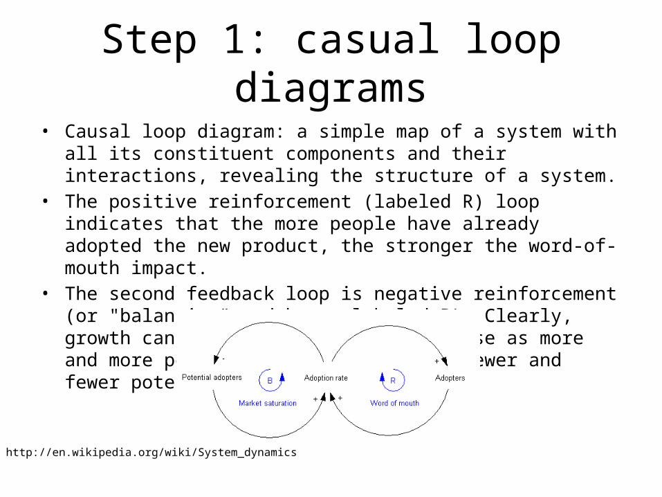
Step 1: casual loop diagrams• Causal loop diagram: a simple map of a system with all its constituent
components and their interactions, revealing the structure of a system. • The positive reinforcement (labeled R) loop indicates that the more
people have already adopted the new product, the stronger the word-of-mouth impact.
• The second feedback loop is negative reinforcement (or "balancing" and hence labeled B). Clearly, growth cannot continue forever, because as more and more people adopt, there remain fewer and fewer potential adopters.
http://en.wikipedia.org/wiki/System_dynamics

Step 1: dynamic casual loop diagrams• Both feedback loops act simultaneously, but at different times they may
have different strengths. Thus one would expect growing sales in the initial years, and then declining sales in the later years.
-step1 : (+) green arrows show that Adoption rate is function of Potential Adopters and Adopters
-step2 : (-) red arrow shows that Potential adopters decreases by Adoption rate
-step3 : (+) blue arrow shows that Adopters increases by Adoption rate

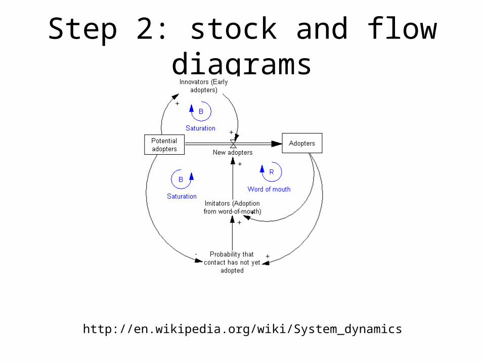
Step 2: stock and flow diagrams
• The next step is to create what is termed a stock and flow diagram. A stock is the term for any entity that accumulates or depletes over time. A flow is the rate of change in a stock.
• In this example, there are two stocks: Potential adopters and Adopters. There is one flow: New adopters. For every new adopter, the stock of potential adopters declines by one, and the stock of adopters increases by one.
http://en.wikipedia.org/wiki/System_dynamics
Step 2: stock and flow diagrams
http://en.wikipedia.org/wiki/System_dynamics

Step 3: write equations
http://en.wikipedia.org/wiki/System_dynamics

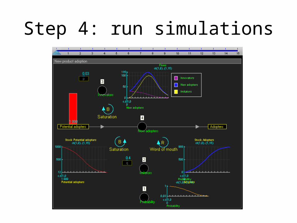
Step 4: run simulations
• Estimate the parameters and initial conditions. These can be estimated using statistical methods, expert opinion, market research data or other relevant sources of information.
• Simulate the model and analyze results
http://en.wikipedia.org/wiki/System_dynamics

Example of piston motion
• Objective : study of a crank-connecting rod system. Model a crank-connecting rod system through a system dynamic model. The crank, with variable radius and angular frequency, will drive a piston with a variable connecting rod length.
• System dynamic modeling:

Example of piston motion
• Simulation : the behavior of the crank-connecting rod dynamic system can then be simulated.

Example: mathematical epidemiologySusceptibles Infectives Removals (SIR) model
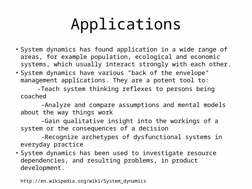
Applications• System dynamics has found application in a wide range of areas, for
example population, ecological and economic systems, which usually interact strongly with each other.
• System dynamics have various "back of the envelope" management applications. They are a potent tool to:
-Teach system thinking reflexes to persons being coached -Analyze and compare assumptions and mental models about the
way things work -Gain qualitative insight into the workings of a system or the
consequences of a decision -Recognize archetypes of dysfunctional systems in everyday
practice • System dynamics has been used to investigate resource
dependencies, and resulting problems, in product development. http://en.wikipedia.org/wiki/System_dynamics

Discussion
• Use the system dynamics model to model the grass sheep ecological system
Discussion
• The space is not modeled. • All grass and sheep are treated in the same
way – no heterogeneity. • It is difficult to add more “behaviors”, such as
sheep’s adaptation to the environment, to the sheep.

An Agent-based Model for Studying Child Maltreatment and Child Maltreatment
Prevention
Xiaolin Hu, PhD, Georgia State University Richard W. Puddy, PhD, MD, Centers for Disease Control and
Prevention (CDC)
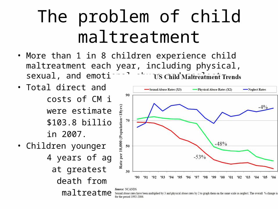
The problem of child maltreatment
• More than 1 in 8 children experience child maltreatment each year, including physical, sexual, and emotional abuse and neglect.
• Total direct and indirect costs of CM in the U.S. were estimated at $103.8 billion annually in 2007. • Children younger than 4 years of age are at greatest risk of death from child maltreatment.

CM and its prevention
• Exposure to child maltreatment increases the risk for things like smoking, substance abuse, obesity, depression and in turn increases the risk of diseases such as cancer, heart disease, stroke and many others.
• Research suggests that progress in preventing the nation's worst health problems – such as obesity and diabetes – can be made by investing in programs that promote raising infants and young children in healthy, safe, stable, and nurturing surroundings.
• Despite the importance of CM prevention, many of the current methodologies employed to prevent maltreatment have not fully advanced the field to the point of making significant impact at the population level.
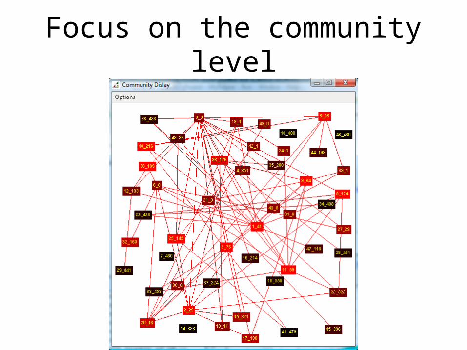
Focus on the community level
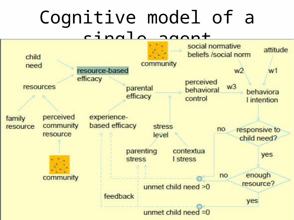
Cognitive model of a single agent

The agent-based model of CM
http://cs.gsu.edu/SIMS/CMSimulation/

Example of CM
• What Will Happen if Reducing Community Stress by 70% after One Year?
Set up a virtual community that is of interest.public double averageChildrenPerHouse = 1.5 public double averageParentsPerHouse = 1.3; public double averageFamilyStressLevel = 4; public double parentalSkill = 60; public double STRESS_COMMUNITY = 8; long seed = 26888083;
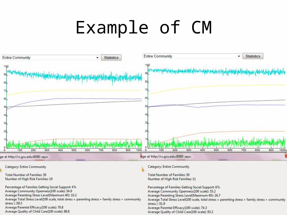
Example of CM

Example of CM• Take A Deeper Look: Different Types of Families in the Community
• Number of Social Connections – Among the 50 Families -10 families have no social connection -17 families have 1 or 2 social connections -23 families have 3 or more social connections
• Family Resource –Among the 50 Families -11 families have 0 or less resources (compared to child need) -12 families have 0-10% more resource (compared to child need) -14 families have 10%-20% more resource (compared to child need) -13 families have >20% more resource (compared to child need)
Note: In each simulation run, the computer program generates an “artificial community” based on users’ configurations. The number of families in each category may be different for different simulation runs.

Example of CM
Based on social connection Based on family resource
Note: In each simulation run, the computer program generates an “artificial community” based on users’ configurations. The number of families in each category may be different for different simulation runs.

Example of CM

Example of CM
• The simulated community has high level of community stress, which make families have high stress levels.
• Based on the model, when families have high stress levels, they tend not to fully exploit their family resources and/or social connections.
• When the community stress is reduced, families with more social connections or more family resources benefit more because they begin to exploit these resources. Families with less resource/social connections “benefit” in a limited way because they have limited resource to exploit.
• Will this pattern be true for a different type of community? • Is this correct in the real world?

A system dynamics model
http://forio.com/simulate/chris.soderquist/ssnr-ll/overview/

Using a Systems Dynamics Framework to Improve State Policy-making Karen J. Minyard, Rachel Ferencik, Chris Soderquist, Heather Devlin, Mary Ann Phillips,
Ken Powell Academy Health
State Health Research and Policy Interest Group June 27, 2009

Dynamics in the Dual Eligible Population: A Systems Map Georgia Health Policy Center Communities Joined in Action

Discussion
• The relationship and the difference between the two models.
-What advantages can the SDM bring? -What advantages can the ABM bring? • How can the two models work together?

Heterogeneity and network structure in the dynamics of diffusion: comparing agent-based
and differential equation models
Hazhir Rahmandad, John Sterman, .Heterogeneity and network structure in the dynamics of diffusion: comparing agent-based and differential equation models., available HTTP: http://www.mit.edu/ hazhir/papers/Rahmandad-Sterman 051222.pdf

DE models and AB models• Each method has strengths and weaknesses. • Nonlinear DE models often have a broad boundary encompassing a
wide range of feedback effects but typically aggregate agents into a relatively small number of states (compartments).
• For example, models of innovation diffusion may aggregate the population into categories including unaware, aware, in the market, recent adopters, and former adopters (Urban, Hauser and Roberts, 1990; Mahajan, Muller and Wind, 2000).
• However, the agents within each compartment are assumed to be homogeneous and well mixed; the transitions among states are modeled as their expected value (possibly perturbed by random events).
• Another common difference is the representation of time. In DE models time is continuous. AB models are typically formulated in discrete time, with agents interacting at intervals.
DE models and AB models
• In contrast, AB models can readily include heterogeneity in agent attributes and in the network structure of their interactions; like DE models, these interactions can be deterministic or stochastic.
• However, the increased detail comes at the cost of introducing large numbers of parameters.
• It can be difficult to analyze the behavior of an AB model, and the computing resources required to carry out sensitivity tests can be prohibitive.
• Understanding where the agent-based approach yields additional insight and where such detail is unimportant is central to selecting appropriate methods for any problem at hand.
• We argue that AB and DE models are more productively viewed as points on a spectrum of aggregation assumptions rather than as fundamentally incompatible modeling paradigms.
Experiment setup• We develop an AB version of the classic SEIR model, a widely used lumped
nonlinear deterministic DE model (see e.g. Murray 2002). • The DE version divides the population into four compartments: Susceptible
(S), Exposed (E), Infected (I), and Recovered (R). • In the AB model, each individual is separately represented and must be in
one of the four states. • To ensure comparability of the AB and DE models, we implement them in the
same software environment and show how a stochastic AB model can be formulated in continuous time so that the same numerical integration procedure can be used in both.
• We set the (mean) values of parameters in the AB model equal to those of the DE. Therefore any differences in outcomes arise only from the relaxation of the mean-field aggregation assumptions of the DE model.
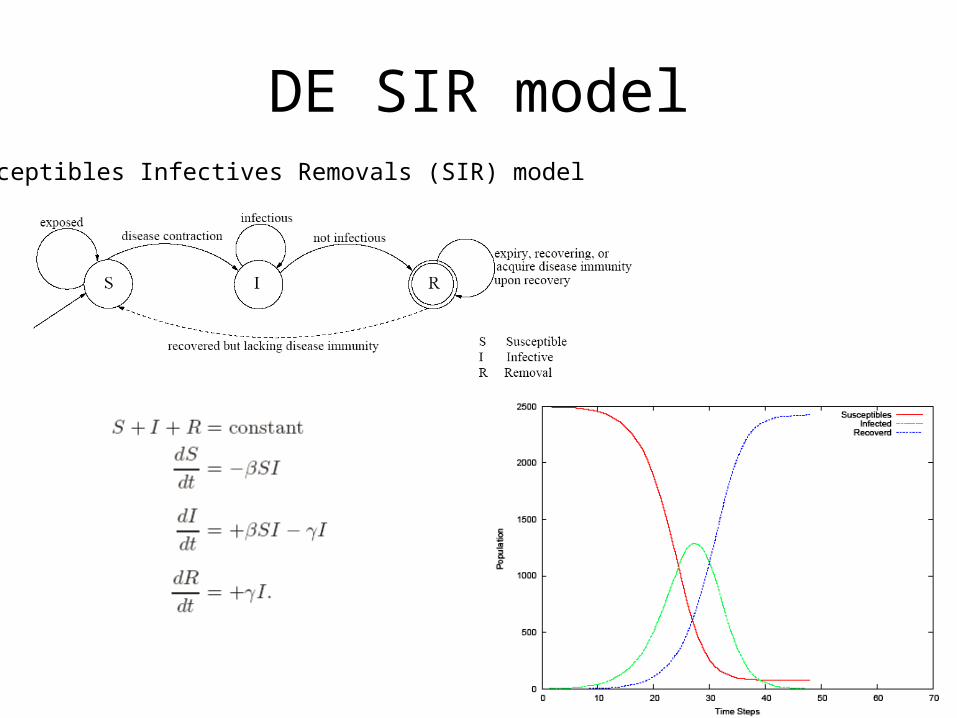
DE SIR modelSusceptibles Infectives Removals (SIR) model

Experiment setup• We run the AB model under five different network structures, including fully
connected, random, Watts-Strogatz small world, scale-free, and lattice. • The fully connected network is closest to the perfect mixing assumption of
the DE; the lattice, with connections solely to neighbors, is most different; the small world and scale free networks are widely used and characterize many real situations (Watts and Strogatz 1998; Barabasi and Albert 1999; Barabasi 2002).
• We test each network structure with homogeneous and heterogeneous agent attributes such as the rate at which each agent contacts others.
• We compare the DE and AB epidemics on a variety of key metrics relevant to public health, including the fraction of the population ultimately infected (the total burden of disease), the maximum prevalence of infectious cases (a measure of the peak load on public health infrastructure), and the time to the peak of the epidemic (indicating how much time health officials have to respond).

Results• Experiment results see paper on P. 29, 30 • Surprisingly, however, the differences between the DE and AB models are
not statistically significant for key metrics such as peak time, peak prevalence, and disease burden in any but the lattice network. Though the small-world and scale-free networks are highly clustered, their dynamics are close to the DE model: even a few long-range contacts and highly connected hubs seed the epidemic at multiple points in the network, enabling it to spread rapidly.
• We also examine the ability of the DE model to capture the dynamics of each network structure in the realistic situation where data on underlying parameters are not available. Surprisingly, the fitted DE model matches the mean behavior of the AB model under all network structures and heterogeneity conditions tested.
Results• The parsimony and robustness of the DE model suggests these models remain useful
and appropriate in many situations, particularly where network structure is unknown or labile and where fast turnaround is required.
• The detail and flexibility of the AB models are likely to be most helpful where the structure of the contact network is known, stable, and highly localized, and where it is important to understand the impact of stochastic events on the range of likely outcomes.
• Further, since time and resources are always limited, modelers must trade off the data requirements and computational burden of disaggregation against the breadth of the model boundary.
• AB models will be most appropriate where results depend delicately on agent heterogeneity and random events. DE models will be most appropriate where results hinge on the incorporation of a wide range of feedbacks with other system elements (a broad model boundary).
• We suggest the complementary strengths and weaknesses of each model type can be used to advantage when DE and AB elements are integrated in a single model.

System Dynamics Modeler of NetLogo
• Program how populations of agents behave as a whole, For example, using System Dynamics to model Wolf-Sheep Predation, you specify how the total number of sheep would change as the total number of wolves goes up or down, and vice versa. You then run the simulation to see how both populations change over time.
• The System Dynamics Modeler allows you to draw a diagram that defines these populations, or "stocks", and how they affect each other.
• The Modeler reads your diagram and generates the appropriate NetLogo code -- global variables, procedures and reporters -- to run your System Dynamics model inside of NetLogo.

System Dynamics Modeler of NetLogo
• A System Dynamics diagram has four kinds of elements - Stocks -Variables -Flows -Links• Stock, a collection of stuff, an aggregate, e.g., a stock can represent a
population of sheep, the water in a lake, or the number of widgets in a factory.
• Flow, brings things into, or out of a Stock. Flows look like pipes with a faucet because the faucet controls how much stuff passes through the pipe.
• Variable, a value used in the diagram, can be an equation that depends on other Variables, or it can be a constant.
• Link, makes a value from one part of the diagram available to another. A link transmits a number from a Variable or a Stock into a Stock or a Flow.
System Dynamics Modeler of NetLogo
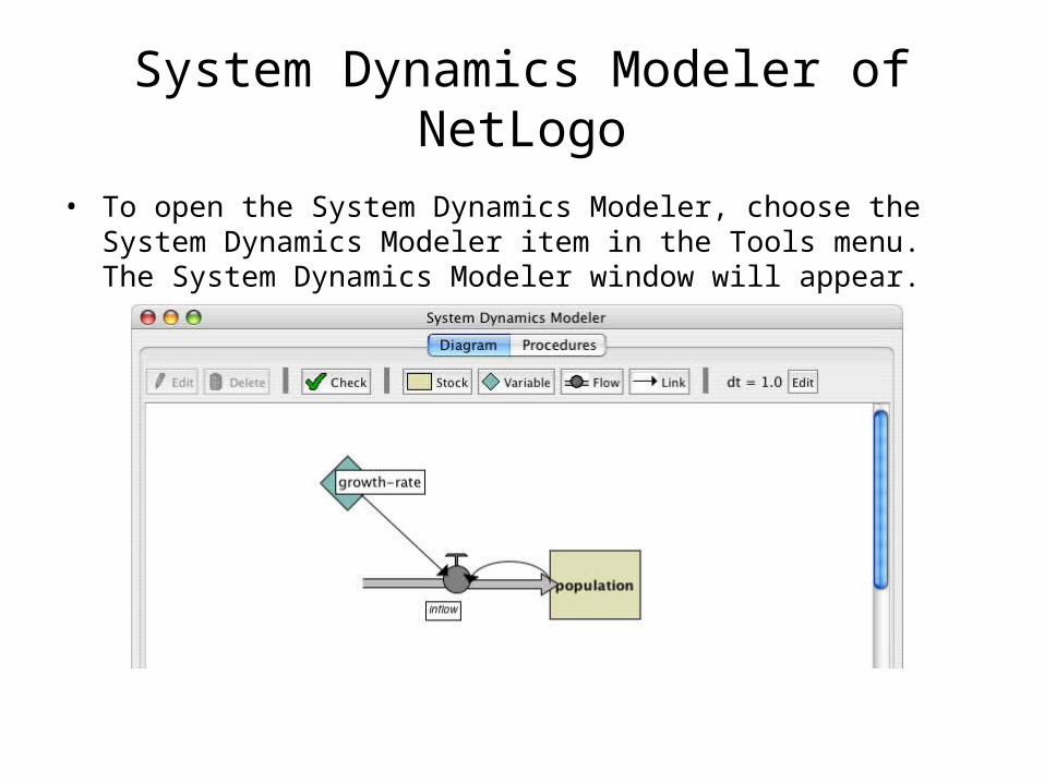
• To open the System Dynamics Modeler, choose the System Dynamics Modeler item in the Tools menu. The System Dynamics Modeler window will appear.

System Dynamics Modeler of NetLogo
• The toolbar contains buttons to edit, delete, and create items in your diagram• Creating diagram elements
• Stock, press the Stock button in the toolbar and click in the diagram area below. Each Stock needs a unique name, an initial value (a number, variable, a complex NetLogo expression, or a call to NetLogo reporter).
• Variable, press the Variable button and click on the diagram. It requires a unique name (a procedure or a global variable) and an Expression (a number, a variable, a NetLogo expression, or reporter).
• Flow, press the Flow button. Click and hold where you want the Flow to begin – either on a Stock or in an empty area—and drag the mouse to where you want the Flow to end – on a Stock or an empty area. It needs a unique name (reporter) and an Expression (the rate of flow from the input to output, can be any of the four types above).
• Link, click and hold on the starting point for the link -- a Variable, Stock or Flow-- and drag the mouse to the destination Variable or Flow.

System Dynamics Modeler of NetLogo
• Working with Diagram Elements -When create a Stock, Variable, or Flow, a red question-mark on the element. It
indicates that the element doesn't have a name yet. The red color indicates that the Stock is incomplete: it's missing one or more values required to generate a System Dynamics model. When a diagram element is complete, the name turns black.
• Selecting: To select a diagram element, click on it. To select multiple elements, hold the shift key. You can also select one or more elements by dragging a selection box.
• Editing: To edit a diagram element, select the element and press the "Edit" button on the toolbar. Or just double-click the element. (You can edit Stocks, Flows and Variables, but you can't edit Links).
• Moving: To move a diagram element, select it and drag the mouse to a new location.
• Editing dt -On the right side of the toolbar is the default dt, the interval used to approximate
the results of your System Dynamics model. To change the value of the default dt for your aggregate model, press the Edit button next to the dt display and enter a new value.
System Dynamics Modeler of NetLogo
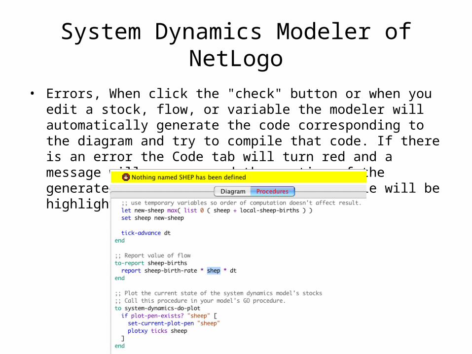
• Errors, When click the "check" button or when you edit a stock, flow, or variable the modeler will automatically generate the code corresponding to the diagram and try to compile that code. If there is an error the Code tab will turn red and a message will appear, and the portion of the generated code that is causing the trouble will be highlighted.

System Dynamics Modeler of NetLogo
• Code Tab, displays the NetLogo procedures generated from your diagram. You can't edit the contents of the Code tab. To modify System Dynamics mode, edit the diagram.
• Stocks correspond to a global variable that is initialized to the value or expression you provided in the Initial value field. Each Stock will be updated every step based on the Flows in and out.
• Flows correspond to a procedure that contains the expression you provided in the Expression field.
• Variables can either be global variables or procedures. If the Expression you provided is a constant it will be a global variable and initialized to that value. If you used a more complicated Expression to define the Variable it will create a procedure like a Flow.
System Dynamics Modeler of NetLogo
• The variables and procedures defined in this tab are accessible in the main NetLogo window, just like the variables and procedures you define yourself in the main NetLogo Code tab. You can call the procedures from the main Code tab, from the Command Center, or from buttons in the Interface tab. You can refer to the global variables anywhere, including in the main Code tab and in monitors.
• Three important procedures to notice: system-dynamics-setup, system-dynamics-go, and system-dynamics-do-plot.
• system-dynamics-setup initializes the aggregate model. It sets the value of dt, calls reset-ticks, and initializes your stocks and your converters. Converters with a constant value are initialized first, followed by the stocks with constant values. The remaining stocks are initialized in alphabetical order.
• system-dynamics-go runs the aggregate model for dt time units. It computes the values of Flows and Variables and updates the value of Stocks. It also calls tick-advance with the value of dt. Converters and Flows with non-constant Expressions will be calculated only once when this procedure is called, however, their order of evaluation is undefined.

System Dynamics Modeler of NetLogo
• system-dynamics-do-plot plots the values of Stocks in the aggregate model. To use this, first create a plot in the main NetLogo window. You then need to define a plot pen for each Stock you want to be plotted. This procedure will use the current plot, which you can change using the set-current-plot command.
• The diagram you create with the System Dynamics Modeler, and the procedures generated from your diagram, are part of your NetLogo model. When you a save the NetLogo model, your diagram is saved with it, in the same file.

Tutorial• Open a new model in NetLogo.• Launch the System Dynamics Modeler in the Tools menu.
• Press the Stock button in the toolbar.
• Click in the diagram area.

Tutorial• Double-click the Stock to edit.• Name the stock sheep• Set the initial value to 100.• Deselect the Allow Negative Values checkbox. It doesn't make sense to
have negative sheep!

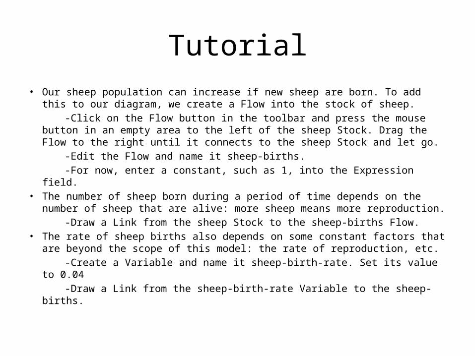
Tutorial• Our sheep population can increase if new sheep are born. To add this to
our diagram, we create a Flow into the stock of sheep. -Click on the Flow button in the toolbar and press the mouse button in an
empty area to the left of the sheep Stock. Drag the Flow to the right until it connects to the sheep Stock and let go.
-Edit the Flow and name it sheep-births. -For now, enter a constant, such as 1, into the Expression field.• The number of sheep born during a period of time depends on the
number of sheep that are alive: more sheep means more reproduction. -Draw a Link from the sheep Stock to the sheep-births Flow.• The rate of sheep births also depends on some constant factors that are
beyond the scope of this model: the rate of reproduction, etc. -Create a Variable and name it sheep-birth-rate. Set its value to 0.04 -Draw a Link from the sheep-birth-rate Variable to the sheep-births.

Tutorial• The diagram looks like the following.
• The sheep-births Flow has a red label because we haven't given it an expression. Red indicates that there's something missing from that part of the diagram.
• The amount of sheep flowing into our stock will depend positively with the number of sheep and the sheep birth rate.
-Edit the sheep-births Flow and set the expression to sheep-birth-rate *sheep.

Tutorial
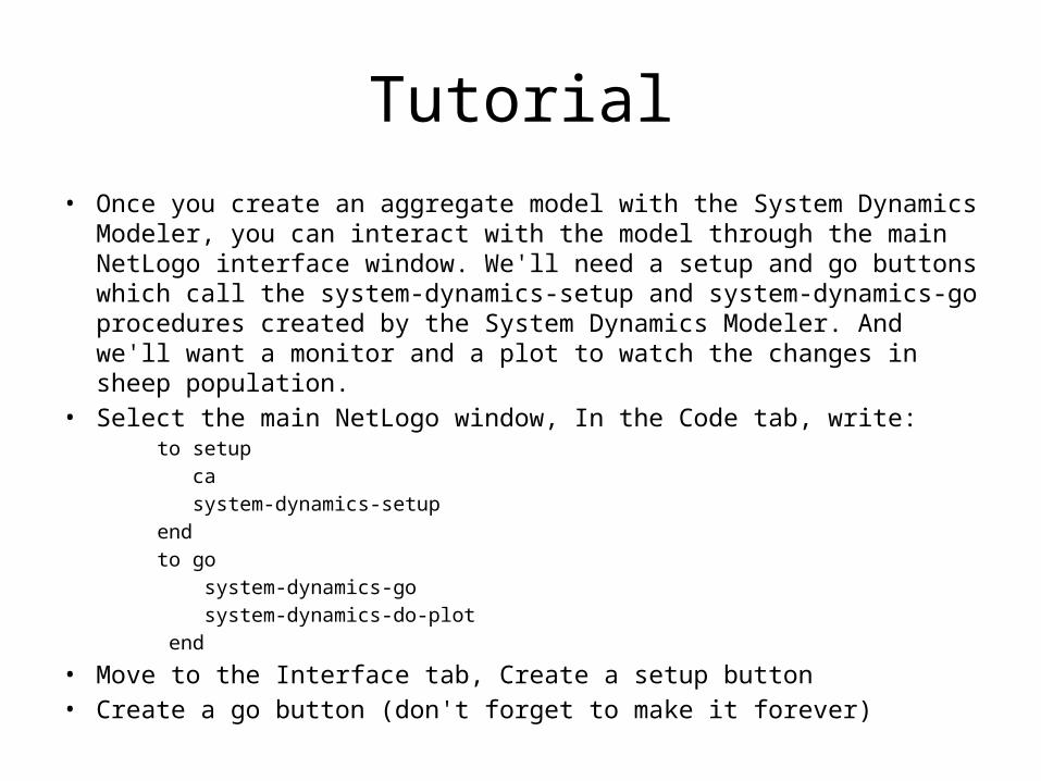
Tutorial• Once you create an aggregate model with the System Dynamics Modeler, you
can interact with the model through the main NetLogo interface window. We'll need a setup and go buttons which call the system-dynamics-setup and system-dynamics-go procedures created by the System Dynamics Modeler. And we'll want a monitor and a plot to watch the changes in sheep population.
• Select the main NetLogo window, In the Code tab, write: to setup ca system-dynamics-setup end to go system-dynamics-go system-dynamics-do-plot end
• Move to the Interface tab, Create a setup button• Create a go button (don't forget to make it forever)
Tutorial• Create a sheep monitor.• Create a plot called "populations" with a pen named "sheep".• The sheep population increases exponentially. After four or five iterations,
we have an enormous number of sheep. That's because we have sheep reproduction, but our sheep never die.
• To fix that, let's finish our diagram by introducing a population of wolves which eat sheep.
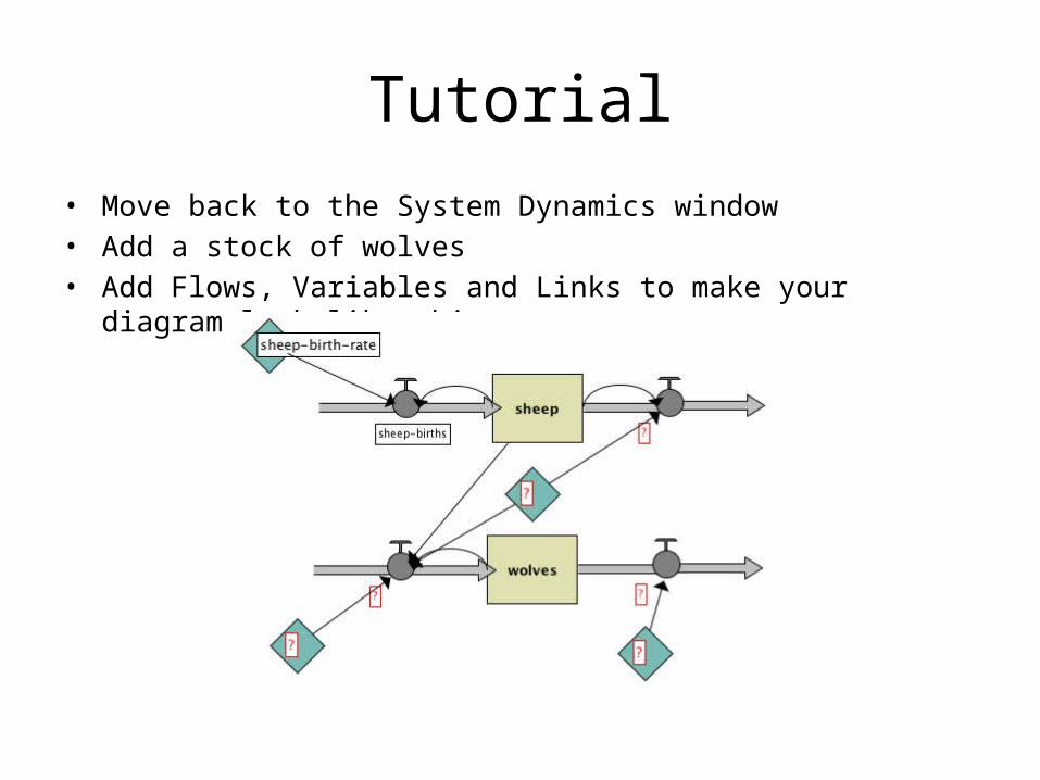
Tutorial• Move back to the System Dynamics window• Add a stock of wolves• Add Flows, Variables and Links to make your diagram look like this:

Tutorial• Add one more Flow from the wolves Stock to the Flow that goes out of the
Sheep stock.• Fill in the names of the diagram elements so it looks like this:
whereinitial-value of wolves is 30,wolf-deaths is wolves * wolf-death-rate ,wolf-death-rate is 0.15,predator-efficiency is .8,wolf-births is wolves * predator-efficiency * predation-rate * sheep,predation-rate is 3.0E-4,and sheep-deaths is sheep * predation-rate * wolves.

Tutorial• Go to the main window, add a plot pen "wolves" to the population plot,
press setup and see your System Dynamics Modeler diagram in action.